1. Introduction
The consumption of energy by industrial and domestic electric motors per year occupies 46.2% of the global electrical demand [
1]. In addition, electrical vehicles (EVs) have continuously attracted the attention of researchers and companies [
2,
3]. Due to its high power density, efficiency, low maintenance cost, and wide range speed regulation, an interior permanent magnet synchronous motor (IPMSM) is an attractive selection for EVs and hybrid electric vehicles (HEVs) [
4]. In order to achieve high compactness and to abstain from a multi-stage gearbox, an electrical traction drive usually has a wide constant power speed range (up to 12,000 rpm) [
5] to cover the high driving speed of the EVs.
Traditionally, the d-axis stator current component of the IPMSM is set at zero in the current/torque control for easier design. However, the efficiency of the drive system cannot be optimized without controlling the air gap flux. As a result, the reluctance torque of the IPMSM, which is one of its advantages as compared with a surface-mounted PMSM, cannot be utilized. In order to improve this and extend the speed range, it is necessary to maximize the IPMSM torque output appropriately along the optimal current trajectory over the whole speed range. The typical IPMSM current trajectory on the
plane may consist of three or four paths or regions [
6,
7,
8], as shown in
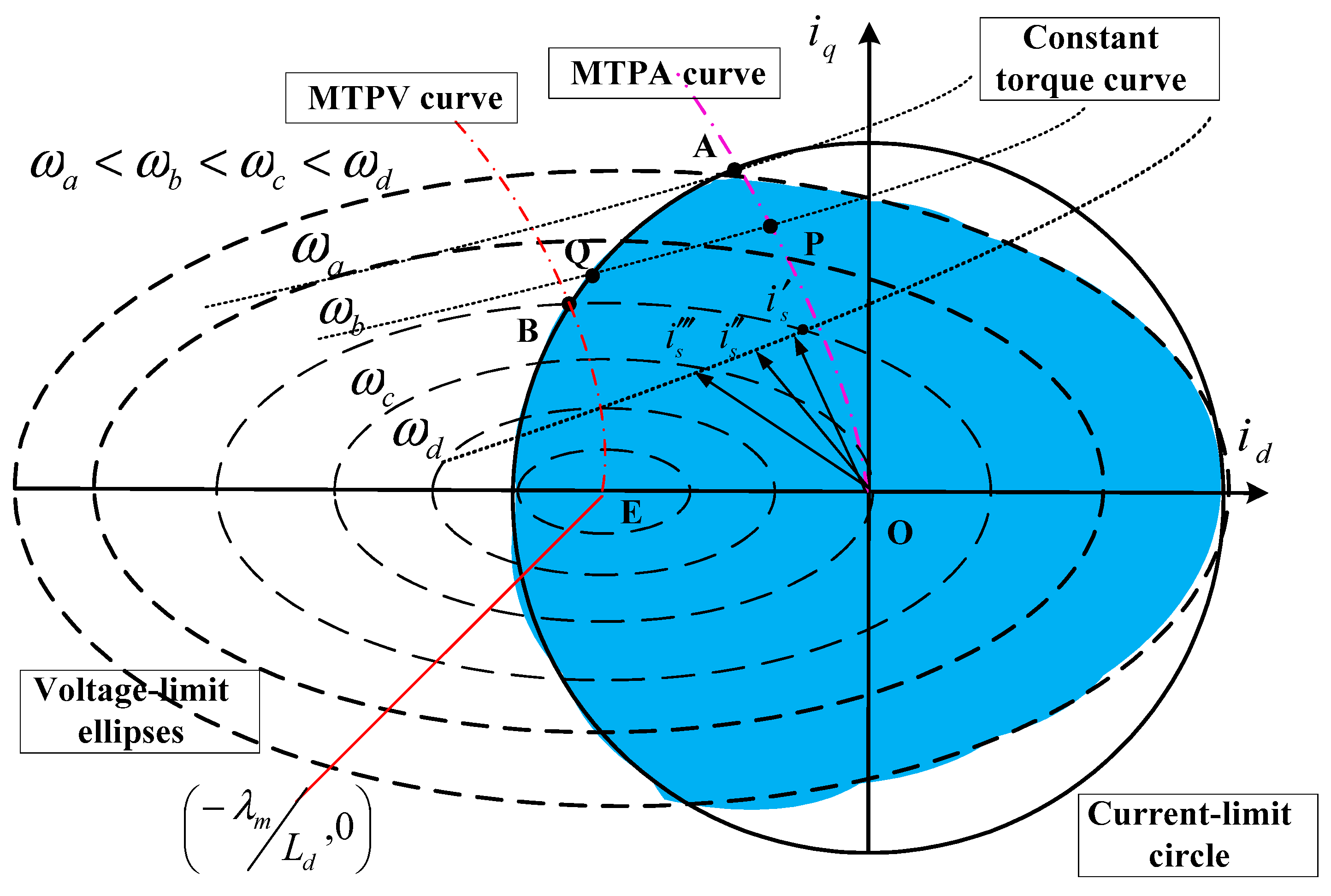
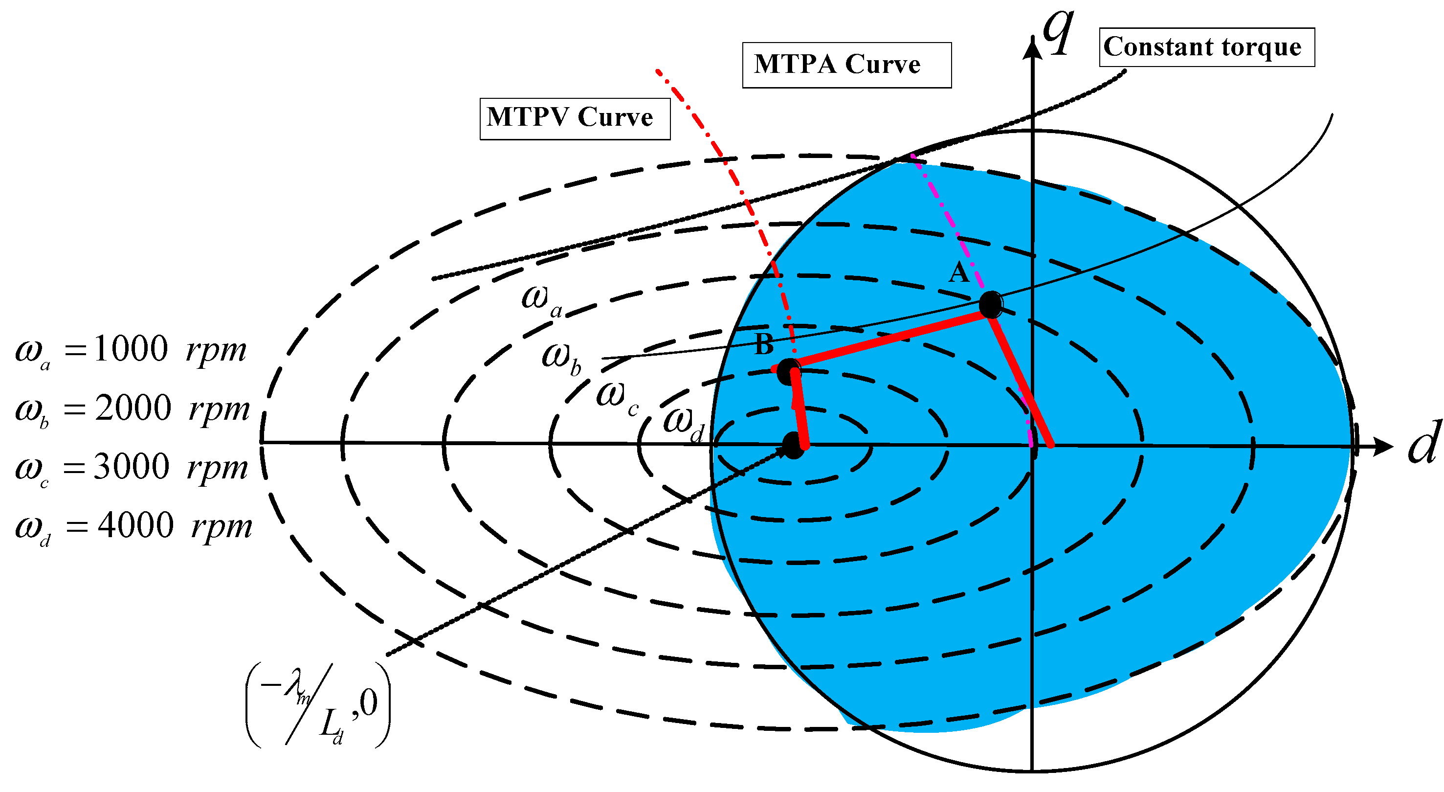
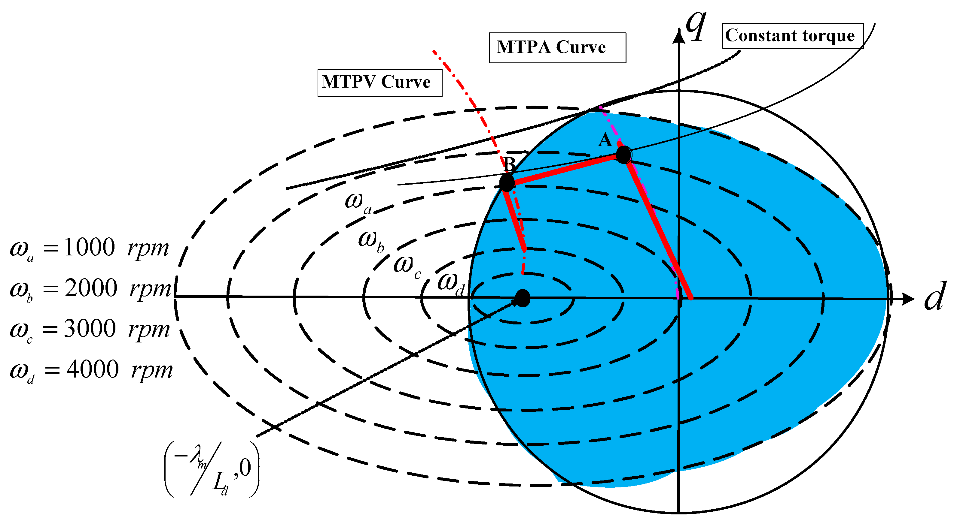
Figure 1. Region 1 (curve OP) is the maximum torque per ampere (MTPA) operation that generates the required torque with a minimum phase current. Region 2 (hyperbola PQ) moves the current trajectory away from the MTPA curve along the torque hyperbola. Optional Region 3 (arc QB) starts the flux-weakening operation and moves the current trajectory along the current limitation circle. Region 4 (curve BE) is the maximum torque per voltage (MTPV) operation to generate possible maximum torque under the inverter voltage limitation.
The MTPA control means that the ratio between the produced torque and the current amplitude is maximized through properly selecting the current space vector as a torque function. The MTPV control is used to increase the motor speed further and extend the torque control capability under the voltage-limited maximum output current vector control if the center of the voltage-limit ellipses of the motor lies inside the current-limit circle. Generally, this is easy by using the optimum current space vector to understand and conduct the mathematical and graphical analyses of the constant-torque and constant-current loci. However, it requires precise values of motor parameters, such as direct- and quadrature-axis inductances and the flux linkages, and the stator resistance. Essentially, those are not easy to be found over a wide speed range just by considering an optimization problem that considers torque error minimization as the objective function with the inverter voltage and current as constraints. Furthermore, it is usually time-consuming and difficult to directly solve this problem from the closed-form solutions of nonlinear torque, voltage, and current equations.
The recursive least square (RLS) estimation is proposed in Reference [
5] to identify the variable parameters of motor characteristics online for a high speed and high performance IPMSM. It leads to an improvement of the efficiency by around 6% from 79% using the method with constant parameters. A model linearization-based approach is proposed in Reference [
6]. The optimal torque control problem over a wide speed range is divided into two sub-optimizations to solve them sequentially to simplify the calculation. However, only simulation results were provided. Linear field-weakening control (LFC) of IPMSM is proposed in Reference [
7] to prevent losing current control due to the saturation of current regulators for nonlinear field-weakening in wide speed range applications. As a result, the operation range is only divided into three areas, that is, constant torque linear area, constant power transition linear area, and constant direct axis current area. However, due to the uncertainties of the characteristics of the voltage source, inductance, and the permanent magnet flux linkage, the torque and power performance needs to be improved. Direct torque and flux control (DTFC) is used to especially investigate the deep flux-weakening control of an IPMSM along the maximum torque per voltage (MTPV) trajectory in the torque-flux plane [
8,
9]. A feedforward look-up-table-based method is proposed [
10] to consider the motor parameter variation as the motor operates along the MTPV region by controlling both the voltage and current vectors. In addition to a look-up table, this method was relatively complicated [
11].
It is well known that intelligent control has the advantages of being without need of an exact system dynamic model, simplicity, less intensive mathematical design, and is suitable for dealing with the nonlinearities and uncertainties. Fuzzy logic control (FLC), neural network control (NNC), and neurofuzzy control (NFC), etc., belong to intelligent control. In addition, FLC is the simplest one for implementation. Therefore, a fuzzy logic controller is applied in many fields [
12,
13,
14,
15,
16,
17,
18,
19]. Contrary to the conventional FLC of a IPMSM drive with zero d-axis current, a simplified fuzzy speed controller with MTPA incorporated for the IPMSM drive is proposed [
20]. It simplified the d-axis current around some operating point to get the electromagnetic torque. The authors in Reference [
21] proposed the FLC based IPMSM drive with variable d-axis and q-axis current equations to investigate the performance and compare it to that obtained from the drive via calculating dynamic MTPA equations using MATLAB/Simulink. An online loss-minimization MTPA algorithm is further integrated with a FLC-based IPMSM drive to yield high efficiency and high dynamic performance over a wide speed range [
22]. A fuzzy control algorithm based on the operation time of zero space voltage vectors [
23] to derive d-axis current for the field-weakening control of PMSM is proposed. The FLC, which outputs d- and q-axis currents of IPMSM, is proposed based on conventional MTPA operation using simplified equation [
24] and the field-weakening operation while maintaining current and voltage constraints. The simulation results of fuzzy MTPA and MTPV control of IPMSM using MATLAB/Simulink is shown to verify the proposed algorithm [
13]. Based on the following reasons, a simple intelligent control algorithm, less computation time, easy implementation by microcontroller/digital signal processor, many successful examples, and MTPA, field weakening, and MTPV all designed over the full speed span in this paper, FLC was adopted.
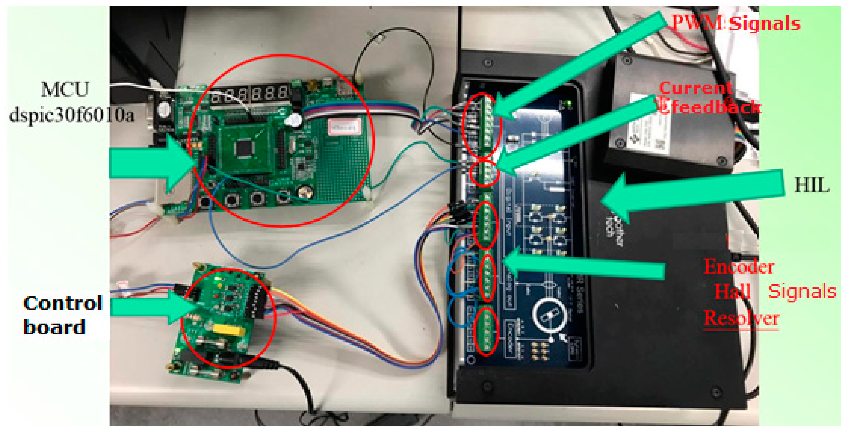
It usually takes a long time and costs much to complete a new designed IPMSM and to verify its performance. A hardware-in-the-loop (HIL) system will be a workable substitute. The MR2 is one HIL system [
25]. It is a virtual reality integration platform designed for controller development, verification, and testing. It enables research and development personnel to conduct product development, verification, and debugging in a safe and convenient real-time simulation environment. Connecting the controller’s I/O terminals, MR2 can quickly receive the signals from and return the operating results in a very short period time to the controller. Users may choose motors according to their needs. Five kinds of system parameters are included: input voltage and feedback signal scaling setup, grid and rectifier module setup, motor parameters setup, velocity sensor module and load torque setup, and customized analog output signals setup.
In this paper, the IPMSM model and the concept of MTPA and MTPV are introduced in
Section 2. In
Section 3, the fuzzy logic control system (FLC) is described. Simulations using MATLAB/Simulink (The MathWorks Inc., 1 Apple Hill Drive Natick, MA, USA) and experiments using the HIL system of the proposed IPMSM drive are shown in
Section 4. Finally, conclusions are given in
Section 5.
2. Modeling IPMSM, MTPA, and MTPV
The voltage equations of the IPMSM in the dq-frame are expressed using Equations (1)–(4) [
4,
5,
6,
7],
where
and
,
and
,
and
, and
and
denote the d- and q-axis voltages, currents, flux linkages, and inductances, respectively;
is the phase resistance;
p is the differential operator;
is the electric speed; and
is the magnet flux linkage. Combining Equations (1) to (4), we obtain:
The electromagnetic torque is then expressed using Equation (7):
where
P is the number of poles,
stands for the magnetic torque, and
is the reluctance torque.
In the real case, the current and voltage are subject to real constraints:
where
is the rated current of the motor and
is the maximum voltage dependent on the dc-link bus and pulse-width modulation (PWM) method. A bold circle and its interior in
Figure 1 depict Equation (8). For simplicity of analysis, at a steady state of the motor running, the voltage drop on resistance was neglected from Equations (5) and (6):
Substituting Equations (10) and (11) into Equation (9) and rearranging it, we obtain ellipses and their interiors with different speeds as shown in
Figure 1 given by Equation (12):
where
is the center;
and
are the lengths of the semi major and the semi minor axes, respectively, for the dashed ellipses; and electric speeds of
. The overlapped area of the circle and ellipses denotes the operable region of the motor drive system. It is easy to find that the lengths of the semi major and the semi minor axes, as well as the overlapped area, will shrink as the motor speed increases. At the same time, the loci of available current vectors are progressively reduced. This is due to the increase of the back electromotive force (EMF) amplitude. That is to say, the voltage limit plays an increasingly dominant role at higher speed operation. The point of tangency using the circle and the ellipse denotes the speed at no load under a maximum operable voltage, where the motor does not output torque. The operable region of the motor system includes four quadrants. The motor mode occupies the first and second quadrants and the generator mode operates in the third and fourth quadrants.
The main purpose of motor torque at low speed is to accelerate the drive system. As the d-axis current is held at zero, the voltage limit ellipse will force the q-axis current to decrease rapidly when the motor speed approaches and exceeds the rated speed. As a result, a fast torque drop occurs. Controlling the phase between the back EMF and the current vector will result in the effect of flux weakening, that is, a negative d-axis current is designed. Under the current constraint of Equation (10), many stator currents can be set to satisfy some specified torque requirement. For example, various stator current vectors—
,
, and
in
Figure 1—provide the same torque under different motor speeds. As a result, the torque–speed envelope is considerably expanded as compared with the case of a zero d-axis current. Furthermore, it will benefit the system by using the optimal torque control to reduce power dissipation or raise efficiency via supplying the same torque using less current.
The relationship between the d- and q-axis stator currents is shown in
Figure 2 with equations as follows:
A new torque equation is generated by substituting Equation (13) into Equation (7):
The maximum torque per ampere (MTPA) is obtained by differentiating Equation (14) with respect to
and setting it to be zero. The angle for the maximum torque output is:
and the d-axis current for MTPA is:
Using Equation (16), the curve of the MTPA shown in
Figure 1 is found in the field weakening region based on various loads. The intersections of the MTPA curve, current circle, and voltage ellipses denote the maximum output torque of the motor running at different speeds. Point A in
Figure 1 depicts the rated torque and speed of the motor. The d-axis current at point A will be:
In the MTPA trajectory, the d- and q-axis current components of the current space vector are found from the intersection between the constant-torque hyperbola and the constant-current circle, with the constraint of minimum length of the current space vector (i.e., the constant-current locus is tangent to the constant-torque locus).
For wider operational speed in the constant power region, a technique called the maximum torque per voltage (MTPV) control is considered by controlling the current vector such that the torque per flux linkage becomes maximal. In the flux-weakening range, if the characteristic current
is less than the rated motor current, the torque controllability can be extended by using MTPV control [
9]. The expressions of
and
for MTPV can be given as:
From Equation (11), Equation (9) and the stator flux are given as:
As a result, the new equation from Equation (7) for torque is:
Similarly, if we differentiate Equation (21) with respect to
λd and set it to be zero, that is,
, we obtain the d-axis flux and current using the following equations for MTPV:
In summary, to produce the maximum output power in all speed ranges considering the condition of both the current and the voltage limits, the optimum current vector is chosen as follows.
Region I (
):
and
are constant values given using Equation (13). The current vector is fixed at point A in
Figure 1. In this region,
and
.
Region II (): and are chosen as the intersection of the current-limit circle and the voltage-limit ellipses. The current vector moves from point A to B along the current-limit circle as the motor speed increases. In this region, and .
Region III (): and are given using Equation (18). The current vector moves from point B to the center of the ellipse along the voltage-limit maximum-output trajectory. In this region, and .
3. Fuzzy Logic Control
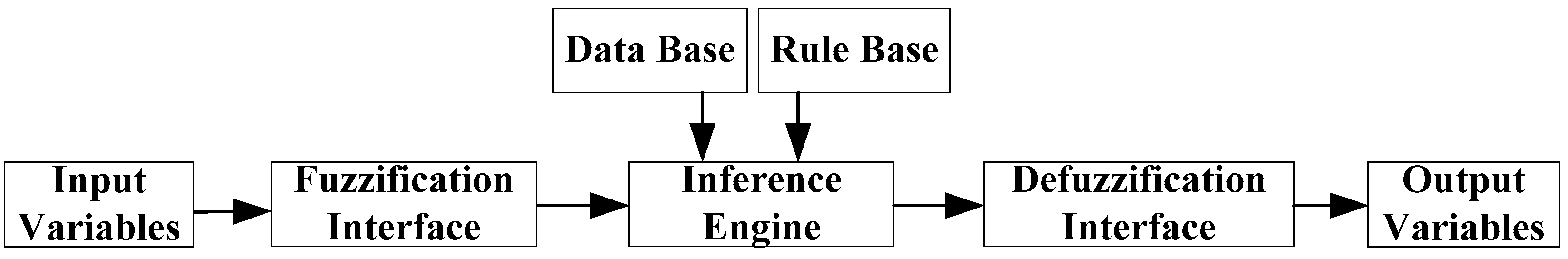
Figure 3 shows the basic blocks of a fuzzy logic control (FLC) system, input variables, the knowledge base (data and rule bases), the inference engine, the fuzzification interface, the defuzzification interface, and output variables. The input and output variables are crisp. The fuzzification interface converts the crisp inputs to fuzzy sets and the defuzzification interface converts these fuzzy conclusions back into the crisp outputs to ensure the desired performance. The fuzzy controller is essentially an artificial and real-time decision-maker in a closed-loop system based on the experts’ experience.
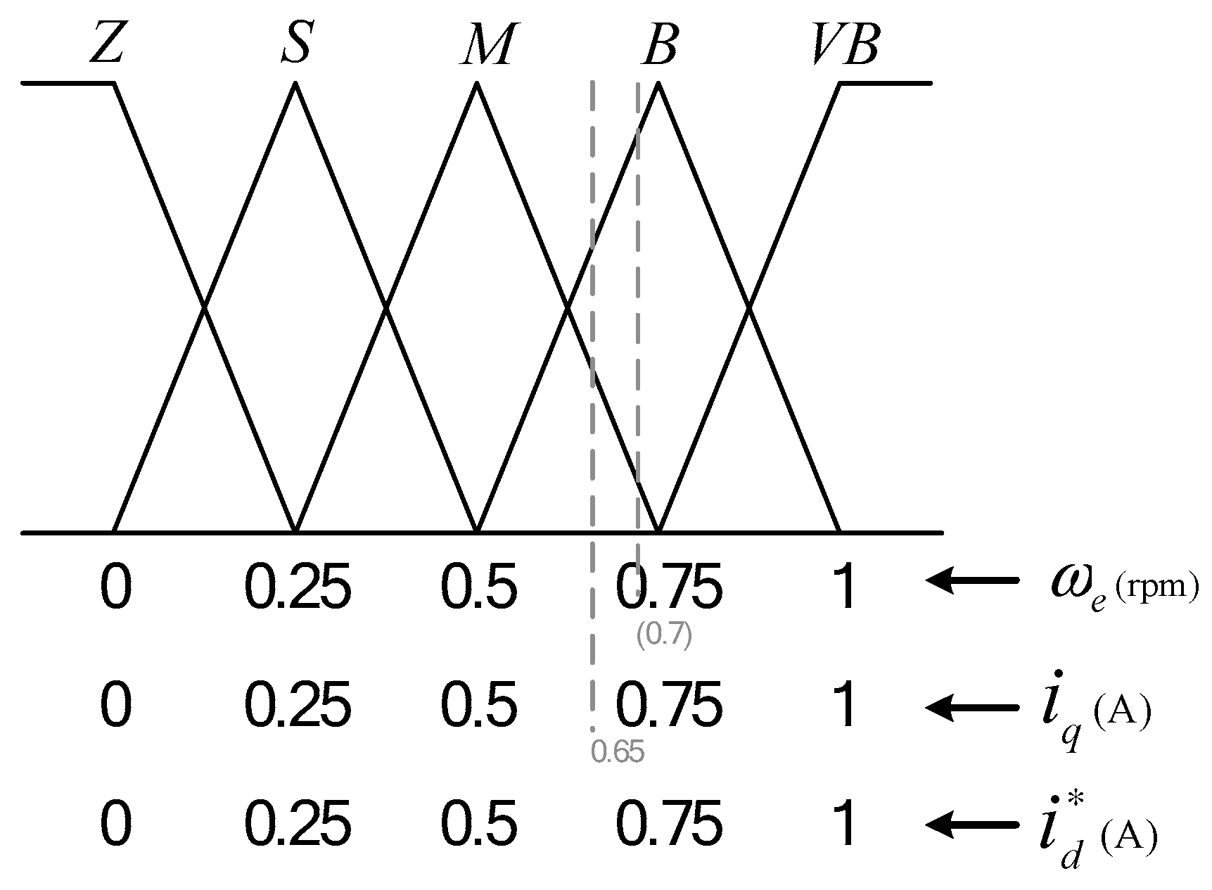
A fuzzy logic control system is used to optimize the MTPA and MTPV as shown in
Figure 4a,b, respectively. The linguistic values Z, S, M, B, and VB represent zero, small, medium, big, and very big, respectively. The membership functions of these input and output fuzzy variables of fuzzy MTPA with normalization are shown in
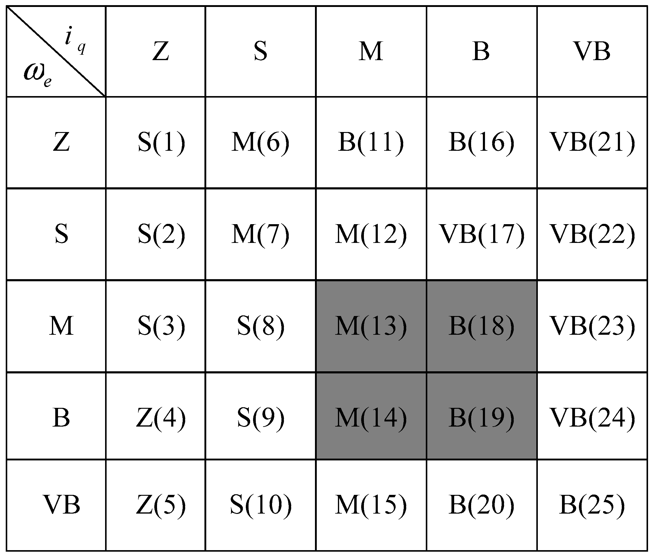
Figure 5, in which the triangular form of the membership functions eases calculating to reduce computation burden of fuzzy MTPA and MTPV. The design methodology does not focus on the specific motor or operation point. It is applicable to any IPMSM. There are 25 rules given in
Figure 6. The first rule is shown as follows.
Rule 1: If is Z and is Z, then is S.
The rule numbers are listed in the parentheses of the table. Rules 13, 14, 18, and 19 are more often triggered. Equation (24) describes the min-min-max inference and mean of height method in the FLC system:
where
is the center of the
ith fuzzy set and
is its height, and
is the center average.
Similarly, the 25 rules for fuzzy MTPV are listed in
Figure 7 since the input variable
iq is only used to check if the magnitude of the stator current vector is larger than the limited value. That is: if
, then
; else, Rule 1: if
is Z and
is Z, then
is S. Rules 8, 9, 13, and 14 are triggered more often.
4. Simulation and Experimental Results
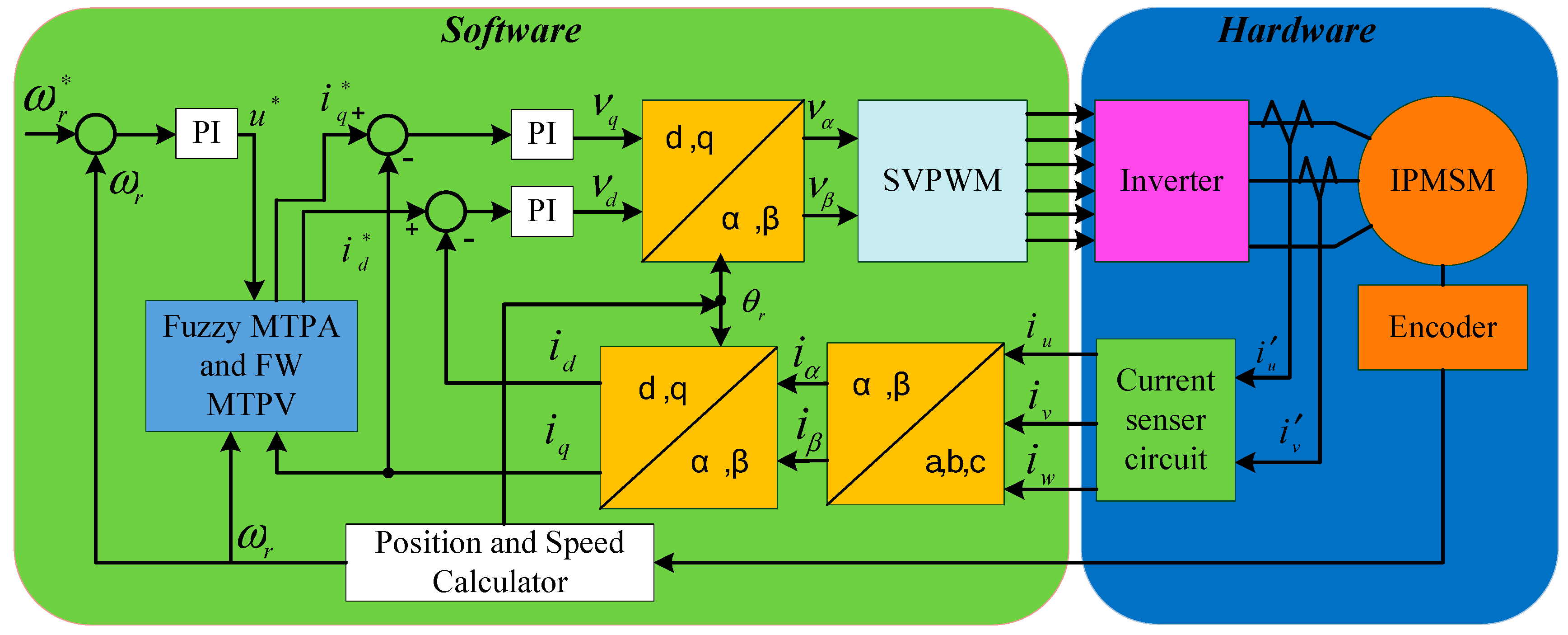
The block diagram of the proposed control system for simulation and experiment, including the test IPMSM, its drive, and servo motor for loading, is shown in
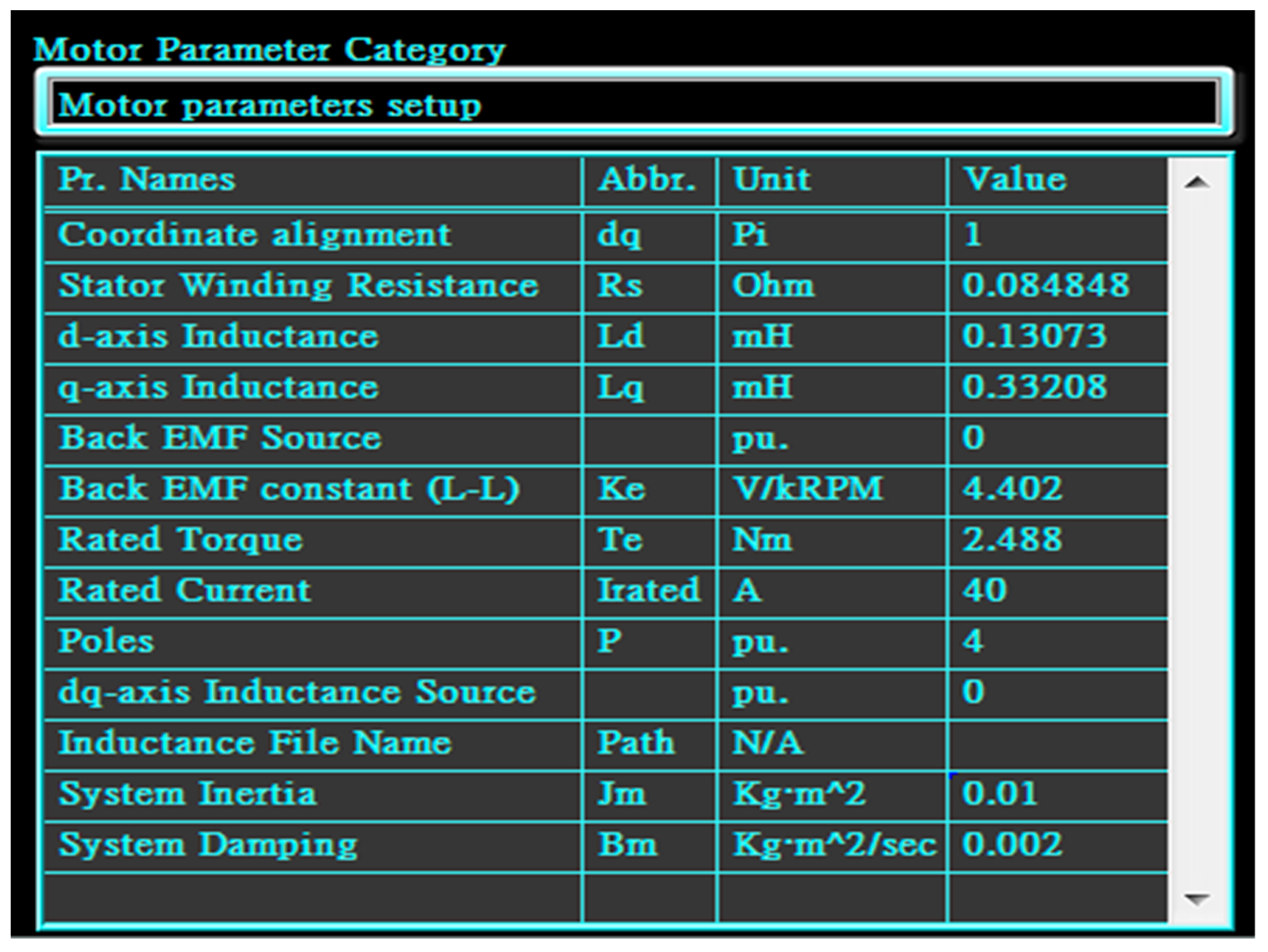
Figure 8. Each block is modeled according to its transfer function. The parameters of IPMSM are listed in
Figure 9 (taken from HIL). There are three proportional and integral (PI) controllers used in the speed and current control loops, respectively. Based on References [
26,
27,
28,
29], the rule of thumb [
30], and our experience, the proportional and integral gains under per-unit processing of speed control loop, d-axis current loop, and q-axis current loop were 0.01 and 0.1, 0.1 and 0.01, and 0.1 and 0.001, respectively. These parameters were adopted and the same in the simulations and experiments.
By using MATLAB/Simulink,
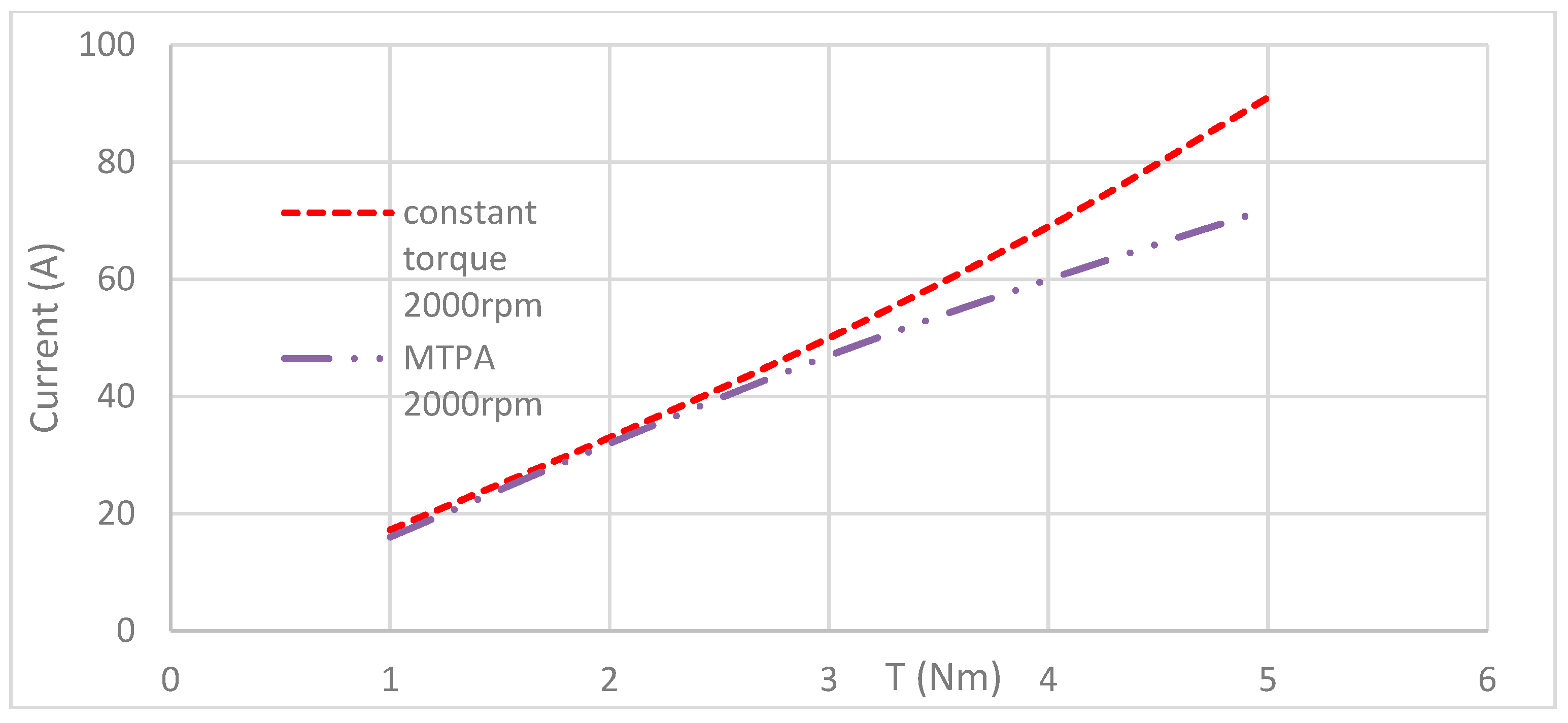
Figure 10 and
Figure 11 show the simulation results of curves of load versus current, respectively, at 300 rpm and 2000 rpm using a fixed torque angle method and fuzzy MTPA control with the loads of 1, 2, 3, 4, and 5 Nm. Under the same load, a lower stator current was needed for fuzzy MTPA control. The difference in stator current for both control methods was larger at a heavy load and for a lower speed range.
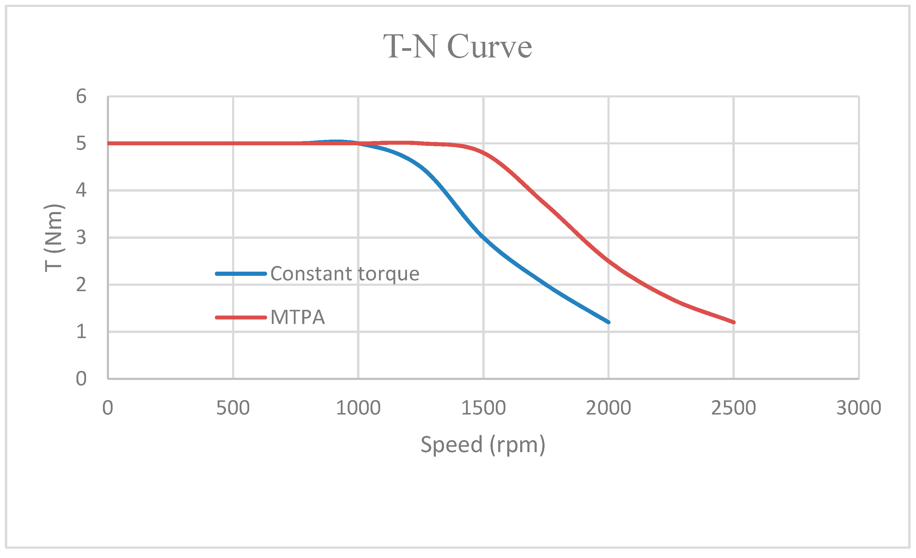
Figure 12 shows the simulation results of the torque–speed curves (called T–N curves hereafter) using a fixed torque angle method and fuzzy MTPA/MTPV control with the load of 5 Nm, double that of the rated torque. The constant torque range shrunk to 1000 rpm, half of the rated speed of 2000 rpm, but the T-N curve using fuzzy MTPA/MTPV control provided a larger torque output and a larger speed range in the constant power region than those using a fixed torque angle method.
MR2 HIL and the related circuits for experiments are shown in
Figure 13.
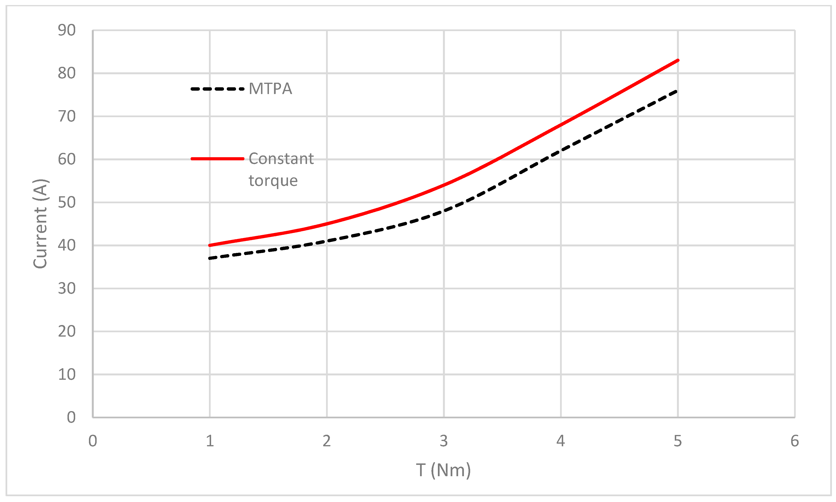
Figure 14 and
Figure 15 show the results of curves of load versus current at 900 rpm and 2000 rpm using a fixed torque angle method and fuzzy MTPA control with the loads of 1, 2, 3, 4, and 5 Nm. The results provided the same conclusions of simulation, but with a larger current at light load, about 20 A. In addition, the differences of stator current for both control was almost independent of motor speed.
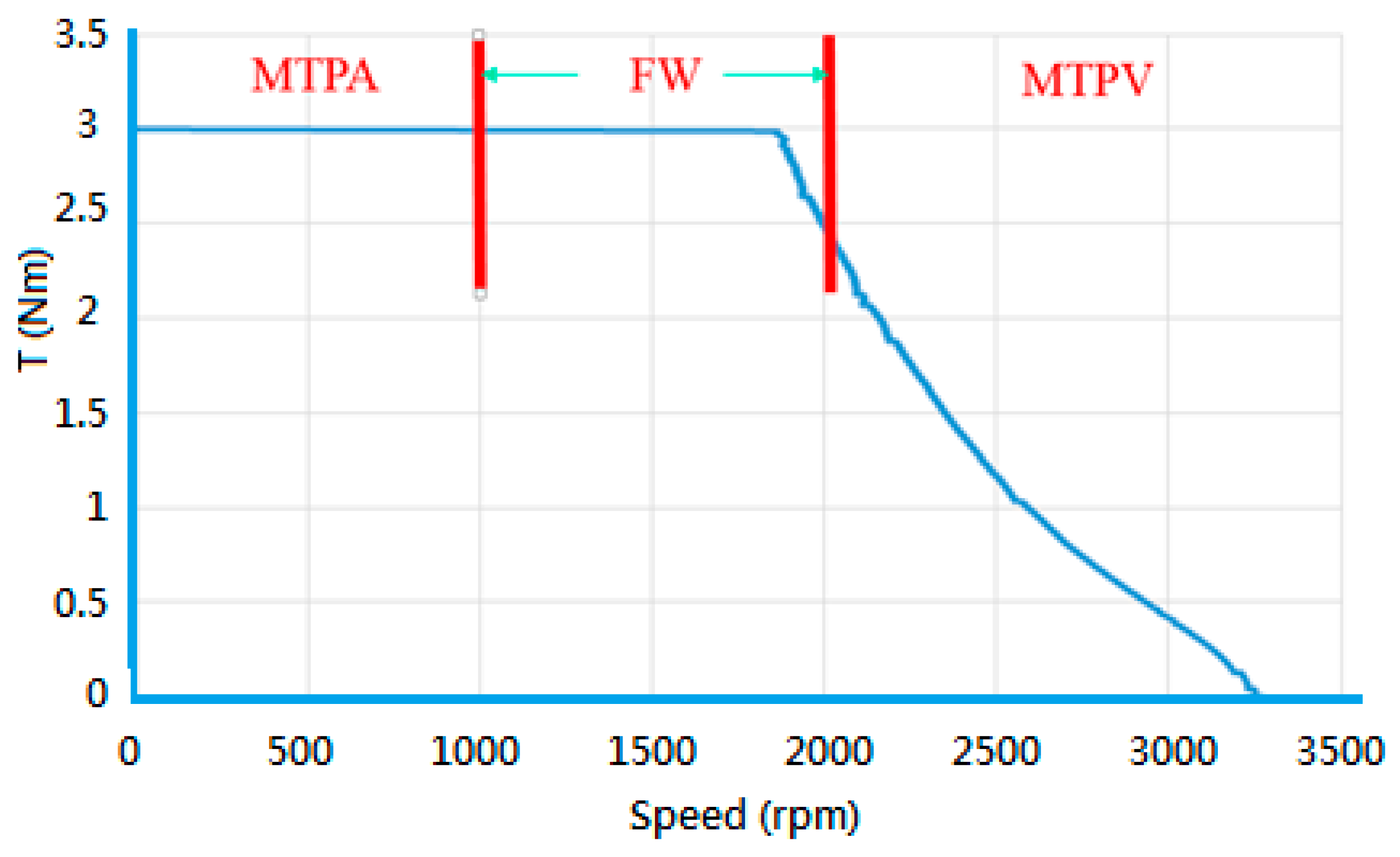
Figure 16 depicts the locus of stator current (bold red) with a load of 3 Nm under the drive current and voltage constraints. The corresponding T–N curve using MTPA, field weakening, and MTPV control in the whole speed range is shown in
Figure 17. It can be found that the constant torque region ended at the speed of 1900 rpm, but it had a larger torque output in the constant power region than that of the rated power. For the situation of rated load, the locus of the stator current (bold red) is drawn in
Figure 18.
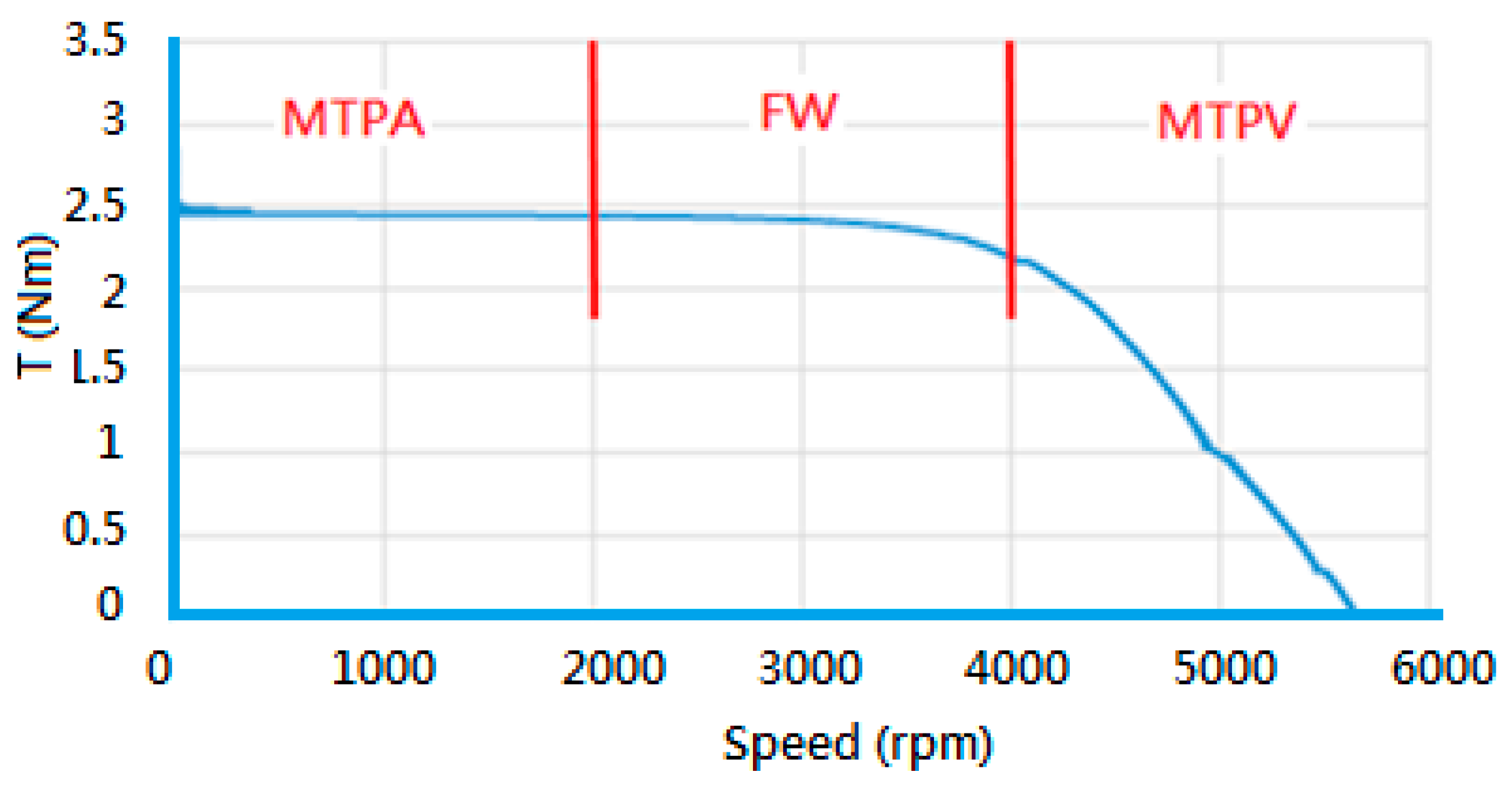
Figure 19 shows T–N curve initially under MTPA control, then under field weakening control from the rated speed of 2000 rpm, and finally under MTPV control from speed of 4000 rpm to the center of ellipses, about 5600 rpm. It was verified that the proposed algorithm not only precisely extended the wider speed range at the constant power region from the rated speed of 2000 rpm to 4000 rpm, but also prolonged the constant torque range and provided a larger torque output in the constant power region.


