A Novel Moisture Diffusion Modeling Approach Using Finite Element Analysis

Abstract

In this study, a novel wetness and moisture concentration analysis approach is presented. A finite element method is utilized for the solution technique mainly using thermal and surface effect elements. Numerical results obtained from the current approach are compared against other existing finite element-based solutions and the newly introduced peridynamics theory. For numerical analysis, a reflow soldering stage is simulated for a multi-material system with time-dependent saturated moisture concentrations. Different solubility activation energies and temperature conditions are considered. Numerical results demonstrate that the developed methodology can make accurate predictions under different conditions and it is more general than some other existing models which are limited to certain conditions.

1. Introduction

Polymer-based materials such as underfills, molding compounds, etc. are common materials used in microelectronic and optoelectronic components. However, these polymeric components may suffer from a large amount of volume expansion due to moisture absorption. Since electronic packages are multi-material systems, such volume expansions can result in hygroscopic stresses and swelling. Moreover, popcorn cracking can occur at high temperatures during reflow soldering since moisture will transform into vapor with high pressure during this process [1]. Therefore, in order to achieve durable electronic packages, moisture diffusion analysis is required.

The finite element method (FEM) is commonly used for this purpose. Since electronic packages contain multi-material interfaces, moisture concentration is not continuous along these interfaces, which introduces discontinuities. To overcome this problem, a wetness approach [2] was introduced since the wetness field is continuous at the interfaces. If the saturated concentration does not depend on time and temperature, it is possible to make a thermal-moisture analogy and a regular thermal analysis can be performed by making a necessary calibration of its parameters with corresponding moisture diffusion parameters. A review of thermal-moisture analogy schemes can be found in Yoon et al. [3]. According to this review, it was concluded that the direct analogy is limited to single-material systems and the normalized analogy can be used for multi-material systems if thermal loading conditions are isothermal, spatially as well as temporally. As saturated concentration is only a function of relative humidity, regardless of temperature, Jang et al. [4] proposed an advanced thermal-moisture analogy scheme for anisothermal moisture diffusion problems. On the other hand, if the saturated concentration is time-dependent, then thermal-moisture analogy is no longer available. For such cases, piecewise normalization and internal source approaches were developed [5,6]. The piecewise normalization approach is computationally expensive since it requires multiple load steps to ensure accuracy. On the other hand, although the internal source approach is easier to implement, its convergence is reliant on the number of iterations in each time step. More recently, peridynamic theory (PD) [7,8] was utilized to determine moisture and wetness distribution in electronic packages for time-dependent saturated moisture concentration condition. This technique is suitable for treating discontinuities and does not require an iterative solution. Moreover, Chen et al. [9,10] developed a unified activity-based diffusion theory which does not have any interface discontinuity issues since water activity is continuous at the interface. This theory can also be used to unify existing normalized concentration-based theories. In addition, ANSYS, a commercially available finite element software, provides coupled field (CF) and diffusion (DF) elements for moisture diffusion analysis. These elements are suitable for either time- or temperature-dependent saturated moisture concentrations. However, the diffusion element is limited to a uniform temperature field. An in-depth investigation of ANSYS diffusion elements was provided by Liu and Park [11] and Sutton [12].

In this study, a novel wetness and moisture concentration modeling approach is presented for saturated moisture concentration, which is a function of time. This study is an extension of the previously published conference paper [13]. The method uses conventional thermal and surface effect elements and it is implemented in an ANSYS framework. The approach is computationally efficient and straightforward in its computer implementation. Various verification and demonstration studies are considered for multi-material systems having time-dependent saturated moisture concentrations, with different solubility activation energies and temperature conditions. Results from the current approach match well with PD and ANSYS CF element results for time-dependent diffusivity. However, significant differences are observed in the case of temperature-dependent diffusivity. Besides, for different solubility activation energies, there is also a difference between the present results and those obtained using the ANSYS DF element.

2. Classical Wetness Formulation

The first Fick’s law can be used to represent moisture diffusion as

$$J=-D(t)\nabla C(t)$$

(1)

where $J$ represents diffusion flux, $D$ is diffusivity, and $C(t)$ is the moisture concentration. The conservation of mass solute during the diffusion process can be satisfied by

$$\nabla ·J+\frac{\partial C}{\partial t}=G(t)$$

(2)

in which $G(t)$ is the rate of diffusing substance generation per unit volume. Combining Equations (1) and (2), the second Fick’s law for homogeneous domains can be obtained as

$$\frac{\partial C}{\partial t}=D(t)\nabla ·\left(\nabla C\right)+G(t).$$

(3)

For multi-material systems (nonhomogeneous domains), moisture concentration is discontinuous at multi-material interfaces. Therefore, a normalized wetness parameter $w$ was introduced in Reference [2] as

$$w=\frac{C(t)}{C_{sat}(t)}$$

(4)

where $C_{sat}(t)$ represents the saturated moisture concentration, which is the maximum concentration that a material can absorb. Note that the wetness parameter is continuous at multi-material interfaces and the condition for chemical potentials to be equivalent is also satisfied at the interface. Therefore, the concentration ratio at the interface of materials 1 and 2 remains constant at any instant as

$$\frac{C_1}{C_2}=\frac{C_{sat,1}{w}_1}{C_{sat,2}{w}_2}=\mathrm{constant}.$$

(5)

As a result, the wetness field becomes continuous at the interface, i.e., $w_1=w_2$. After substituting the wetness parameter given in Equation (4) into Equation (3), the second Fick’s law equation can be rewritten as

$$C_{sat}(t)\frac{\partial w}{\partial t}+w\frac{\partial C_{sat}(t)}{\partial t}=D\nabla ·(\nabla (C_{sat}w))+G(t)$$

(6)

If the saturated concentration, $C_{sat}$, is constant, Equation (6) will reduce to

$$C_{sat}\frac{\partial w}{\partial t}=D{C}_{sat}\nabla ·(\nabla w)+G(t)$$

(7)

Equation (7) can be directly solved by using the thermal-moisture analogy. However, if the saturated concentration is time-dependent, then the thermal-moisture analogy cannot be utilized. For this case, the commercial finite software ANSYS provides CF and DF elements [14], which are based on the modified form of the first Fick’s law as

$$J=-D(t)\nabla C(t)+vC(t)$$

(8)

and

$$J=-D(t)\nabla C(t)-\frac{D(t)Q}{k}\frac{1}{T^2}C(t)\nabla T(t)$$

(9)

where $v$ represents the transport velocity vector, $k$ is the Boltzmann constant, $Q$ is the particle heat of transport, and $T(x,y,z,t)$ represents temperature. Combining Equations (8) and (2) and using the wetness parameter definition given in Equation (4), the conservation of mass solute equation can be rewritten as

$$C_{sat}(t)\frac{\partial w}{\partial t}+w\frac{\partial C_{sat}(t)}{\partial t}=D\nabla ·(\nabla (C_{sat}w))-\nabla ·(v(C_{sat}w))+G(t).$$

(10)

If the saturated moisture concentration rate is neglected, Equation (10) can be shortened as

$$C_{sat}\frac{\partial w}{\partial t}=D{C}_{sat}\nabla ·\nabla w-C_{sat}\nabla ·(vw)+G(t).$$

(11)

A similar derivation can also be conducted for Equation (9) and the conservation of mass solute equation can be derived as

$$\begin{array}{l}{C}_{sat}(t)\frac{\partial w}{\partial t}+w\frac{\partial C_{sat}}{\partial t}=D\nabla C_{sat}·(\nabla w)+D{C}_{sat}\nabla ·(\nabla w)+D\nabla w·(\nabla C_{sat})+Dw\nabla ·(\nabla C_{sat})\\ +\frac{QD{C}_{sat}w}{k}\nabla \left(\frac{1}{T^2}\right)·(\nabla T)+\frac{QD{C}_{sat}}{k{T}^2}\nabla w·(\nabla T)+\frac{QDw}{k{T}^2}\nabla C_{sat}·\left(\nabla T\right)+\frac{QD{C}_{sat}w}{k{T}^2}\nabla ·(\nabla T)+G\end{array}.$$

(12)

If the saturated concentration is temperature-dependent, i.e. the $C_{sat}(T)$ and chain rule are utilized, Equation (12) can take the form of

$$\begin{array}{l}{C}_{sat}(T)\frac{\partial w}{\partial t}+w\frac{\partial C_{sat}(T)}{\partial T}\frac{\partial T}{\partial t}=D\frac{\partial C_{sat}}{\partial T}\nabla T·\nabla w+D{C}_{sat}(T)\nabla ·\nabla w+D\frac{\partial C_{sat}}{\partial T}\nabla w·\nabla T+Dw\frac{\partial C_{sat}}{\partial T}\nabla ·\nabla T\\ -\frac{2DQ{C}_{sat}w}{k}\frac{1}{T^3}\nabla T·(\nabla T)+\frac{DQ{C}_{sat}}{k{T}^2}\nabla w·(\nabla T)+\frac{DQw}{k{T}^2}\frac{\partial C_{sat}}{\partial T}\nabla T·\left(\nabla T\right)+\frac{DQ{C}_{sat}w}{k{T}^2}\nabla ·(\nabla T)+G\end{array}.$$

(13)

Note that in Equation (13) the diffusivity, $D$, can be a function of time or temperature.

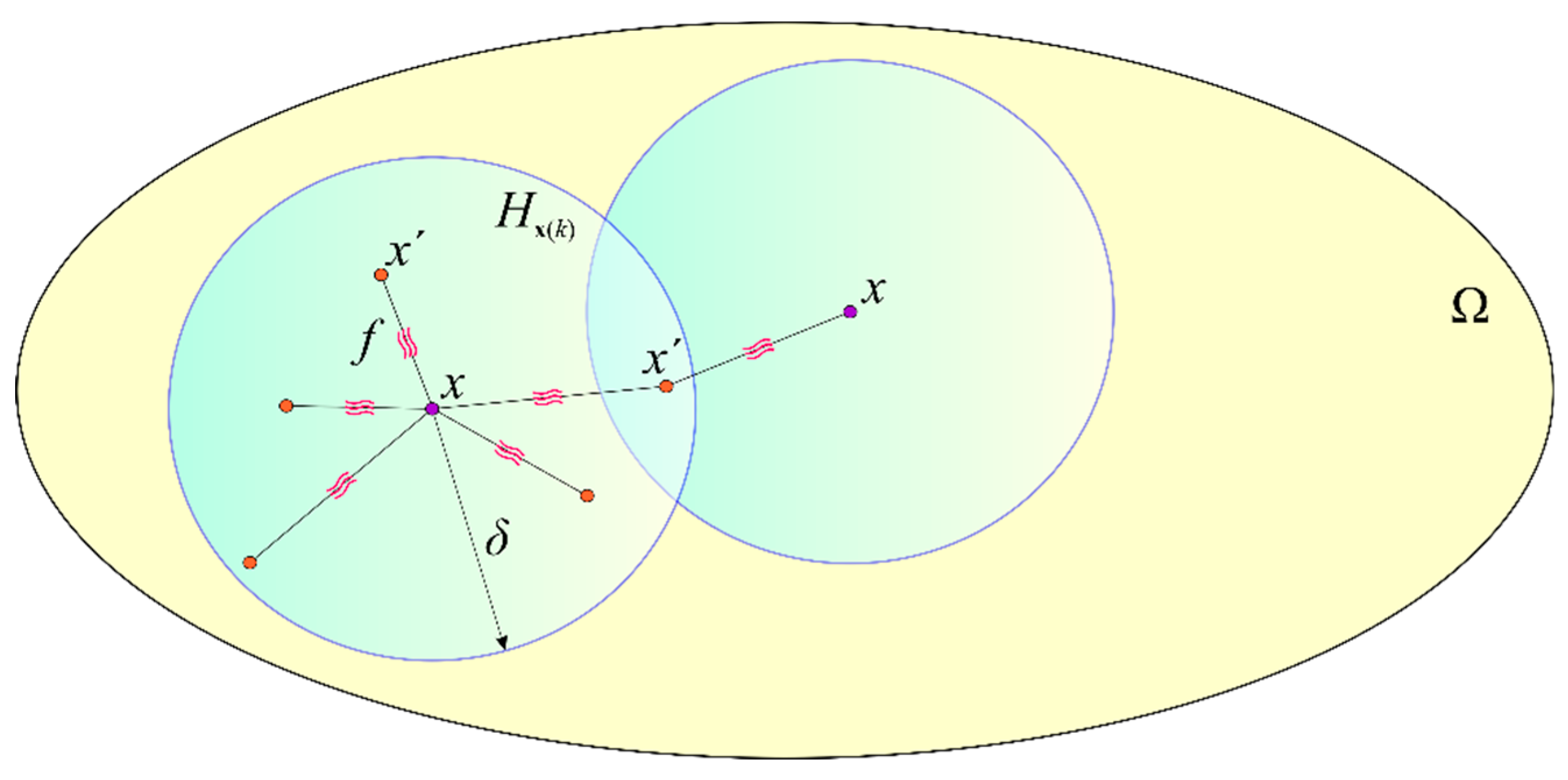
3. Peridynamic Wetness Formulation

The moisture diffusion equation given Equation (2) can be expressed in peridynamic form as [7]

$$\frac{\partial }{\partial t}\left[C_{sat}(t)w(t)\right]={\displaystyle \underset{H}{\int }f\left(w^{\prime },w,x^{\prime },x,t\right)d{V}^{\prime }}+G(t)$$

(14)

where $f\left(w^{\prime },w,x^{\prime },x,t\right)$ is the wetness response function which represents the exchange of moisture between material points $x$ and $x^{\prime }$ that are connected through hygro-bonds, as shown in Figure 1. In PD, material points interact with each other in a nonlocal manner and a material point can interact with other material points within its neighborhood named as the horizon, $H$ (see Figure 1), with a radius of $\delta$.

The wetness response function can be defined as

$$f\left(w^{\prime },w,x^{\prime },x,t\right)=d(t)\frac{w\left(x^{\prime },t\right)-w\left(x,t\right)}{\left|x^{\prime }-x\right|}$$

(15)

where the PD bond parameter, $d(t)$, in Equation (15) can be expressed in terms of the classical diffusivity, $D(t)$, and the saturated concentration, $C_{sat}(t)$, as

$$d=\frac{2D{C}_{sat}}{A{\delta }^2}(1-\mathrm{D}),d=\frac{6D{C}_{sat}}{\pi h{\delta }^3}(2-\mathrm{D})\mathrm{and}d=\frac{6D{C}_{sat}}{\pi {\delta }^4}(3-\mathrm{D}).$$

(16)

In Equation (16), $A$ is the cross-sectional area of a one-dimensional structure and $h$ is the thickness of a two-dimensional structure.

The PD moisture diffusion equation given in Equation (14) can be solved by using the meshless approach. Therefore, the integral term can be replaced by a finite summation and Equation (14) can be rewritten as

$$C_{sat}\frac{\partial w_{\left(k\right)}}{\partial t}={\displaystyle \sum _{j=1}^N{f}_{\left(k\right)\left(j\right)}\left(w_{\left(j\right)},w_{\left(k\right)},x_{\left(j\right)},x_{\left(k\right)},t\right)V_{\left(j\right)}}+G_{\left(k\right)}$$

(17)

with

$$G_{\left(k\right)}=-w_{\left(k\right)}\frac{\partial C_{sat}}{\partial t}$$

(18)

where $w_{(k)}$ and $w_{(j)}$ are wetness values at material points $x_{(k)}$ and $x_{(j)}$, respectively, and $N$ represents the number of material points inside the horizon of the material point $x_{(k)}$. During the solution process for each time step, the time dependency of $C_{sat}$ can be approximated with the backward Euler method between the consecutive time steps as

$$G_{\left(k\right)}=-w_{\left(k\right)}\frac{\Delta C_{sat}}{\Delta t}=-w_{\left(k\right)}\frac{C_{sat}(t+\Delta t)-C_{sat}(t)}{\Delta t}$$

(19)

and an iterative solution is not required to obtain the solution.

4. ANSYS Coupled Field and Diffusion Element Formulations

As mentioned earlier, the commercial finite element software, ANSYS, provides two different types of elements for moisture diffusion analysis. The first type is diffusion (DF) elements, which are available in different forms including Plane 238 (eight-node two-dimensional element), Solid 239 (20-node three-dimensional element), and Solid 240 (10-node three-dimensional element). These elements have only moisture concentration as the degree of freedom (DOF) per node. However, if the saturated moisture concentration, $C_{sat}$, is defined with the command “MP, CSAT” in ANSYS, the DOF becomes the wetness parameter instead of the concentration. The formulation of these elements is based on Equation (11) and they allow the saturated moisture concentration to be a function of time or temperature. However, DF elements are only available for a uniform temperature. If the temperature field is not uniform, ANSYS offers coupled field (CF) elements including Plane 223 (eight-node two-dimensional element), Solid 226 (20-node three-dimensional element), and Solid 227 (10-node three-dimensional element). These elements have two DOFs at each node as wetness, $w$, and temperature, $T$. The formulation of these elements is based on Equation (13). The finite element approximation of field variables for the element e can be expressed as

$$w=S·w_e$$

(20)

and

$$T=S·T_e$$

(21)

where $S$ is the vector of element shape functions, while $T_e$ and $w_e$ represent the vectors of unknown nodal temperature and wetness values of the element. Utilizing the virtual work principle for the element e with the arbitrary virtual quantities of $w_e$ and $T_e$, Equation (13) can be rewritten as

$$C^{dt}{\dot{T}}_e+C^d{\dot{w}}_e=\left(K^d+K_1^{dN}+K_2^{dN}\right)w_e+\left(K^{dtN}+K_1^{dt}+K_2^{dt}+K_2^{dtN}\right)T_e+R$$

(22)

where ${\dot{w}}_e$ and ${\dot{T}}_e$ represent the nodal time derivative of wetness and temperature, respectively. Moreover, $C^d$ is the element diffusion damping matrix, $C^{dt}$ is the element thermal–diffusion damping matrix, $K^d$ is the element diffusion conductivity matrix, $K_1^{dN}$ is the nonlinear part of the element diffusion conductivity matrix associated with thermomigration, $K_2^{dN}$ is the nonlinear part of the element diffusion conductivity matrix due to $\partial C_{sat}/\partial T$, $K^{dtN}$ is the nonlinear part of the element transport conductivity matrix, $K_1^{dt}$ is the element transport conductivity matrix, $K_2^{dt}$ is the element thermal–diffusion conductivity matrix due to $\partial C_{sat}/\partial T$, $K_2^{dtN}$ is the nonlinear part of the element transport conductivity matrix due to $\partial C_{sat}/\partial T$, and $R$ is the nodal diffusion flow rate vector. The explicit definitions of these matrices are given in Reference [14] as

$$C^d=C_{sat}(T){\displaystyle \underset{V_e}{\int }S{S}^{T}dV}$$

(23)

$$C^{dt}=\frac{\partial C_{sat}}{\partial T}{\displaystyle \underset{V_e}{\int }wS{S}^{T}dV}$$

(24)

$$K^d=-D{C}_{sat}(T){\displaystyle \underset{V_e}{\int }{(\nabla S^T)}^T\nabla S^{T}dV}$$

(25)

$$K^{dtN}=-2D{C}_{sat}(T)\frac{Q}{k}{\displaystyle \underset{V_e}{\int }\frac{w}{T^3}{(\nabla S^T)}^T(\nabla T{S}^T)dV}$$

(26)

$$K_1^{dt}=-D{C}_{sat}(T)\frac{Q}{k}{\displaystyle \underset{V_e}{\int }\frac{w}{T^2}{(\nabla S^T)}^T\nabla S^{T}dV}$$

(27)

$$K_1^{dN}=D{C}_{sat}(T)\frac{Q}{k}{\displaystyle \underset{V_e}{\int }\frac{1}{T^2}{(\nabla S^T)}^T(\nabla T{S}^T)dV}$$

(28)

$$K_2^{dt}=-D\frac{\partial C_{sat}}{\partial T}{\displaystyle \underset{V_e}{\int }w{(\nabla S^T)}^T\nabla S^{T}dV}$$

(29)

$$K_2^{dN}=D\frac{\partial C_{sat}}{\partial T}{\displaystyle \underset{V_e}{\int }[{(\nabla S^T)}^T(S{(\nabla T)}^T)+{(\nabla S^T)}^T(\nabla T{S}^T)]dV}$$

(30)

$$K_2^{dtN}=D\frac{\partial C_{sat}}{\partial T}\frac{Q}{k}{\displaystyle \underset{V_e}{\int }\frac{w}{T^2}{(\nabla S^T)}^T(\nabla T{S}^T)dV}$$

(31)

$$R=G{\displaystyle \underset{V_e}{\int }SdV}$$

(32)

where $V_e$ is the volume of the element. Utilizing Equation (22), the coupled finite element thermal–diffusion matrix equations can be written as

$$\left[\begin{array}{cc}{C}^t& 0\\ C^{dt}& C^d\end{array}\right]\left\{\begin{array}{c}{\dot{T}}_e\\ {\dot{w}}_e\end{array}\right\}+\left[\begin{array}{cc}{K}^t& 0\\ (K_1^{dt}+K^{dtN}+K_2^{dtN}+K_2^{dt})& (K^d+K_1^{dN}+K_2^{dN})\end{array}\right]\left\{\begin{array}{c}{T}_e\\ w_e\end{array}\right\}=\left\{\begin{array}{c}Q\\ R\end{array}\right\}$$

(33)

where $C^t$, $K^t$, and $Q$ represent the element specific heat matrix, the element thermal conductivity matrix, and the element heat generation load matrix, respectively. The thermal conductivity matrix, $K^t$, is a combination of the element mass transport conductivity matrix, $K^{tm}$, the element diffusion conductivity matrix, $K^{tb}$, and the element convection surface conductivity matrix, $K^{tc}$. If thermomigration is negligible, Equation (33) can be simplified as

$$\left[\begin{array}{cc}{C}^t& 0\\ C^{dt}& C^d\end{array}\right]\left\{\begin{array}{c}{\dot{T}}_e\\ {\dot{w}}_e\end{array}\right\}+\left[\begin{array}{cc}{K}^t& 0\\ K_2^{dtN}& (K^d+K_2^{dN})\end{array}\right]\left\{\begin{array}{c}{T}_e\\ w_e\end{array}\right\}=\left\{\begin{array}{c}Q\\ R\end{array}\right\}.$$

(34)

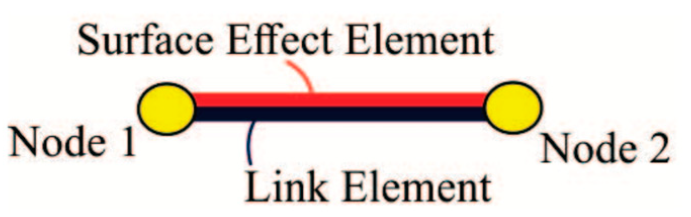
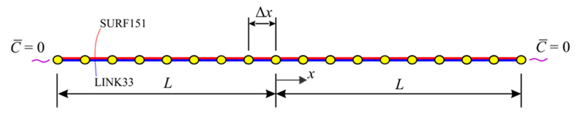
5. ANSYS Thermal and Surface Effect Element Formulations

In addition to elements provided by ANSYS described in the previous section for moisture diffusion modeling, an alternative approach is presented in this study by utilizing conventional thermal and surface effect elements. Utilizing the virtual work principle in conjunction with the divergence theorem, Fick’s second law equation given in Equation (6) can be written as

$$\begin{array}{l}\delta w{\displaystyle \underset{V_e}{\int }{C}_{sat}(t)\frac{\partial w}{\partial t}dV}+\delta w{\displaystyle \underset{V_e}{\int }w\frac{\partial C_{sat}}{\partial t}dV}=\\ -D(t)C_{sat}(t){\displaystyle \underset{V_e}{\int }\nabla (\delta w)\nabla wdV}+D(t)C_{sat}(t)\delta w{\displaystyle \underset{V_e}{\int }G(x,t)dV}+\delta w{\displaystyle \underset{S_e}{\int }\nabla wndS}\end{array}$$

(35)

where $S_e$ and $n$ represent the surface of the element and unit normal vector to this surface, respectively. In Equation (35), the time derivative of the saturated concentration, i.e., $d{C}_{sat}/dt$, can be expressed by using backward Euler method as

$$H=w\frac{\Delta C_{sat}}{\Delta t}.$$

(36)

After substituting the wetness field expression, $w$, given in Equation (20) into Equation (35) for arbitrary $\delta w_e$, Equation (35) can be written in a matrix form as

$$(C^{dt}+C^d){\dot{w}}_e+K^d{w}_e=R$$

(37)

where

$$C^d=C_{sat}(t){\displaystyle \underset{V_e}{\int }S{S}^{T}dV}$$

(38)

$$K^d=D{C}_{sat}(t){\displaystyle \underset{V_e}{\int }{(\nabla S^T)}^T\nabla S^{T}dV}$$

(39)

$$C^{dt}=\frac{\partial C_{sat}}{\partial t}{\displaystyle \underset{V_e}{\int }S{S}^{T}dV}$$

(40)

$$R=G{\displaystyle \underset{V_e}{\int }SdV}.$$

(41)

Note that this equation has the same form as the heat flow equation, which can be written as

$$C_e^t{\dot{T}}_e+(K_e^{tb}+K_e^{tc})T_e=Q_e^g$$

(42)

where

$$C_e^t=\rho c{\displaystyle \underset{V}{\int }S{S}^T}dV$$

(43)

$$K_e^{tb}=D_t{\displaystyle \underset{V}{\int }{(\nabla S^T)}^T\nabla S^{T}dV}$$

(44)

$$K_e^{tc}=h_f{\displaystyle \underset{S}{\int }S{S}^{T}dS}$$

(45)

$$Q_e^g=\overline{q}{\displaystyle \underset{V}{\int }SdV}$$

(46)

where $\rho$, $c$, $D(t)$, $h_f$, and $\overline{q}$ represent the density, the specific heat, the thermal conductivity, the film coefficient, and the heat generation rate per unit volume, respectively. Since the wetness and heat flow equations given in Equations (37) and (42) have the same form, it is possible to relate the thermal parameters, $\rho$, $c$, $D_t$, $h_f$, and $\overline{q}$ to diffusion parameters $C_{sat}(t)$, $D{C}_{sat}(t)$, $\partial C_{sat}/\partial t$, and G. Therefore, for one-dimensional analysis, the wetness field equation given in Equation (37) can be made equivalent to the thermal heat flow equation given in Equation (42) by using a combination of thermal link (LINK33) and thermal surface effect (SURF151) elements between two nodes (see Figure 2) and adjusting parameters as demonstrated in

Table 1. The relationship between thermal and diffusion parameters for the thermal link element, LINK33.

		LINK33
Material Properties		Original	Modified	ANSYS Command
	Thermal Conductivity	$D_t$	$D_{n+1}{C}_{sat,n+1}$	MP, KXX, MAT 1, $D_{n+1}{C}_{sat,n+1}$
	Density	$\rho$	1.0	MP, DENS, MAT 1, 1.0
	Specific Heat	c	$C_{sat,n+1}$	MP, C, MAT 1, $C_{sat,n+1}$
Real Constants	Cross Sectional Area	A	A	R, NSET 2, A

¹ MAT: Material reference number, ² NSET: Real constant set identification number.

and

Table 2. The relationship between thermal and diffusion parameters for surface effect element, SURF151.

		SURF151
Applying Surface loads on elements (SFE)	Convection (CONV)	Original	Modified	ANSYS Command
	Film Coefficient	$h_f$	$\frac{\Delta C_{sat}A}{\Delta t}$	SFE, Elem 1, CONV, 1, $\frac{\Delta C_{sat}A}{\Delta t}$
	Bulk Temperature	$T_B$	0.0	SFE, Elem 1, CONV, 2, 0.0

¹ Elem: Element to which surface load applies.

. Note that the thermal link element is necessary to construct $C_e^t$ and $K_e^{tb}$ matrices and the thermal surface effect element is necessary to construct the $K_e^{tc}$ matrix. In Table 1, the subscript n in $D_{n+1}$ and $C_{sat,n+1}$ represents the current time step number. In Table 2, the rate of $C_{sat}$ can be approximated with the backward Euler method as $\Delta C_{sat}/\Delta t$, in which Δ implies the difference of values between the time steps. Moreover, the nodal heat generation rate per unit volume, $\overline{q}$, can be used in place of the diffusing substance generation rate per unit volume, G, in ANSYS by defining the nodal loads with the “BF, Node, HGEN, Value” command.

6. Numerical Results

In this section, numerical results for the analysis of the desorption process in a bar during reflow soldering are presented by considering conventional thermal link and surface effect elements, diffusion (DF) and coupled field (CF) elements, and peridynamics. The two-material bar shown in Figure 3 is initially fully saturated at 85 °C/100% RH with isolated lateral surfaces. The material properties for diffusion and thermal analyses are given in

Table 3. Material properties for materials 1 and 2 for diffusion analysis.

	Material 1	Material 2
Diffusivity factor, $D_0$ (${\mathrm{m}}^2/\mathrm{s}$)	$5\times {10}^{-3}$	$4\times {10}^{-3}$
Solubility factor, $S_0$ $({\mathrm{kg}/\mathrm{m}}^3\mathrm{Pa})$	$6\times {10}^{-10}$	$2\times {10}^{-10}$
Pressure factor, $P_0$ ($\mathrm{Pa}$)	$5.0492\times {10}^{10}$	$5.0492\times {10}^{10}$
Diffusion activation energy, $E_D$ ($\mathrm{J}/\mathrm{mol}$)	$5\times {10}^4$	$5\times {10}^4$
Solubility activation energy, $E_S$ ($\mathrm{J}/\mathrm{mol}$)	$4\times {10}^4$	$4\times {10}^4$
Vapor pressure activation energy, $E_{VP}$ ($\mathrm{J}/\mathrm{mol}$)	$4.08737\times {10}^4$	$4.08737\times {10}^4$

and

Table 4. Material properties for materials 1 and 2 for thermal analysis.

	Material 1	Material 2
Density, $\rho$ (${\mathrm{kg}/\mathrm{m}}^3$)	$3\times {10}^3$	$3\times {10}^3$
Specific Heat, $c$ ($\mathrm{J}/\mathrm{kgK}$)	$1.5\times {10}^3$	$1.5\times {10}^3$
Thermal Conductivity, $k$ ($\mathrm{W}/\mathrm{mK}$)	$0.2$	$0.6$

based on the data provided in Reference [15].

The initial and boundary conditions of the wetness field are specified as

$$w(x,t=0)=1\mathrm{with}-L\le x\le L$$

(47)

$$w(x=\pm L,t)=0$$

(48)

$$\frac{\partial w}{\partial y}(x,y=\pm h/2)=0\mathrm{with}-h/2\le y\le h/2$$

(49)

where 2L and h represent the length and thickness of the bar, respectively. The solubility activation energy of materials 1 and 2 are either equal or unequal at the interface. The time-dependent saturated concentration, $C_{sat}(t)$, and diffusivity, $D(t)$, can be expressed as

$$D(t)=D_0{e}^{\left(\frac{-E_D}{RT(t)}\right)}$$

(50)

and

$$C_{sat}\left(t\right)=S_0{P}_0{e}^{\left(\frac{E_S-E_{VP}}{RT\left(t\right)}\right)}\times RH$$

(51)

where R is the universal gas constant ($R=8.3145\mathrm{J}/\mathrm{Kmol}$), $D_0$ is the diffusivity factor, $S_0$ is the solubility factor, $P_0$ is the pressure factor, $E_D$ is the activation energy of the diffusivity, $E_S$ is the activation energy of the solubility, $E_{VP}$ is the vapor pressure activation energy, and RH indicates the relative humidity.

For CF elements, the saturated concentration, $C_{sat}(T)$ can be specified as temperature-dependent. On the other hand, the diffusivity can be specified as either time-dependent, $D(t)$, or temperature-dependent, $D(T)$. Moreover, the temperature field can be either uniform or nonuniform. However, the DF element is not suitable for nonuniform temperature conditions since the temperature is not known a priori. In addition, the solutions with diffusion and coupled field elements are obtained by neglecting transport velocity and thermomigration, respectively.

The finite element (FE) discretization of a bar with conventional thermal elements (present approach) and with two-dimensional DF or CF elements are shown in Figure 4 and Figure 5, respectively. The bar has a length of $2L=2\mathrm{mm}$, thickness of $h=L/100$, and cross-sectional area of $A=h^2$. The discretization size is specified as $\Delta x=h$. The total time is specified as $t=80\mathrm{s}$ with a time step size of $\Delta t=2\mathrm{s}$. The moisture concentration results are plotted at four different time instances, t = 20, 40, 60, and 80 s. The results obtained from the current approach are compared against peridynamics as well as ANSYS DF and CF element results for uniform and nonuniform temperature conditions with equal and unequal solubility activation energies of materials 1 and 2. In the case of unequal solubility activation energy, material 2 has $E_{S_2}=4.50\times {10}^4\mathrm{J}/\mathrm{mol}$.

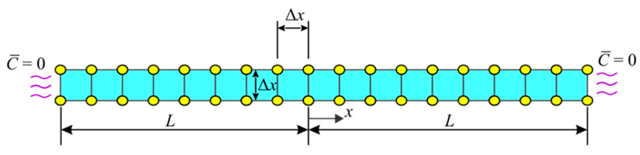
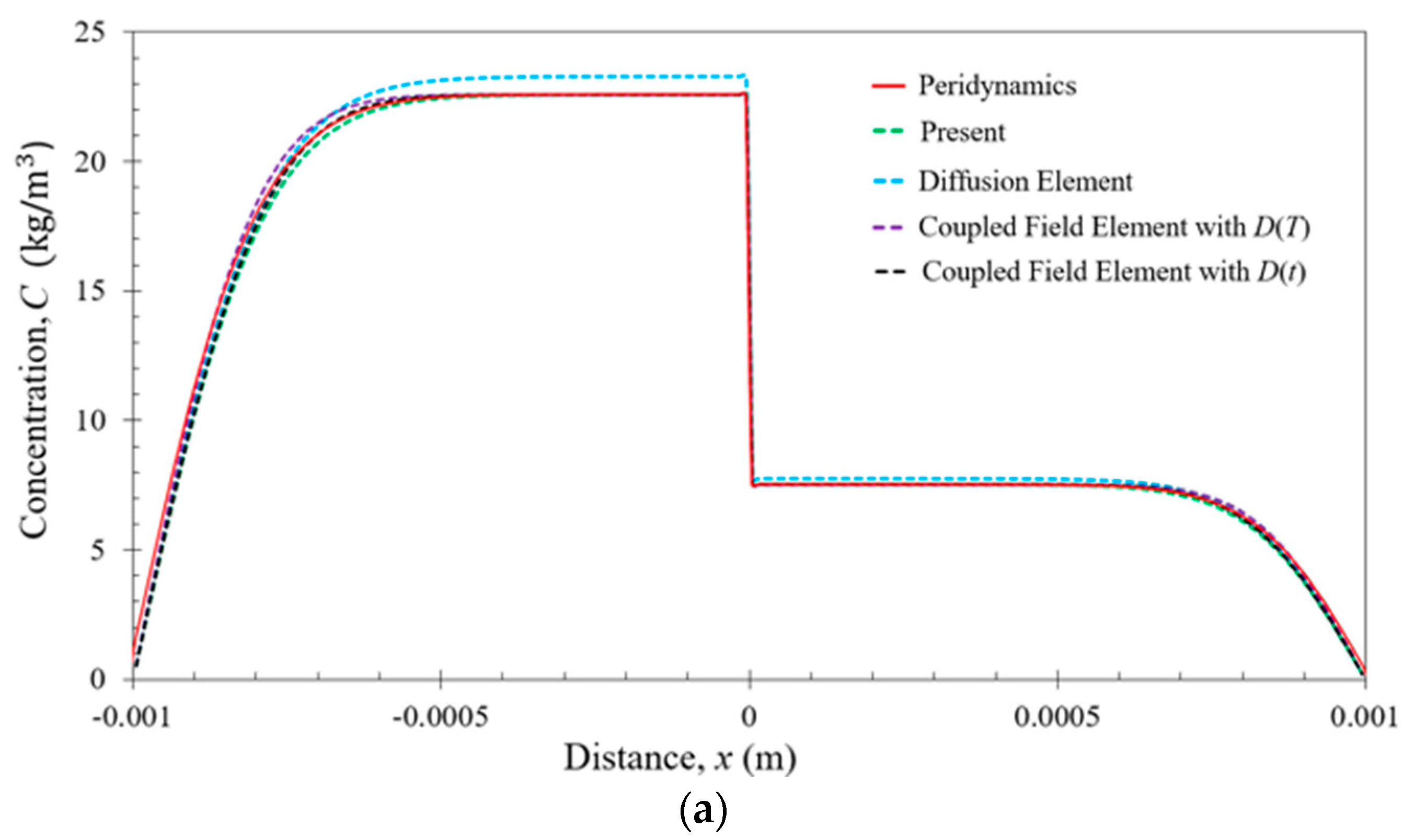
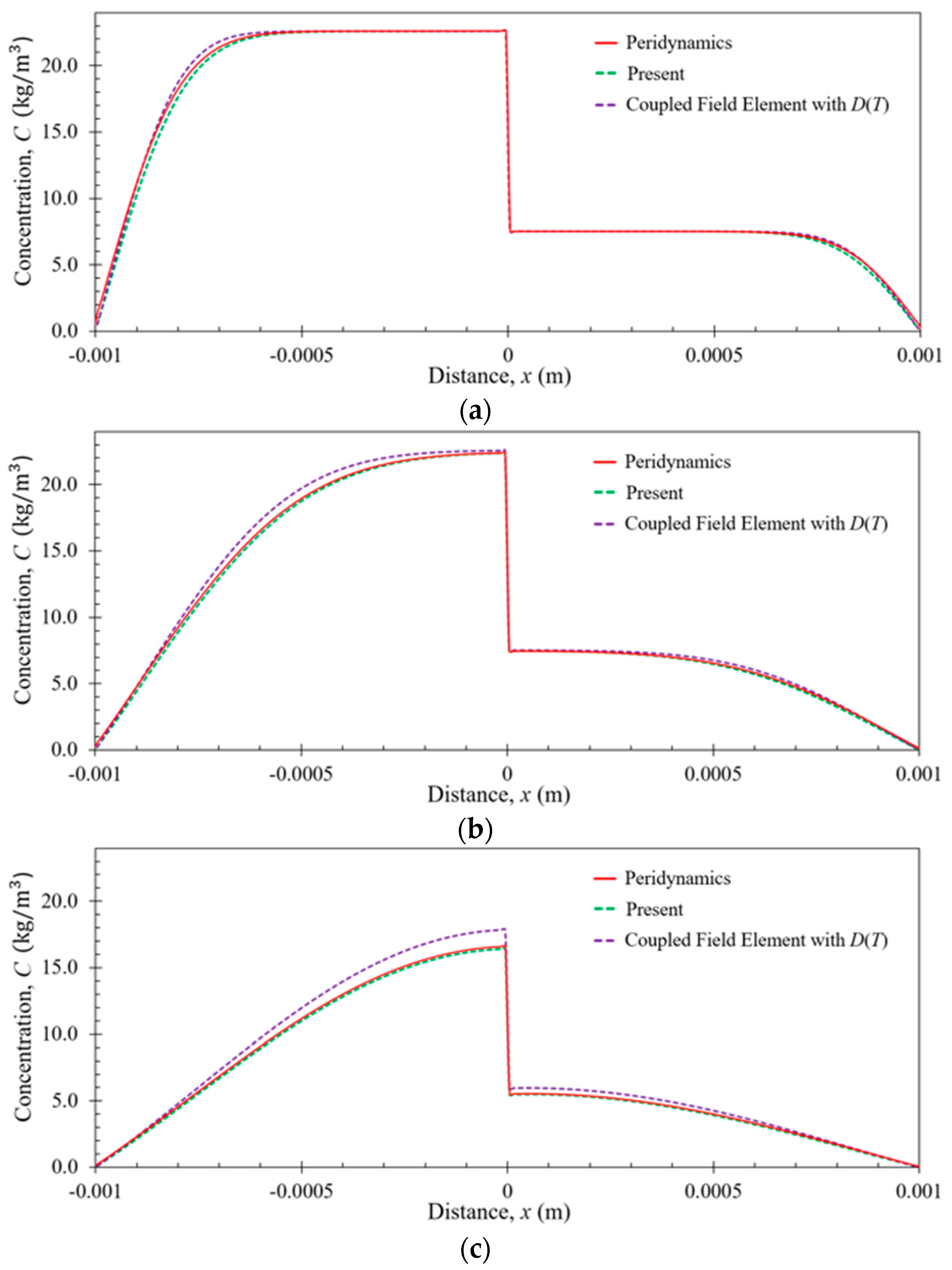
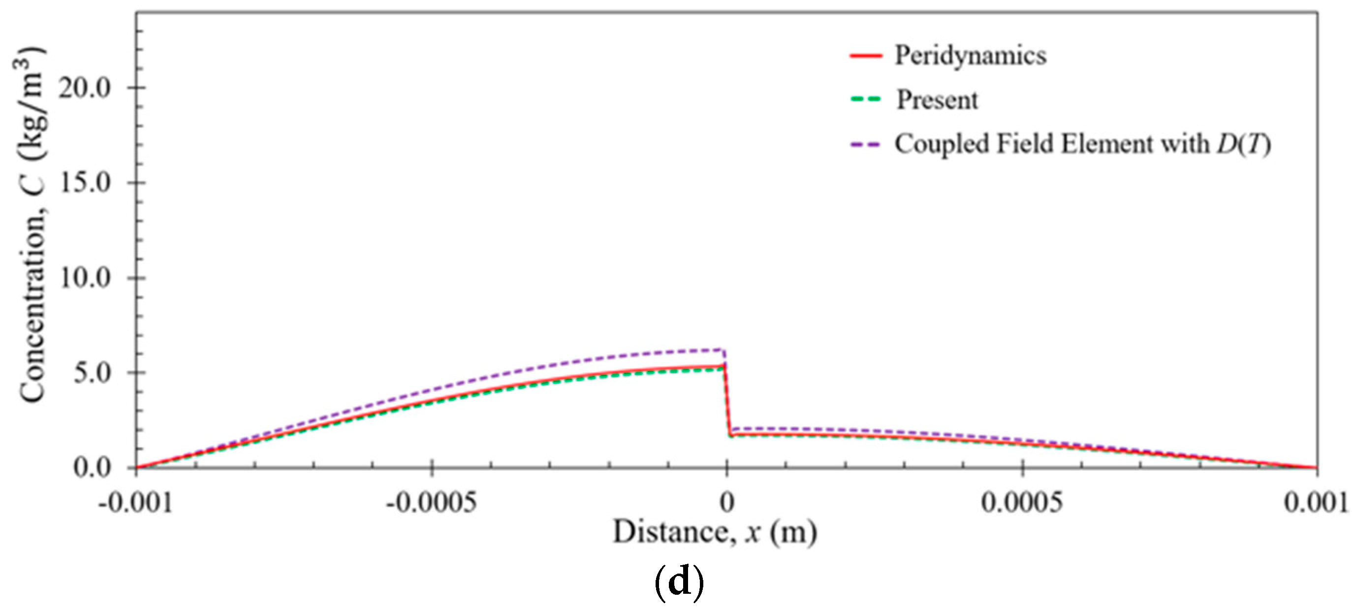
6.1. Bar Subjected to Uniform Temperature

In the first case, the two-material bar configuration is subjected to the uniform temperature field of

$$T(x,t)=\left(85+2t\right)°\mathrm{C}.$$

(52)

As shown in Figure 6 and Figure 7, the predictions based on the present approach, CF elements with time-dependent diffusivity, $D(t)$, and temperature-dependent saturated concentration, $C_{sat}(T)$, and peridynamics are in excellent agreement for both equal and unequal values of $E_S$ under uniform temperature conditions. However, the CF elements with temperature-dependent diffusivity, $D(T)$, and saturated concentration, $C_{sat}(T)$, and the DF elements show significant deviation from the other solutions. When diffusivity is imposed as a time-dependent property, $D(t)$, its value is known before the next time step as part of time integration, and does not require approximation. However, if temperature-dependent diffusivity, $D(T)$, is considered, this requires approximation for the next time step. Therefore, this will yield results significantly different from the correct solution. Moreover, the DF elements do not predict the correct concentration because they disregard the effect of the time derivative of the saturated concentration.

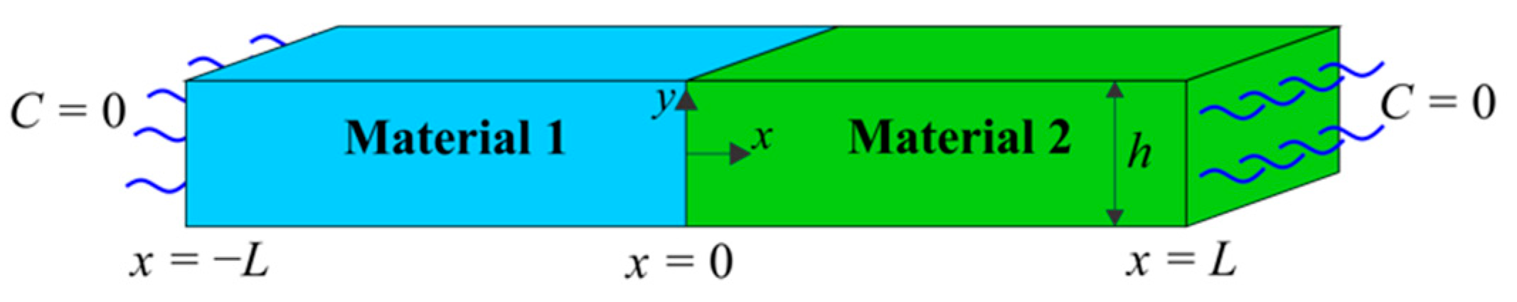
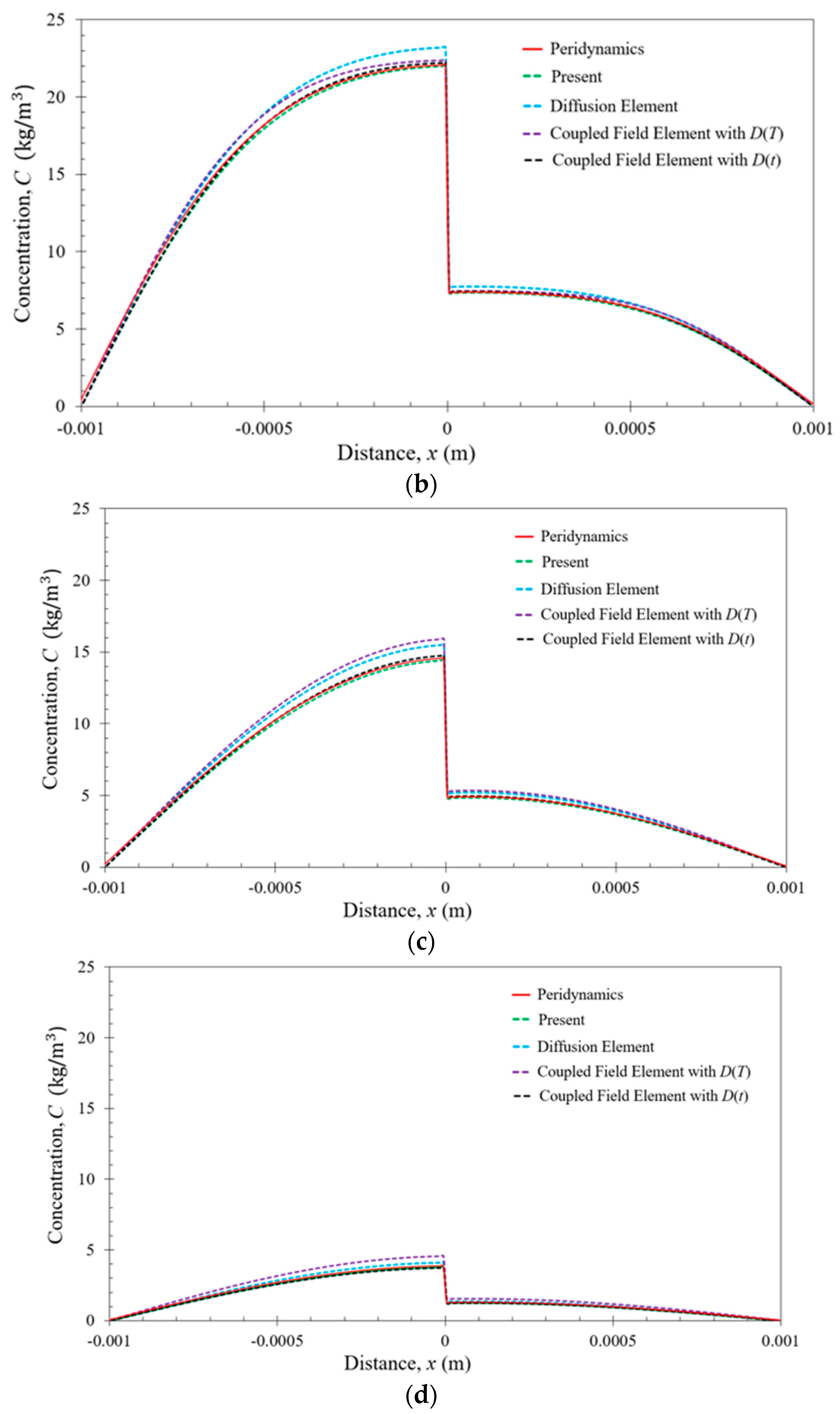
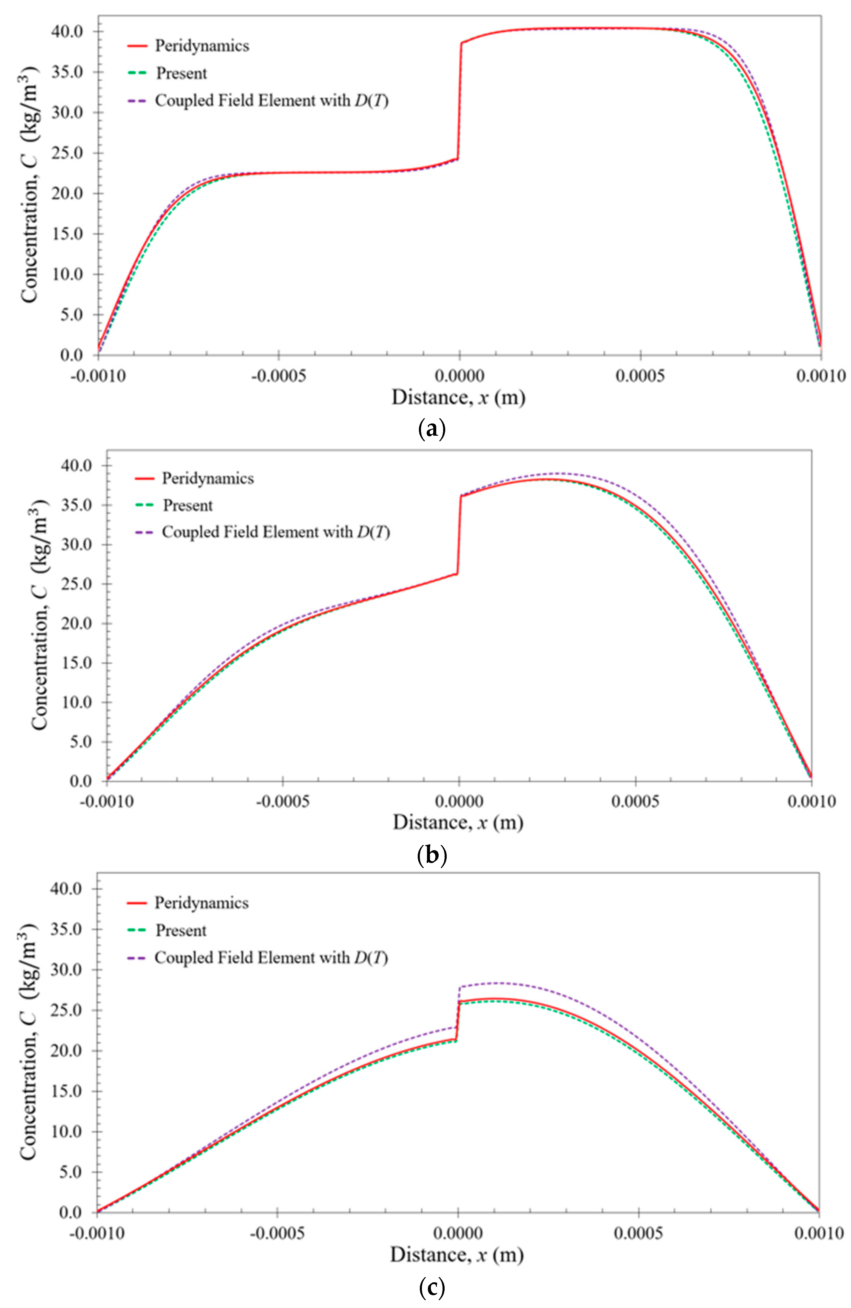
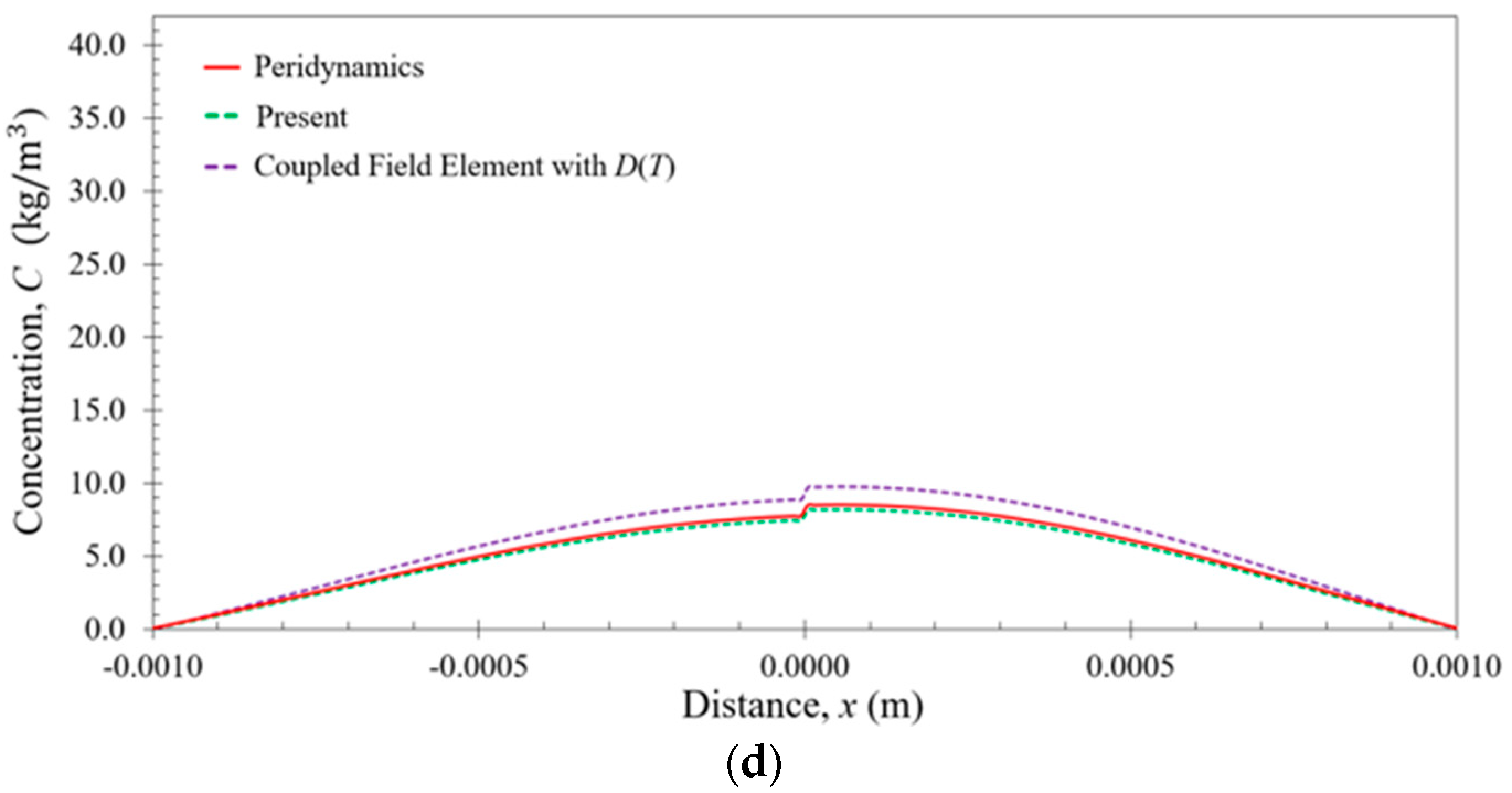
6.2. Bar Subjected to Nonuniform Temperature

In the second case, a nonuniform temperature condition is considered. The nonuniform temperature is obtained by applying the temperature boundary conditions in the form of

$$T(x=\pm L,t)=\left(85+2t\right)°\mathrm{C}.$$

(53)

The DF element is not applicable due to the nonuniformity of the temperature field. Moreover, the CF element with time-dependent diffusivity, $D(t)$, is also not applicable because diffusivity, $D(t)$, given in Equation (50), highly depends on temperature which is the unknown DOF in this problem. The concentration results along the bar are plotted in Figure 8 and Figure 9. As can be seen from these figures, the predictions from the present approach and peridynamics are in very good agreement, whereas there is a significant difference between the results from the CF elements with temperature dependence, $D(T)$.

7. Conclusions

This study presents a new finite element-based modeling approach for moisture diffusion analysis in the presence of time-dependent saturated moisture concentration by utilizing conventional ANSYS thermal and surface effect elements. The capability of the present approach is demonstrated by comparing results from the present approach with those obtained using ANSYS diffusion and coupled field elements as well as peridynamic theory. For comparison purposes, a fully saturated one-dimensional two-material bar configuration is considered with either the same or different solubility activation energies in the presence of a time-dependent saturated moisture concentration. Both uniform and nonuniform temperature conditions are analyzed. For all cases, the current approach is capable of predicting correct concentration values. This is not true for ANSYS diffusion and coupled field elements. If the diffusivity is a function of temperature, coupled field elements could not provide an accurate solution. On the other hand, although the diffusion element is shown to be suitable for a uniform temperature, it can yield incorrect results, especially for unequal values of solubility activation energies in a multi-material system. As a summary, the present approach is superior to the diffusion and coupled field elements of ANSYS, especially under nonuniform temperature conditions.

References

1. Wong, E.H.; Park, B. Moisture diffusion modeling—A critical review. Microelectron. Reliab. 2016, 65, 318–326. [Google Scholar] [CrossRef]
2. Wong, E.H.; Teo, Y.C.; Lim, T.B. Moisture diffusion and vapor pressure modeling of IC packaging. In Proceedings of the 48th Electronic Components and Technology Conference, Seattle, WA, USA, 25–28 May 1998; pp. 1372–1378. [Google Scholar]
3. Yoon, S.; Han, B.; Wang, Z. On moisture diffusion modeling using thermal-moisture analogy. ASME J. Electron. Packag. 2007, 129, 421–426. [Google Scholar] [CrossRef]
4. Jang, C.; Park, S.; Han, B.; Yoon, S. Advanced thermal-moisture analogy scheme for anisothermal moisture diffusion problem. ASME J. Electron. Packag. 2008, 130, 011004. [Google Scholar] [CrossRef]
5. Wong, E.H.; Koh, S.W.; Lee, K.H.; Rajoo, R. Advanced moisture diffusion modeling & characterization for electronic packaging. In Proceedings of the 52nd Electronic Components and Technology Conference, San Diego, CA, USA, 28–31 May 2002; pp. 1297–1303. [Google Scholar]
6. Wong, E.H. The fundamentals of thermal-mass diffusion analogy. Microelectron. Reliab. 2015, 55, 588–595. [Google Scholar] [CrossRef]
7. Diyaroglu, C.; Oterkus, S.; Oterkus, E.; Madenci, E.; Han, S.; Hwang, Y. Peridynamic wetness approach for moisture concentration analysis in electronic packages. Microelectron. Relia. 2017, 70, 103–111. [Google Scholar] [CrossRef] [Green Version]
8. Diyaroglu, C.; Oterkus, S.; Oterkus, E.; Madenci, E. Peridynamic modeling of diffusion by using finite element analysis. IEEE Trans. Compon. Packag. Manuf. Technol. 2017, 7, 1823–1831. [Google Scholar] [CrossRef]
9. Chen, L.; Liu, Y.; Fan, X. Application of water activity-based theory for moisture diffusion in electronic packages using ANSYS. In Proceedings of the 19th International Conference on Thermal, Mechanical and Multi-Physics Simulation and Experiments in Microelectronics and Microsystems, Toulouse, France, 15–18 April 2018; pp. 1–6. [Google Scholar]
10. Chen, L.; Zhou, J.; Chu, H.W.; Zhang, G.; Fan, X. Modeling nonlinear moisture diffusion in inhomogeneous media. Microelectron. Reliab. 2017, 75, 162–170. [Google Scholar] [CrossRef]
11. Liu, D.; Park, S. A note on the normalized approach to simulating moisture diffusion in a multimaterial system under transient thermal conditions using ANSYS 14 and 14.5. ASME J. Electron. Packag. 2014, 136, 034501. [Google Scholar] [CrossRef]
12. Sutton, M. Moisture Diffusion Modeling with ANSYS at R14 and Beyond. Available online: http://www.padtinc.com/blog/wp-content/uploads/oldblog/PADT-Webinar-Moisture-Diffusion-2012_05_24.pdf (accessed on 9 December 2018).
13. Diyaroglu, C.; Madenci, E.; Oterkus, S.; Oterkus, E. A novel finite element technique for moisture diffusion modeling using ANSYS. In Proceedings of the 68th Electronic Components and Technology Conference, San Diego, CA, USA, 29 May–1 June 2018; pp. 227–235. [Google Scholar]
14. ANSYS 19.0 Mechanical User’s Guide; ANSYS: Canonsburg, PA, USA, 2018.
15. Wang, J.; Liu, R.; Liu, D.; Park, S. Advancement in simulating moisture diffusion in electronic packages under dynamic thermal loading conditions. Microelectron. Reliab. 2017, 73, 42–53. [Google Scholar] [CrossRef]
Figure 1. Horizon of the material point x and its interaction with neighboring points, x .
Electronics 07 00438 g001
Figure 2. Current approach by combining thermal link and surface effect elements between two nodes.
Electronics 07 00438 g002
Figure 3. Two-material bar configuration in the desorption process.
Electronics 07 00438 g003
Figure 4. The finite element discretization of a bar for the present approach.
Electronics 07 00438 g004
Figure 5. The finite element discretization of a bar for “diffusion” or “coupled field” elements.
Electronics 07 00438 g005
Figure 6. Variation of moisture concentration along the bar at t = (a) 20 s; (b) 40 s; (c) 60 s; and (d) 80 s with equal E S values for materials 1 and 2.
Electronics 07 00438 g006aElectronics 07 00438 g006b
Figure 7. Variation of moisture concentration along the bar at t = (a) 20 s; (b) 40 s; (c) 60 s; and (d) 80 s with unequal E S for materials 1 and 2.
Electronics 07 00438 g007
Figure 8. Variation of moisture concentration along the bar at t = (a) 20 s; (b) 40 s; (c) 60 s; and (d) 80 s with equal E S values for materials 1 and 2.
Electronics 07 00438 g008aElectronics 07 00438 g008b
Figure 9. Variation of moisture concentration along the bar at t = (a) 20 s; (b) 40 s; (c) 60 s; and (d) 80 s with unequal E S for materials 1 and 2.
Electronics 07 00438 g009aElectronics 07 00438 g009b