Planar Array Diagnostic Tool for Millimeter-Wave Wireless Communication Systems

Abstract

In this paper, a diagnostic tool or procedure based on Bayesian compressive sensing (BCS) is proposed for identification of failed element(s) which manifest in millimeter-wave planar antenna arrays. With adequate a priori knowledge of the reference antenna array radiation pattern, a diagnostic problem of faulty elements was formulated. Sparse recovery algorithms, including total variation (TV), mixed ${\ell }_1/{\ell }_2$ norm, and minimization of the ${\ell }_1$, are readily available in the literature, and were used to diagnose the array under test (AUT) from measurement points, consequently providing faster and better diagnostic schemes than the traditional mechanisms, such as the back propagation algorithm, matrix method algorithm, etc. However, these approaches exhibit some drawbacks in terms of effectiveness and reliability in noisy data, and a large number of measurement data points. To overcome these problems, a methodology based on BCS was adapted in this paper. From far-field radiation pattern samples, planar array diagnosis was formulated as a sparse signal recovery problem where BCS was applied to recover the locations of the faults using relevance vector machine (RVM). The resulted BCS approach was validated through simulations and experiments to provide suitable guidelines for users, as well as insight into the features and potential of the proposed procedure. A Ka-band $\left(28.9\mathrm{GHz}\right)$ $10\times 10$ rectangular microstrip patch antenna array that emulates failure with zero excitation was designed for far-field measurements in an anechoic chamber. Both simulated and measured far-field samples were used to test the proposed approach. The proposed technique is demonstrated to detect diagnostic problems with fewer measurements provided the prior knowledge of the array radiation pattern is known, and the number of faults is relatively smaller than the array size. The effectiveness and reliability of the technique is verified experimentally and via simulation. In addition to a faster diagnosis and better reconstruction accuracy, the BCS-based technique shows more robustness to additive noisy data compared to other compressive sensing methods. The proposed procedure can be applied to next-generation transceivers, aerospace systems, radar systems, and other communication systems.

1. Introduction

Antenna array is a key technology component in various communication systems such as radar, radio-astronomy, remote sensing, satellite communications, and next-generation (fifth generation, 5G) wireless communications [1], where a very large number (in the hundreds) of radiating elements are particularly used to meet the increasing demands of high radiation performance and reconfigurability [2]. Conversely, the higher the number of radiating elements in the beam-forming configuration, the higher the probability of failed element(s) will be. This causes abrupt field variations across the aperture of the array, and distortion in the radiation features (e.g., beamwidth, peak sidelobe, and boresight). Therefore, the availability of reliable and effective diagnosis tools for large arrays remains an asset, because manual dismantling and replacement operations consume excessive time and cost, and are even unfeasible in satellite-borne installations. Currently, failure identification in antenna arrays is a theoretical and practical important research domain. Detection of faulty elements in antenna arrays is of great interest in both military and civilian markets. 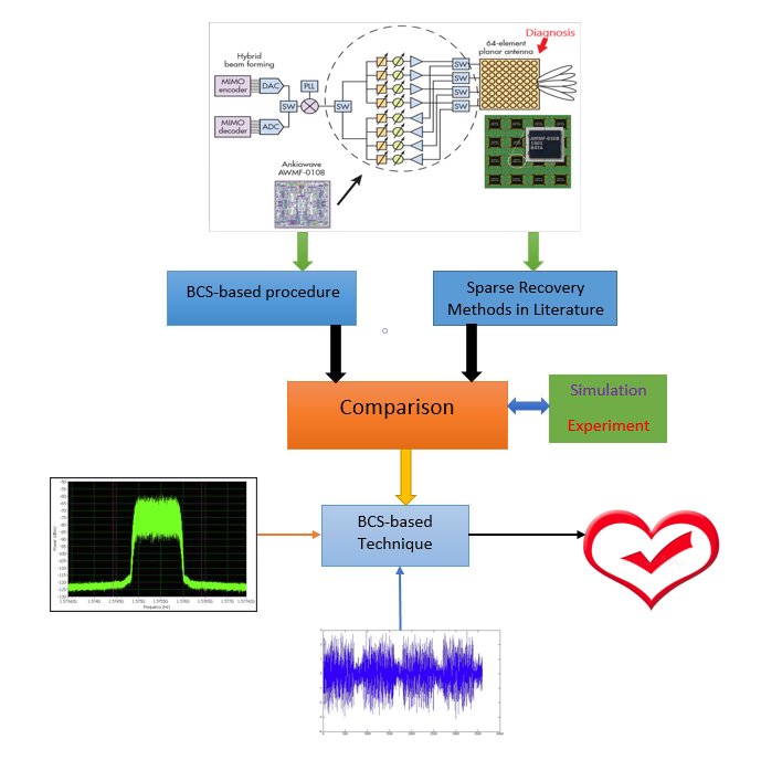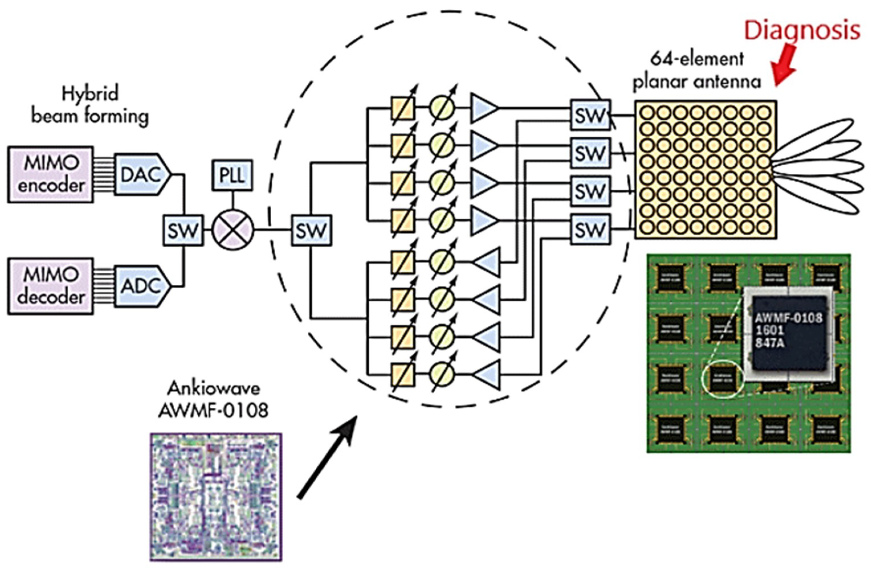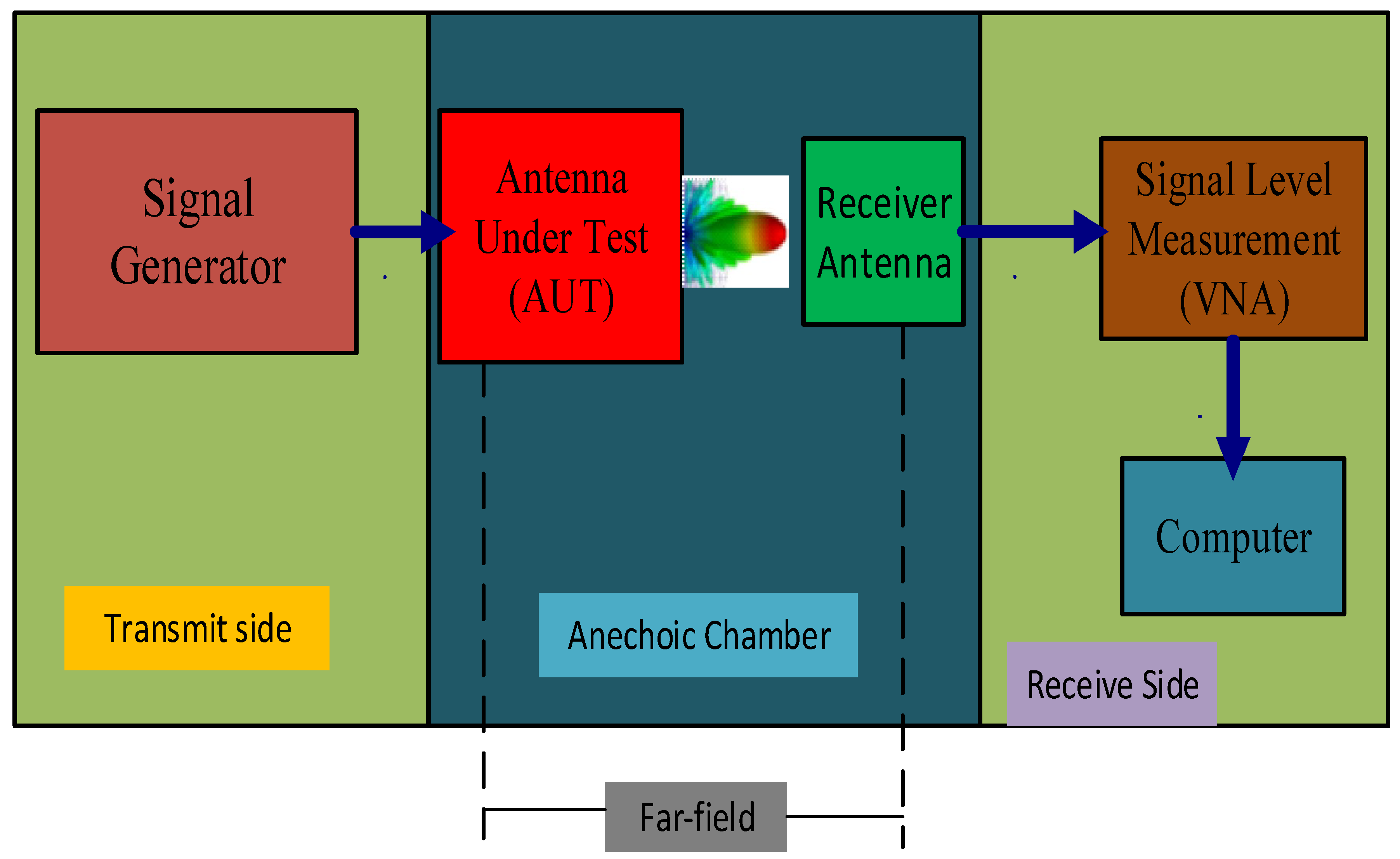Upcoming technologies adopt active or passive antenna arrays with a large number of elements [1,2,3,4,5]. For instance, millimeter-wave transceivers implement multiple-input multiple-output (MIMO) features and beamforming for future 5G applications, as shown in Figure 1. The block diagram shows the location of the AWMF-0108 in a 5G MIMO system [6]. The integrated circuit (IC) contents in the circle are the gain and phase control blocks with amplification and RX/TX switching. The first industrial and commercial millimeter-wave quad-core IC transceiver for 5G applications is the AWMF-0108 [6]. Many compactable antennas were designed for that purpose. Thus, some communication systems will evolve for 5G technology, even before full deployment, which is not expected until 2020. The large number of elements in the planar antenna required by the transceiver must function optimally. Failure in the element(s) causes far-field degradation of antenna systems. The detection of failed elements from field measurements taken from a suitable observation point is very important to re-calibrate the feeding network and to reinstall the needed radiation characteristics by reconfiguring the excitations of the healthy elements [1,3]. Testing of antennas is then a necessity when a certain number of elements exhibit fault. Therefore, the fast diagnosis of complex antenna structures is always a fundamental need.

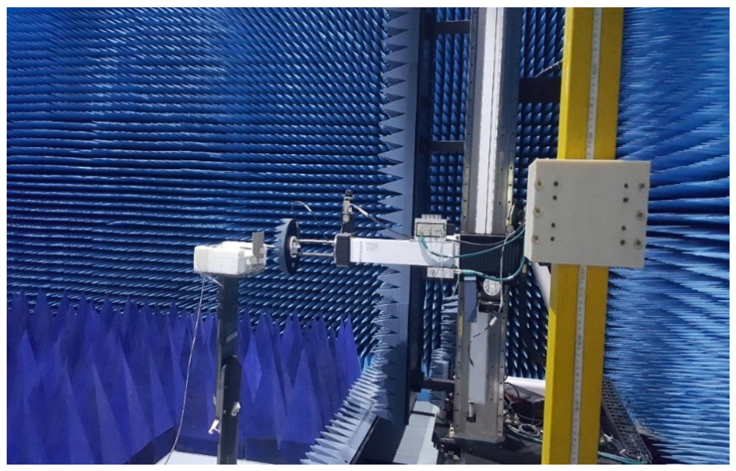
Far-field measurements are a very powerful approach for antenna array testing. The measurement data are sequentially presented for probable failure identification in the array under test (AUT). The matrix method algorithm (MMA) and back propagation algorithm (BPA) are the most commonly used mechanisms to detect the number and corresponding positions of defective elements using a reference antenna (healthy) and the AUT (defective). BPA [7] was established using the Fourier relationship between radiated far-field and the field situated on the array aperture, and it is applicable to planar antenna arrays. A generalized form of BPA is MMA [8,9]. MMA uses linear algebra standard tools to stabilize the inversion matrix, which relates the array aperture field to radiated far-field. However, MMA and BPA demand a large number of measurements, thus causing long post-processing of large arrays. One approach to mitigate the problem is the use of a priori knowledge of the array without failure; consequently, only the defective array elements are identified. The modeled diagnostic problem is solved by employing available customs whose computation time is a little longer than standard methodologies. At this point, it is evident that the total time taken to get the antenna array diagnosed greatly depends on measurement time, with post-processing times having a higher order of magnitude. This is why sparse recovery-based methods require fewer measurement numbers and provide faster antenna array diagnosis.

Recently, compressive sensing emerged rapidly as a potential technique for solving sparse recovery problems [10,11,12,13,14,15,16,17,18,19,20]. Within this context, the appropriateness of compressive sensing in addressing the array diagnosis problem was examined in References [3,12,14,16,18,21]. Evidently, faulty element distribution in array configurations in practice were found to be highly sparse because it accounts for small non-null entries in the excitation vector of the transmit/receive modules. Beginning from that hypothesis, ${\ell }_1$-norm minimization mechanism was applied successfully to detect failures in planar arrays using a small number of near-field [9] or far-field [14] measurements. Conversely, deterministic compressive sparse techniques require a “measurement matrix” to comply with the restricted isometric property (RIP) condition, for which the estimation of large matrices remains an open challenge [3,14,21]. An alternative is the probabilistic compressive sensing approach reported in Reference [21] to diagnose linear arrays from far-field measurements. However, most of these techniques were not tested experimentally.

In this work, the problem of antenna element excitation level was not examined; however, we estimated field distribution on the array aperture. This helps us identify the modifications of aperture field distribution as a result of factors that cannot be quantified by simple failure of elements, such as different reflections of the array and its feed. The problem faced in getting more information about the AUT is the larger number of unknowns. However, in sparse recovery methods, the required number of measurements increases slowly and logarithmically with the number of unknowns [10,11,12,13]. Hence, the field reconstruction scheme benefits more in sparse recovery-based mechanisms. Different sparse recovery algorithms used to conduct antenna array diagnosis were unveiled [14] and compared to the traditional BPA and MMA. In particular, total variation (TV) norm, mixed ${\ell }_1/{\ell }_2$ norm, and minimization of the ${\ell }_1$ norm were used to proffer solutions to the resulting inversion issues. From the field reconstructed on the antenna aperture, Fuchs et al. [20] acquired a good antenna diagnosis. The approach was applied to far-field simulation data generated from a 100-element antenna array. The performance of the diagnosis was evaluated and compared to the two standard techniques (BPA and MMA) under different conditions. The approaches were also applied to far-field measurement data of an antenna array with failure to justify the practical applicability of the proposed schemes. Although there were many more works on sparse recovery methods in applied electromagnetics and microwaves involving the diagnosis processes of antenna arrays [13,14], experimental data, which are fundamental for testing any procedure, were reported in few of them.

In References [15,16,17,18,19,20], differential scenarios with sparse recovery algorithms were employed to perform antenna diagnosis and retrieve element excitations. Reference [21] proposed a joint scheme for adaptive diagnosis of antenna arrays using communication signal fusion (radar-communication scheme) and the echoes of probe signals received at the same antenna. This method equally solved the antenna diagnosis problem at low signal-to-noise ratios (SNRs) to ensure optimal performance of smart sensors in wireless sensor networks. Also, Reference [22] attempted array diagnosis in millimeter waves using compressive sensing. This work considered both full and partial blockage, which occurs from a plethora of particles (such as ice, water droplets, salt, and dirt) and the technique jointly computed the locations of the blocked elements, and the induced phase-shifts and induced attenuation provided the prior knowledge of the angles of departure/arrival. Reference [23] proposed a deterministic sampling strategy for failure detection in uniform linear arrays via compressed sensing or a sparse recovery approach. This is an extension of the Weyl formula which is basically used for prime numbers. The strategy obtained was good for nonprime number (i.e., valid for any number of array elements). This sampling approach is good for sparse electromagnetic (EM) problems encompassing Fourier matrices. Reference [24] gives a review of different capacities of sparse recovery by analyzing how compressive sensing can be applied to antenna array synthesis, diagnosis, and processing. Illustrations of a set of applicative examples were given, including direction-of-arrival estimation, along with present challenges and current trends in compressive sensing applications to the solution of innovative and traditional antenna array challenges. In general, compressive sensing generates few unknown numbers; however, it needs a comprehensive array model with exact knowledge of the radiating element patterns to produce useful results. The technique is sparse with respect to the whole array structure, and requires a priori information to recast it as the function of minimization of ${\ell }_1$ norm. However, these techniques are applicable only if the relationships between the data and the unknowns satisfy the restricted isometry property (RIP). To overcome this challenge, the Bayesian compressive sensing (BCS) approach is adopted. This technique was explored in many electromagnetic problems, such as antenna design and synthesis [25,26], microwave imaging [27,28,29,30], and direction-of-arrival estimation [31,32,33]. It is employed in this paper to estimate the number, magnitude, and location of failures in antenna arrays from far-field measurements. The BCS approach was attempted to diagnose large linear arrays [11], and more recently, planar array configurations [34]; however, no experimental validation was reported. Hence, there is a need for a more reliable procedure tested experimentally and via simulation, because experiments are fundamental tests of any given procedure.

Specifically, this work is an extension of that described in References [15,16]. The BCS method is applied to both the simulated and measured far-field data of a millimeter-wave 100-element microstrip patch antenna array in which failures were added intentionally. A new regularization technique was unveiled and applied to field distribution in order to enhance the efficiency and reliability of antenna array diagnosis. The proposed BCS-based approach is a better choice due to its fast nature and robustness under different noise conditions. The key contributions of this paper are summarized as follows:

• The BCS technique was applied to diagnose a millimeter-wave planar array, and the result was compared with other approaches reported in the literature.
• The procedure shows high effectiveness and reliability with fewer measurement points compared to the other methods, and is highly robust to additive noisy data. This was validated experimentally and via simulations.

However, some boundary conditions were observed. The BCS-based approach detects diagnostic problems with few measurements, provided prior knowledge of the reference array radiation pattern, and the number of faults is relatively smaller than the array size. The remainder of this paper is arranged as follows: Section 2 contains the problem formulation of antenna array diagnosis. Section 3 presents compressed sparse recovery methods. Resolution via the BCS-based approach is given in Section 4. The numerical simulations are presented in Section 5. Diagnoses from experimental data are presented and discussed in Section 6. Finally, some conclusions are drawn in Section 7.

2. Antenna Array Diagnosis Problem Formulation

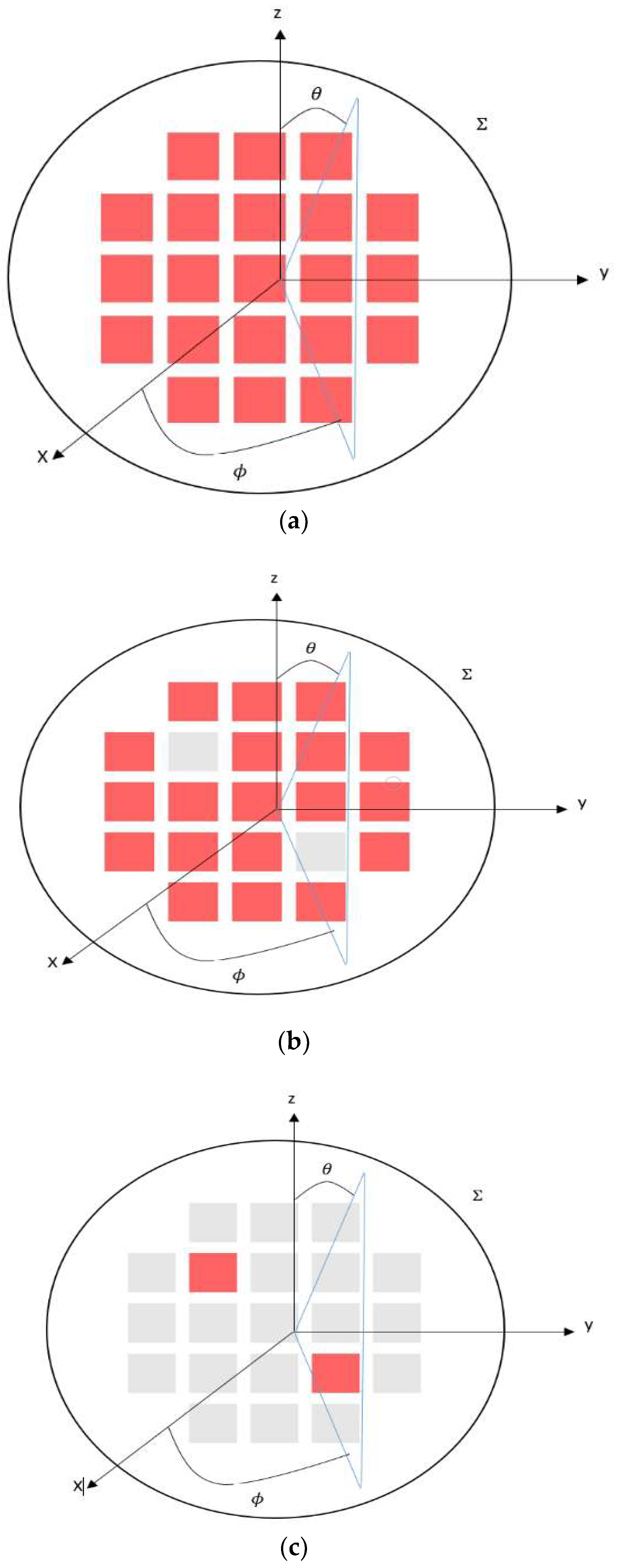
Consider an antenna array in space (Figure 2a). The antenna radiated far-field is usually quantified by phase and amplitude. The AUT is depicted in Figure 2b. All the parameters associated with the AUT are marked with superscript “u”. Specifically, ${\mathit{E}}^u\left(x,y\right)$ is the tangential field situated on the antenna aperture, i.e.,

$${\mathit{E}}^u\left(x,y\right)=E_x^u\left(x,y\right)\widehat{x}+E_y^u\left(x,y\right)\widehat{y},$$

(1)

where $E_x^u\left(x,y\right)\widehat{x}$ and $E_y^u\left(x,y\right)\widehat{y}$ are the x and y planes of the aperture’s electric field, respectively. Far-field $F^u\left(r,\theta ,\varnothing \right)$ is the measured field on part of the hemispherical surface $\left(0\le \theta \le \pi /2,0\le \varphi \le 2\pi \right)$ at radius r from the phase center of the AUT, and $r>2D^2/\lambda$, where D is the diameter. Also, the amplitude and phase of a reference array (RA; array without failures) shown in Figure 2b are assumed to be available. Associated quantities are marked with superscript “o”. ${\mathit{E}}^o\left(x,y\right)$ is the field on the aperture $\mathsf{\Sigma }$ of the reference array (RA) and ${\mathit{F}}^o\left(r,\theta ,\varnothing \right)$ represents the far-field radiation. For the differential antenna (DA) shown in Figure 2c, the tangential distribution $\mathit{E}\left(x,y\right)$ on the aperture $\mathsf{\Sigma }$ is equal to the difference between the field distributions of the reference array and the antenna under test, and the corresponding far-field $\mathit{F}\left(r,\theta ,\varphi \right)$ is expressed as the difference between the fields of reference array (RA) and AUT as

$$\mathit{E}\left(x,y\right)={\mathit{E}}^u\left(x,y\right)-{\mathit{E}}^o\left(x,y\right),$$

(2)

$$\mathit{F}\left(r,\theta ,\varphi \right)={\mathit{F}}^u\left(r,\theta ,\varphi \right)-{\mathit{F}}^o\left(r,\theta ,\varphi \right).$$

(3)

The differential antenna gives a resulting problem in which only the corresponding area to the field modification radiates as a result of failure. By visually monitoring the field distribution on the DA, the identification of faulty elements in the AUT can be observed.

2.1. Number of Far-Field Measurement Points Required

BPA and MMA approaches require a large number of measurement points. In the differential antenna, we assumed the field was localized, i.e., the unknown we wanted to retrieve was very sparse, as shown in Figure 2c. In practice, there are a fewer number of failures than the overall elements N. Sparse recovery algorithms estimate x from a number of measurement points smaller than the number of measurements required by the standard mechanisms. Hence, it is possible to theoretically get a reduction in the number of measurement points. Fuch et al. [20] demonstrated this using total variation (TV), mixed ${\ell }_1/{\ell }_2$ norm, and minimization of ${\ell }_1$. However, better methods/algorithms that require fewer numbers of far-field measurement points for faster array diagnosis are still in demand.

2.2. Signal-to-Noise Ratios (SNRs)

Total variation (TV), mixed ${\ell }_1/{\ell }_2$ norm, and minimization of ${\ell }_1$ techniques are the leading compressive techniques, and they exhibit low efficiency and reliability in antenna diagnosis for low SNRs. This drawback fosters the need for a more robust diagnosis procedure in the presence of noisy data.

3. Compressed Sparse Recovery Methods

The essence of matrix inversion regularization is to initiate a priori facts within the inversion. An adequate approach is needed to get this regularization by approximately reducing the selected norm q of x solution. Then, the optimization to be solved is

$$\underset{\mathrm{x}}{\min }{\Vert X\Vert }_q\mathrm{subject}\mathrm{to}\Vert \mathit{y}-\mathit{A}\mathit{X}{\Vert }_2\le \gamma ,$$

(4)

where $\Vert \ast {\Vert }_q$ represents $l_q$ norm, and $\gamma$ is a function of noise and factors influencing the data. There are various routines available to effectively solve the convex optimization problem of Equation (4) such as References [25,26,27]. The three norms $l_q$, selected based on a priori knowledge of the differential antenna set-up with the diagnosis problem, can now be described for regularization of the inversion. We applied them to conduct diagnosis of both the simulated and measured radiating antennas.

3.1. Total Variation (TV) Norm

Based on a priori knowledge that solution $X$ has small discontinuities as a result of failures present, in addition to the failures, we expect field $X$ to be leveled and almost zero. Hence TV norm is a smooth function to regularize X [27]. Thus, minimizing TV norm is minimizing its gradient, which is the effect of smoothing. Consider a two-dimensional complex dataset $\mathit{X}\in {ℂ}^{M\times N}$; TV norm gives

$$\Vert \mathit{X}{\Vert }_{TV}={\displaystyle \sum }_{m,n}\left|{\mathit{X}}_{m+1,n}-{\mathit{X}}_{m,n}\right|+\left|{\mathit{X}}_{m,n+1}-{\mathit{X}}_{m,n}\right|$$

(5)

$$\Vert vec\left({\mathsf{\nabla }}_x\mathit{X}\right){\Vert }_1+\Vert vec\left(\mathit{X}{\mathsf{\nabla }}_y\right){\Vert }_1.$$

Vec(X) generates vector $N\times M$ which holds the columns of X stacked beneath each other. Gradient matrices ${\mathsf{\nabla }}_x$ and ${\mathsf{\nabla }}_y$ are of $M\times M$ and $N\times N$ size, respectively, which are expressed as

$${\mathsf{\nabla }}_x=\left[\begin{array}{ccc}-1& 1& 0\\ \ddots & \ddots & \\ 0& -1& 1\end{array}\right],\mathrm{and}$$

$${\mathsf{\nabla }}_y=\left[\begin{array}{ccc}-1& & 0\\ 1& \ddots & \\ & \ddots & -1\\ 0& & 1\end{array}\right].$$

Then, the optimization problem in Equation (4) transforms to

$$\underset{\mathit{X}}{\min }\Vert \mathit{X}{\Vert }_{TV}\mathrm{subjects}\mathrm{to}\Vert \mathit{y}-\mathit{A}vec{\left(\mathit{X}\right)\Vert }_2\le ϵ.$$

(6)

3.2. The ${\ell }_1$ Norm

Since there is a sparse solution $X$; then, a space of search could be drastically reduced by the introduction of a priori knowledge in inversion. Specifically, the ${\ell }_1$-norm ($\Vert X{\Vert }_1={{\displaystyle \sum }}_k\left|x_k\right|)$ is the leading convex surrogate of an acceptable estimate sparsity of the vector (quasi-norm ${\ell }_0$ that calculates nonzero occurrences of a given vector). As a result, ${\ell }_1$ norm is an efficient approach to enhance sparse solutions [2,5,10,19]. The regularization problem is then

$$\underset{X}{\min }\Vert X{\Vert }_1\mathrm{subject}\mathrm{to}\Vert \mathit{y}-\mathit{A}X{\Vert }_2\le ϵ.$$

(7)

Minimizing ${\ell }_1$-norm imposes the pointwise sparsity of solution per sample $x_k$ of the field on the aperture of the DA.

3.3. Mixed ${\ell }_1/{\ell }_2$ Norm

The radiating aperture’s position and dimensions can also be taken. The solution X is grouped into G groups $X^g$, which corresponds to the individual radiating element’s aperture g. For a faulty element, all regions of discretization $x_k^g$ in the aperture will be faulty (nonzero). Let vector X of dimension $M\times N$ be divided into G non-overlapping groups depicted $X^g$ of size $N_g$, such as ${{\displaystyle \sum }}_{g=1}^G{N}_g=MN.$ Hence, the mixed ${\ell }_1/{\ell }_2$ norm is given as

$$\Vert X{\Vert }_{1,2}={\displaystyle \sum }_{g=1}^G\Vert X^g{\Vert }_2={\displaystyle \sum }_{g=1}^G\sqrt{{\left|x_1^g\right|}^2+\dots +{\left|x_{N_g}^g\right|}^2}.$$

(8)

The mixed ${\ell }_1/{\ell }_2$ norm has similar behavior to ${\ell }_1$ norm on vector $\Vert X^1{\Vert }_2$, …, $\Vert X^g{\Vert }_2$, …, $\Vert X^G{\Vert }_2$; it, therefore, induces group sparsity at the radiating aperture level. The regularized inversion problem is then expressed as

$$\underset{X}{\min }\Vert \mathit{X}{\Vert }_{1,2}\mathrm{subject}\mathrm{to}\Vert \mathit{y}-\mathit{A}\mathit{X}{\Vert }_2\le ϵ.$$

(9)

4. Resolution via Bayesian Compressive Sensing

For a planar antenna configuration of N elements positioned at coordinates $\left(x_n{y}_n\right)$, n = 1, …, N, with error-free excitations ${\alpha }_n$, n = 1, …, N, beaming a familiar field $E\left(u,v\right),\left(whereu=sin\theta cos\phi andv=sin\theta sin\phi \right)$, referencing a noisy case with element failure, the estimated far-field radiation pattern of (AUT) is expressed as

$$\tilde{E}\left(u_l,v_l\right)={\displaystyle \sum }_{n=1}^N{\beta }_n{e}^{j\frac{2\pi }{\lambda }\left(x_n{u}_l+y_n{v}_l\right)}+v_l,$$

(10)

where $\left(u_l,v_l\right)$ for l = 1, …, L is the angular location of the l-th angular sample, and $v_l$ is the noise effect considered as Gaussian-distributed with zero mean and variance ${\sigma }^2$. ${\beta }_n$, n = 1, …, N, is the failed excitations vector, expressed as

$${\beta }_n=\{\begin{array}{l}h{\alpha }_{n}withprobability\mathsf{\Phi }\\ {\alpha }_{n}otherwise\end{array},n=1,\dots ,N.$$

(11)

$h\in \left(0,1\right)$ is the failure factor, while $\mathsf{\Phi }$ is the rate of failure, and ${\alpha }_n$ is the weighting coefficient. From knowledge of the difference in field pattern, $W\left(u_l,v_l\right)=E\left(u_l,v_l\right)-\tilde{E}\left(u_l,v_l\right),l=1,\dots ,L$, array failures can be estimated by determining the minimum ${\ell }_0-norm$ vector

$$\underset{\_}{\mathsf{{\rm Y}}}=\{{\mathsf{{\rm Y}}}_n={\alpha }_n-{\beta }_n;n=1,\dots ,N\},$$

(12)

which satisfies

$$\underset{\_}{W}-\underset{\_}{\underset{\_}{\mathsf{\Psi }}}\underset{}{\mathsf{{\rm Y}}}=\underset{\_}{v}.$$

(13)

The aim is to determine the entries of the “failure” vector $\underset{\_}{W}=\{W\left(u_l,v_l\right);l=1,\dots ,L\},\underset{\_}{v}=\{v_l;l=1,\dots ,L\}$ from the prior knowledge of the difference between the field samples in Equation (10) on the AUT and those of the golden antenna with coefficients ${\alpha }_n$ n = 1$,\dots ,N$. Against the deterministic approaches aimed at retrieving the vector $\underset{\_}{\gamma }$ with minimum ${\ell }_0-norm$ satisfying the condition of Equation (13), $\underset{\_}{\underset{\_}{\mathsf{\Psi }}}$ is the $L\times N$ radiation measurement matrix expressed as

$$\underset{\_}{\underset{\_}{\mathsf{\Psi }}}=\left[\begin{array}{ccc}{e}^{\left[j2\pi \left(x_1{u}_1+y_1{v}_1\right)\right]}& \dots & e^{\left[j2\pi \left(x_N{u}_1+y_N{v}_1\right)\right]}\\ ⋮& \ddots & ⋮\\ e^{\left[j2\pi \left(x_1{u}_L+y_1{v}_L\right)\right]}& \dots & e^{\left[j2\pi \left(x_N{u}_L+y_N{v}_L\right)\right]}\end{array}\right].$$

(14)

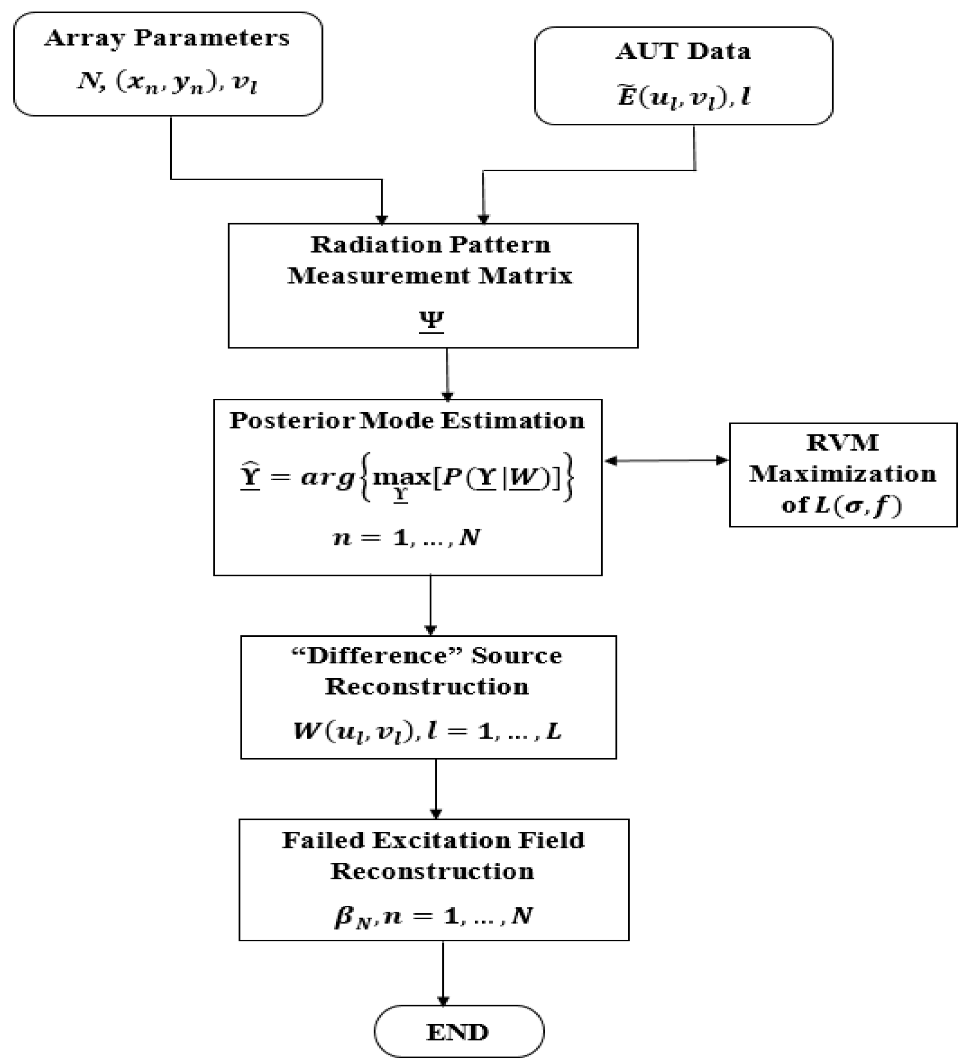
Hence, the BCS technique (summarized in Figure 2) can be employed to determine the sparsest solution $\underset{\_}{\widehat{\mathsf{{\rm Y}}}}$ to the problem

$$\underset{\_}{\widehat{\mathsf{{\rm Y}}}}=arg\left\{\underset{\underset{\_}{\mathsf{{\rm Y}}}}{\max }[P(\underset{\_}{\mathsf{{\rm Y}}}|\underset{\_}{W})]\right\},$$

(15)

which gives

$$\underset{\_}{\widehat{\mathsf{{\rm Y}}}}=\frac{1}{{\sigma }_{NP}}\left[\frac{\underset{\_}{\underset{\_}{{\mathsf{\Psi }}^T}}\underset{\_}{\underset{\_}{\mathsf{\Psi }}}}{{\sigma }_{NP}}+diag\left({\underset{\_}{f}}_{NP}\right)\right],$$

(16)

where T is the transpose operator, and ${\sigma }_{NP}$ and ${\underset{\_}{f}}_{NP}$ are the figures that are used to maximize the likelihood function

$$L\left(\sigma ,\underset{\_}{f}\right)=-\frac{1}{2}\left[Nlog2\pi +log\left|\underset{\_}{\underset{\_}{C}}\right|+\underset{\_}{W^T}\underset{\_}{\underset{\_}{C^{-1}}}\underset{\_}{W}\right].$$

(17)

Equation (11) is computed using RVM [29], with $\underset{\_}{\underset{\_}{C}}=\sigma +\underset{\_}{\underset{\_}{\mathsf{\Psi }}}\underset{\_}{\underset{\_}{F^{-1}}}\underset{\_}{\underset{\_}{{\mathsf{\Psi }}^T}}$, where $\underset{\_}{\underset{\_}{F}}=diag(\underset{\_}{f})$.

The implementation of the BCS technique (as shown in Figure 3) is summarized in Algorithm 1.

Algorithm 1. Proposed diagnostic procedure

a.  Step 1—Array parameter selection and definition of problem: For each element ($\mathit{n}=\mathbf{1},\dots \mathit{N}$), accumulate the array field at N measurement points (reference antenna) and randomly sample the AUT field. Appropriate the noise variance and threshold for the maximization of $\mathit{L}\left(\mathit{\sigma },\underset{\_}{\mathit{f}}\right)$. b.  Step 2—Radiation pattern measurement matrix $\underset{\_}{\underset{\_}{\mathit{\Psi }}}$ definition. Input the parameters of $\underset{\_}{\underset{\_}{\mathsf{\Psi }}}$. c.  Step 3—Posterior mode estimation. Maximize Equation (10) iteratively to estimate $\mathit{\sigma }\mathit{a}\mathit{n}\mathit{d}\underset{\_}{\mathit{f}}$ using the RVM procedure [29]. d.  Step 4—Source difference reconstruction. Determine $\mathit{W}\left({\mathit{u}}_{\mathit{l}},{\mathit{v}}_{\mathit{l}}\right)$ for l = 1, …, L. e.  Step 5—Failed field excitation reconstruction. Determine the vector of failed excitations ${\mathit{\beta }}_{\mathit{n}}\left(\mathit{n}=\mathbf{1},\dots ,\mathit{N}\right)$ using Equation (11).

5. Simulations and Analysis

Assessing the performance of the BCS algorithm, we consider an RA with N = 316 with Taylor taper and peak sidelobe level of −25 dB. Assuming a complete failure (h = 0), the given percentage of failed elements is $\mathsf{\Phi }=4\%$. To determine the detection error numerically, the index of detection can be expressed as

$$\zeta =100\times \frac{{{\displaystyle \sum }}_{n=1}^N{\left|{\mathsf{{\rm Y}}}_n-{\widehat{\mathsf{{\rm Y}}}}_n\right|}^2}{{{\displaystyle \sum }}_{n=1}^N{\left|{\mathsf{{\rm Y}}}_n\right|}^2},$$

(18)

where ${\mathsf{{\rm Y}}}_n$ and ${\widehat{\mathsf{{\rm Y}}}}_n$, n = 1, …, N, are the real and predicted failure entries of vector $\underset{\_}{\mathsf{{\rm Y}}}$. The uniformly sampled (k = 316 samples) far-field radiation pattern is within (u, v) space, with the signal-to-noise ratio SNR = 30 dB. 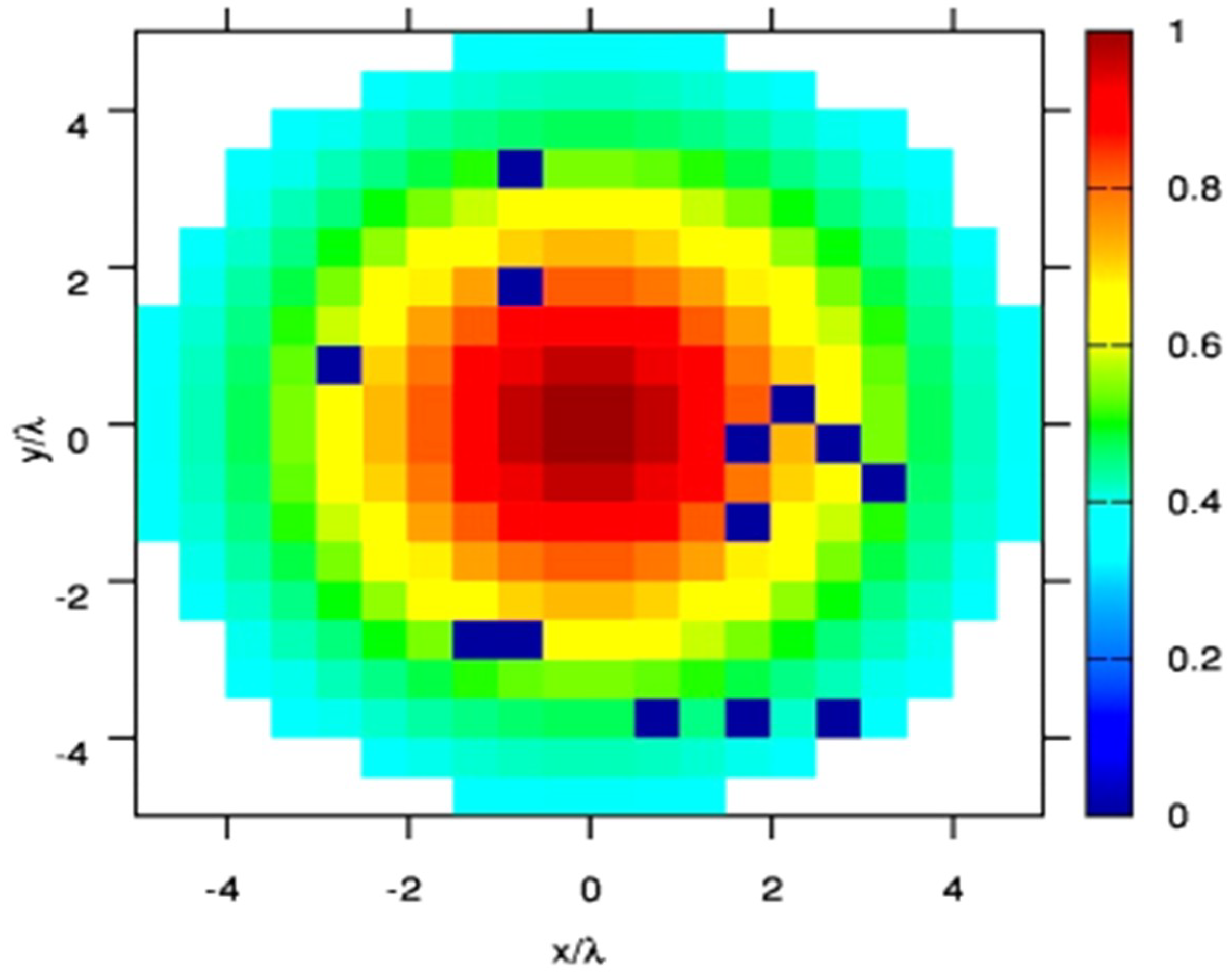The configuration of the AUT is presented in Figure 4, while the excitation coefficients ${\beta }_n$ of the failed array are equally shown. 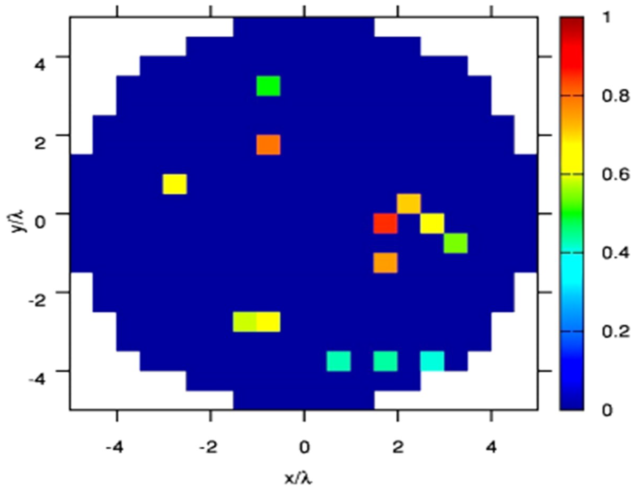Figure 5 shows ${\widehat{\mathsf{{\rm Y}}}}_n$ of the failure vector estimated via the proposed technique. As expected, there is good correlation between the location and the number of the real and predicted failed elements. Accuracy of the estimation was ascertained by a very small index of detection figure of $\zeta =3.83\times {10}^{-3}$.

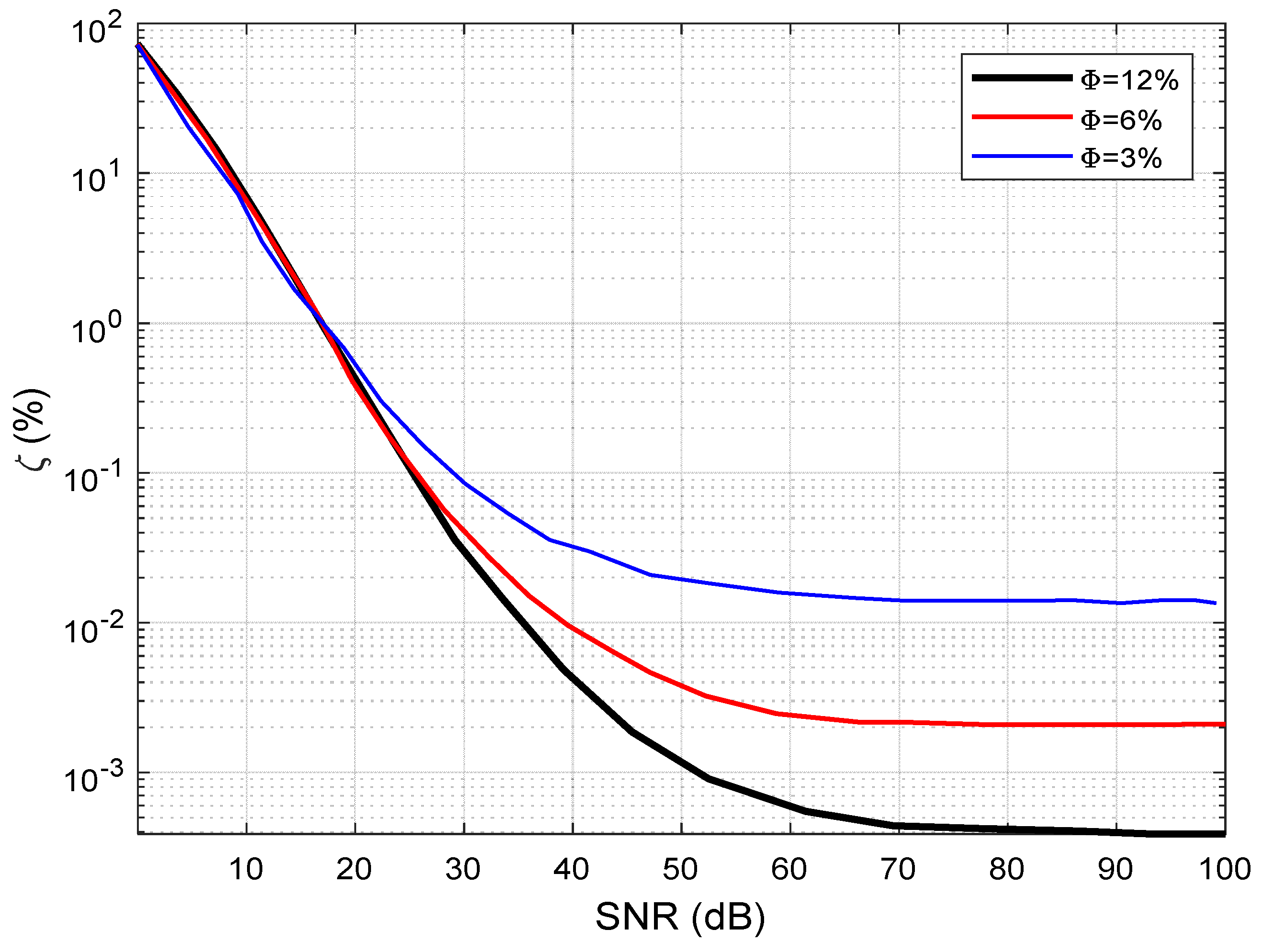
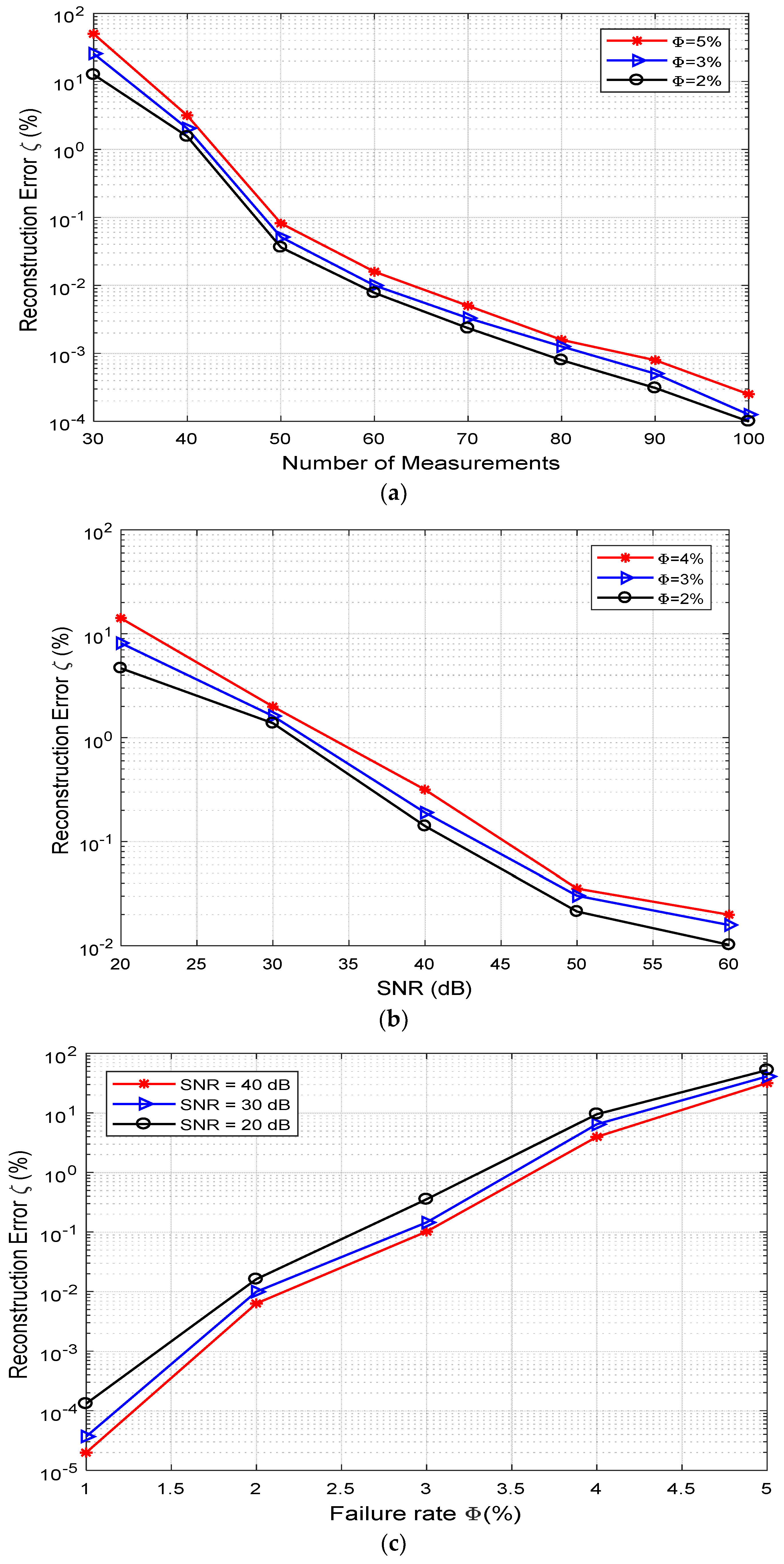
To analyze the impact on performance metrics of the technique of the noise on far-field patterns, we ranged the SNR between 0 dB and 100 dB. Figure 6 shows the obtained result. The estimation error $\zeta$ is high for low SNRs irrespective of failed element percentage. Also, for higher SNR, the robustness of the approach increases, which shows that the best performances are attained at $\mathsf{\Phi }=3\%$. 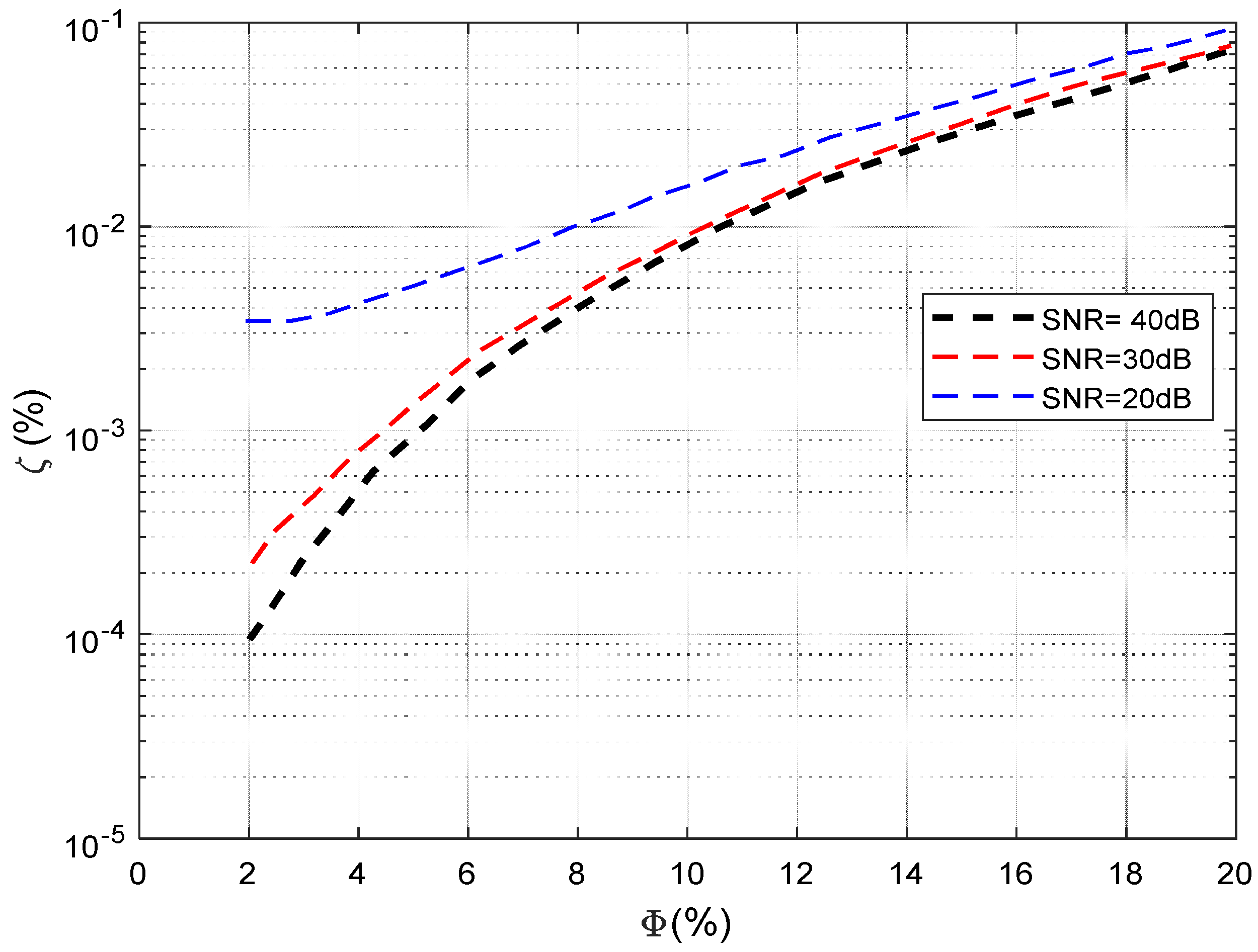The impact of the percentage of failed elements on the performance of the method proposed was also assessed by varying the percentage of the failed elements from $\mathsf{\Phi }=2\%$ to $\mathsf{\Phi }=20\%$ (see Figure 7). Expectedly, the performance metrics of the approach reduced for a higher percentage of failed elements, even for very low noise levels. Conversely, the approach achieved a degree acceptable accuracy until about $10\%$ of damaged elements at any SNR. This result validates the efficiency of the BCS technique in the diagnosis of sparse failures in arrays.

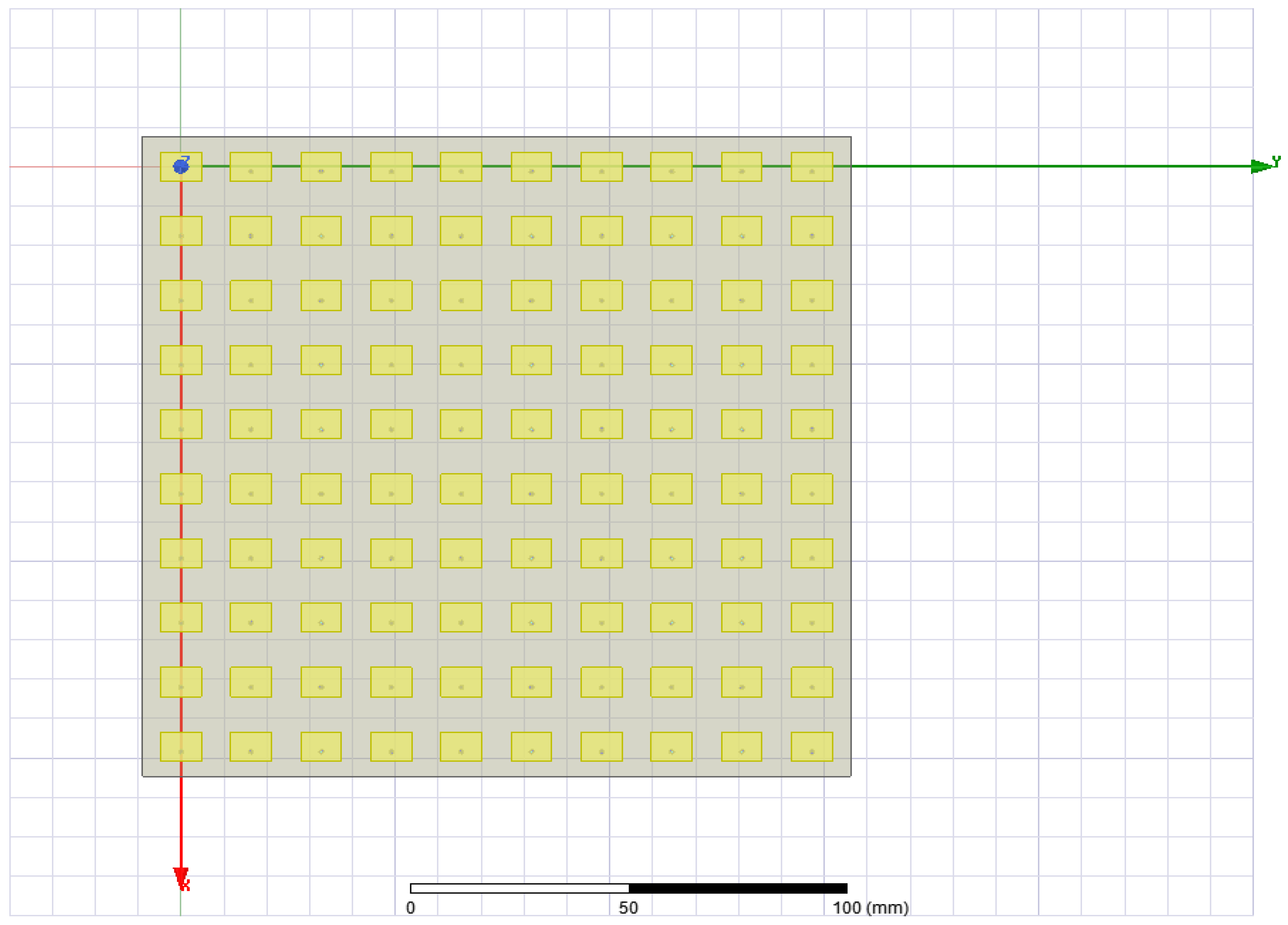
Example Using Full-Wave Simulation Set-Up

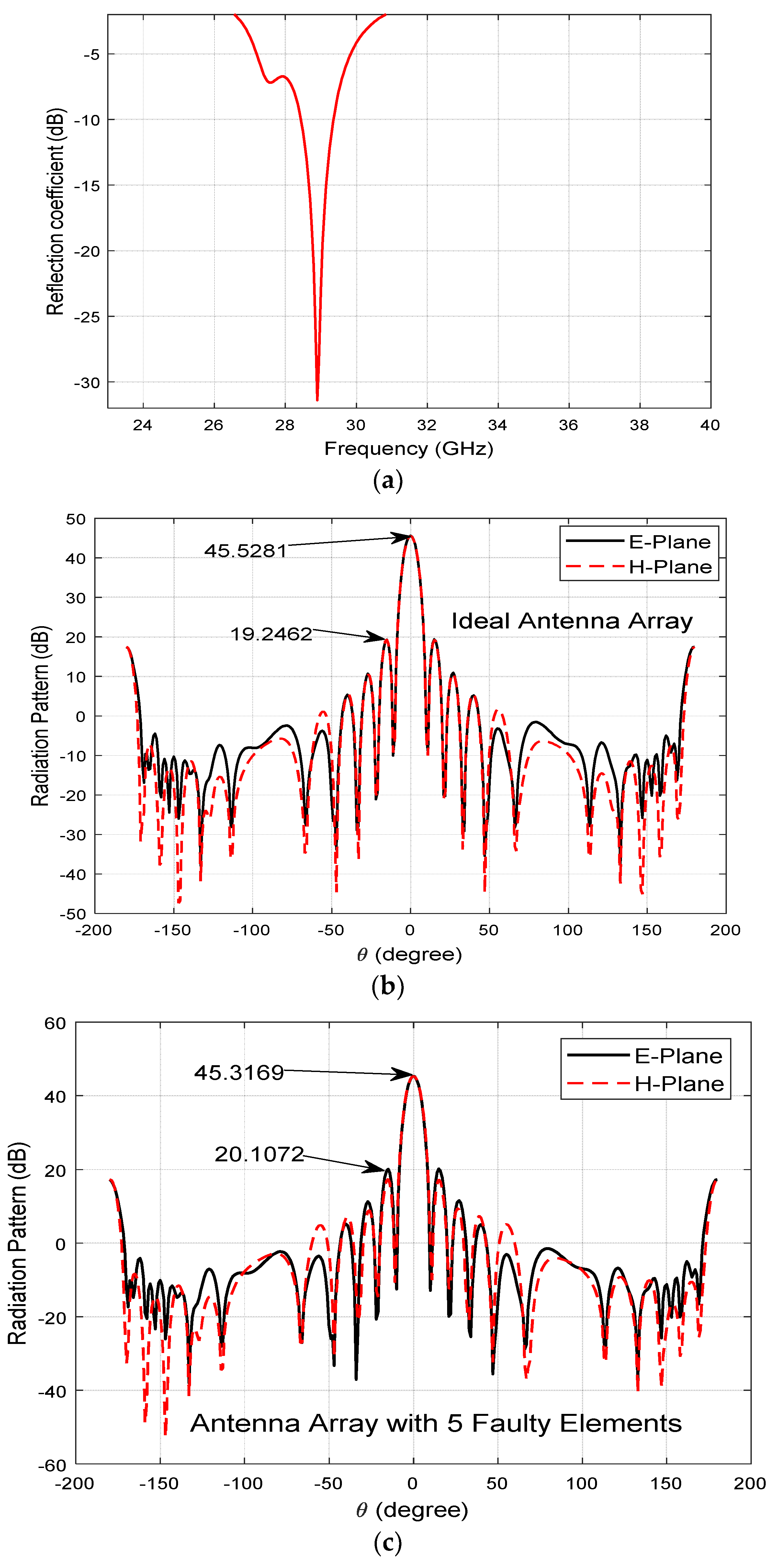
A $10\times 10$ microstrip patch antenna array with an aperture size of 31 × 31 mm² operating at 28.9 GHz was designed, as shown in Figure 8. We designed and computed the radiation pattern and S-parameter (Figure 9) of the antenna using full-wave three-dimensional (3D) EM software Ansys HFSS v. 17. The elements were uniformly spaced along the x and y directions. Each element had an excitation port. Practically, measurements are made impure by noise; hence, a Gaussian noise n was added to the data on both radiation patterns as ${\mathit{y}}_n^q={\mathit{y}}^q+{\mathit{n}}^q$, with $q=\left\{r,d\right\}$. The noise level was determined by signal-to-noise ratio (SNR) defined from the maximum received field magnitude fitting the dynamic measurement range. The noise was estimated as

$$n^q=\frac{\mathcal{N}\left(0,1\right)+j\mathcal{N}\left(0,1\right)}{\sqrt{2}}max\left|{\mathit{y}}^q\right|\times {10}^{-SN{R}_{dB}/20},$$

(19)

where $\mathcal{N}\left(0,1\right)$ is a Gaussian random vector of mean 0 and standard deviation 1.

The faulty elements cause low gain, high sidelobe level, wider beamwidth, lower front-to-back ratio, and a boresight pointing error. The effects are shown in Figure 9b. A Rogers 5880 dielectric substrate with 20 mm thickness and 3.48 dielectric constant was used for the antenna design because it has low signal loss, low dielectric loss, low outgassing (which is good for space applications), and cheap circuit fabrication. The total number of elements in the array was 100. The length and width of a single patch were estimated to be 7.4 mm and 9.5 mm, respectively. Elements were uniformly spaced by 8.947 mm and 6.847 mm along x and y, respectively.

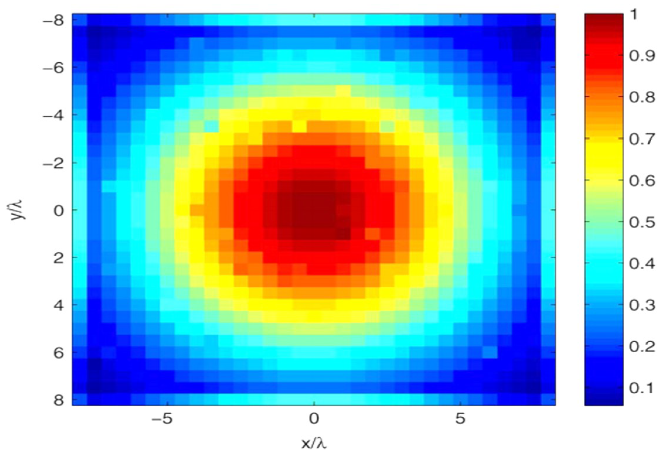
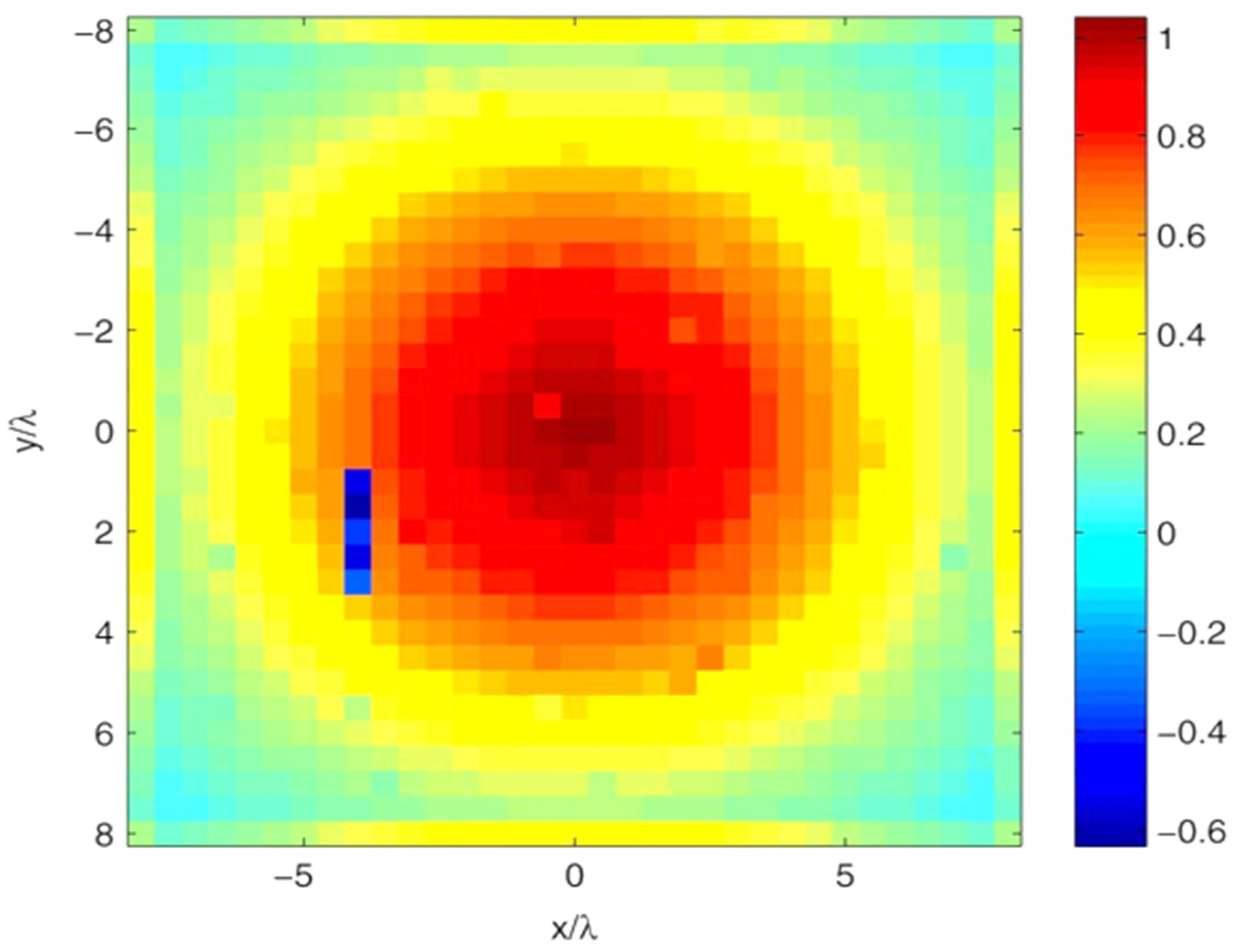
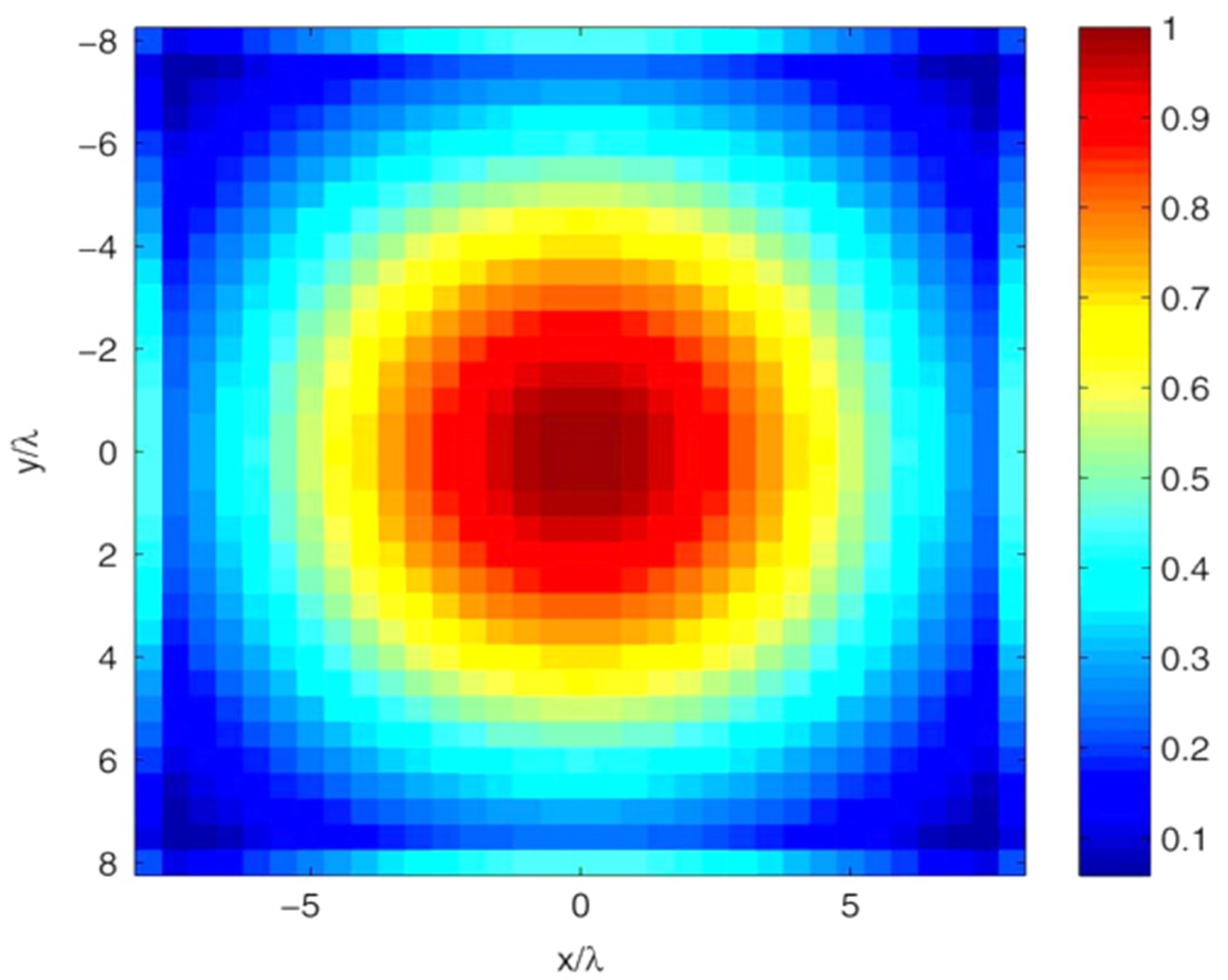
All elements were fed with the same excitation value which equal to one to emulate the array without failure (reference array). Then K failures (in this case, the estimated percentage of failure rate) were also initiated intentionally by making the excitation equal to zero in order to model the AUT effectively. At first, we considered the reference array, i.e., the array without failures. 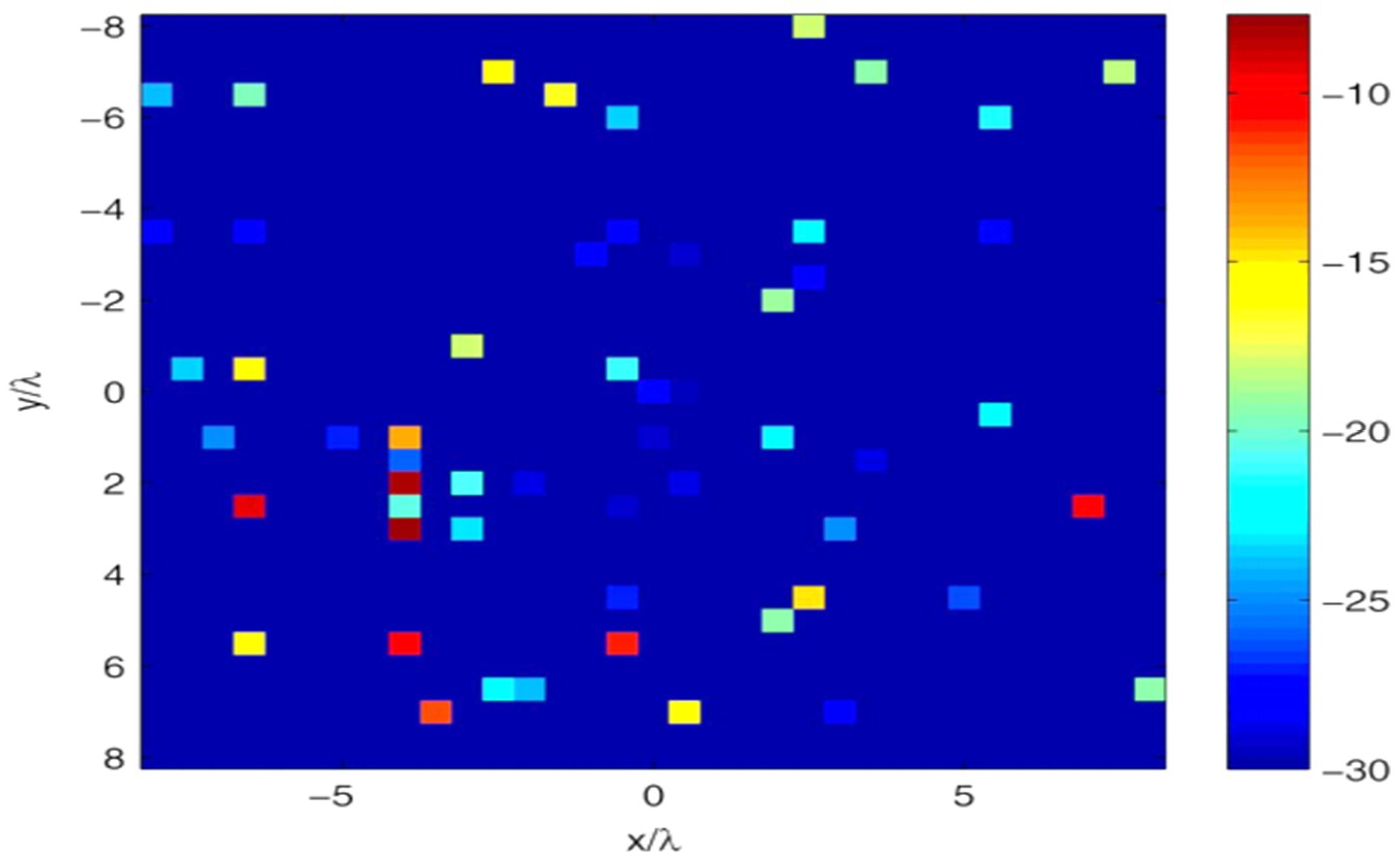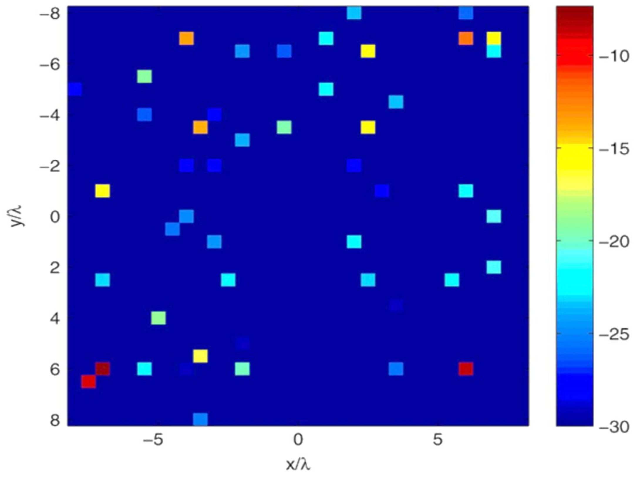The excitation coefficients are depicted in Figure 10, and the reconstructed excitation coefficients are presented in Figure 11. Also, for quantitative knowledge of the error estimated, the computed excitation error in dB is shown in Figure 12. The result indicates an exact reconstruction in the case of the reference array, and shows a low probability of a false alarm.

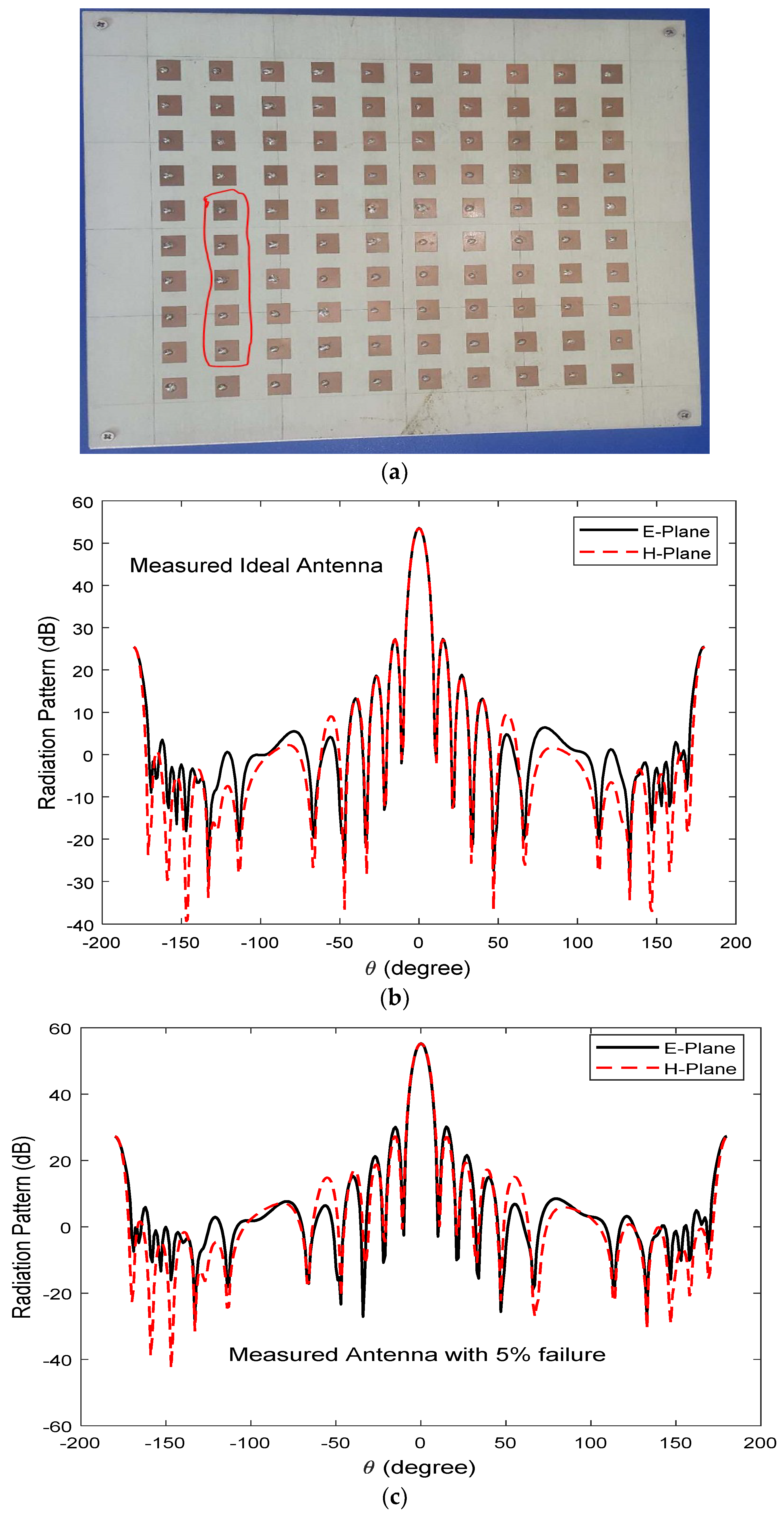
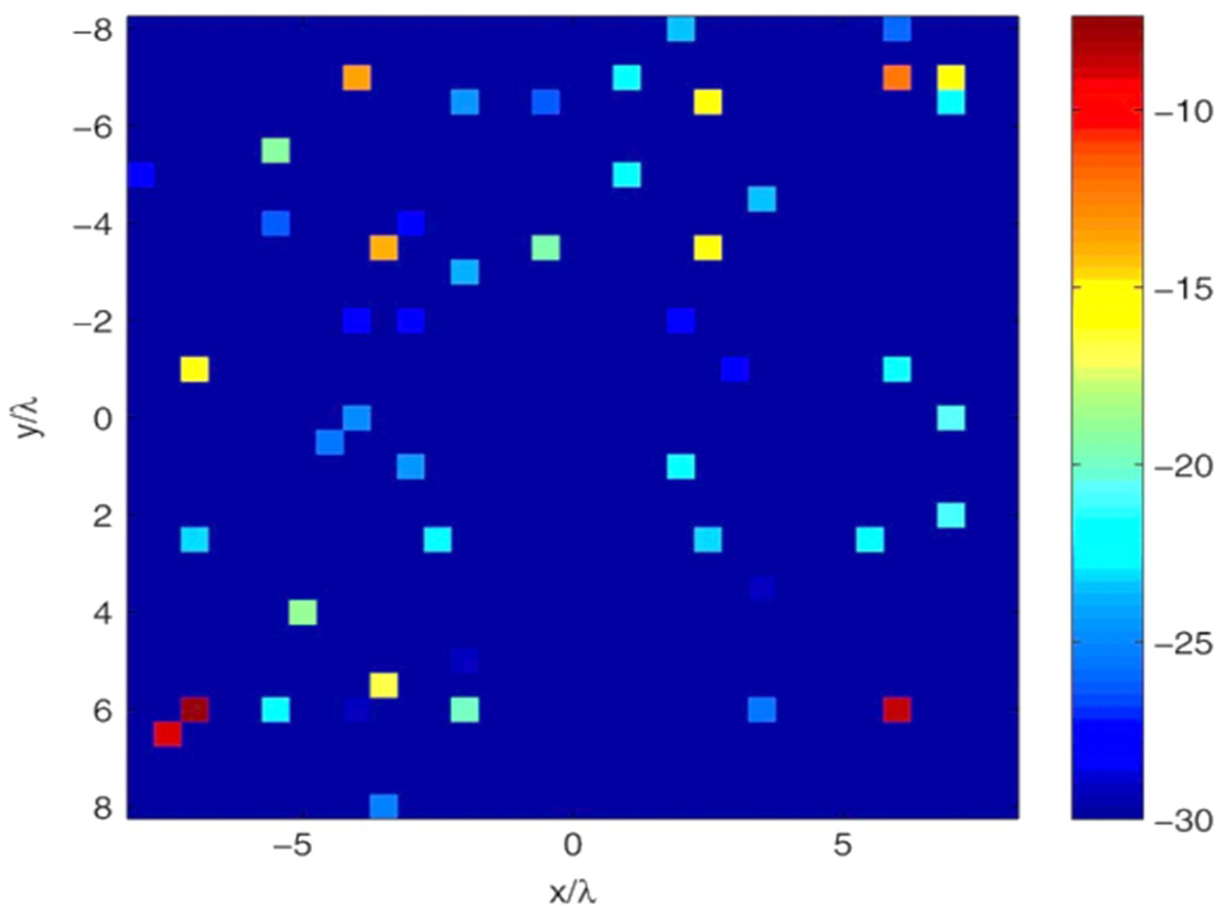
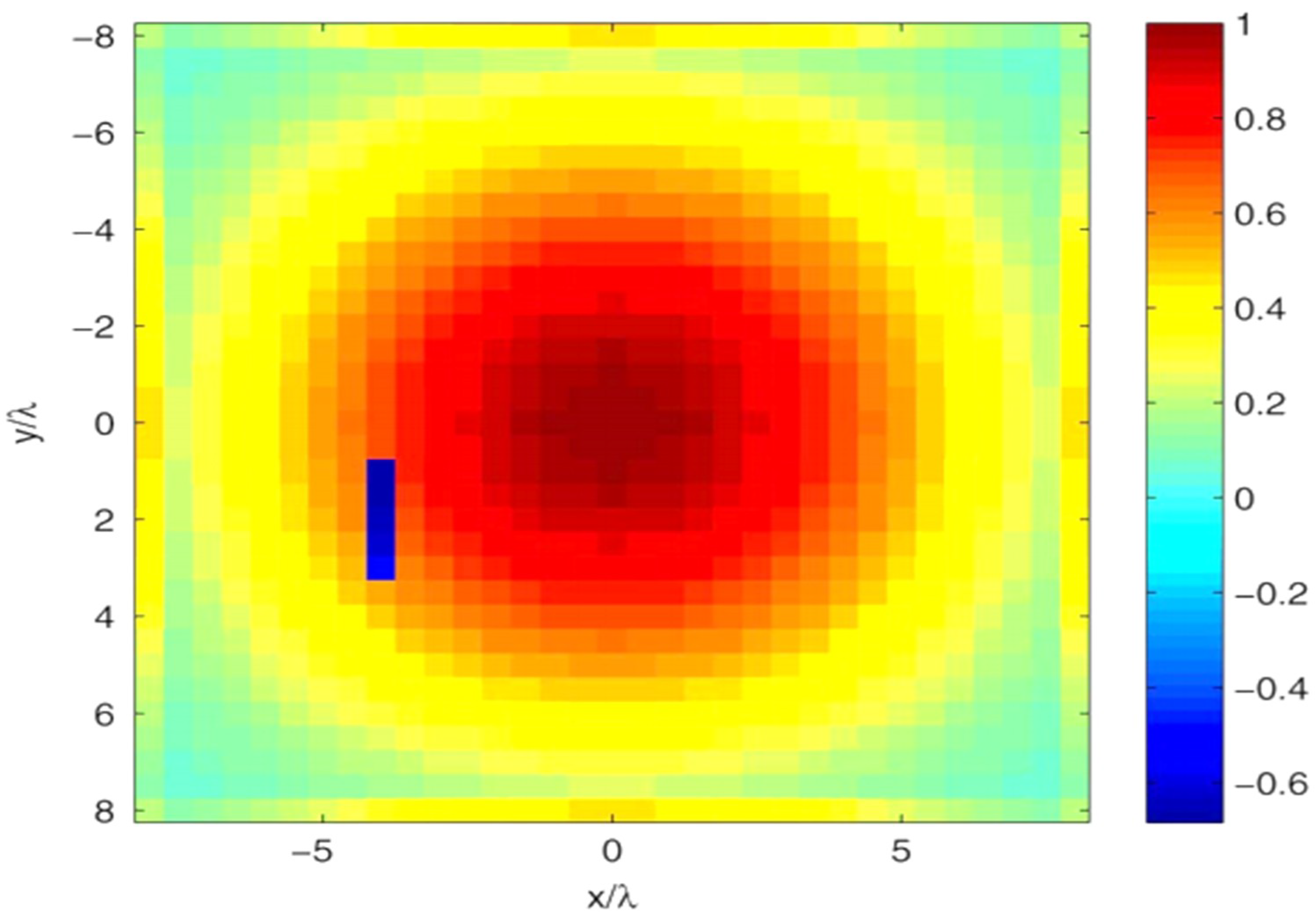
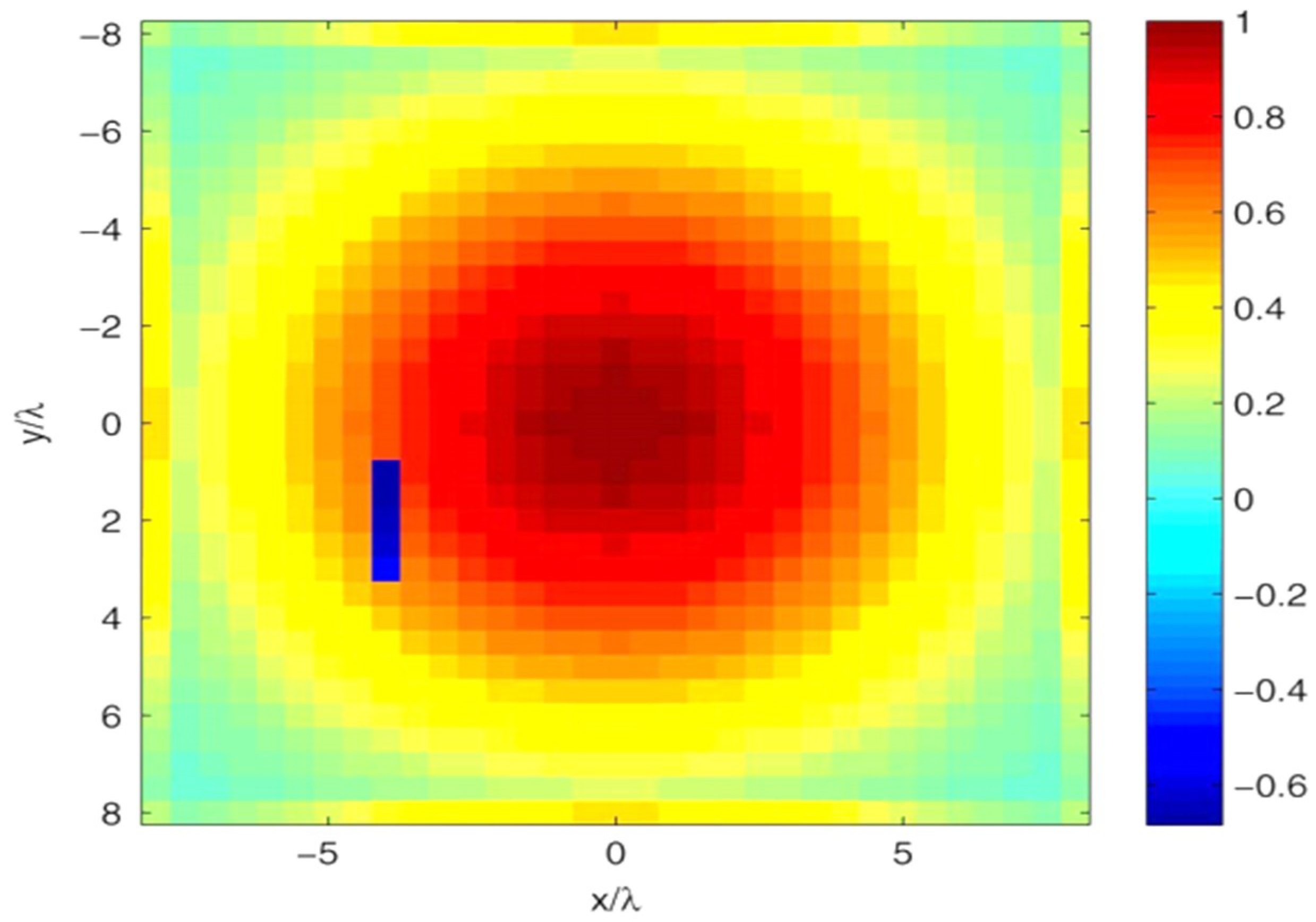
Also, considering an AUT with K = 5 element failures ($\mathsf{\Phi }=5\%$) (elements with zero excitation) because failed elements are usually of small number in practice, the resulted excitation coefficients are presented in Figure 13, and the estimated excitations by 30 random noisy measurement points are presented in Figure 14, while the dB excitation error is depicted in Figure 15. The result is an indication of good estimation of RA excitations and the locations of the faulty elements.

6. Antenna Array Diagnosis from Measured Data

6.1. Measurement Set-Up

The proposed diagnostic technique was subjected to an experimental test, as presented in Figure 16. Although, this was a controlled environment (anechoic chamber), a more practical condition (uncontrolled environment) was also possible using the same set-up in Figure 16, without the chamber. The AUT was a $10\times 10$ microstrip patch antenna array (see Figure 17a), reradiating a signal tilted in the two planes. Figure 17b,c show the measured radiation patterns for an ideal antenna and defected antenna, respectively. It can be see that the failure causes higher sidelobe level, reduced gain, lower front-to-back ratio (FBR), wider beamwidth, and a boresight pointing error.

The antenna was particularly designed and fabricated for this purpose, and each element had its feeding port which was excited using a power divider. Five radiating elements in the array were not excited (zero excitation) to successfully emulate the failure of elements. The AUT set-up is depicted in Figure 18. About 1000 co-polar and cross-polar measurements were taken on the far-field half-sphere at 28.9 GHz in an anechoic chamber (see Figure 18).

Radiation pattern measurements obtained from the array with five faulty elements were fed into the proposed algorithm for post-processing. The reconstructed excitation error which identified the specific faulty elements is depicted in Figure 19, and the corresponding dB equivalence is shown in Figure 20. Moreover, the performance metrics of the BCS-based approach were experimentally tested, and are shown in Figure 21. Figure 21a shows the obtained reconstruction error versus the measurement number at different degrees of failure. The error decreased as the number of measurement points increased irrespective of failure percentage. The reconstruction error profile increased with increased failure rate. In Figure 21b, it is demonstrated how the reconstruction error profile changes with SNR for different failure rates. The reconstruction error degraded exponentially with increased SNR independent of failure rate. The reconstruction error increased with increased failure rate. Figure 21c depicts reconstruction error versus different levels of failure for various SNRs. It can be observed that the error increased with increased failure rate. Also, the reconstruction error decreased as SNR increased.

The imperfection of the curves (compared to the simulation) could be attributed to measurement errors, and errors due to experimental set-ups which provide different conditions from those in the simulations. The experiment was conducted in an anechoic chamber, which is a controlled environment. Hence, the results presented here may show a little variation if the experiment is conducted in a more practical environment (i.e., uncontrolled environment). Moreover, the BCS-based procedure presented here can be trusted to effectively and reliably address sparse recovery problems, particularly the detection of faulty radiators in planar arrays for next-generation 5G wireless communications. Once the suitable data are collected, and used to diagnose the array, then the array feeding network can be recalibrated to restore the needed radiation features via excitation reconfiguration of the healthy antenna elements. However, prior knowledge of the golden array must be provided, and the failure rate is relatively smaller than the array size. Therefore, from the simulation results verified by the experiment, the BCS-based approach is adequate and reliable for noisy data. This technique overcomes the shortcomings of BPA, MMA, etc., demanding off-line phase training to form accurate mapping between the response of the AUT and the failure location. Hence, the proposed procedure will be highly useful for millimeter-wave planar array optimal performance.

6.2. Antenna Array Diagnosis from Simulated and Measured Far-Field Radiation Patterns

There are differences between the simulated and measured antenna patterns due to measurements errors, uncontrollable array fabrication errors, and experimental set-ups that give different conditions from the simulations. For example, in our design, a finite flange was employed to feed the ground plane. Hence, the induced current on flange rescattered and redistributed somehow against the very large ground plane which was used for the simulations. Antenna array diagnosis procedures based on simulated radiation pattern (such as References [3,16,17,18,27,35]) may not be reliable and accurate, except when tested with the corresponding measured data. Although, in this work, simulation and measurement data exhibit little difference in field intensity of the identified faulty elements (in Figure 14 and Figure 19, respectively) caused by the electromechanical coupling effect. In general, the proposed BCS-based approach shows good reliability and accuracy against both simulated and measured far-field radiation patterns.

6.3. Number of Measurement Points versus Noisy Measured Data

Measurement points affect field reconstruction fidelity and, hence, the scheme of diagnosis. The proposed BCS-based procedure performed well despite significantly reduced measurement data due to added sparse information. According to the study and experiments performed by Fuch et al. [14], total variation (TV), mixed ${\ell }_1/{\ell }_2$ norm, and minimization of ${\ell }_1$ techniques require 64 measurement points for accurate reconstruction and diagnostics, compared to the BCS technique that requires 30 or less measurement points. The proposed method significantly reduces the number of measurements needed for diagnosis as compared to those three approaches. Since the speed of diagnosis is inversely related to the required number of measurement points, the BCS approach enables a faster diagnosis of antenna arrays.

Also, according to the diagnostic procedures proposed by Fuch et al. [14], total variation (TV), mixed ${\ell }_1/{\ell }_2$ norm, and minimization of ${\ell }_1$ techniques can only accommodate measured data with the lowest SNR of 40 dB. A lower SNR results in bad diagnostics for the three procedures. However, there are practical measurements that exhibit SNRs lower than 40 dB which require diagnosis. To this advantage, the proposed BCS approach was theoretically and practically used to diagnose antenna arrays from measurement data with 20 dB SNR. It can equally adapt to measured data with lower SNR. The comparison is summarized in

Table 1. Comparison between Bayesian compressive sensing (BCS)-based approach and previous compressive sensing techniques. SNR—signal-to-noise ratio.

Approach	This Work (BCS-Based)	Minimization of ${\mathit{\ell }}_1$ [14,36]	Total Variation (TV) [14,37]	Mixed ${\mathit{\ell }}_1/{\mathit{\ell }}_2$ Norm [14,38]
Required signal characteristics	Amplitude	Amplitude or Phase	Amplitude or Phase	Amplitude or Phase
Minimum SNR (dB)	$20$	$40$	$40$	$40$
Nature	More complex	Simpler	Simple	Complex
Required measurement points	30	64	64	64
Post-processing time (s)	7.6	0.4	2.0	4.9

. The BCS approach requires a few seconds more computational time; however, this is very small with respect to the measurement time cost. Therefore, the proposed method shows its robustness to noisy measured data, and a reliable diagnosis was obtained for low SNRs.

7. Conclusions

A faster and robust antenna array diagnosis procedure from far-field radiation pattern measurement points using Bayesian compressive sensing (BCS) approach was proposed in this paper. Previous compressive sensing procedures exhibit shortcomings based on reliability with noisy data, and require a large number of far-field measurement points. The proposed method solves these problems by formulating planar array diagnosis within the concept of the BCS framework, resolved using fast relevance machine (RVM). We are not the first to apply the BCS approach to antenna array diagnosis. It was applied only to linear configurations in References [15,16] without practical measurements, which are fundamental for testing any procedure. To the best knowledge of the authors, this is the first attempt to apply the BCS approach to planar antenna array diagnosis from far-field measurement points, validated with experimental measurements. Diagnoses from simulated and measured far-field points from a designed microstrip patch antenna array show the method’s robustness to additive data noise, as well as its reconstruction accuracy and faster diagnosis speed, which is desired in practical applications. Hence, the proposed method is a better practical choice whenever an efficient, faster, and more reliable antenna array diagnosis (testing) is needed.

Also, it is important to comment on the choice of sampling strategy. We considered a random selection of measurement points from a uniform lattice. The choice of the sampling technique is not critical because it affects all the techniques in the same manner at the far-field. However, it was pointed out, from a non-uniform near-field lattice, that proper non-uniform random sampling (NURS) using a priori information on the problem provides meaningful reduction in the cardinality of the set of measured data compared to uniform random sampling and random sampling from a λ/2 equispaced dataset [39]. Moreover, the BCS-based technique was compared to other methods using the data reported in the literature. In the future, we will compare different techniques using experimental data from controlled and uncontrolled environments, and the same parameters in order to quantify the error affecting the result of different techniques. For example, we will determine what happens if we use 30 measurements instead of 64 measurements in the experimental data using ${\ell }_1$ minimization, i.e., the same number of data used by the BCS, as well as the error compared to BCS. A complete comparison among the techniques using real data is still absent in the present literature.

References

1. Oliveri, G.; Donelli, M.; Massa, A. Linear array thinning exploiting almost difference sets. IEEE Trans. Antennas Propag. 2009, 57, 3800–3812. [Google Scholar] [CrossRef]
2. Oliveri, G.; Manica, L.; Massa, A. ADS-based guidelines for thinned planar arrays. IEEE Trans. Antennas Propag. 2010, 58, 1935–1948. [Google Scholar] [CrossRef]
3. Carlin, M.; Oliveri, G.; Massa, A. On the robustness to element failures of linear ADS-thinned arrays. IEEE Trans. Antennas Propag. 2011, 59, 4849–4853. [Google Scholar] [CrossRef]
4. 5G Vision White Paper, DMC R&D Center. Samsung Electronics Co., Ltd., 2015. Available online: http://www.samsung.com/global/business-images/insights/2015/Samsung-5G-Vision-0.pdf (accessed on 4 October 2018).
5. 5G: A Technological Vision, HUAWEI white Paper. Huawei Technologies Co.: Shenzhen. Available online: http://www.huawei.com/5gwhitepaper/ (accessed on 4 October 2018).
6. Frenzel, L. Ka-Band Transceiver Implements MIMO and Beamforming for 5G. Available online: Electronicdesign.com (accessed on 8 October 2018).
7. Lee, J.J.; Ferrer, E.M.; Woollen, D.P.; Lee, K.M. Near-field probe used as a diagnostic tool to locate defective elements in an array antenna. IEEE Trans. Antennas Propag. 1988, 36, 884–889. [Google Scholar] [CrossRef]
8. Gattoufi, L.; Picard, D.; Samii, Y.R.; Bolomey, J.C. Matrix method for near-field diagnostic techniques of phased array antennas. In Proceedings of the IEEE International Symposium on Phased Array Systems and Technology, Boston, MA, USA, 15–18 October 1996; pp. 52–57. [Google Scholar]
9. Bucci, O.M.; Migliore, M.D.; Panariello, G.; Sgambato, G. Accurate diagnosis of conformal arrays from near-field data using the matrix method. IEEE Trans. Antennas Propag. 2005, 53, 1114–1120. [Google Scholar] [CrossRef]
10. Candes, E.J.; Romberg, J.; Tao, T. Robust uncertainty principles: Exact signal reconstruction from highly incomplete frequency information. IEEE Trans. Inf. Theory 2006, 52, 489–509. [Google Scholar] [CrossRef]
11. Donoho, D.L.; Tanner, J. Precise undersampling theorems. Proc. IEEE 2010, 98, 913–923. [Google Scholar] [CrossRef]
12. Migliore, M.D.; Fuchs, B.; le Coq, L.; Ferro-Famil, L. Compressed sensing approach for reflectarray diagnostic from far field measurements. In Proceedings of the European Microwave Conference, Paris, France, 9–11 September 2015; pp. 289–292. [Google Scholar]
13. Massa, A.; Rocca, P.; Oliveri, G. Compressive sensing in electromagnetics—A review. IEEE Antennas Propag. Mag. 2015, 57, 224–238. [Google Scholar] [CrossRef]
14. Fuchs, B.; Coq, L.L.; Migiliore, M.D. Fast antenna array diagnosis from a small number of far-field measurements. IEEE Trans. Antennas Propag. 2016, 64, 2227–2235. [Google Scholar] [CrossRef]
15. Migliore, M.D. A compressed sensing approach for array diagnosis from a small set of near-field measurements. IEEE Trans. Antennas Propag. 2011, 59, 2127–2133. [Google Scholar] [CrossRef]
16. Oliveri, G.; Rocca, P.; Massa, A. Reliable diagnosis of large linear arrays—A Bayesian compressive sensing approach. IEEE Trans. Antennas Propag. 2012, 60, 4627–4636. [Google Scholar] [CrossRef]
17. Migliore, M.D. Array diagnosis from far-field data using the theory of random partial Fourier matrices. IEEE Trans. Antennas Wirel. Propag. Lett. 2013, 12, 745–748. [Google Scholar] [CrossRef]
18. Fuchs, B.; Migliore, M.D. Accurate array diagnosis from near-field measurements using reweighted minimization. In Proceedings of the IEEE Antennas Propagation Symposium, Orlando, FL, USA, 7–13 July 2013; pp. 2255–2256. [Google Scholar]
19. Fuchs, B.; le Coq, L.; Ferro-Famil, L.; Migliore, M.D. Comparison of methods for reflectarray diagnostic from far field measurements. In Proceedings of the IEEE International Symposium on Antennas Propagation, Boston, MA, USA, 19–25 July 2015; pp. 398–399. [Google Scholar]
20. Donoho, D.L. Compressive sensing. IEEE Trans. Inf. Theory 2006, 52, 1289–1306. [Google Scholar] [CrossRef]
21. Li, Q.; Zhang, Y.; Dai, K.; Huang, L.; Pan, C.; Song, J. An adaptive diagnosis scheme for integrated radar-communication antenna array with huge noise. IEEE Access 2018, 6, 25785–25796. [Google Scholar] [CrossRef]
22. Eltayeb, M.E.; Al-Naffouri, T.; Heath, R.W., Jr. Compressive sensing for millimeter wave antenna array diagnosis. IEEE Trans. Commun. 2018, 66, 2708–2721. [Google Scholar] [CrossRef]
23. Li, W.; Deng, W.; Migiliore, M.D. A deterministic far-field sampling strategy for array diagnosis using sparse recovery. IEEE Antennas Wirel. Propag. Lett. 2018, 17, 1261–1265. [Google Scholar] [CrossRef]
24. Massa, A.; Bertolli, M.; Gottardi, G.; Hannan, A.; Marcantonio, D.; Oliver, G.; Polo, A.; Robol, F.; Rocca, P.; Viani, F. Compressive sensing as applied to antenna arrays: Synthesis, diagnosis, and processing. In Proceedings of the IEEE International Symposium on Circuits and Systems (ISCAS), Florence, Italy, 27–30 May 2018. [Google Scholar]
25. Oliveri, G.; Massa, A. Bayesian compressive sampling for pattern synthesis with maximally sparse non-uniform linear arrays. IEEE Trans. Antennas Propag. 2011, 59, 467–481. [Google Scholar] [CrossRef]
26. Oliveri, G.; Carlin, M.; Massa, A. Complex-weight sparse linear array synthesis by Bayesian Compressive Sampling. IEEE Trans. Antennas Propag. 2012, 60, 2309–2326. [Google Scholar] [CrossRef]
27. Jaehyun, P.; Lee, J.; Chun, J.; Kwak, S. Robust monopulse beam synthesis with sparse elements in linear and planar arrays with element failure detection. IET Radar Sonar Navig. 2017, 11, 1251–1258. [Google Scholar]
28. Poli, L.; Oliveri, G.; Massa, A. Microwave imaging within the first-order Born approximation by means of the contrast-field Bayesian Compressive Sensing. IEEE Trans. Antennas Propag. 2012, 60, 2865–2879. [Google Scholar] [CrossRef]
29. Poli, L.; Oliveri, G.; Rocca, P.; Massa, A. Bayesian compressive sensing approaches for the reconstruction of two-dimensional sparse scatterers under TE illuminations. IEEE Trans. Geosci. Remote Sens. 2013, 51, 2920–2936. [Google Scholar] [CrossRef]
30. Poli, L.; Oliveri, G.; Viani, F.; Massa, A. MT-BCS-based microwave imaging approach through minimum-norm current expansion. IEEE Trans. Antennas Propag. 2013, 61, 4722–4732. [Google Scholar] [CrossRef]
31. Carlin, M.; Rocca, P. A Bayesian compressive sensing strategy for direction-of-arrival estimation. In Proceedings of the 6th European Conference on Antennas Propag. (EuCAP 2012), Prague, Czech Republic, 26–30 March 2012; pp. 1508–1509. [Google Scholar]
32. Carlin, M.; Rocca, P.; Oliveri, G.; Viani, F.; Massa, A. Directions-of-arrival estimation through Bayesian compressive sensing strategies. IEEE Trans. Antennas Propag. 2013, 61, 3828–3838. [Google Scholar] [CrossRef]
33. Carlin, M.; Rocca, P.; Oliveri, G.; Massa, A. Bayesian compressive sensing as applied to directions-of-arrival estimation in planar arrays. J. Elect. Comput. Eng. 2013, 2013, 1–12. [Google Scholar] [CrossRef]
34. Salucci, M.; Gelmini, A.; Oliver, G.; Massa, A. Planar array diagnosis by means of an advanced Bayesian compressive processing. IEEE Trans. Antenna Propag. 2018, 66, 5892–5906. [Google Scholar] [CrossRef]
35. Oliveri, G.; Rocca, P.; Massa, A. A Bayesian-compressive-sampling-based inversion for imaging sparse scatters. IEEE Trans. Geosci. Remote Sens. 2011, 49, 3993–4006. [Google Scholar] [CrossRef]
36. Candès, E.J.; Wakin, M.B.; Boyd, S.P. Enhancing sparsity by reweighted minimization. J. Fourier Anal. Appl. 2008, 14, 877–905. [Google Scholar] [CrossRef]
37. Rudin, L.; Osher, S.; Fatemi, E. Nonlinear total variation based noise removal algorithms. Phys. D 1992, 60, 259–268. [Google Scholar] [CrossRef]
38. Bach, F.; Jenatton, R.; Mairal, J.; Obozinski, G. Optimization with sparsity-inducing penalties. Found. Trends Mach. 2012, 4, 1–106. [Google Scholar] [CrossRef]
39. Migliore, M.D. On the sampling of the electromagnetic field radiated by sparse sources. IEEE Trans. Antennas Propag. 2014, 63, 553–564. [Google Scholar] [CrossRef]
40. Zhang, Y.; Yang, J.; Yin, W. YALL1: Your ALgorithms for L1. Available online: Yall1.blogs.rice.edu (accessed on 8 October 2018).
41. CVX Research, Inc. CVX: Matlab Software for Disciplined Convex Programming, Version 2.0 Beta. 2012. Available online: http://cvxr.com/cvx (accessed on 8 October 2018).
Figure 1. Ka-band active antenna array formation which integrates multiple-input multiple-output (MIMO) and beamforming.
Electronics 07 00383 g001
Figure 2. Antenna array: (a) reference antenna without failures; (b) antenna under test (AUT); (c) differential antenna (DA). The number of failures is 2 within the total element number N = 21.
Electronics 07 00383 g002
Figure 3. Flowchart of the proposed Bayesian compressive sensing (BCS) procedure.
Electronics 07 00383 g003
Figure 4. Normalized array excitation of the array under test (AUT).
Electronics 07 00383 g004
Figure 5. Normalized array excitation with estimated failure vector Υ ^ _ and location and amplitude of entries.
Electronics 07 00383 g005
Figure 6. Detection index against signal-to-noise ratio (SNR) for different failure percentages.
Electronics 07 00383 g006
Figure 7. Detection index against failure rate for various SNRs.
Electronics 07 00383 g007
Figure 8. Designed microstrip patch antenna array in Ansys HFSS for diagnosis.
Electronics 07 00383 g008
Figure 9. The antenna array for diagnostic purposes: (a) S-parameter; (b) RA radiation pattern; (c) AUT radiation pattern.
Electronics 07 00383 g009
Figure 10. Excitation field of reference array.
Electronics 07 00383 g010
Figure 11. Reconstructed excitation field of reference array employing 30 random noisy measurement points.
Electronics 07 00383 g011
Figure 12. Reference array reconstructed excitation error in dB by 30 random noisy measurement points.
Electronics 07 00383 g012
Figure 13. Reference excitation field of AUT with Φ = 5 % .
Electronics 07 00383 g013
Figure 14. AUT with K = 5 failures Φ = 5 % : reconstructed excitation error field by 30 random noisy measurement points.
Electronics 07 00383 g014
Figure 15. AUT with K = 5 failures Φ = 5 % : reconstructed excitation error in dB by 30 random noisy measurement points.
Electronics 07 00383 g015
Figure 16. Schematic of experimental set-up.
Electronics 07 00383 g016
Figure 17. Photograph of (a) the fabricated antenna array, (b) measured radiation pattern without fault, and (c) measured radiation pattern with emulated failures.
Electronics 07 00383 g017
Figure 18. Measurement set-up of AUT for diagnostic purpose.
Electronics 07 00383 g018
Figure 19. Reconstructed excitation error field by 30 random noisy measurement points with 20 dB signal-to-noise-ratio.
Electronics 07 00383 g019
Figure 20. Reconstructed excitation error in dB by 30 random noisy measurement points.
Electronics 07 00383 g020
Figure 21. Experimental performance assessment of the proposed BCS-based diagnostic procedure. (a) Reconstruction error versus number of measurements, (b) Reconstruction error against SNR, (c) Reconstruction error with different failure rate
Electronics 07 00383 g021