Article

A Synthetic Aperture Radar (SAR)-Based Technique for Microwave Imaging and Material Characterization

by
Yuri Álvarez López
1,*,
María García Fernández
1,
Raphael Grau
2 and
Fernando Las-Heras
1
1
Área de Teoría de la Señal y Comunicaciones, Universidad de Oviedo, 33203 Gijón (Asturias), Spain
2
Faculty of Computer Science, Hochschule Mannheim, 68163 Mannheim, Germany
*
Author to whom correspondence should be addressed.
Electronics 2018, 7(12), 373; https://doi.org/10.3390/electronics7120373
Submission received: 30 October 2018 / Revised: 25 November 2018 / Accepted: 29 November 2018 / Published: 2 December 2018

Abstract

:
This contribution presents a simple and fast Synthetic Aperture Radar (SAR)-based technique for microwave imaging and material characterization from microwave measurements acquired in tomographic systems. SAR backpropagation is one of the simplest and fastest techniques for microwave imaging. However, in the case of heterogeneous objects and media, a priori information about the constitutive parameters (conductivity, permittivity) is needed for an accurate imaging. In some cases, a first guess of the constitutive parameters can be extracted from an uncorrected SAR image, and then the estimated parameters can be introduced in a second step to correct the SAR image. The main advantage of this methodology is that there is little or no need for a priori information about the object to be imaged. Besides, calculation time is not significantly increased with respect to conventional SAR, thus allowing real-time imaging capabilities. The methodology has been validated by means of measurements acquired in a cylindrical setup.

1. Introduction

Electromagnetic imaging is one of the most widespread techniques for nondestructive testing thanks to the capability of the electromagnetic waves to penetrate through different media [1]. The different responses of these media depending on the working frequency band (terahertz [2], millimeter waves [3], etc.) have resulted in a wide variety of electromagnetic imaging systems, not only in terms of hardware, but also concerning processing techniques.
Electromagnetic inverse scattering and imaging techniques are able to provide the geometry of the object/area under inspection, the constitutive parameters (permittivity, conductivity), or both. The capability of recovering these parameters with a certain degree of accuracy depends not only on the setup/hardware of the imaging system and the working frequency band(s), but also on the post-processing algorithms. Factors such as the dynamic range or processing time have to be taken into account when selecting an imaging system that best fits the requirements for a particular nondestructive testing application. As an example, detecting 15–20 cm size metallic targets buried 30 cm in dry sand [4], imaging of targets behind a 10 cm thick wall [5], or locating tumors in breast tissue [6] require different microwave imaging hardware and methods.
In general, inverse scattering and imaging techniques can be classified into two main groups: on the one hand, those based on scattered field backpropagation and, on the other hand, model-based imaging techniques.
In the first group, standard Synthetic Aperture Radar (SAR) imaging, also known as backpropagation or range migration techniques [4,5,6,7,8], are the most common techniques for radar applications, due to their simplicity, which makes these techniques computationally efficient thanks to the use of the Fast Fourier Transform (FFT). Their main limitation is the amount of spatial and frequency bandwidth required for accurate imaging. Nevertheless, improvements in microwave and radiofrequency hardware have made affordable the development of ultrawideband systems for imaging applications.
The second group includes model-based techniques that require setting an electromagnetic model of the scenario-under-test. Then, a cost function relating the measured scattered field and the calculated one for the model is defined. Global minimum of the cost function corresponds to the best fit between the true and the modelled target/object-under-test (OUT). Equivalent currents [9,10], level-set [11], linear sampling method [12], local optimization strategies [13], and global optimization based on evolutionary algorithms [3,14] fall within this second group. As opposed to backpropagation techniques, the strength of model-based inverse scattering lies on the little amount of information needed, being capable of reconstructing the profile accurately using a single frequency and few field-of-views. The price to pay is a high calculation time, mainly due to the iterative nature of algorithms.
Hybrid backpropagation and model-based techniques have been also considered in order to obtain accurate imaging results [15]. In these cases, the former is used to provide a first guess of the profile of the target/OUT for the latter method.
In the area of nondestructive testing for detection of targets/objects embedded in a surrounding opaque medium (e.g., detection of tumors in breast tissue [6]), the aforementioned techniques require a priori information about the problem, which varies depending on the inverse scattering or imaging technique to be applied. For example, those based on multilayered Green’s Function formulation need an initial guess of the constitutive parameters of the surrounding medium [16,17]. Inverse scattering techniques based on cost function minimization [3,14] require a set of first guess solutions and the definition of the search space boundaries.
Sometimes having an accurate estimate of the constitutive parameters of the surrounding medium can be difficult, such as in Ground Penetrating Radar (GPR) and Through-The-Wall Imaging (TTWI) applications, where ground and wall composition is not homogeneous, and conductivity and permittivity can be affected by moisture levels. In these cases, additional measurements (and hardware) are required for a proper estimation of these parameters, mostly reflectometry [18] and transmission/reflection-based techniques [19,20]. Besides, these constitutive parameters can be also the unknown of the inverse scattering problem, as in security screening systems for detecting weapons and explosives.
Aiming to reduce the need for additional measurements to characterize the constitutive parameters, SAR-based techniques have proven to be successful in recovering the geometry and also getting an estimate of the conductivity and permittivity of the OUT and/or the surrounding medium [21,22]. The theoretical fundament is the different velocity of the electromagnetic waves when passing through different media, so that the reflectivity of the imaged targets is displaced backwards with respect to their expected position. In order to detect this shifting, a reference background is needed (the human body surface in the case of [21], a reference metallic plate in [22,23]).
This contribution extends the SAR-based imaging techniques presented in [21,22,23] to provide a better recovery of geometry and constitutive parameters, making a more efficient use of the imaging information. More precisely, the proposed methodology takes advantage of the reflections at the interfaces between different media to obtain an estimate of the permittivity and the conductivity, avoiding the need of a reference target or a background medium.

2. Methodology

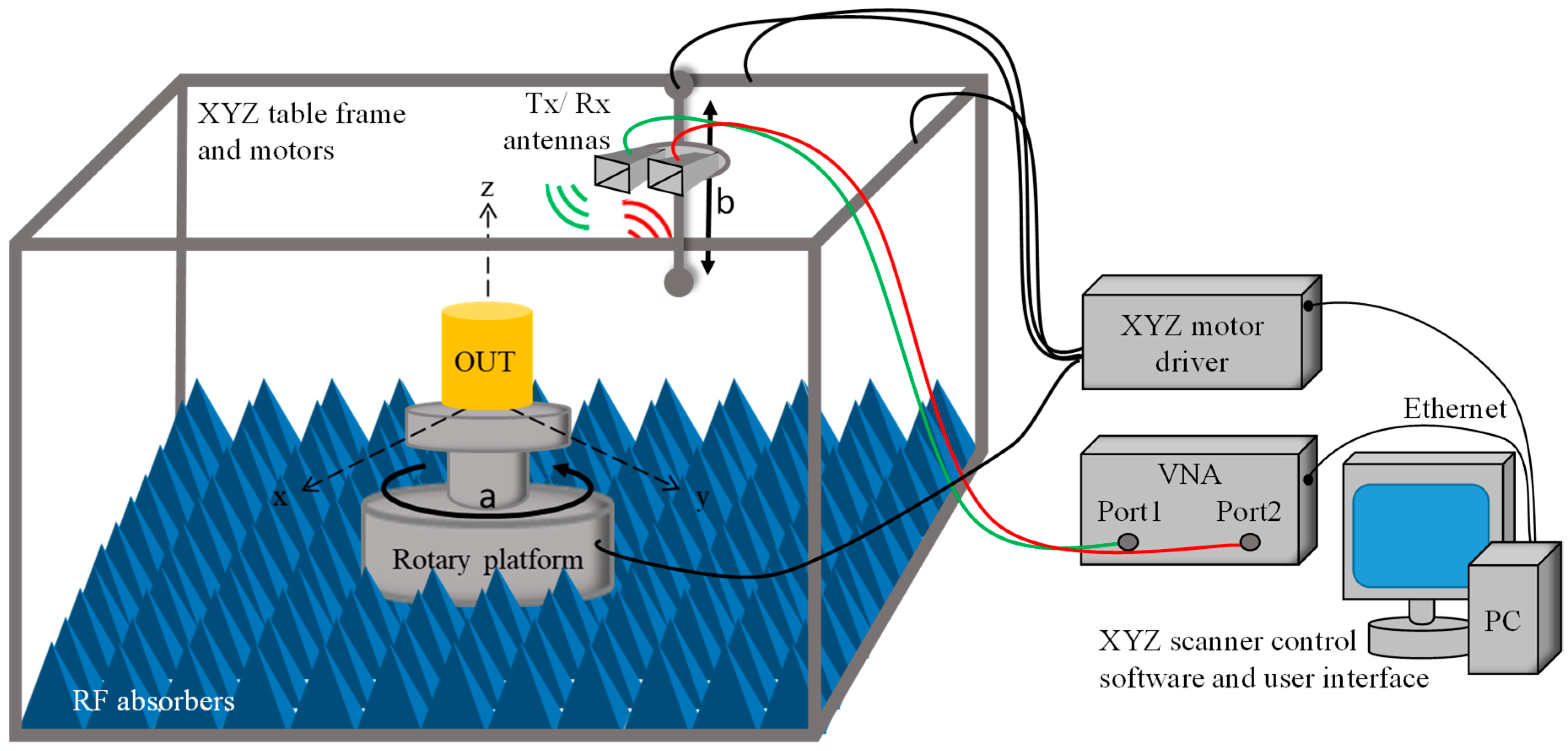
2.1. Synthetic Aperture Radar imaging

The basics of SAR processing are presented in this section. For the sake of simplicity, a two-dimensional (2D) scenario in the XY plane is considered. A 3D scenario with translation symmetry along z-axis could be assumed as well without loss of generality. Given the scattered field Escatt(f,r,φ) measured at the position (r,φ) over a certain bandwidth BW = [f1 f2], the reflectivity ρ(x’, y’) evaluated at the position (x’, y’) of the scenario-under-test is defined in Equation (1), assuming an homogeneous propagation medium:
ρ(x’, y’) = Σf=f1:f2Escatt(f,r,φ)exp(j kmediumR)
where kmedium is the wavenumber defined as kmedium = 2πf/vprop,medium, f being the frequency and vprop,medium the propagation velocity of the electromagnetic wave in a particular medium. R is the Euclidean distance between (r,φ) and (x’, y’). In case the medium is vacuum or air, k0 = 2πf/c. The center of the scenario-under-test (e.g., the center of a rotary platform in the case of a tomographic imaging system) is defined as the origin of the coordinate system. A monostatic or quasi-monostatic setup is considered, so that the transmitting and receiving antennas are placed at (r,φ). Image resolution in the radial (range) direction, Δr, is given by Equation (2):
Δr = 0.5 vprop,medium/(f2f1)
The problem can be even reduced to a one-dimensional case in the range direction, for those points satisfying x’ = r’cos(φ), y’ = r’sin(φ), so R = rr’.
Let us consider now the imaging scenario depicted in Figure 1, where the OUT is a cylindrical wax candle of diameter dOUT. The axis of the OUT is aligned with the axis of the rotary table, so that the distance between the Tx/Rx antennas and the candle surface is rdOUT/2 for any rotation angle φ. The medium surrounding the wax candle is air (kmedium = k0). Thus, the reflectivity at any point r’ ∈ [dOUT/2, r] is given by Equation (3). The range [dOUT/2, r] will be denoted as Region #1.
ρ(r’,φ) = Σf=f1:f2Escatt(f,r,φ)exp(j k0 (rr’)), r’∈[dOUT/2, r]
Next, the reflectivity for a point inside the wax candle has to be calculated taken into account the different propagation velocity inside the wax, vprop,OUT = c/(εr,OUT)1/2. Reflectivity in the interval r’∈[−dOUT/2, dOUT/2] (Region #2) is then calculated as indicated in Equation (4):
ρ(r’,φ) = Σf=f1:f2Escatt(f,r,φ)exp(j k0 (rdOUT/2)) exp(j kOUT (dOUT/2 − r’)), r’∈[−dOUT/2, dOUT/2]
And finally, for those points behind the wax candle (Region #3), the reflectivity is given by Equation (5), where the interval within the wax candle is taken into account:
ρ(r’,φ) = Σf=f1:f2Escatt(f,r,φ)exp(j k0 (rdOUTr’))exp(j kOUT dOUT), r’< −dOUT/2
Now, let us assume that neither the position nor the constitutive parameters of the OUT (the wax candle) are known. In this case, one could make use of Equation (3) to evaluate the reflectivity at any point r’. If free-space propagation is considered, a first peak of the reflectivity should appear at the interface between the air and the OUT (denoted as interface #1 in Figure 1). Similarly, a reflectivity peak should appear at any position r’ where there is an interface between two media with different constitutive parameters. But, as free-space propagation is assumed for evaluating the reflectivity at any position (Equation (1), kmedium = k0), reflectivity peaks will be shifted backwards, as illustrated in Figure 1 (dashed blue line). If the position of the interfaces and the permittivity values of the different media were known, Equations (3)–(5) could be used, resulting in a proper recovery of the reflectivity (Figure 1, solid red line).
Inaccurate recovery of the permittivity may result in inaccurate location of embedded targets in homogeneous media (e.g., tumors in breast tissue [6], or landmines buried in the ground [4]). Furthermore, depending on the imaging setup, free-space SAR approach could result in the concealed targets to be imaged outside the object where they are embedded, as it will be shown in a latter example.

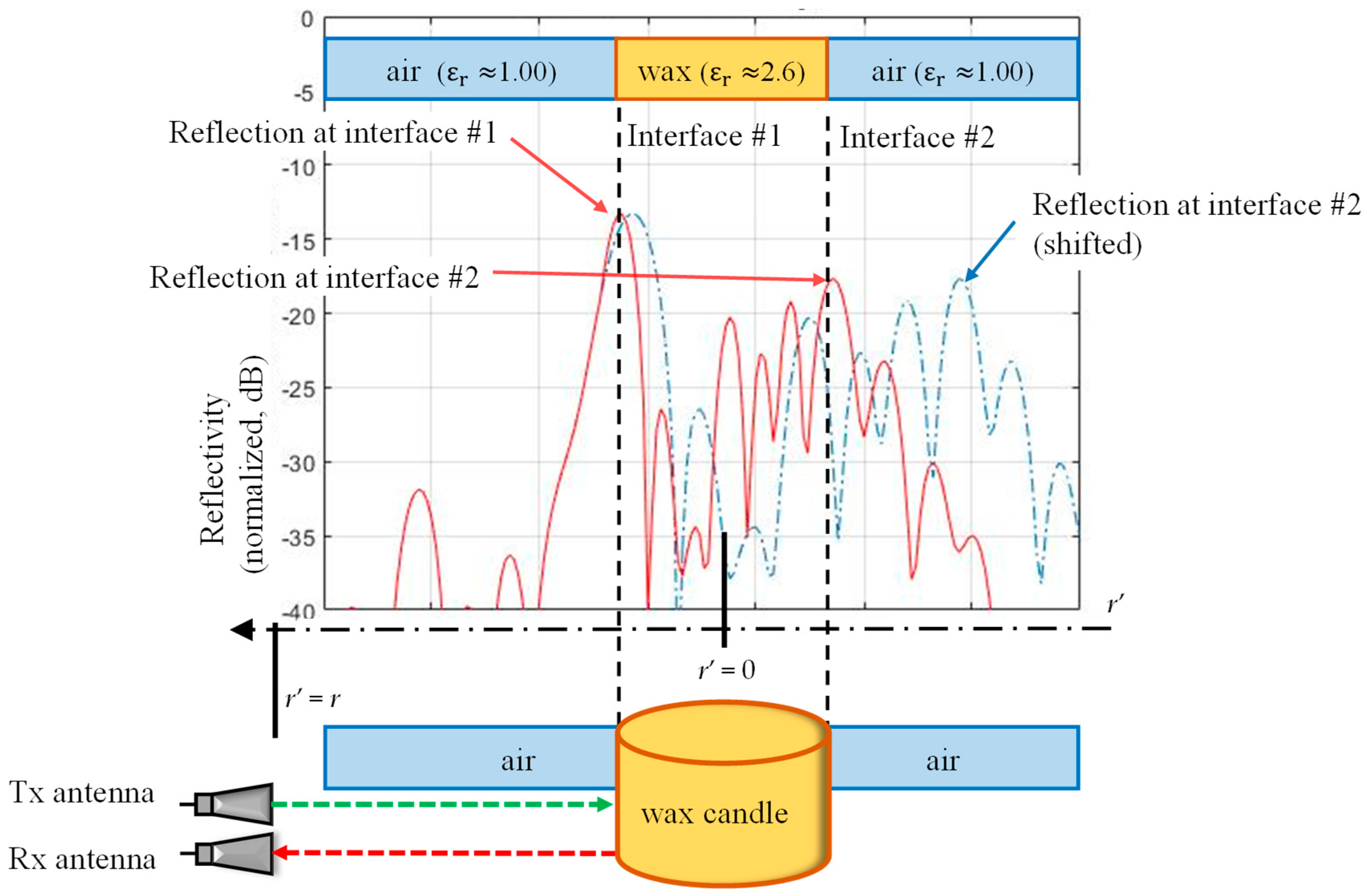
2.2. Constitutive Parameters Estimation and Range Correction

Under the assumption that the outer profile/geometry of the OUT is known, it is possible to recover the conductivity and permittivity of the OUT from the shifted reflectivity peaks. For the sake of simplicity, let us consider again the example presented in Figure 1 (a wax candle of diameter dOUT).
If the permittivity of the wax is not known, then the reflectivity calculated according to Equation (1) for all r’ with kmedium = k0 corresponds to the dashed blue line in Figure 2. From the theoretical analysis presented in Section 2.1, it is known that the reflectivity peak corresponding to the interface #2 (rear side of the candle) has to be shifted, as k0 instead of kOUT was used to calculate the reflectivity. Although its exact position cannot be estimated a priori, a search region can be defined taking into account the size of the OUT. For this example, it can be expected the reflectivity peak corresponding to the interface #2 to appear at r’ < −dOUT. The distance between the shifted reflectivity peak of interface #2 and the reflectivity peak of interface #1 is denoted as decho (Figure 2).
Next, the relationship between the delay (or phase shift) considering free-space propagation (Equation (1), kmedium = k0) and propagation through the OUT considering a permittivity estimate εr,est, yields Equation (6). An explanation about how to obtain this equation is given in [21,22]:
εr,est = (decho/dOUT)2
Note that, for the scenario considered to illustrate this methodology, no additional reference targets are required for recovering the permittivity. In this case, the shifted reflection at the interface #2 corresponds to the OUT-air interface.
Once the permittivity is estimated, Equations (3)–(5) can be applied to recover the reflectivity with the corrected propagation velocity within the OUT, so that the reflectivity peak of the interface #2 will appear at the correct position, that is, without shifting (solid red line in Figure 2).
In addition to the permittivity, an estimate of the conductivity (σOUT) can be obtained as well, by measuring the difference on the reflectivity levels at interfaces #1 and #2. The attenuation constant α (measured in Np/m) is given by Equation (7) [22]:
α = ln(|ρ(rinterface #1)|/|ρ(rinterface #2)|)/dOUT
α is related to the conductivity according to Equation (8) [22]:
σ ≈ Im{((εr)1/2 + jαc/(2πfc))2}, fc = (f1 + f2)/2
A summary of the methodology described in this section is illustrated in Figure 3.

3. Results

Validation of the proposed methodology for fast and simple estimation of constitutive parameters from SAR images is conducted in this section.

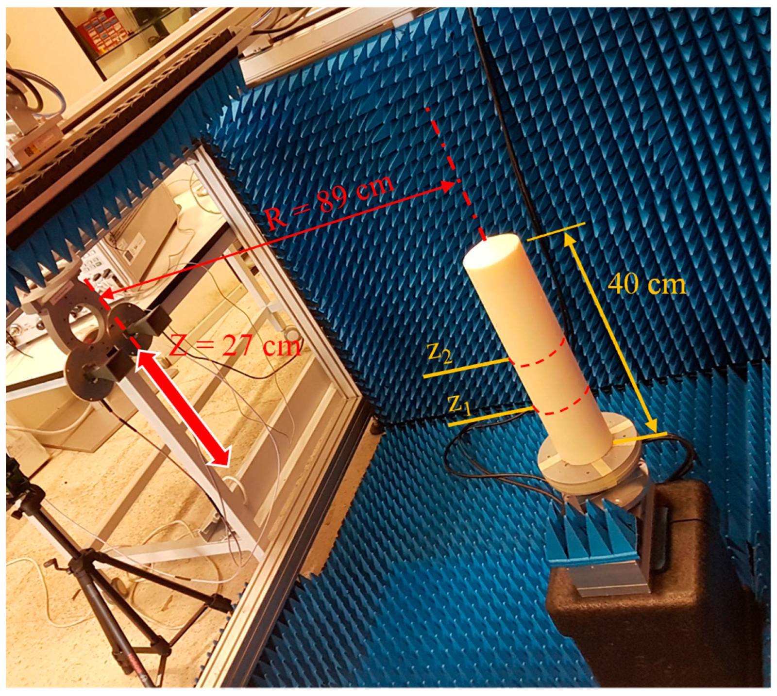
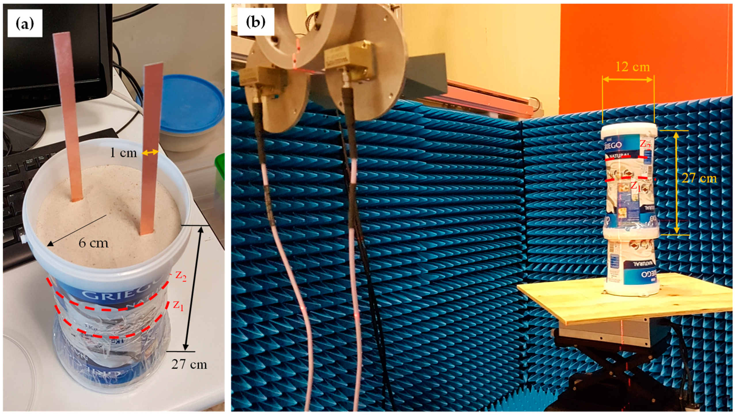
3.1. Measurement Setup
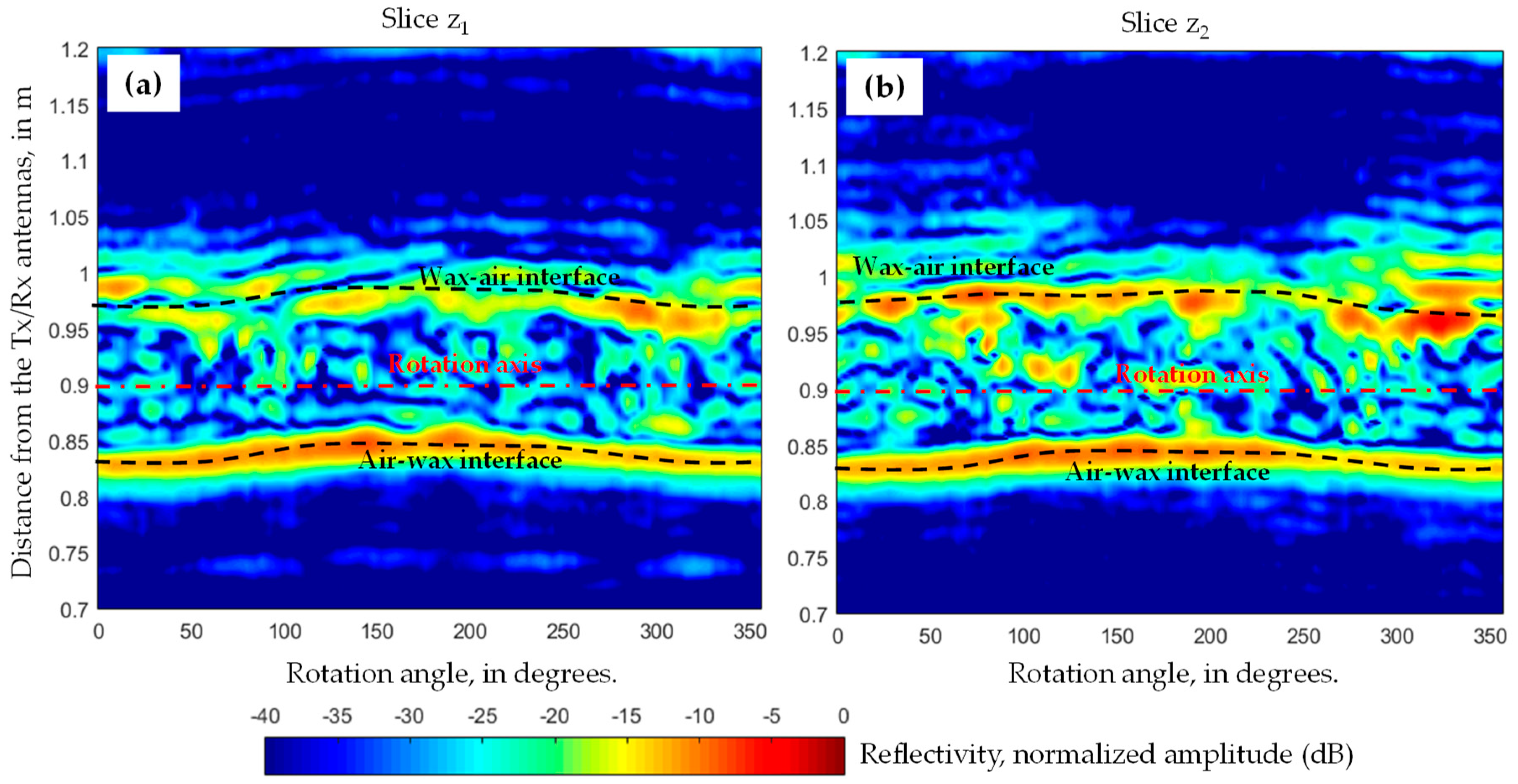
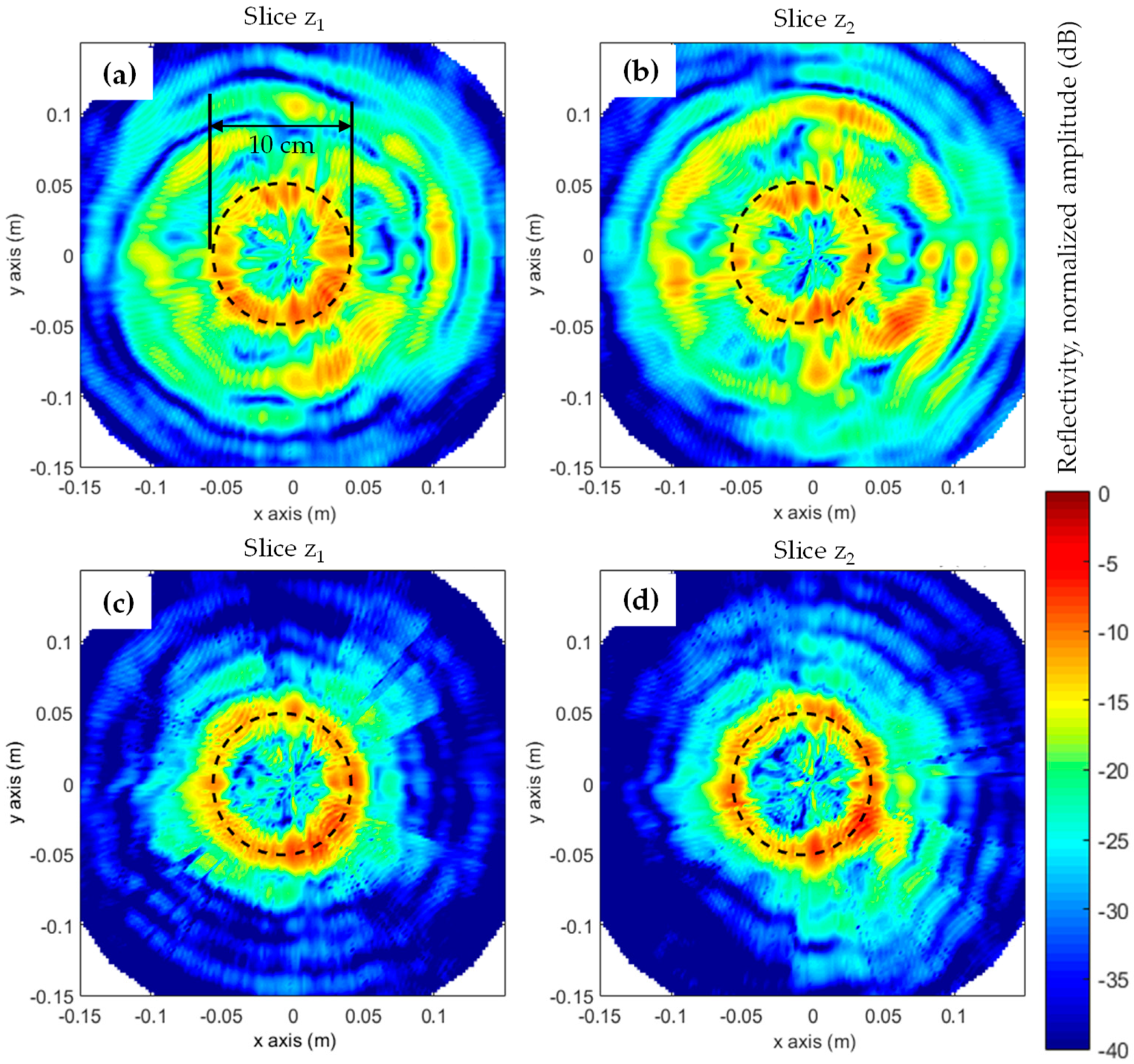
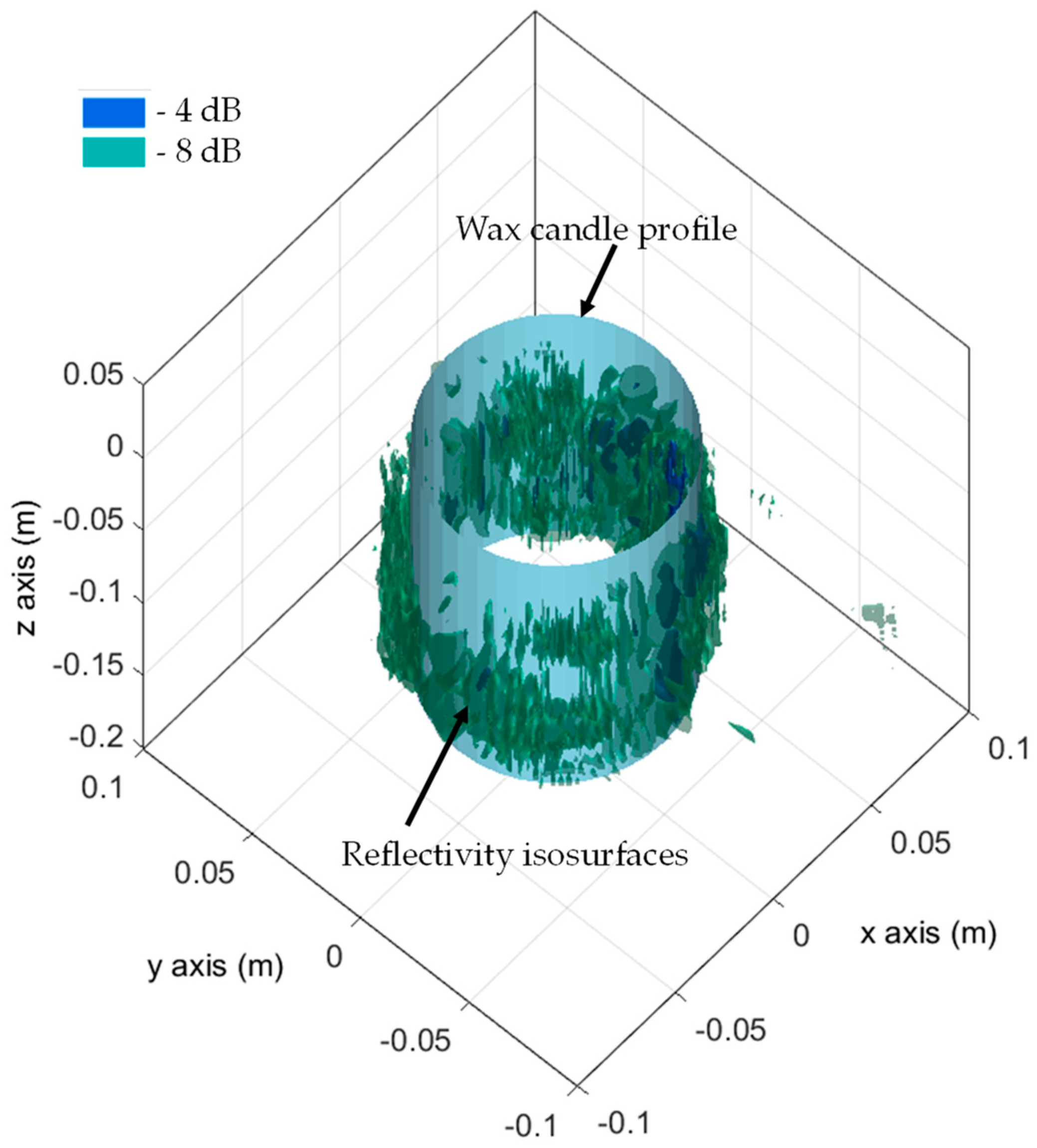
A 3D tomographic measurement setup is proposed, consisting of a rotary platform where the OUT is placed, and an XYZ positioner [24]. The Tx/Rx probe antennas (Standard Gain Horn, SGH [25]) are mounted in a quasi-monostatic configuration on a vertical slider of the XYZ positioner. Vertical (z-axis) motion is allowed along 27 cm, in 1 cm steps, while the OUT can be rotated 360°, with 1° step. With these parameters, the entire measurement of the OUT takes around 1 h and 30 min. Alignment of the Tx/Rx antennas with respect to the center of the rotary platform was conducted using a laser leveler. The distance from the rotation axis of the rotary platform to the aperture plane of the Tx/Rx antenna is 89 cm.
Tx/Rx antennas are connected to a Microwave Vector Network Analyzer (VNA) [26], as shown in the scheme of Figure 4 and in the picture of Figure 3. In order to set a reference phase for SAR imaging, calibration is done at the end of the cables connecting the VNA and the SGH antennas. A frequency band from f1 = 12 GHz to f2 = 18 GHz is selected as a trade-off between resolution and penetration of the electromagnetic waves in the targets to be tested. This bandwidth yields Δr’ = 2.5 cm resolution in range.
SGH aperture size is 5.6 × 4.4 cm [25], so DSGH = (5.6 × 4.4)1/2 = 5 cm. The far field distance is RFF = 2(DSGH)2/λ = 29.4 cm at f = 18 GHz. As the distance between the Tx/Rx antennas and the center of the rotary platform is 89 cm, then, the OUT is placed in the far field region of the antennas. Besides, for this SGH, −3 dB antenna beamwidth (θ−3dB) ranges from 25.5° at 18 GHz, to 37° at 12 GHz. That means that, at the distance of 89 cm, the θ−3dB is wider than 42.5 cm in the working frequency band, thus fully covering the area where the OUT is placed.
As the OUT is placed in the far field region of the Tx/Rx antennas, and it is fully illuminated by the antenna beams, spherical wave propagation can be assumed in the imaging domain. Note that if the OUT were placed in the near field region of the Tx/Rx antennas, the spherical wave model could result in poorer imaging results, requiring accurate characterization of the near field in the imaging domain.

3.2. Wax Candle

The first OUT selected for testing the proposed methodology for accurate SAR imaging and constitutive parameters retrieval was a wax candle, with 40 cm length and 10 cm diameter, as depicted in Figure 5. The fact of having both rotation and translation symmetry around vertical (z-) axis motivated the choice of this OUT.
Once the scattered field for each Tx/Rx position and rotation angle was measured, it was processed according to the flowchart depicted in Figure 3. The recovered reflectivity of the OUT for each rotation angle φ in the range r’ = [0.7, 1.15] at two different XY planes (or slices) z1 and z2 is shown in Figure 6. Range r’ is defined from the position of the Tx/Rx antennas, being the center of rotation (rotation axis in Figure 6) located at r’ = 0.89 m. As the constitutive parameters of the wax are not known, reflectivity is calculated using Equation (1) (kmedium = k0). The reflection at the air-wax interface (#1) can be clearly visible in Figure 6, having a mean value of |ρ(interface #1)| ≈ −10 dB = 0.32. Note that the wax candle was not perfectly centered at the rotation axis, so the reflectivity peak of the air-wax interface fluctuates between r’ = [0.83, 0.85] m. As the wax diameter is dOUT = 10 cm, the reflectivity peak of the wax-air interface (#2) can be expected to be found at r’ > [0.83 + dOUT, 0.85 + dOUT] m. For each rotation angle (φ) the maximum of the reflectivity in the range r’ = [0.95, 1.15] is registered. As observed in Figure 6, the reflectivity peak of the interface #2 ranges between r’ = [0.97, 1.01] m, with an average amplitude of |ρ(interface #1)| ≈ −15 dB = 0.18. Finally, decho is calculated as the distance between the first and second reflectivity peaks. As the OUT has a cylindrical shape, decho can be calculated individually for each rotation angle, then averaging the result, yielding decho = 0.15 m.
Now, by applying Equations (6)–(8), an estimate of the permittivity and the conductivity for the wax candle can be calculated (Equations (9)–(11)):
εr,est = (decho/dOUT)2 = (0.15 m/0.1 m)2 = 2.3
α = ln(|ρ(rinterface #1)|/|ρ(rinterface #2)|)/ dOUT = ln(0.32/0.18)/0.1 = 5.76 Np/m = 50 dB/m
σ ≈ Im{((εr,est)1/2 + jα c/(2πfc))2} = 0.06 S/m, with fc = (f1 + f2)/2 = 15 GHz
As listed in Table 1, these values are in agreement with the expected ones for paraffin (wax), as discussed in [27] (Figure 3, parameter x = 0) and in [3] (f = 9.4 GHz: εr,est = 2.17, σest = 0.03 S/m), where an integral equation-based technique was used to recover these constitutive parameters.
Apart from the constitutive parameters, the goal of the proposed methodology is to recover the geometry of the OUT. For this purpose, the (r’,φ) representation of the reflectivity has to be converted into cartesian coordinates. If the rotation axis of the rotary table is defined as z-axis, then, for each slice, the reflectivity in cartesian coordinates is given by Equation (12):
ρ(x’, y’, z’) = ρ ((r’ − R)cos(φ), (r’ − R)sin(φ), z’), with R = 89 cm.
Figure 7a,b corresponds, respectively, to the reflectivity depicted in Figure 6a,b, after applying Equation (12). While the profile of the wax candle can be noticed (R = 5 cm), several echoes outside the wax contour are observed as well. These correspond to the uncorrected position of the wax-air interface (#2), which is imaged further than its true range distance.
SAR images can be corrected by applying Equations (3)–(5), as εr,wax has been already estimated. Resulting reflectivity images in cartesian coordinates are depicted in Figure 7c,d, where it can be verified that air-wax (#1) and wax-air (#2) reflections are imaged on the contour of the wax candle.
Concerning calculation time, the number of measurement points for each slice is 360. For each rotation angle, SAR along r’ axis is calculated in ~5 ms (7 ms in the case of the corrected SAR) using a conventional laptop with no parallelization of the SAR code. Thus, the calculation time to obtain the SAR image on each slice is 18 s for uncorrected SAR and 25 s for corrected SAR. As the estimation of the conductivity and permittivity values requires less than 2 s, the overall calculation time for each slice is approximately 45 s. It must be remarked that the methodology is fully parallelizable, so that the calculation time can be decreased proportionally to the number of processors used.
It is worth mentioning that all the required information for estimating the conductivity and the permittivity, and thus being able to correct the SAR image as proved in Figure 7, is obtained just from the representation of the reflectivity assuming free-space propagation condition depicted in Figure 6.
Finally, corrected reflectivity images for different XY slices can be stacked to obtain a 3D representation of the OUT. For this example, the reconstructed geometry of the wax candle is shown in Figure 8. Graphics post-processing techniques could be applied to convert reflectivity isosurfaces into a 3D geometry model.

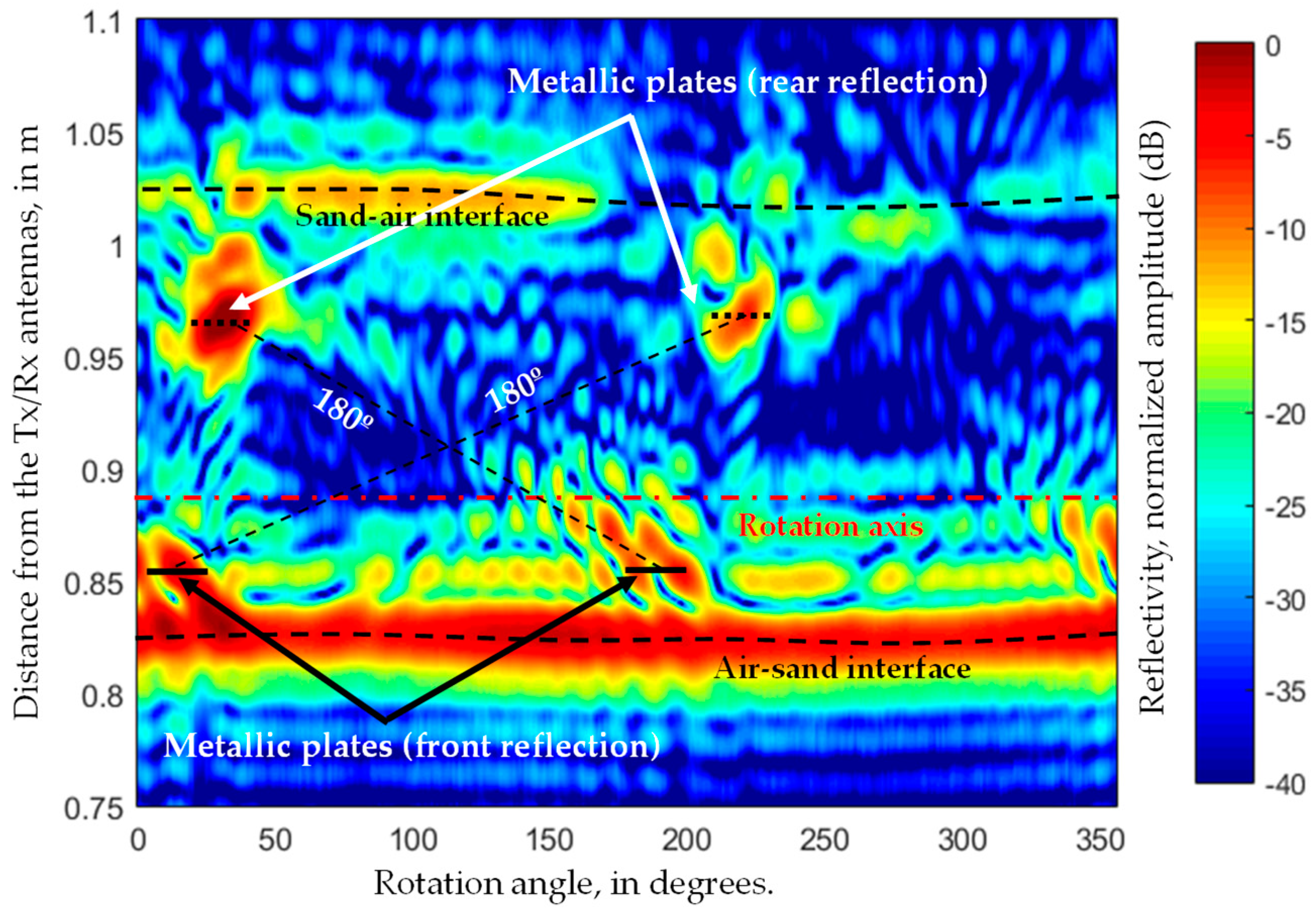
3.3. Plastic Bottle Filled with Sand

In order to remark on the consequences of not considering the permittivity of the OUT for SAR imaging, the second OUT consists of a dOUT = 12 cm diameter plastic bottle filled with sand, with two metallic plates concealed on it, as depicted in Figure 9a. The two metallic plates are placed approximately symmetrical with respect to the center of the bottle. As in the previous example, the OUT is placed on top of the rotary table (Figure 9b).
First, SAR algorithm assuming free-space propagation conditions (Equation (1)) is applied. Reflectivity for slice z1 = −13 cm as a function of the rotation angle and the distance from the Tx/Rx is depicted in Figure 10. As in the first example, the air-sand (#1) and the sand-air (#2) interfaces can be observed, together with the placement of the two metallic plates inside the plastic bottle. Note that the two metallic plates are facing the Tx/Rx antennas twice during the 360° acquisition. Thus, two main echoes of the same metallic plates (front and rear) appear in the reflectivity image, both shifted backwards proportionally to the distance between the air-sand interface and the metallic plate placement. The rear echo is more noticeable, as it is further from the air-sand interface (which partially masks the front reflection of the metallic plates).
If this reflectivity image is converted into cartesian coordinates by applying Equation (12), the image depicted in Figure 11a is obtained. Not only the sand-air interface (#2) is shifted backwards, but also the rear reflection of the metallic plates is imaged outside the sand box. The reason is that the displacement of the rear reflection due to free-space propagation conditions is greater than the distance from the metallic plates to the plastic bottle. If another slice is chosen (z2 = −7 cm), the same effect can be observed (Figure 11b). Thus, there is a clear need for using an estimate of the permittivity of the sand in order to recover a correct reflectivity image of the OUT. As in the previous example, conductivity and permittivity can be estimated from the uncorrected reflectivity depicted in Figure 10.
An analysis of Figure 10 allows estimating the air-sand interface (#1), located at r’ = 0.83 m on average, and the sand-air interface (#2), placed at r’ = 1.02 m. Thus, as decho = 19 cm and dOUT = 12 cm, the relative permittivity estimated using Equation (6) is εr,est = 2.5.
For the conductivity, values of the reflectivity within the angular range φ = [60°, 150°] can be considered, yielding |ρ(interface #1)| ≈ −5 dB = 0.56, |ρ(interface #2)| ≈ −13 dB = 0.22. From Equation (7), the attenuation is α = 7.8 Np/m = 67.6 dB/m, and, finally, the conductivity is (Equation (8)) σest = 0.08 S/m.
As a reference, typical values for sand with a moisture content below 1% is εr,est ≈ 2.4 and σ = 0.02 at 10 GHz (Figure 2 of [28]). In this example, the same sand as in [22] was used, where values of εr,est ≈ [2.7, 3.5] and σ = [0.27, 0.40] were estimated in the 3 to 6 GHz frequency band. As shown in [28], the value of these constitutive parameters tends to decay with frequency. A summary of the recovered constitutive parameters is shown in Table 1.
Once the constitutive parameters have been estimated, the corrected SAR image can be computed. SAR images corresponding to slices z1 = −13 cm and z1 = −7 cm are depicted in Figure 11c,d. Not only the contour of the plastic bottle is correctly imaged, but also the two metallic plates are found inside the area filled with sand. Note that, as observed in Figure 9, the plastic bottle is not a perfect cylinder. In the case of slice z1 the surface of the bottle is almost parallel to the Tx/Rx horn antennas aperture, whereas in the case of slice z2 the surface of the bottle is slightly tilted, so that reflection on the air-sand interface will not be fully reflected back to the Tx/Rx antennas.

4. Discussion

Results presented in Section 3 confirm the effectiveness of the proposed methodology to recover the constitutive parameters of the OUT using the imaged reflectivity assuming free-space propagation conditions. Then, the estimated reflectivity value is introduced into a modified SAR technique that takes into account the different media that compose the microwave imaging scenario, so that a corrected SAR image is produced.
With respect to similar techniques where conductivity and permittivity were retrieved from reflectivity images [21,22], the main novelty is that all the information is extracted from the SAR image of the OUT, avoiding the need of placing external references such as a metallic plate (buried or acting as background). In the proposed methodology, the challenge is the development of processing algorithms capable of extracting the information from the uncorrected SAR image, taking advantage of the a priori information about the OUT geometry. In the case of the examples presented in this contribution, rotation symmetry around vertical (z-) axis made this processing easy, as the reflectivity could be represented in cylindrical coordinates (r’,φ). For those targets with more complex geometry, pattern recognition algorithms could be used to identify and extract the position of the interfaces between media.
Recovered permittivity and conductivity values are summarized in Table 1. In the case of the permittivity, the estimated values are within the range provided by other methods based on different hardware and processing techniques. Conductivity values are more dependent on the exact composition of the medium (e.g., moisture content), so larger dispersion can be expected.
Calculation time is also a key issue for the development of inverse scattering and imaging systems. Backpropagation SAR-based techniques are by far faster than model-based methods. For the examples presented in this contribution, recovery of the final SAR image required around 45 s for each XY slice using a non-parallelized software code. Although this is not real-time imaging, it must be remarked that (i) measurement time was around 180 s per slice (360 acquisition points), and (ii) the proposed SAR-based technique is fully parallelizable. If the code is run on a 4-core processor (available in most conventional computers nowadays), calculation time would be reduced to less than 12 s per slice. The use of a Graphics Processing Unit (GPU) could result in 60–80 times speedup, as explained in [9], thus enabling real-time imaging.

5. Conclusions

A simple, fast method for microwave imaging using a SAR-based technique has been presented. The proposed methodology is capable of providing an estimate of the permittivity and conductivity of the OUT from a SAR image retrieved under free-space propagation conditions, and then, correcting the SAR image by introducing the estimated permittivity value (or, in other words, introducing the correct propagation velocity at each medium on the imaging problem). Results showed the effects of inaccurate SAR imaging, and the capability of the proposed methodology to provide accurate microwave images of the targets under test.

Author Contributions

Conceptualization, Y.Á.L.; Methodology, Y.Á.L., M.G.F. and F.L.-H.; Software, Y.Á.L. and R.G.; Measurements and Validation, Y.Á.L., M.G.F. and R.G.; Data Curation, Y.Á.L., M.G.F. and R.G.; Writing-Original Draft Preparation, Y.Á.L. and R.G.; Writing-Review & Editing, M.G.F. and F.L.-H.; Supervision, F.L.-H.

Funding

This research was partially supported by the “Ministerio de Economía y Competitividad” of Spain/FEDER under grant FPU15/06341; by the Principado de Asturias under project GRUPINN-18-000191; and by the European Union under the framework of the Erasmus+ mobility agreement between the University of Oviedo (E OVIEDO 01) and Hochschule Mannheim (D MANNHEI 03).

Conflicts of Interest

The authors declare no conflict of interest.

References

  1. Deng, Y.; Liu, X. Electromagnetic Imaging Methods for Nondestructive Evaluation Methods. Sensors 2011, 11, 11774–11808. [Google Scholar] [CrossRef] [PubMed]
  2. Cooper, K.B.; Dengler, R.J.; Llombart, N.; Thomas, B.; Chattopadhyay, G.; Siegel, P.H. THz imaging radar for standoff personnel screening. IEEE Trans. Terahertz Sci. Technol. 2011, 1, 169–182. [Google Scholar] [CrossRef]
  3. Álvarez, Y.; García-Fernández, M.; Poli, L.; García-González, C.; Rocca, P.; Massa, A.; Las-Heras, F. Inverse Scattering for Monochromatic Phaseless Measurements. IEEE Trans. Instrum. Meas. 2017, 66, 45–60. [Google Scholar] [CrossRef] [Green Version]
  4. García-Fernández, M.; Álvarez-López, Y.; Arboleya-Arboleya, A.; González-Valdés, B.; Rodríguez-Vaqueiro, Y.; Las-Heras Andrés, F.; Pino García, A. Synthetic Aperture Radar Imaging System for Landmine Detection Using a Ground Penetrating Radar on Board a Unmanned Aerial Vehicle. IEEE Access 2018, 6, 45100–45112. [Google Scholar] [CrossRef]
  5. Narayanan, R.M.; Gebhardt, E.T.; Broderick, S.P. Through-Wall Single and Multiple Target Imaging Using MIMO Radar. Electronics 2017, 6, 70. [Google Scholar] [CrossRef]
  6. Elahi, M.A.; O’Loughlin, D.; Lavoie, B.R.; Glavin, M.; Jones, E.; Fear, E.C.; O’Halloran, M. Evaluation of Image Reconstruction Algorithms for Confocal Microwave Imaging: Application to Patient Data. Sensors 2018, 18, 1678. [Google Scholar] [CrossRef] [PubMed]
  7. Zhuge, X.; Yarovoy, A.G. A sparse aperture MIMO-SAR-based UWB imaging system for concealed weapon detection. IEEE Trans. Geosci. Remote Sens. 2011, 49, 509–518. [Google Scholar] [CrossRef]
  8. Soumekh, M. Bistatic synthetic aperture radar inversion with application in dynamic object imaging. IEEE Trans. Signal Process. 1991, 39, 2044–2055. [Google Scholar] [CrossRef]
  9. Lopez-Portugues, M.; Alvarez-Lopez, Y.; Lopez-Fernandez, J.A.; Garcia-Gonzalez, C.; Ayestaran, R.G.; Las-Heras Andres, F. A multi-GPU sources reconstruction method for imaging applications. Prog. Electromagn. Res. 2013, 136, 703–724. [Google Scholar] [CrossRef]
  10. Lin, C.Y.; Kiang, Y.W. Inverse scattering for conductors by the equivalent source method. IEEE Trans. Antennas Propag. 1996, 44, 310–316. [Google Scholar] [CrossRef]
  11. Woten, D.; Hajihashemi, M.R.; Hassan, A.M.; El-Shenawee, M. Experimental microwave validation of level set reconstruction algorithm. IEEE Trans. Antennas Propag. 2010, 58, 230–233. [Google Scholar] [CrossRef]
  12. Eskandari, A.R.; Naser-Moghaddasi, M.; Eskandari, M. Reconstruction of Shape and Position for Scattering Objects by Linear Sampling Method. Int. J. Soft Comput. Eng. 2012, 2, 2231–2307. [Google Scholar]
  13. Caorsi, S.; Donelli, M.; Massa, A. Detection, location, and imaging of multiple scatterers by means of the iterative multiscaling method. IEEE Trans. Microw. Theory Tech. 2004, 52, 1217–1228. [Google Scholar] [CrossRef]
  14. Rocca, P.; Benedetti, M.; Donelli, M.; Franceschini, D.; Massa, A. Evolutionary optimization as applied to inverse scattering problems. Inverse Probl. 2009, 25, 123003. [Google Scholar] [CrossRef] [Green Version]
  15. Gonzalez-Valdes, B.; Alvarez, Y.; Martinez-Lorenzo, J.A.; Las-Heras, F.; Rappaport, C.M. On the Combination of SAR and Model Based Techniques for High-Resolution Real-Time Two-Dimensional Reconstruction. IEEE Trans. Antennas Propag. 2014, 62, 5180–5189. [Google Scholar] [CrossRef] [Green Version]
  16. Fallahpour, M.; Case, J.T.; Ghasr, M.T.; Zoughi, R. Piecewise and Wiener filter-based SAR techniques for monostatic microwave imaging of layered structures. IEEE Trans. Antennas Propag. 2014, 62, 282–294. [Google Scholar] [CrossRef]
  17. Laviada, J.; Wu, B.; Ghars, M.T.; Zoughi, R. Nondestructive Evaluation of Microwave-Penetrable Pipes by Synthetic Aperture Imaging Enhanced by Full-Wave Field Propagation Model. IEEE Trans. Instrument. Meas. 2018, 1–8, in press. [Google Scholar] [CrossRef]
  18. Robinson, D.A.; Jones, S.B.; Wraith, J.M.; Or, D.; Friedman, S.P. A Review of Advances in Dielectric and Electrical Conductivity Measurement in Soils Using Time Domain Reflectometry. Vadose Zone J. 2003, 2, 444–475. [Google Scholar] [CrossRef]
  19. Garret, J.D.; Fear, E.C. Average Dielectric Property Analysis of Complex Breast Tissue with Microwave Transmission Measurements. Sensors 2015, 15, 1199–1216. [Google Scholar] [CrossRef] [PubMed]
  20. Costa, F.; Borgese, M.; Degiorgi, M.; Monorchio, A. Electromagnetic Characterisation of Materials by Using Transmission/Reflection (T/R) Devices. Electronics 2017, 6, 95. [Google Scholar] [CrossRef]
  21. Gonzalez-Valdes, B.; Alvarez-Lopez, Y.; Martinez-Lorenzo, J.A.; Las Heras, F.; Rappaport, C.M. SAR processing for profile reconstruction and characterization of dielectric objects on the human body surface. Prog. Electromagn. Res. 2013, 138, 269–282. [Google Scholar] [CrossRef]
  22. Álvarez-López, Y.; García-Fernández, M.; Arboleya, A.; González-Valdés, B.; Rodríguez-Vaqueiro, Y.; Las-Heras, F.; Pino García, A. SAR-based technique for soil permittivity estimation. Int. J. Remote Sens. 2017, 38, 5168–5185. [Google Scholar] [CrossRef]
  23. López-Rodríguez, P.; Escot-Bocanegra, D.; Poyatos-Martínez, D.; Weinmann, F. Comparison of Metal-Backed Free-Space and Open-Ended Coaxial Probe Techniques for the Dielectric Characterization of Aeronautical Composites. Sensors 2016, 16, 967. [Google Scholar] [CrossRef] [PubMed]
  24. Arboleya, A. Novel XYZ Scanner-Based Radiation and Scattering Measurement Techniques for Antenna Diagnostics and Imaging Applications. Ph.D. Thesis, Universidad de Oviedo, Oviedo, Spain, 2016. Available online: http://digibuo.uniovi.es/dspace/bitstream/10651/40222/1/TD_AnaArboleya.pdf (accessed on 12 October 2018).
  25. Bell Electronics. Narda 639 Standard Gain Horn, 12.4 to 18 GHz. Available online: https://www.bellnw.com/manufacturer/Narda/639.htm (accessed on 5 October 2018).
  26. Keysight. N5247A PNA-X Microwave Network Analyzer. Available online: https://www.keysight.com/en/pdx-x201825-pn-N5247A/pna-x-microwave-network-analyzer-67-ghz?cc=EN&lc=eng (accessed on 5 October 2018).
  27. Bayrajdar, H. Complex permittivity, complex permeability and microwave absorption properties of ferrite-paraffin polymer composites. J. Magn. Magn. Mater. 2011, 323, 1882–1885. [Google Scholar] [CrossRef]
  28. Abdelgwad, A.H.; Said, T.M. Measured dielectric Permittivity of Contaminated sandy soils at Microwave Frequency. J. Microw. Optoelectron. Electromagn. Appl. 2016, 15, 115–122. [Google Scholar] [CrossRef]
Figure 1. Illustration of the reflectivity delay due to the consideration of propagation in free-space, and comparison with corrected reflectivity when considering true permittivity (εr).
Electronics 07 00373 g001
Figure 2. Methodology to estimate the permittivity of the object-under-test (OUT) (εr,est) from scattered field measurements given the thickness of the OUT (dOUT).
Electronics 07 00373 g002
Figure 3. Picture of the measurement setup and flowchart of the Synthetic Aperture Radar (SAR)-based technique for microwave imaging and constitutive parameters characterization.
Electronics 07 00373 g003
Figure 4. Scheme of the measurement for dielectric objects imaging using a rotary platform and vertical slider. Tx and Rx antennas are placed according to a quasi-monostatic configuration with respect to the OUT. Full (360°) angular rotation (a) is allowed. Vertical motion range is b = 27 cm.
Electronics 07 00373 g004
Figure 5. Picture of the wax candle placed on the rotary platform.
Electronics 07 00373 g005
Figure 6. Reflectivity calculated for each observation angle as a function of the distance from the Tx/Rx antennas, for two different XY slices ((a) z1 = −12 cm and (b) z2 = −5 cm with respect to the top of the wax candle). Air-wax (front reflection) and wax-air (rear reflection) interfaces are noticed.
Electronics 07 00373 g006
Figure 7. Polar representation of the reflectivity for two different XY slices (z1 = −12 cm and z2 = −5 cm with respect to the top of the wax candle). (a,b) Without dielectric delay correction. (c,d) After dielectric delay correction, considering εr,est = 2.3. Dashed line represents the true contour of the wax candle.
Electronics 07 00373 g007
Figure 8. 3D representation of the recovered reflectivity of the wax candle, after dielectric delay correction.
Electronics 07 00373 g008
Figure 9. (a) Picture of the plastic box filled with sand, with two metallic plates embedded. (b) Picture of the OUT placed on the rotary platform.
Electronics 07 00373 g009
Figure 10. Reflectivity calculated for each observation angle as a function of the distance from the Tx/Rx antennas, for a XY slice (z1 = −13 cm with respect to the top of the plastic box). Air-sand (front reflection) and sand-air (rear reflection) interfaces are noticed, as well as the stronger reflection in the metallic plates.
Electronics 07 00373 g010
Figure 11. Polar representation of the reflectivity for two different XY slices (z1 = −13 cm and z2 = −7 cm with respect to the top of the plastic bottle). (a,b) Without dielectric delay correction. (c,d) After dielectric delay correction, considering εr,est = 2.5. Dashed line represents the true contour of the plastic bottle. Solid line represents the true position of the metallic plates. In (a,b), the straight dashed lines indicate the location of the imaged metallic plates, which appear outside the plastic box contour due to the dielectric delay.
Electronics 07 00373 g011
Table 1. Constitutive parameters of the media considered in the examples. Comparison with other techniques at microwave frequencies.
MaterialFrequency (GHz)Permittivity (εr)Conductivity (σ) (S/m)MethodReference
Wax (paraffin)12–182.3 ± 0.20.06 ± 0.02Backpropagation SARThis contribution
Wax (paraffin)9–152.20.35X-ray powder diffraction analysis[27]
Wax (paraffin)9.42.170.03Model-based monochromatic inverse scattering[3]
Sand12–182.5 ± 0.20.08 ± 0.02Backpropagation SARThis contribution
Sand3–6[2.7, 3.5][0.27, 0.4]Backpropagation SAR, with reference target[22]
SandUp to 102.4 ± 0.20.02 ± 0.005Coaxial probe[28]

