Unmanned Aerial Vehicle Recognition Based on Clustering by Fast Search and Find of Density Peaks (CFSFDP) with Polarimetric Decomposition

Abstract

Unmanned aerial vehicles (UAV) have become vital targets in civilian and military fields. However, the polarization characteristics are rarely studied. This paper studies the polarization property of UAVs via the fusion of three polarimetric decomposition methods. A novel algorithm is presented to classify and recognize UAVs automatically which includes a clustering method proposed in “Science”, one of the top journals in academia. Firstly, the selection of the imaging algorithm ensures the quality of the radar images. Secondly, local geometrical structures of UAVs can be extracted based on Pauli, Krogager, and Cameron polarimetric decomposition. Finally, the proposed algorithm with clustering by fast search and find of density peaks (CFSFDP) has been demonstrated to be better than the original methods under the various noise conditions with the fusion of three polarimetric decomposition methods.

1. Introduction

Radar is an electronic system that utilizes electromagnetic waves to obtain the attribute information of the object which consists of velocity and range [1,2]. The potential targets that are often sensed with radar are vessels, aircraft, spacecraft, civilian vehicles, military tanks, terrain, and so on [3]. The automatic target recognition (ATR) [4,5,6] system takes advantage of the information reflected from the targets, by analyzing electromagnetic characteristic and extracting features to classify and recognize the objects. Radar automatic target recognition continues to advance with the development of radar hardware and information processing technology. Applications of broadband and multi-polarization technologies not only enhance the comprehension of target attribute information, but also bring a challenge of information processing [7].

The research on man-made targets has attained significant achievements in SAR/ISAR imaging and processing [8,9]. Dungan et al. focused on civilian vehicle radar data and investigated the signature of cars which had been adopted to the reconstruction of elevation [10]. In Reference [11], the study reveals the characteristic of civilian cars in SAR imaging with noise and classifies ten kinds of vehicles under various signal-to-noise ratio (SNR) conditions. Fuller et al. established a high-frequency model to solve the problems of parameter estimation and scatter classification in the spatial domain with simulated data [12]. In addition, the literature [13] established a forward approach of parametric scattering center model in the ATR system which had achieved great agreement between the simulation and experimental data. In the application of wide-angle SAR/ISAR, Jianxiong Zhou et al. reconstructed 3D tank and slice-like targets with a single elevation [14]. Dal-Jae Yun presented a 3D scattering center extraction algorithm with a fast Fourier transform-based scheme which has been applied to tank models [15]. Though great progress has been made for the analysis of those targets with simple structures, more work should be made for analyzing objects with complex structures or even with various materials like UAVs.

The polarization characteristic can be utilized to extract the structure characteristic of the man-made target. A Huynen Parametric decomposition technique has been applied to estimate the height profile of civilian vehicles and demonstrate the target structural mechanism [16]. Reference [17] developed a method of feature extraction and parametric estimation for scattering centers which can be utilized to simplify the description of the electromagnetic property of the target. Reference [18] proposed a novel algorithm to retrieve the geometrical structure of man-made targets in images with Cameron decomposition and had shown the potential to estimate the coordinates and the types of scattering centers. An original polarimetric coherent target decomposition method in SAR images which consists of data simulated by XPATCH software with different noise and the robustness is proved under strong noise [19]. Despite polarimetric decomposition methods bring convenience to the analysis of the target, the limitation of the single decomposition method needs to be addressed.

The study on UAVs, a typical kind of man-made targets, has become a frontier issue in recent years. As far as UAVs have been concerned, a motion compensation algorithm was proposed by Xing et al. to minimize the 3D motion error [20]. In Reference [21], micro-Doppler signatures of UAVs with rotating rotors were analyzed which could be utilized for the recognition of unmanned gyroplanes. X-band tracking radar was applied to measure the radar cross-section of the UAV in flight and the dynamic effects were considered [22]. In Reference [23], different micro-UAVs in flight were measured in various realistic environments and micro-Doppler characteristics were discussed. Pieraccini from the University of Florence reconstructed the 2D and 3D images of a small quadcopter with the blades not rotating [24]. However, there are few studies on the polarization characteristics of the UAV target and its component structure. This paper focuses on the polarization features of simulated and measured electromagnetic data of UAVs and a novel algorithm has been proposed to classify UAVs.

In this paper, on the basis of CFSFDP and polarimetric decomposition methods, we propose a novel clustering algorithm to recognize UAVs. The algorithm can not only obtain the physical structure, but also classify UAVs precisely. The advantages of the proposed method are shown as follows:

Classifying the UAVs automatically without prior information;

• Better performance under conditions of different SNRs in contrast with other algorithms;
• Extraction of the local geometrical structure of UAVs based on polarimetric decomposition.

The framework of contents in this paper is shown in Figure 1. Section 1 introduces the background of UAV recognition and the structure of this paper. Section 2 and Section 3 present the imaging algorithms and coherent polarimetric decomposition methods; Section 4 introduces the methodology of clustering by fast search and find of density peaks; Section 5 provides the procedure of the proposed novel algorithm which is designed based on contents from Section 2, Section 3 and Section 4; Experimental results and conclusions are shown in Section 6 and Section 7 respectively.

2. Imaging Algorithm

Imaging is an indispensable operation before extracting features and recognizing targets. Two-dimensional Fourier transform and Convolution Back-projection (CBP) algorithm have been employed in this paper. These two methods are widely used in the research of ISAR imaging and have their advantages respectively. The process of 2D Fourier transform is straightforward while the consumptions of computing resources are considerably huge. The methodology of the convolution back-projection algorithm has been reviewed in Reference [25].

2.1. Polarimetric Matrix and the Signal Model of Radar Imaging

Polarimetric inverse synthetic aperture radar (PolISAR) obtains more information in the imaging scene than conventional radar. Conventional radar has only one or two polarimetric channels, whereas PolISAR has four channels. For PolISAR [26], in the horizontal and vertical polarization bases (H, V), the acquired fully polarimetric data could form a scattering matrix with representation as

$$S=\left[\begin{array}{cc}{S}_{HH}& S_{HV}\\ S_{VH}& S_{VV}\end{array}\right]$$

(1)

where $S_{HV}$ is the backscattered coefficient from the vertical transmitting and horizontal receiving polarization, $S_{HH}$ is the backscattered coefficient transmitted and received both from the horizontal polarization. The other backscattered coefficients are similarly defined.

According to the definition of radar cross section ${\sigma }_{pq}$ and the reciprocity theorem [27]

$$S_{HV}=S_{VH}$$

(2)

$${\sigma }_{pq}=4\pi {\left|S_{pq}\right|}^{2}p,q=H,V$$

(3)

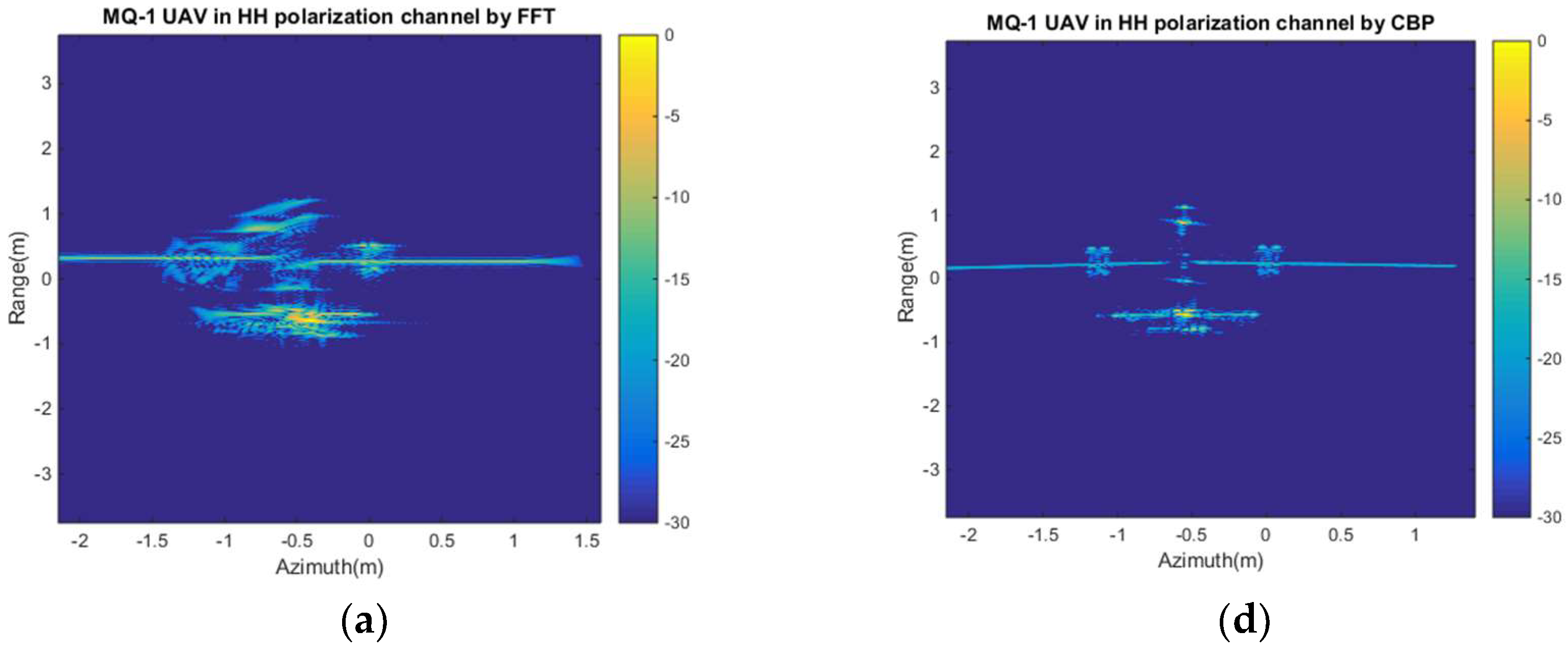
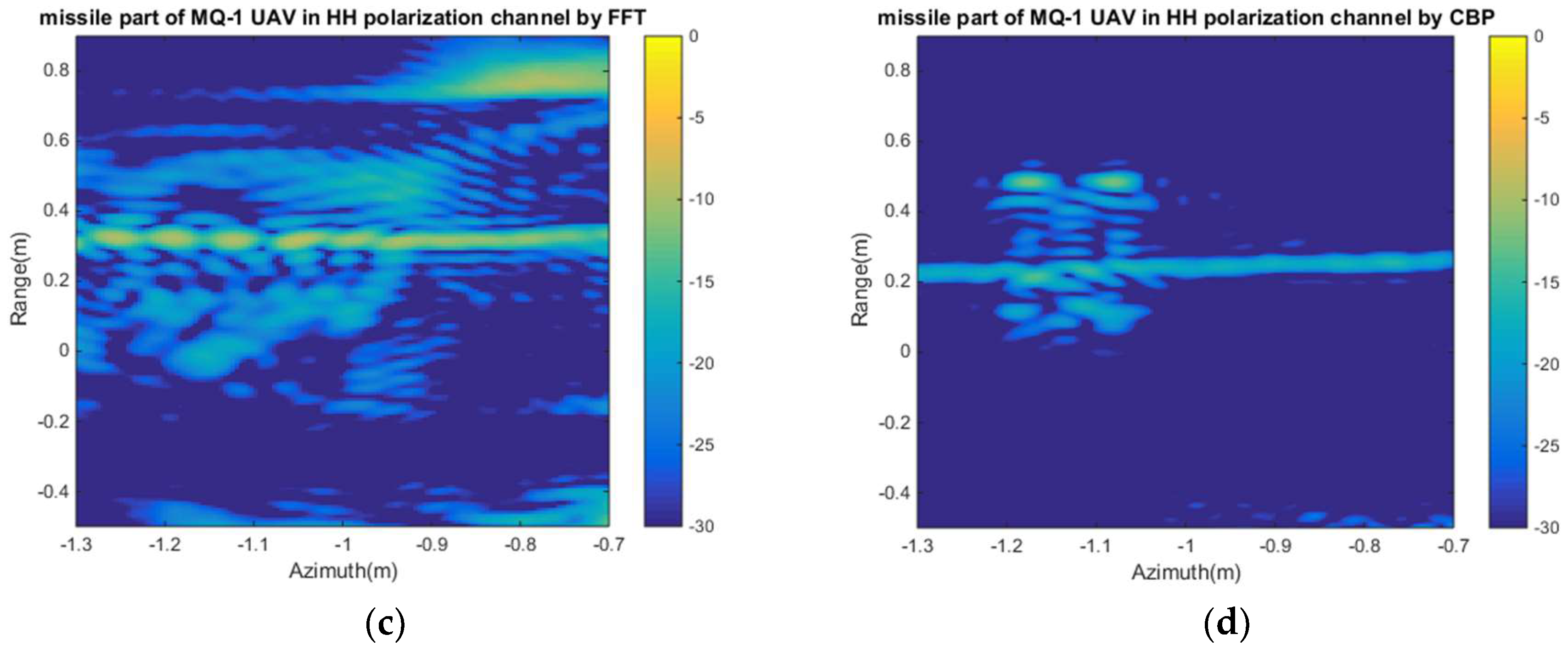
2.2. 2D Fourier Transform Algorithm

In Cartesian coordinates, $g\left(x,y\right)$ denotes the ground reflectivity function and the 2D Fourier transform [28] is defined as follows:

$$G\left(X,Y\right)={\displaystyle {\int }_{-\infty }^{+\infty }{\displaystyle {\int }_{-\infty }^{+\infty }g\left(x,y\right)e^{-j\left(Xx+Yy\right)}}}dxdy$$

(4)

And

$$g\left(x,y\right)=\frac{1}{4{\pi }^2}{\displaystyle {\int }_{-\infty }^{+\infty }{\displaystyle {\int }_{-\infty }^{+\infty }G\left(X,Y\right)e^{-j\left(Xx+Yy\right)}}}dXdY$$

(5)

Let $\left(w,\theta \right)$ represent the polar coordinates in the $\left(u,v\right)$ plane. $G\left(w,\theta \right)$ denotes the value of $G\left(X,Y\right)$ along a line at an angle $\theta$ with $y$-axis.

The reconstructed image $\widehat{g}\left(x,y\right)$ can be expressed as

$$\widehat{g}\left(x,y\right)={\displaystyle {\int }_{w_1}^{w_2}{\displaystyle {\int }_{-\left({\theta }_m/2\right)}^{{\theta }_m/2}G\left(w,\theta \right)e^{-jw\left(x\cos \theta +y\sin \theta \right)}}}d\theta dw$$

(6)

$$\widehat{g}\left(r,\theta \right)={\displaystyle {\int }_{w_1}^{w_2}{\displaystyle {\int }_{-\left({\theta }_m/2\right)}^{{\theta }_m/2}G\left(w,\theta \right)e^{-jwr}}}d\theta dw$$

(7)

3. Polarimetric Decomposition Methods

The physical structural characteristics of the target can be obtained effectively by polarimetric decomposition. The polarimetric decomposition methods of the target are mainly divided into coherent decomposition and incoherent decomposition. The incoherent decomposition discusses the characteristics of the change of the target under time-varying conditions, and the model is quite complex. This paper focuses on the UAV target with coherent decomposition methods. Coherent decomposition methods consist of Pauli decomposition, Krogager decomposition, and Cameron decomposition.

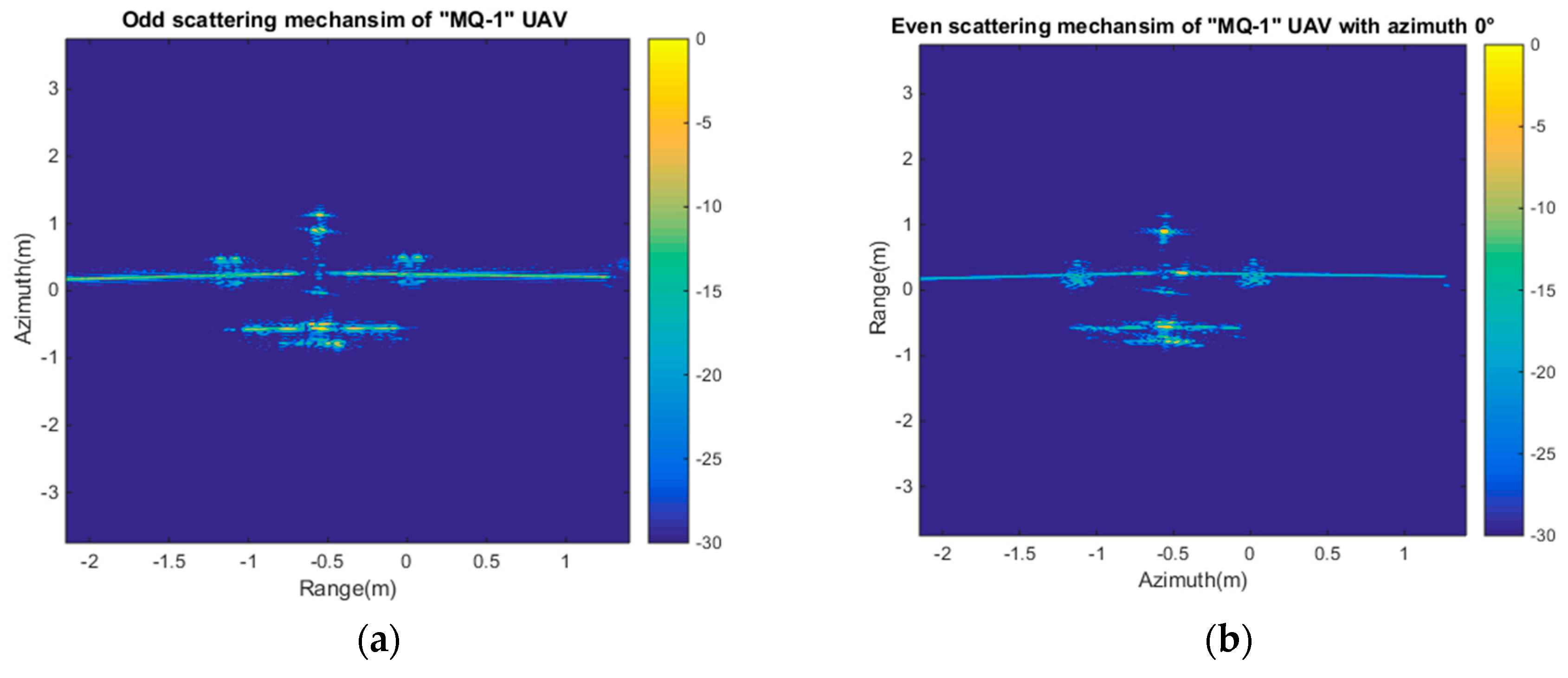
3.1. Pauli Decomposition

The Pauli decomposition decomposes the scattering matrix $S$ into three simple scattering mechanisms that represent odd-bounce scattering, even-bounce scattering, and asymmetric component scattering [29,30,31]. The even-bounce scattering can be further divided into dihedral targets with azimuth angles of 0° and 45°.

The scattering matrix of the target can be rewritten as

$$S=\frac{\alpha }{\sqrt{2}}\left[\begin{array}{cc}1& 0\\ 0& 1\end{array}\right]+\frac{\beta }{\sqrt{2}}\left[\begin{array}{cc}0& 1\\ 1& 0\end{array}\right]+\frac{\chi }{\sqrt{2}}\left[\begin{array}{cc}1& 0\\ 0& -1\end{array}\right]+\frac{\delta }{\sqrt{2}}\left[\begin{array}{cc}0& -j\\ j& 0\end{array}\right]$$

(8)

As mentioned in the previous section, the polarimetric scattering matrix consists of four elements: $S_{HH}$, $S_{HV}$, $S_{VH}$ and $S_{VV}$. When the reciprocity condition is satisfied, $S_{HV}=S_{VH}$ can be obtained. The four complex numbers are $\alpha$, $\beta$, $\chi$ and $\delta$, they are thus given by

$$\alpha =\frac{S_{HH}+S_{VV}}{\sqrt{2}}$$

(9)

$$\beta =\frac{S_{HV}+S_{VH}}{\sqrt{2}}$$

(10)

$$\chi =\frac{S_{HH}-S_{VV}}{\sqrt{2}}$$

(11)

$$\delta =j\frac{S_{HV}-S_{VH}}{\sqrt{2}}$$

(12)

When the limit of monostatic and reciprocity is satisfied, (8) can be simplified as

$$S=\frac{\alpha }{\sqrt{2}}\left[\begin{array}{cc}1& 0\\ 0& 1\end{array}\right]+\frac{\beta }{\sqrt{2}}\left[\begin{array}{cc}0& 1\\ 1& 0\end{array}\right]+\frac{\chi }{\sqrt{2}}\left[\begin{array}{cc}1& 0\\ 0& -1\end{array}\right]$$

(13)

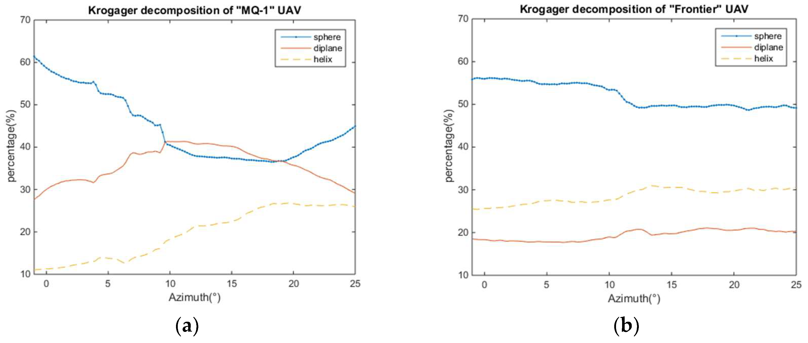
3.2. Krogager Decomposition

The Krogager decomposition [29,30] characterizes the scattering electromagnetic properties of the complex object with three basic scattering mechanisms, namely, the sphere, the dihedral with azimuth angle $\phi$, and the helix.

$$S=e^{j\psi }\left\{k_H{S}_{he}+e^{j{\psi }_s}{k}_S{S}_{sp}+k_D{S}_{di}\right\}$$

(14)

where

$$S_{sp}=\left[\begin{array}{cc}1& 0\\ 0& 1\end{array}\right],S_{he}=\left[\begin{array}{cc}1& \mp j\\ \mp j& -1\end{array}\right],S_{di}=\left[\begin{array}{cc}\cos 2\phi & \sin 2\phi \\ \sin 2\phi & -\cos 2\phi \end{array}\right].$$

$S_{sp}$, $S_{he}$, and $S_{di}$ represent the scattering matrices corresponding to a sphere, helix, and dihedral. $k_S$, $k_D$ and $k_H$, are denoted as the contribution of three scattering mechanisms of the specific target. $\phi$ is the azimuth of the dihedral, $\psi$ represents the absolute phase, ${\psi }_s$ shows the relative phase difference between the scattering component corresponding to the minimum unit sphere and other scattering mechanisms.

After the operation under the circular polarization [29], the scattering matrix $S$ is represented as

$$S=e^{j\psi }\left[\begin{array}{cc}{e}^{j{\psi }_S}{k}_S+k_H{e}^{\mp j2\phi }+k_D\cos 2\phi & j{k}_H{e}^{\mp j2\phi }\pm k_D\sin 2\phi \\ j{k}_H{e}^{\mp j2\phi }\pm k_D\sin 2\phi & e^{j{\psi }_S}{k}_S-k_H{e}^{\mp j2\phi }-k_D\cos 2\phi \end{array}\right]$$

(15)

The Krogager decomposition decomposes the target into three basic scattering mechanisms that simplify the interpretation and analysis of the target physical properties.

3.3. Cameron Decomposition

Cameron decomposition of radar targets has two characteristics: symmetry and reciprocity [31,32]. It is different from Pauli decomposition. Pauli decomposition decomposes the target scatter into several simple scattering mechanisms. Cameron decomposition first decomposes the scattering matrix into reciprocal and nonreciprocal parts. The reciprocal part is then divided into symmetrical and asymmetrical parts based on symmetry. The expression of Cameron decomposition is as follows:

$$S=a\left\{{\widehat{S}}_{nonrec}\sin {\theta }_{rec}+\cos {\theta }_{rec}\left\{{\widehat{S}}_{sym}^{\max }\cos {\tau }_{sym}+{\widehat{S}}_{sym}^{\min }\sin {\tau }_{sym}\right\}\right\}$$

(16)

where

$$a={\Vert \overrightarrow{S}\Vert }_2^2=Span\left(S\right)$$

(17)

The angle ${\theta }_{rec}$ represents the proportion of reciprocal scatter and ${\tau }_{sym}$ shows the proportion of symmetric part of the scatter. The vector ${\widehat{S}}_{nonrec}$ is the representation of the normalized non-reciprocal scatter, ${\widehat{S}}_{sym}^{\max }$ corresponds to the portion of the normalized symmetric scatter, ${\widehat{S}}_{sym}^{\min }$ is denoted as the vector form of the normalized asymmetric scatter.

Cameron decomposition first uses the Pauli decomposition to weight the sum of the target’s scattering matrix, then transforms the scattering matrix into the vector form [33]:

$$\stackrel{\rightharpoonup }{S}=\frac{\alpha }{\sqrt{2}}\left[\begin{array}{c}1\\ 0\\ 0\\ 1\end{array}\right]+\frac{\beta }{\sqrt{2}}\left[\begin{array}{c}1\\ 0\\ 0\\ -1\end{array}\right]+\frac{\chi }{\sqrt{2}}\left[\begin{array}{c}0\\ -1\\ 1\\ 0\end{array}\right]+\frac{\delta }{\sqrt{2}}\left[\begin{array}{c}0\\ 1\\ 1\\ 0\end{array}\right]$$

(18)

The reciprocity of the target scatter is given by ${\theta }_r$ and it decreases with the increasing value.

$${\theta }_r=\arccos \left(\frac{\Vert P_r\widehat{S}\Vert }{\Vert \widehat{S}\Vert }\right)$$

(19)

where $P_{rec}=I-P_C$, $P_C={\widehat{S}}_C\cdot {\widehat{S}}_C{}^T$, $\widehat{S}=\frac{\stackrel{\rightharpoonup }{S}}{\Vert \stackrel{\rightharpoonup }{S}\Vert }$.

The process of Cameron Decomposition is shown in Figure 2. The specific type can be determined after the reciprocal test, symmetric test, and the distance classification. The different types include dihedral, trihedral, cylinder, dipole, narrow diplane, quarter wave device, right helix, left helix, asymmetric scatter and non-reciprocal scatter. More details of Cameron decomposition can be obtained from the literature [31,32,33,34].

4. Clustering by Fast Search and Find of Density Peaks (CFSFDP)

Clustering by fast search and find of density peaks (CFSDP) algorithm [35] assumes that cluster centers are surrounded by neighbors with lower local density and that they are at a relatively large distance from the point with higher local density. Local density and the distance from any points with higher local density are required to compute.

The definition of a local density of point $i$ is defined by the following formula

$${\rho }_i={\displaystyle \sum _{j\in I_s,j\ne i}\exp \left(-{\left(d_{ij}/d_c\right)}^2\right)}$$

(20)

where $d_c$ represents the cutoff distance, and the distance from point $i$ to point $j$ is $d_{ij}$. The set of the points is defined as $I_s$ where all the points are included.

The minimum distance between the point $i$ and the other points with higher density is defined as ${\delta }_i$:

$${\delta }_i=\{\begin{array}{l}\min \left(d_{ij}\right),{\rho }_j>{\rho }_i\\ \max \left(d_{ij}\right),otherwise\end{array}$$

(21)

when the point is with the highest density, ${\delta }_i$ is defined as $\max \left(d_{ij}\right)$. ${\delta }_i$ tends to be larger than the typical nearest neighbor distance when the points are local maxima in density. The steps for the CFSFDP algorithm are shown in

Table 1. The steps for the CFSFDP algorithm [35,36,37].

Algorithm Clustering by Fast Search and Find of Density Peaks (CFSFDP)

1. Input: $d_{ij},i<j,i,j\in I_S$ 2. Initialization: $d_c$, $n_i=0,i\in I_S$ 3. The computation of ${\{{\rho }_i\}}_{i=1}^N$ and ${\{q_i\}}_{i=1}^N$ (subscripts of ${\{{\rho }_i\}}_{i=1}^N$ in descending order). 4. For $i=2,3,\cdots ,N$  {${\delta }_{q_i}=d_{\max }$; For $j=1,2,\cdots ,i-1$ {IF ($dist\left(X_{q_i},X_{q_j}\right)<{\delta }_{q_i}$) {${\delta }_{q_i}=dist\left(X_{q_i},X_{q_j}\right)$; $n_{q_i}=q_j$;}     }  } 5. ${\delta }_{q_i}=\underset{j\ge 2}{\max }\left\{{\delta }_j\right\}$; 6. Computation of the cluster centers ${\left\{m_j\right\}}_{j=1}^{n_c}$ where $n_c$ represents the number of clustering centers 7. $c_i=\{\begin{array}{l}k,if{X}_{i}istheclustercenterk\\ -1,otherwise\end{array}$ 8. For $j=1,2,\cdots ,N$ { IF $\left(c_{q_j}=-1\right)${$c_{q_j}=$$c_{n_{q_j}}$}  } 9. Initialization: $h_l=0,l\in I_S$ 10. The computation of thresholds of mean local density for cluster centers ${\{{\rho }_l^b\}}_{l=1}^{n_c}$ 11. Label cluster halos For $l=1,2,\cdots ,N$ { IF $\left({\rho }_l<{\rho }_{c_l}^b\right)$ {$h_l=1$}  } end

.

5. The Flowchart of the Proposed Algorithm

The proposed algorithm shown in Figure 3 is organized as follows:

Step 1: Full polarimetric data of the UAVs are measured in an anechoic chamber or is obtained by EM simulations. Different from the single polarimetric data, more detail information includes the structure that enables us to classify and recognize the targets.

Step 2: Radar imaging algorithm affects the subsequent processing procedure, 2D Fourier transform and Convolution Back-projection Algorithm is applied to form the imaging. The different images produced by two algorithms are compared for the selection of the better one.

Step 3: In order to simplify the processing procedure, strong scattering points (point cloud) in the image are extracted based on the amplitude. It not only reduces the computational load but also ascends the following operation speed. Additionally, these points are conducive to the estimation of size information.

Step 4: Length, width, and the oriental angle of the UAV targets are obtained according to the point cloud by step 3. Size information is utilized for the coarse classification of the UAV targets (mainly for excluding objects of unusual size).

Step 5: Pauli, Krogager, and Cameron decomposition methods are applied to study the property of the targets. Details of the different parts of the unmanned aerial vehicle are analyzed and discussed, the decomposition results show the structural feature at various oriental angles.

Step 6: The fusion of multiple polarimetric decomposition methods and azimuth angles are adopted to realize the fine classification. We utilize CFSFDP to classify UAV targets automatically without training and testing.

Step 7: Finally, the results of the novel clustering algorithm based on polarimetric decomposition are discussed and studied.

6. Experiments and Results

This paper focuses on two kinds of UAVs: “Frontier” UAV and “MQ-1” UAV. The wide-band frequency ranges from 8 to 12 GHz and the frequency interval is 20 MHz. A linear frequency modulation signal is utilized in radar measurement with horn antennas. The “Frontier” UAV mainly consists of a composite material which contains plastic and metal. The “MQ-1” UAV which is measured by electromagnetic software is composed of metal.

In this paper, the head of the UAV is toward the +X axis and the back of the fuselage is toward the +Z axis. Figure 4a shows the picture of the “Frontier” UAV taken in the microwave anechoic chamber, (b) reveals the computer-aided design (CAD) model of the “MQ-1” UAV. The experimental data of the “Frontier” UAV and electromagnetic simulation data of the “MQ-1” UAV are thoroughly studied and investigated. What should be emphasized is that the electromagnetic model of the “MQ-1” UAV is 1:4 the scale of a real UAV. The length of the simulated “MQ-1” UAV is 4.2 m and the width of that is 2.1 m. The length and width of the “Frontier” UAV are 2.7 m and 2.4 m, respectively.

The imaging results of the “Frontier” UAV with the FFT and CBP algorithms are shown in Figure 5. Figure 5a–c shows images of the “Frontier” UAV under HH, HV, and VV polarization respectively, which utilizes two-dimension Fourier transform. Similarly, the full-polarization images of the “Frontier” UAV with the CBP algorithm are indicated in Figure 5d–f.

Figure 6 shows the full-polarization images of the “MQ-1” UAV with the two algorithms. From Figure 5 and Figure 6, the difference between images of “Frontier” and “MQ-1” with different algorithms are obvious. The 2D Fourier transform can roughly describe the outline of the UAV under HH and VV imaging conditions, however, the shape of “MQ-1” UAV components cannot be identified accurately with the HV channel such as the wing and empennage. The image results of the cross-polarization channel are worse than the other two channels, and the overall structure of “MQ-1” UAV can hardly be identified. Images utilizing the convolution back-projection algorithm show better effect than images with 2D Fourier transform. With the information given by HH and VV channel, not only can the basic outline of UAV be extracted, but the size and structural information can also be obtained. Although the intensity of HH polarization is weaker than that of the other two channels, the missile and tail parts are still able to be recovered.

In order to show the differences between the 2D Fourier transform and CBP algorithm meticulously, empennage and missile parts of two UAVs are selected. The empennage is an arrangement of stabilizing surfaces at the tail of the UAV. As shown in Figure 7a,b, empennage generates a relative large distortion by the 2D FFT method, while the image clearly shows the details of the component with the CBP algorithm. Figure 7c,d reveal the missile part of “MQ-1” UAV in HH polarization channel with FFT and CBP algorithms where the details of missiles of “MQ-1” can be obtained in the image generated by CBP algorithm. Nevertheless, the terrible image formation of missiles with FFT algorithm is difficult to be recognized. Based on the results, the CBP algorithm is chosen to carry out the follow-up study.

Firstly, the extraction of strong scattering points of the “Frontier” UAV is carried out which are chosen based on the magnitude of the imaging results and the application of the sliding window (20 by 20). Two hundred strong scattering points are filtered out from the image of the “Frontier” UAV that are utilized to estimate the length and width information. Additionally, these scattering points will be employed to inverse structural information with polarimetric decomposition methods. Principal Component Analysis (PCA) is an effective method for calculating target size in a two-dimensional Cartesian coordinate space and estimating the length and width of “Frontier” UAV with the point clouds. Figure 8a shows the extraction of scattering centers in the image of “Frontier” UAV which is represented by blue-black diamonds. The scattering centers cover the entire fuselage of the UAV which provides the basis for the length and width estimation of the UAV. The directions of two straight lines in Figure 8b represent the orientations of length and width according to the point clouds in Figure 8a.

The estimated length and width of “Frontier” and “MQ-1” UAVs with an azimuth ranging from 0–9° are shown in Figure 9. The estimated width of “Frontier” UAV remains steady at about 2.3 m with the azimuth rotation. The estimated length of “Frontier” UAV fluctuates between 2.5 and 3 m. The estimated length of “MQ-1” UAV is more than 4 m which is greater than that of the “Frontier” UAV.

The estimated length and width of “Frontier” and “MQ-1” UAVs are applied for the coarse classification of UAVs which can be further adapted for more types of UAVs.

Pauli decomposition can mainly decompose the UAV target into three scattering mechanisms: odd scattering mechanism and two kinds of even scattering mechanism with an azimuth angle of 0 degrees and 45 degrees. Pauli decomposition of “MQ-1” UAV with an azimuth of 0° is shown in Figure 10. The odd scattering mechanism of “MQ-1” is the main mechanism when the azimuth is 0°. The outline and components of the “MQ-1” UAV can be clearly reflected in decomposition. The power of the odd scattering mechanism accounts for more than 65% of that of the whole image. The empennage of “MQ-1” UAV is shown in an even scattering mechanism with an azimuth of 45° while other components are not displayed in Figure 10c. Even the scattering mechanism with an azimuth of 0° also shows the body of the UAV, however, the intensity and ability that displaying details are weaker than that of odd scattering mechanism. In order to study the polarization characteristics in depth mathematically, the proportions of the scattering mechanisms are analyzed with different azimuth angles.

Figure 11 reveals the proportions of the Pauli decomposition scattering mechanisms of “MQ-1” and “Frontier” UAVs. When the azimuth angle ranges from 0 to 25 degrees, odd scattering is the major scattering mechanism of the two UAVs. With the increase of the azimuth angle of the “MQ-1” UAV, the even scattering mechanism with an azimuth of 45° increases gradually. The even scattering mechanism with an azimuth angle of 0° is greater than the even scattering mechanism with an azimuth of 45° in the image of the “MQ-1” UAV. With regard to the “Frontier” UAV, three proportions of scattering mechanisms have a stable fluctuation from −5 to 25 degrees and odd scattering is the main scattering mechanism which is greater than the other two kinds of mechanisms. The decomposition results of the two UAV targets in the Pauli decomposition show the difference of the polarization characteristics between “MQ-1” and “Frontier” UAVs.

As shown in Figure 12, the sphere, diplane, and helix scattering mechanisms are utilized to analyze the “MQ-1” and “Frontier” UAVs. The elements of Krogager decomposition of “Frontier” UAV are relatively stable, while the results of the Krogager decomposition of “MQ-1” UAV vary greatly. For “MQ-1” UAV, the mechanisms of the sphere and diplane scattering are greater than that of helix scattering. The scattering mechanism of helix ascends with the increase of the azimuth angle.

The elements of “MQ-1” and “Frontier” UAVs with Cameron decomposition are shown in Figure 13. The wings of “MQ-1” UAV with a 0-degree azimuth angle are presented mainly by the scattering mechanism of Trihedral. The strong scattering points in “Frontier” UAV are mainly centered at the front of the body. Quarter wave device scattering emerges in the front wing of “Frontier” UAV which may be caused by the composite material.

“MQ-1” UAV and “Frontier” UAV with different imaging azimuth angles are chosen to test the algorithm performance. Definitions of T1, T2, and T3 are shown in

Table 2. The three targets for the experiment.

Abbreviation	Target
T1	“MQ-1” UAV with azimuth angle from −5 to 25°
T2	“Frontier” UAV with azimuth angle from 0 to 30°
T3	“Frontier” UAV with azimuth angle from 75 to 105°

. Each target contains 151 samples which include elements by multiple polarimetric decomposition methods (such as odd scattering, trihedral, dihedral, etc.). The structure of a UAV can be inverted and three targets will be classified according to those scattering mechanisms.

Figure 14a shows the decision graph of targets which can decide the number of clustering centers automatically according to the thresholds of $\rho$ and $\delta$ without training and testing. In the experiment, thresholds of $\rho$ and $\delta$ are chosen as 12 and 22 respectively. Three clustering centers are selected correctly which are marked in yellow, green, and blue. Figure 14b reveals the clustering results of three targets which are processed by the multidimensional scaling for the presence of visualization and all the samples are classified accurately.

To further verify the effectiveness of the proposed algorithm, samples with different SNRs have been utilized. As the SNR increases, all four algorithms reveal the improvement of the classification results. DBSCAN (density-based spatial clustering of applications with noise), K-means and K-medoids are typical clustering algorithms in machine learning. K-means and K-medoids methods classify elements based on the distance to the cluster centers, while DBSCAN method is on the basis of local density. As shown in

Table 3. The classification accuracy of original algorithms and proposed algorithm with different SNRs.

	5 dB	10 dB	20 dB	30 dB	40 dB
DBSCAN [38]	33.33%	66.67%	83.66%	83.66%	83.66%
K-means [39,40]	53.20%	82.78%	83.00%	83.00%	83.00%
K-medoids [41]	76.16%	82.78%	83.00%	83.00%	83.00%
Proposed algorithm	77.26%	83.22%	100.00%	100.00%	100.00%

, the performance of the proposed algorithm is superior to the other three algorithms. When the SNR is 5 dB, the classification result of DBSCAN is 33.33%, whereas the value of our algorithm is 77.26%. All the classification results become stable as the SNR is greater than 20 dB which has shown the effectiveness of the polarimetric scattering mechanisms with different classifiers. The proposed algorithm not only has a satisfying performance with high SNRs, but also behaves robustly under severe conditions. Different UAVs or even the same UAV with different azimuth angles can be recognized precisely and automatically with no prior information.

7. Conclusions

UAVs have become a significantly important issue in both civilian and military fields, nevertheless, the electromagnetic and polarization properties are barely studied in recent years. In this paper, the polarization characteristics of unmanned aerial vehicles are analyzed according to electromagnetic data of the “MQ-1” and “Frontier” UAVs. A novel clustering algorithm has been proposed to classify the UAVs automatically and recognize the same UAV with different azimuth angles via polarization characteristics.

More kinds of UAVs could be utilized for classification and recognition to further prove the effectiveness of the proposed algorithm. The fusion of infrared and optical information could also be considered as the compensation for the polarization analysis, which may enable the improvements of classification and recognition.

References

1. Cloude, S.R.; Pottier, E. A review of target decomposition theorems in radar polarimetry. IEEE Trans. Geosci. Remote Sens. 1996, 34, 498–518. [Google Scholar] [CrossRef]
2. Lee, J.S.; Jurkevich, L.; Dewaele, P.; Oosterlinck, A. Speckle filtering of synthetic aperture radar images: A review. Remote Sens. Rev. 1994, 8, 255–267. [Google Scholar] [CrossRef]
3. Skolnik, M.I. Introduction to radar. In Radar Handbook, 3rd ed.; Mc Graw Hill: New York, NY, USA, 2008; pp. 2–6. [Google Scholar]
4. Zhao, Q.; Principe, J.C. Support vector machines for SAR automatic target recognition. IEEE Trans. Aerosp. Electron. Syst. 2001, 37, 643–654. [Google Scholar] [CrossRef]
5. Jacobs, S.P.; Sullivan, J.A.O. Automatic target recognition using sequences of high resolution radar range-profiles. IEEE Trans. Aerosp. Electron. Syst. 2000, 36, 364–381. [Google Scholar] [CrossRef]
6. Sun, Y.; Liu, Z.; Todorovic, S.; Li, J. Adaptive boosting for SAR automatic target recognition. IEEE Trans. Aerosp. Electron. Syst. 2007, 43, 112–125. [Google Scholar] [CrossRef]
7. Narayanan, R.M.; Xu, X. Principles and applications of coherent random noise radar technology. Proc. SPIE Int. Soc. Opt. Eng. 2003, 5113, 503–514. [Google Scholar]
8. Novak, L.M. Performance of a high-resolution polarimetric SAR automatic target recognition system. Linc. Lab. J. 1993, 6, 11–24. [Google Scholar]
9. Ainsworth, T.L.; Schuler, D.L.; Lee, J.S. Polarimetric SAR characterization of man-made structures in urban areas using normalized circular-pol correlation coefficients. Remote Sens. Environ. 2008, 112, 2876–2885. [Google Scholar] [CrossRef]
10. Dungan, K.E.; Potter, L.C. 3D imaging of vehicles using wide aperture radar. IEEE Trans. Aerosp. Electron. Syst. 2011, 47, 187–200. [Google Scholar] [CrossRef]
11. Saville, M.A.; Saini, D.K.; Smith, J. Commercial vehicle classification from spectrum parted linked image test-attributed synthetic aperture radar imagery. IET Radar Sonar Navig. 2016, 10, 569–576. [Google Scholar] [CrossRef]
12. Fuller, D.F.; Saville, M.A. A high-frequency multipeak model for wide-angle SAR imagery. IEEE Trans. Geosci. Remote Sens. 2013, 51, 4279–4291. [Google Scholar] [CrossRef]
13. He, Y.; He, S.Y.; Zhang, Y.H.; Wen, G.J.; Yu, D.F.; Zhu, G.Q. A forward approach to establish parametric scattering center models for known complex radar targets applied to SAR ATR. IEEE Trans. Antennas Propag. 2014, 62, 6192–6205. [Google Scholar] [CrossRef]
14. Zhou, J.; Shi, Z.; Fu, Q. Three-dimensional scattering center extraction based on wide aperture data at a single elevation. IEEE Trans. Geosci. Remote Sens. 2014, 53, 1638–1655. [Google Scholar] [CrossRef]
15. Yun, D.J.; Lee, J.I.; Bae, K.U.; Yoo, J.H.; Kwon, K.I.; Myung, N.H. Improvement in Computation Time of 3D Scattering Center Extraction Using the Shooting and Bouncing Ray Technique. IEEE Trans. Antennas Propag. 2017, 65, 4191–4199. [Google Scholar] [CrossRef]
16. Li, Y.; Jin, Y.Q. Imaging and structural feature decomposition of a complex target using multi-aspect polarimetric scattering. Sci. China Inf. Sci. 2016, 59, 082308. [Google Scholar] [CrossRef]
17. Potter, L.C.; Moses, R.L. Attributed scattering centers for SAR ATR. IEEE Trans. Image Process. 1997, 6, 79–91. [Google Scholar] [CrossRef] [PubMed] [Green Version]
18. Wu, J.; Chen, Y.; Dai, D.; Chen, S.; Wang, X. Clustering-based geometrical structure retrieval of man-made target in SAR images. IEEE Geosci. Remote Sens. Lett. 2017, 14, 279–283. [Google Scholar] [CrossRef]
19. Duan, J.; Zhang, L.; Xing, M.; Wu, Y.; Wu, M. Polarimetric target decomposition based on attributed scattering center model for synthetic aperture radar targets. IEEE Geosci. Remote Sens. Lett. 2014, 11, 2095–2099. [Google Scholar] [CrossRef]
20. Xing, M.; Jiang, X.; Wu, R.; Zhou, F.; Bao, Z. Motion compensation for UAV SAR based on raw radar data. IEEE Trans. Geosci. Remote Sens. 2009, 47, 2870–2883. [Google Scholar] [CrossRef]
21. Jian, M.; Lu, Z.; Chen, V.C. Experimental study on radar micro-Doppler signatures of unmanned aerial vehicles. In Proceedings of the IEEE Radar Conference, Seattle, WA, USA, 8–12 May 2017; pp. 0854–0857. [Google Scholar]
22. Guay, R.; Drolet, G.; Bray, J.R. Measurement and modelling of the dynamic radar cross-section of an unmanned aerial vehicle. IET Radar Sonar Navig. 2017, 11, 1155–1160. [Google Scholar] [CrossRef]
23. Harman, S. Analysis of the radar return of micro-UAVs in flight. In Proceedings of the IEEE Radar Conference, Seattle, WA, USA, 8–12 May 2017; pp. 1159–1164. [Google Scholar]
24. Pieraccini, M.; Rojhani, N.; Miccinesi, L. 2D and 3D-ISAR Images of a Small Quadcopter. In Proceedings of the IEEE European Radar Conference, London, UK, 3–7 October 2017; pp. 307–310. [Google Scholar]
25. Gorham, L.A.; Moore, L.J. SAR image formation toolbox for MATLAB. In Proceedings of Volume 7699, Algorithms for Synthetic Aperture Radar Imagery XVII, SPIE Defense, Security, and Sensing, Orlando, FL, USA, 5–9 April, 2010; SPIE: Bellingham, WA, USA, 2010; Volume 7699, p. 769906. [Google Scholar] [CrossRef]
26. Chen, S.W. Polarimetric coherence pattern: A visualization and characterization tool for PolSAR data investigation. IEEE Trans. Geosci. Remote Sens. 2018, 56, 286–297. [Google Scholar] [CrossRef]
27. Dai, D.H. Study on Polarimetric Radar Imaging and Target Feature Extraction; National University of Defense Technology: Changsha, China, 2008; Volume 1, pp. 50–56. [Google Scholar]
28. Munson, D.C.; O’brien, J.D.; Jenkins, W.K. A tomographic formulation of spotlight-mode synthetic aperture radar. Proc. IEEE 1983, 71, 917–925. [Google Scholar] [CrossRef]
29. Krogager, E. New decomposition of the radar target scattering matrix. Electron. Lett. 1990, 26, 1525–1527. [Google Scholar] [CrossRef]
30. Krogager, E.; Boerner, W.M.; Madsen, S.N. Feature-motivated Sinclair matrix (sphere/diplane/helix) decomposition and its application to target sorting for land feature classification. Int. Soc. Opt. Photonics 1997, 3120, 144–155. [Google Scholar]
31. Cameron, W.L.; Leung, L.K. Feature motivated polarization scattering matrix decomposition. In Proceedings of the IEEE Radar Conference, Arlington, VA, USA, 7–10 May 1990; pp. 549–557. [Google Scholar]
32. Cameron, W.L.; Youssef, N.N.; Leung, L.K. Simulated polarimetric signatures of primitive geometrical shapes. IEEE Trans. Geosci. Remote Sens. 1996, 34, 793–803. [Google Scholar] [CrossRef]
33. Lee, J.S.; Pottier, E. Polarimetric Radar Imaging: From Basics to Applications; CRC Press: Boca Raton, FL, USA, 2009. [Google Scholar]
34. PolSARpro. Available online: https://earth.esa.int/web/polsarpro/polarimetry-tutorial (accessed on 30 September 2018).
35. Rodriguez, A.; Laio, A. Clustering by fast search and find of density peaks. Science 2014, 344, 1492–1496. [Google Scholar] [CrossRef] [PubMed]
36. CFSFDP in Science. Available online: http://science.sciencemag.org/content/344/6191/1492 (accessed on 30 September 2018).
37. An Introduction to CFSFDP. Available online: https://blog.csdn.net/itplus/article/details/38926837 (accessed on 30 September 2018).
38. Ester, M.; Kriegel, H.P.; Sander, J.; Xu, X. A density-based algorithm for discovering clusters in large spatial databases with noise. In Proceedings of the 2nd International Conference on Knowledge Discovery and Data Mining, Portland, OR, USA, 2–4 August 1996; pp. 226–231. [Google Scholar]
39. Wu, X.; Kumar, V.; Quinlan, J.R.; Ghosh, J.; Yang, Q.; Motoda, H.; Zhou, Z.H. Top 10 algorithms in data mining. Knowl. Inf. Syst. 2008, 14, 1–37. [Google Scholar] [CrossRef]
40. Hartigan, J.A.; Wong, M.A. Algorithm AS 136: A k-means clustering algorithm. J. R. Stat. Soc. Ser. C (Appl. Stat.) 1979, 28, 100–108. [Google Scholar] [CrossRef]
41. Kaufman, L.; Rousseeuw, P.J. Finding Groups in Data: An Introduction to Cluster Analysis; John Wiley and Sons: Hoboken, NJ, USA, 2009; Volume 344. [Google Scholar]
Figure 1. The framework of the contents.
Electronics 07 00364 g001
Figure 2. The classification flow chart of Cameron Decomposition [31].
Electronics 07 00364 g002
Figure 3. The flowchart of the classification algorithm with CFSFDP for UAVs.
Electronics 07 00364 g003
Figure 4. The two kinds of UAVs studied in this paper. (a) “Frontier” UAV; (b) “MQ-1” UAV.
Electronics 07 00364 g004
Figure 5. The full-polarization imaging results of the “Frontier” UAV with the FFT and CBP algorithm (a) “Frontier” in HH polarization by FFT; (b) “Frontier” in HV polarization by FFT; (c) “Frontier” in VV polarization by FFT; (d) “Frontier” in HH polarization by CBP; (e) “Frontier” in HV polarization by CBP; (f) “Frontier” in VV polarization by CBP.
Electronics 07 00364 g005aElectronics 07 00364 g005b
Figure 6. The full-polarization imaging results of “MQ-1” UAV with FFT and CBP algorithm. (a)”MQ-1” in HH polarization by FFT; (b) “MQ-1” in HV polarization by FFT; (c) “MQ-1” in VV polarization by FFT; (d) “MQ-1” in HH polarization by CBP; (e) “MQ-1” in HV polarization by CBP; (f) “MQ-1” in VV polarization by CBP.
Electronics 07 00364 g006aElectronics 07 00364 g006b
Figure 7. The empennage and missile parts of “MQ-1” UAV with FFT and CBP algorithm. (a) Empennage part of “MQ-1” in HH polarization by FFT; (b) Empennage part of “MQ-1” in HH polarization by CBP; (c) Missile parts of “MQ-1” in HH polarization by FFT; (d) Missile parts of “MQ-1” in HH polarization by CBP.
Electronics 07 00364 g007aElectronics 07 00364 g007b
Figure 8. The extraction of scattering centers and the size estimation of “Frontier” UAV. (a) Extraction of scattering centers in the image of “Frontier” UAV; (b) Orientations of length and width of “Frontier” UAV.
Electronics 07 00364 g008
Figure 9. The estimated length and width of the “Frontier” and “MQ-1” UAVs. (a) Estimated length and width of the “Frontier” UAV; (b) Estimated length and width of the “MQ-1” UAV.
Electronics 07 00364 g009
Figure 10. The Pauli decomposition of “MQ-1” UAV with an azimuth of 0°. (a) Odd scattering mechanism of “MQ-1” UAV; (b) Even Scattering mechanism with an azimuth of 0° of “MQ-1” UAV; (c) Even Scattering mechanism with an azimuth of 45° of “MQ-1” UAV.
Electronics 07 00364 g010aElectronics 07 00364 g010b
Figure 11. The proportions of scattering Pauli decomposition mechanisms of “MQ-1” and “Frontier” UAVs. (a) “MQ-1” UAV; (b) “Frontier” UAV.
Electronics 07 00364 g011
Figure 12. The proportions of the scattering mechanisms of Krogager decomposition of “MQ-1” and “Frontier” UAVs. (a) “MQ-1” UAV; (b) “Frontier” UAV.
Electronics 07 00364 g012
Figure 13. The Cameron decomposition of the “MQ-1” and “Frontier” UAVs. (a) “MQ-1” UAV; (b) “Frontier” UAV.
Electronics 07 00364 g013
Figure 14. The classification of three targets by CFSFDP with polarimetric decomposition. (a) Decision graph of targets; (b) Clustering results for three targets.
Electronics 07 00364 g014