Abstract
The unknown mutual coupling effect between antennas significantly degrades the target localization performance in the bistatic multiple-input multiple-output (MIMO) radar. In this paper, the joint estimation problem for the direction of departure (DOD) and direction of arrival (DOA) is addressed. By exploiting the target sparsity in the spatial domain and formulating a dictionary matrix with discretizing the DOD/DOA into grids, compressed sensing (CS)-based system model is given. However, in the practical MIMO radar systems, the target cannot be precisely on the grids, and the unknown mutual coupling effect degrades the estimation performance. Therefore, a novel CS-based DOD/DOA estimation model with both the off-grid and mutual coupling effect is proposed, and a novel sparse reconstruction method is proposed to estimate DOD/DOA with updating both the off-grid and mutual coupling parameters iteratively. Moreover, to describe the estimation performance, the corresponding Cramér–Rao lower bounds (CRLBs) with all the unknown parameters are theoretically derived. Simulation results show that the proposed method can improve the DOD/DOA estimation in the scenario with unknown mutual coupling effect, and outperform state-of-the-art methods.
1. Introduction
In multiple-input multiple-output (MIMO) radar systems [1,2], the independent waveforms are adopted in different transmitting antennas, so compared with the traditional array radars, the better performance of target estimation and detection can be achieved by using more spatial and waveform diversities [3,4,5]. Usually, the MIMO radar systems can be categorized into the following two types with different antenna distances: (1) Colocated MIMO radar system: The antennas in receiver and transmitter are close to each other, so the waveform diversity can be exploited to improve the radar performance [1,6,7]; (2) Distributed MIMO radar system: The antennas in receiver and transmitter are widely separated, so the radar performance can be improved by exploiting the diversity of target’s radar cross-section (RCS) [2,8].
Moreover, with different positions of transmitter and receiver, the colocated MIMO radar can also be categorized into monostatic and bistatic MIMO radar systems. The transmitter and receiver are close in the monostatic MIMO radar system [9], so more reliable beam-pattern design and target detection can be achieved. However, in the bistatic MIMO radar [9,10], the transmitter and receiver are widely separated, so the better performance of target localization can be achieved with the different view angles from transmitter and receiver. Therefore, in this paper, we consider the problem of the direction of departure (DOD) and the direction of arrival (DOA) estimation, and the bistatic MIMO radar system is adopted.
The DOD/DOA estimation problem in the MIMO radar system has been widely studied. For example, in the scenario with a non-uniform array, a novel method is proposed to construct a virtual MIMO array and estimate DOD/DOA in [11]. In [12,13], the DOD/DOA estimation method for the scenario with unknown correlated noise has been proposed, where the estimation method is based on the canonical correlation decomposition and the shift-invariance properties of Kronecker product. Additionally, some studies [14,15,16,17] have proposed algorithms based on the multiple signal classification (MUSIC) and the estimation of signal parameters via rotational invariance techniques (ESPRIT) to estimate DOD/DOA in MIMO radar systems. However, these studies have not considered the mutual coupling between antennas in transmitter and receiver. In [18], the mutual coupling has been studied in the problem of direction finding. Additionally, the DOD/DOA estimation method with unknown mutual coupling is proposed in [19]. Different from these present papers, we propose a novel method to estimate the DOD/DOA in the bistatic MIMO radar system, where the sparsity of targets has been exploited to improve the estimation performance.
In this paper, we consider the problem of estimating the DOD/DOA in the bistatic MIMO radar system with mutual coupling between antennas. A novel iterative method based on compressed sensing (CS) is proposed to estimate the parameters including DOD/DOA, mutual coupling matrices, and target scattering coefficients, by exploiting the sparsity of targets in the spatial domain. Additionally, to further improve the estimation performance, an off-grid problem is formulated, and the parameters are polished iteratively by solving the off-grid problem. Furthermore, the corresponding Cramér–Rao lower bounds (CRLBs) for the estimated target parameters are derived theoretically. To summarize, we make the contributions as follows:
- Sparse DOD/DOA estimation model with mutual coupling effect: In the bistatic MIMO radar system, the DOD/DOA estimation model is proposed based on the sparse reconstruction model, and the unknown mutual coupling effect between antennas is also considered.
- Sparse DOD/DOA estimation method with off-grid effect: In the sparse reconstruction methods, the detection area is discretized into grids to formulated the dictionary matrix, so the off-grid effect limits the reconstruction performance. Therefore, combining both off-grid effect and mutual coupling effect, the sparse DOD/DOA estimation method is proposed.
- Theoretical CRLB expression for DOD/DOA estimation with mutual coupling effect: The corresponding CRLB with the unknown mutual coupling effect is theoretically derived to describe the estimation performance.
The remainder of this paper is organized as follows. The system model of bistatic MIMO radar is given in Section 2. The estimation method for DOD/DOA and mutual coupling matrices is proposed in Section 3. Section 4 derives the Cramér–Rao lower bound (CRLB). Then, Section 5 gives the computational complexity. Simulation results are given in Section 6. Finally, Section 7 concludes the paper.
Notations: denotes an identity matrix. denotes the expectation operation. denotes the complex Gaussian distribution with the mean being and the variance matrix being . , , ⊗, , , , and denote the norm, the norm, the Kronecker product, the trace of a matrix, the vectorization of a matrix, the conjugate, the matrix transpose and the Hermitian transpose, respectively. For a matrix , denotes the n-th column of , and for a vector , denotes the n-th entry of .
2. The System Model of Bistatic MIMO Radar
2.1. Bistatic MIMO Radar System without Mutual Coupling
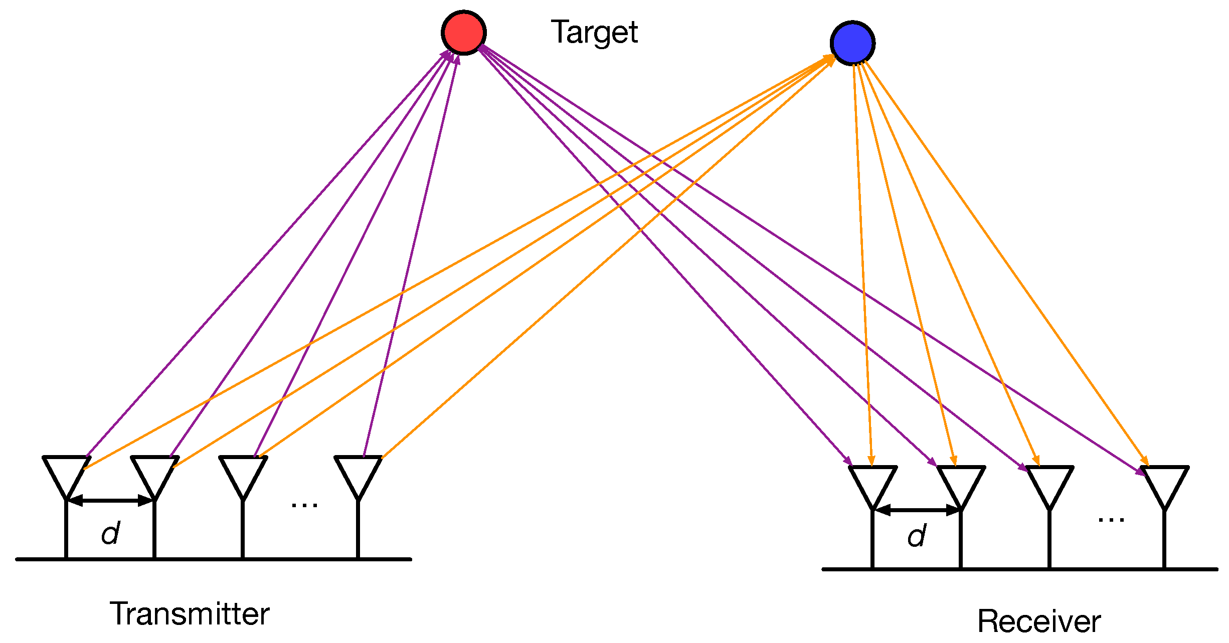
In this paper, the bistatic MIMO radar system [12,20,21] is considered and the radar system is shown in Figure 1, where M transmitting antennas and N receiving antennas are adopted. In each transmitting antenna, the orthogonal signal is transmitted. The transmitted waveform for the m-th transmitting antenna is denoted as () in the time domain, where p denotes the pulse index () and the number of pulses is P. Therefore, for the transmitted waveforms, we have
where denotes the pulse duration.

Figure 1.
The system model of the bistatic MIMO radar.
Assuming that there are K far-field targets, the direction of departure (DOD) and the direction of arrival (DOA) for the k-th target () are denoted as and , respectively. In each target, we assume that the the scattering coefficient is a type of Swerling II RCS [22] and follows the independent and identically distribution (i.i.d.) between pulses. Therefore, during the p-th pulse, the scattering coefficient of the k-th target can be denoted as .
Without considering the mutual coupling between antennas, the received signals in the n-th antenna () can be expressed as
where d denotes the fundamental antenna spacing, denotes the wavelength, and denotes the additive white Gaussian noise (AWGN) in the n-th receiving antenna during the p-th pulse, and .
After the matched filter for the m-th transmitted waveform and sampling at time , we can obtain the result of pulse compression
where we define , and . By collecting into a vector , the vector form of received signal can be obtained as
where the noise vector is defined as , and the steering vector in the transmitter is defined as
Collect all the received signals into a matrix, and we can obtain
where the steering vector in the receiver is defined as
and the noise matrix is defined as .
Vectorizing the matrix of received signals into a vector , the received signals can be expressed as the following vector form
where , and . Therefore, without the mutual coupling effect between antennas, the problem of DOD/DOA estimation is formulated in (8), where both and will be estimated from the received signal without the knowledge of target scattering coefficient .
2.2. Bistatic MIMO Radar System With Mutual Coupling
However, in the practical radar system, when the mutual coupling between the antennas in both transmitter and receiver is considered [23], the system model developed in (8) cannot be used. Therefore, this subsection will discuss the system model with mutual coupling. Usually, the mutual coupling matrices in the transmitter and receiver are respectively defined as [18]
where and denote the antenna impedance and terminating load in transmitter, and and denote the antenna impedance and terminating load in receiver. and denote the mutual impedance matrix in transmitter and receiver, respectively.
The -th row and -th column of mutual impedance matrix can be expressed as [19,24,25]
where , and L denotes the length of dipole antennas. and are defined respectively as
where denotes the distance between the -th antenna and the -th antenna. , , and are defined respectively as
and are defined respectively as
Similarly, the mutual impedance matrix can be also obtained from the expression of .
However, the expresses for and in (11) are too complex to analysis. Since and depend on the length of dipole antennas and the distances between antennas, the mutual coupling matrices and can be approximated, respectively, by two symmetric Toeplitz matrices
where is defined as
and is defined as
Additionally, for the mutual coupling matrices, we also have
Therefore, in the scenario with mutual coupling between antennas, the received signal in (8) can be rewritten as
where
The orthogonal signals are affected by the mutual coupling effect, but we describe the corresponding effect by a matrix, and the non-orthogonality is transferred into the steering vectors by the mutual coupling matrix.
Finally, collect the received signals from all pulses, and the matrix form of all received signals can be obtained as
where , . Then, the vector form of all received signals can be expressed as
where , .
Therefore, considering the mutual coupling between antennas in both receiver and transmitter, we will develop an algorithm to estimate the DOD/DOA in from the received signal in (29) without the knowledge of mutual coupling matrix and the scattering coefficient .
3. DOA/DOD and Mutual Coupling Matrix Estimation
With the received signal , we propose a novel sparse-based method to estimate the DOD/DOA in the scenario with unknown mutual coupling matrix. The possible DOD and DOA are, respectively, from the following two discretized sets
where and .
Therefore, assume that the DOD and DOA of a target are respectively the -th entry of , i.e., , and the -th entry of , i.e., , so the steering vector for this target can be expressed as
Then, collecting the steering vectors for all the possible targets, a dictionary matrix can be formulated as
Consequently, we can formulate the following compressed sensing (CS)-based problem [26,27] for the DOD/DOA estimation
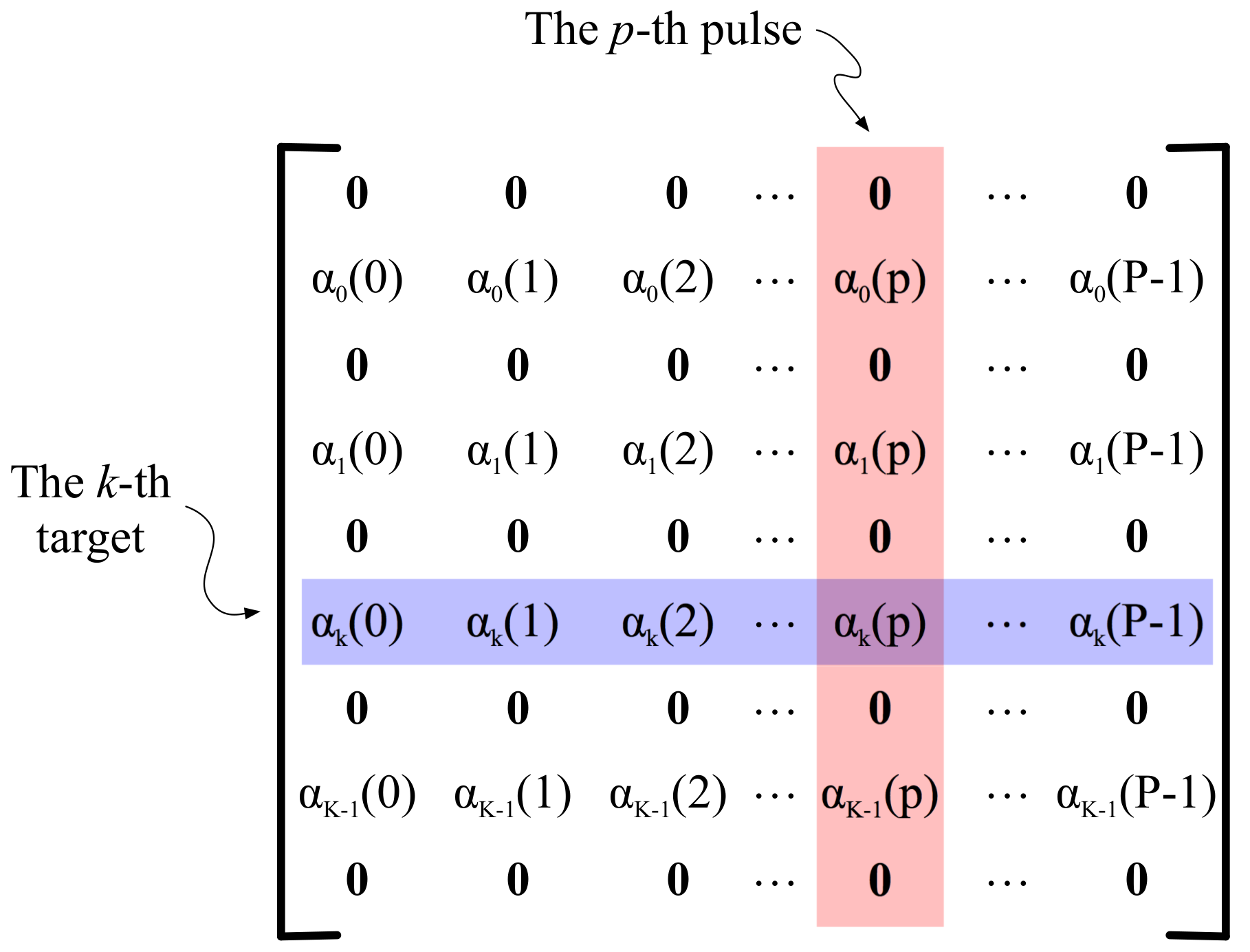
where the norm denotes the number of rows in with the nonzero entries, and the parameter is adopted to control the accuracy of sparse reconstruction. As shown in Figure 2, denotes a sparse matrix and the nonzero entries are the scattering coefficients from . The indexes of nonzero rows in indicate the DOD/DOA of targets.

Figure 2.
The structure of sparse matrix .
In (34), both the sparse matrix and the mutual coupling matrix are unknown, so this paper proposes a novel method to estimate DOD/DOA with the unknown mutual coupling matrix. Additionally, the off-grid problem in DOD/DOA estimation is also considered, where the off-grid problem means that the actual values of DOD/DOA can be not exactly contained by the discretized DOD and DOA sets, i.e., and , but and , for .
Unlike the traditional multiple measurement vectors (MMV) problem [28,29,30] in the CS theory, the mutual coupling matrix in the DOA/DOD estimation problem (34) is unknown, so the traditional MMV methods cannot be used directly. Therefore, a novel method is proposed to estimate DOD/DOA with the following objective function
where denotes the q-th row of , and
In (35), the norm is adopted as a relaxation form of norm [31].
A novel iterative method is proposed to solve the problem (35), and the flow chart of the proposed method is shown in Figure 3. First, ignoring the effect of mutual coupling, the CS-based method is adopted to estimate the sparse matrix with assuming . Second, based on the estimated , the mutual coupling matrix can be estimated as with the gradient descent method. Then, with the roughly estimated results, another gradient descent method is proposed to further polish the estimated results and solve the off-grid problem. Finally, Estimate DOD/DOA and mutual coupling matrix iteratively, and the estimated results are obtained when the estimation method is that of convergence. Details about the proposed method are given in the following subsections.
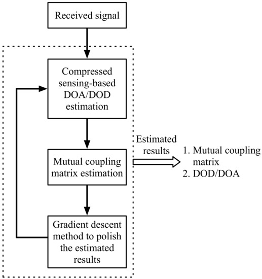
Figure 3.
The flow chart of proposed method for DOD/DOA estimation with the unknown mutual coupling matrix.
3.1. CS-Based DOD/DOA Estimation
The CS-based method is adopted to estimate DOD/DOA. Since the multiple pulses are adopted in the bistatic MIMO radar system, the simultaneous orthogonal matching pursuit (SOMP) method [32] can be adopted with ignoring the mutual coupling between antennas. In Algorithm 1, the details of the SOMP method for DOD/DOA estimation is given. At Step 4 of Algorithm 1, the norm is used to find the discretized DOD/DOA with the maximum correlation coefficient for all pulses.
| Algorithm 1 Simultaneous orthogonal matching pursuit for DOD/DOA estimation |
|
3.2. Gradient Decent-Based Mutual Coupling Matrix Estimation
With the estimated DOD/DOA and the sparse matrix , considering the symmetry characteristic of mutual coupling matrix, the mutual coupling vectors and can be estimated by the following objective function
where the objective function is defined as
Therefore, a gradient decent method is proposed in this paper to estimate the mutual coupling vectors and , and the details are given in Algorithm 2.
Here, the subgradients of objective function can be obtained as
where the subgradients of and are given respectively as
| Algorithm 2 Mutual coupling matrix estimation |
|
3.3. Polish the Estimated DOD/DOA and Mutual Coupling Matrix
The DOD/DOA are discretized and the dictionary matrix is formulated in Algorithm 1, so the estimated DOD/DOA must be in set and . However, in the practical scenarios, the DOD/DOA of targets are continuous and can be not exact in the sets with discretized angles. Therefore, with the roughly estimated DOD/DOA and mutual coupling matrix from Algorithms 1 and 2, this subsection proposes a gradient descent method to further polish the estimated results and solve the off-grid problem. The details to polish the estimation results is given in Algorithm 3. The mutual coupling effect is compensated in Algorithm 3, where we estimate the mutual coupling coefficients. Then, the estimated coefficients can be used to improve the performance of DOD/DOA estimation.
| Algorithm 3 Polish the estimated DOD/DOA and mutual coupling matrix |
|
The gradient descent method based on the subgradients of objective function , which are given in Proposition 1.
Theorem 1.
The subgradients ofare
where
- 1.
- The k-th column ofis
- 2.
- The k-th column ofis
- 3.
- The m-th column ofis
- 4.
- The n-th column ofis
- 5.
- The m-th entry ofis
- 6.
- The n-th entry ofis
Here, we will proof this proposition.
Proof.
The derivations for vectors or matrices are given in Appendix A. By defining , we can obtain
The k-th column of can be obtained as
where the m-th entry of is
Using the same method, can be also obtained. Additionally, we also have
and
where the k-th entry of is
so we have
Therefore, we can obtain
we can also obtain as
and the m-th column of is
Using the same method, can be also obtained. ☐
4. Cramér–Rao Lower Bound
The CRLB is adopted to show the lower bound on the variance of the estimated parameters including DOD/DOA ( and ), scattering coefficients (), and mutual coupling coefficients . CRLB can be obtained from the Fisher information matrix (FIM)
where is a vector with the diagonal entries of . can be calculated as
where
The subgradients of are calculated as follows:
- is obtained aswhere the k-th column of isandWith the same method, we can obtain .
- is obtained asand we have .
- is obtained aswhere the n-th column of is
- is obtained aswhere the n-th column of is
Finally, the FIM is obtained as
where , , , . Then, with FIM, the corresponding CRLB can be obtained.
5. Computational Complexity
In Algorithm 1, to estimate the DOD/DOA using the SOMP method, the computational complexity is . In Algorithm 2 to estimate the mutual coupling matrix, the computational complexity is . Additionally, in Algorithm 3, the estimation results are polished, and the computational complexity is . Therefore, the computational complexity of the proposed method to estimate DOD/DOA and the mutual coupling matrix can be roughly expressed as . Usually, we have , so the roughly computational complexity can be simplified as .
6. Simulation Results
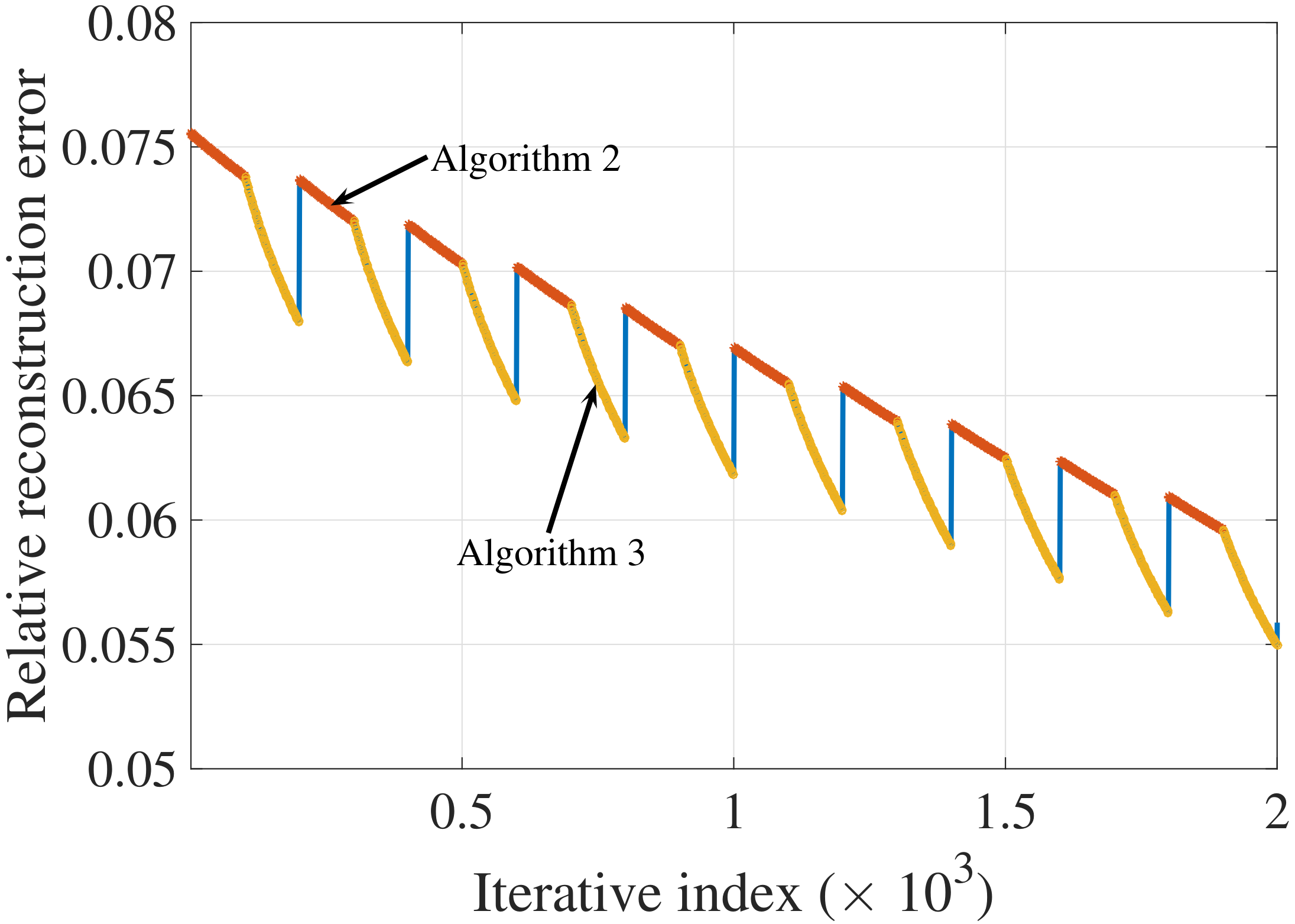
In this section, the simulation results are given to show the performance of the proposed algorithm. The simulation parameters are given in Table 1. First, the reconstruction performance for the received signal is shown in Figure 4. The reconstruction error is defined as
where is the received signal defined in (29), and is the reconstruction signal with the estimated parameters including DOD/DOA, scattering coefficients and mutual coupling matrices. As shown in Figure 4, the proposed method polishes the estimated DOD/DOA and mutual coupling matrices iteratively, where Algorithm 2 is adopted to estimate mutual coupling matrices and Algorithm 3 is used to polished the estimated DOD/DOA and mutual coupling matrices. The relative reconstruction error is decreasing with increasing the number of iterations. Additionally, as shown in this figure, Algorithm 3 is more significant in improving the estimation performance than Algorithm 2. Therefore, it is efficient to polish the estimated results in the off-grid problem after the rough on-grid estimation.

Table 1.
Simulation parameters.

Figure 4.
The reconstruction performance with the proposed Algorithms 2 and 3.
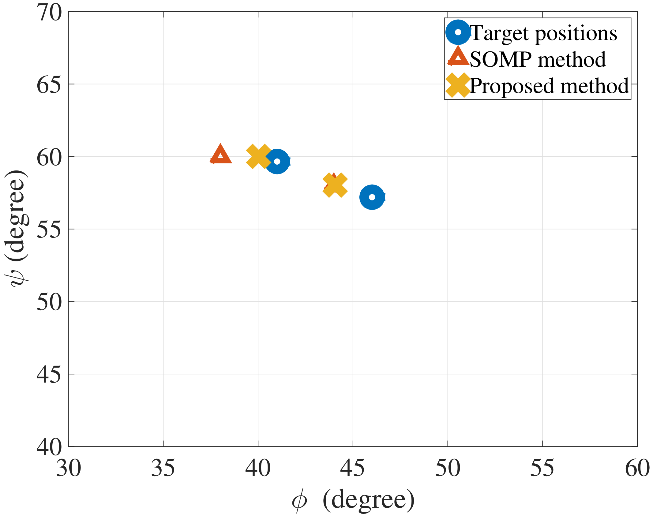
Figure 5 shows the estimated DOD/DOA using different methods, where ◯ denotes the DOD/DOA of the target, × denotes the estimated DOD/DOA with the proposed method, and △ denotes the estimated DOD/DOA with the on-grid SOMP method [32]. As shown in this figure, when only the on-grid SOMP method is used to estimate the target DOD/DOA, the estimation error is larger than that using the proposed method. In the proposed method, we adopt the proposed off-grid method to further improve the on-grid result, so the proposed method can outperform the traditional on-grid method.
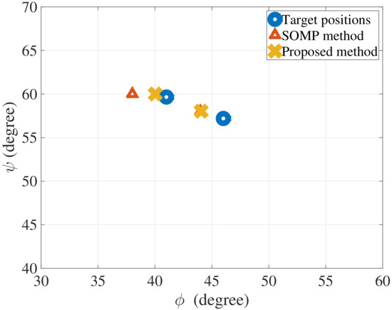
Figure 5.
The estimated DOD/DOA using different methods.
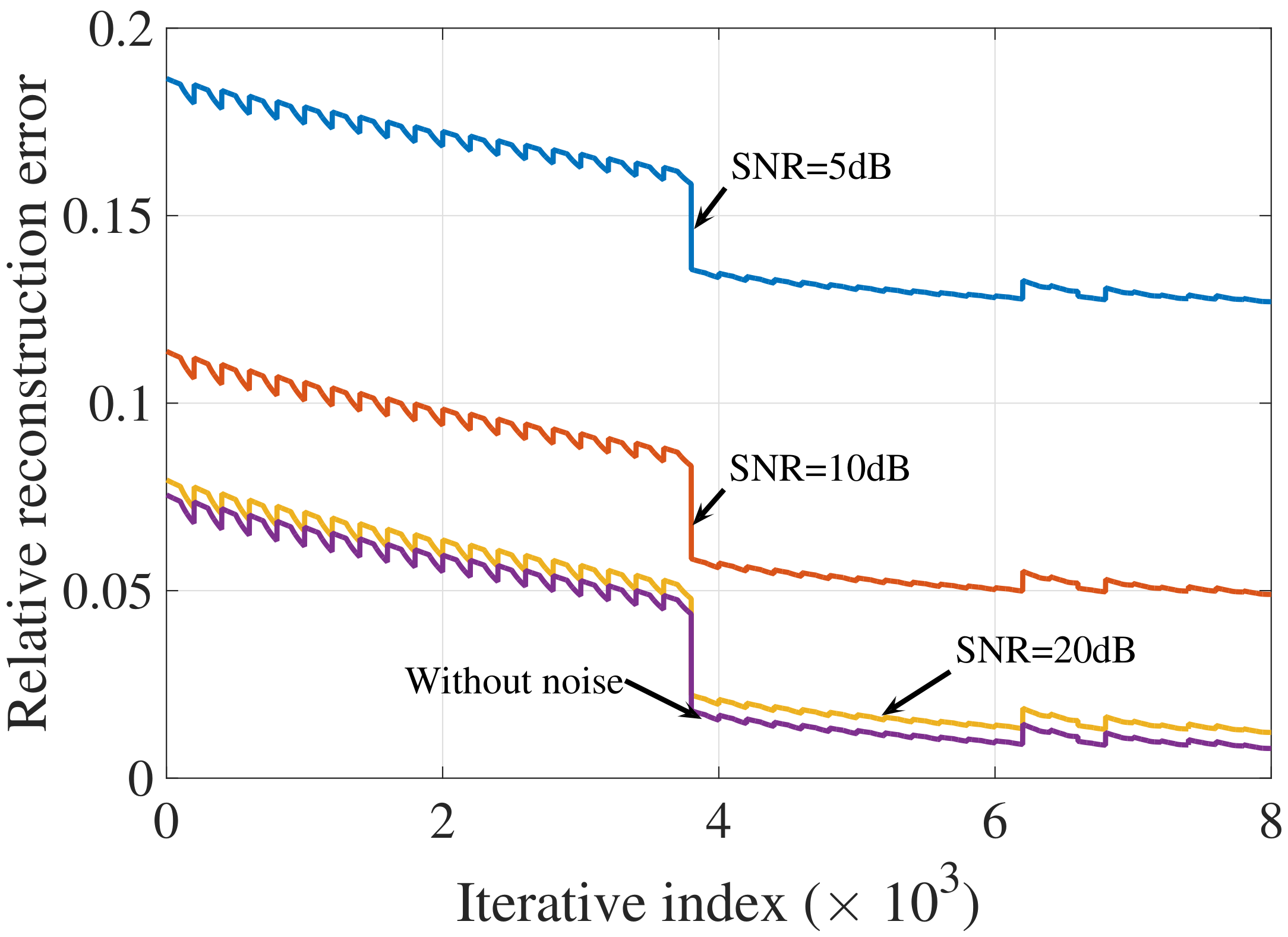
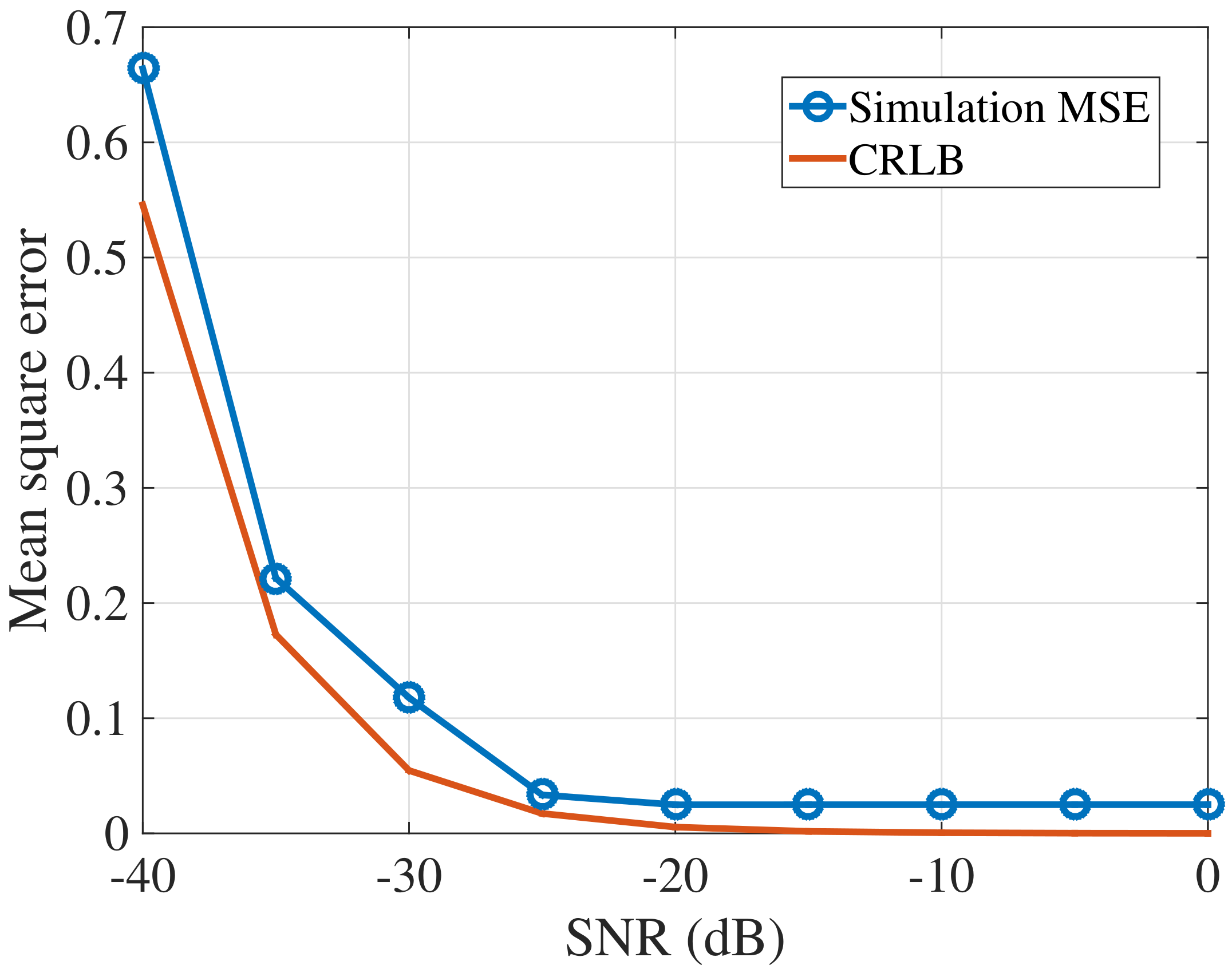
Figure 6 shows the reconstruction performance with the proposed method where the signal-to-noise ratios (SNRs) are 5 dB, 10 dB and 20 dB. With different SNRs, the same waveforms are adopted, so the correlation between waveforms are the same. As shown in this figure, with increasing the SNR of the received signal, better reconstruction performance can be achieved. Additional, when SNR = 20 dB, the reconstruction performance is almost the same as the one without noise. After about iterations, the reconstruction performance is convergence, so we can adopt as the maximum number of iterations in the following simulations. In Figure 7, we also compare the estimated results with the CRLB derived in this paper. As shown in this figure, the proposed estimation method can approach the CRLB, so the estimation method is efficient.

Figure 6.
The iterative results for different SNRs.

Figure 7.
The CRLB and the simulation MSE of the proposed method.
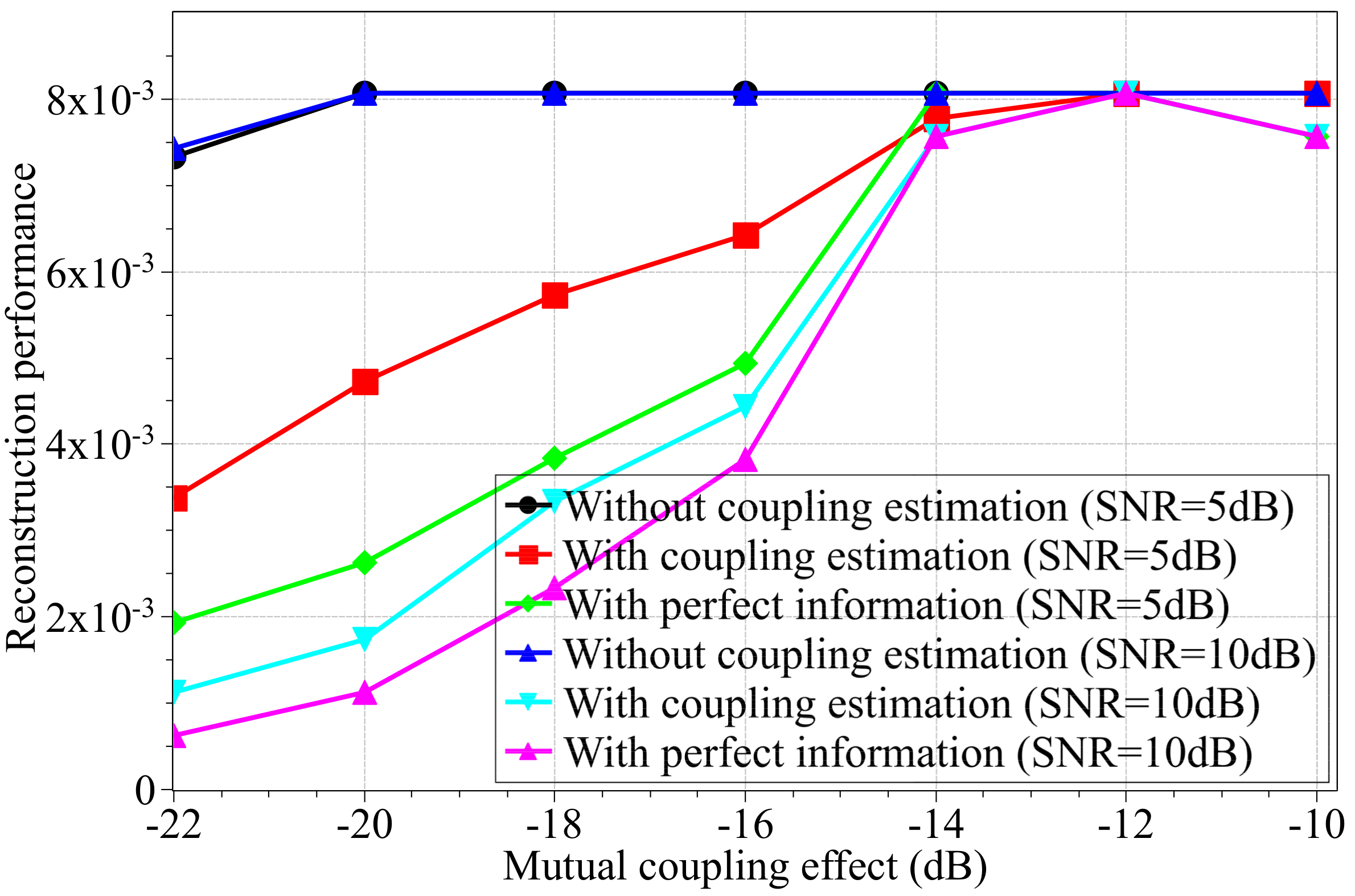
In Figure 8, we show the effect of mutual coupling on the estimation performance. As shown in this figure, better estimation performance can be achieved by improving the SNR of the received signal. The curves “with perfect information” are the simulation results with the perfect information of mutual coupling effect. The best estimation performance can be achieved by the methods with perfect information. Moreover, the mutual coupling has great effect on the estimation performance, so better reconstruction performance can be achieved by estimating the mutual coupling matrices during the DOD/DOA estimation. With different target numbers, Figure 9 shows the reconstruction estimation performance. The targets are uniformly distributed in the angle range from 30 to 60. When the target number is increasing, the reconstruction performance will be worse with the high correlation between the echoed waveforms from different targets. However, with better SNR, more targets can be estimated with the same reconstruction performance.
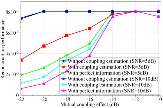
Figure 8.
The reconstruction performance with and without coupling estimation.
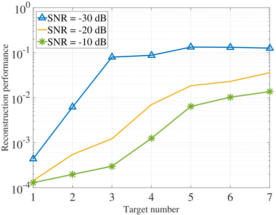
Figure 9.
The reconstruction performance with different numbers of targets.
7. Conclusions
In the bistatic MIMO radar, the DOD/DOA estimation problem with mutual coupling effect between antennas has been addressed. After formulating the system model, the iterative method based on CS has been proposed to exploit the sparsity of targets in the detection area, where the estimation for DOD/DOA and mutual coupling has been polished by solving the off-grid problem. Then, the corresponding CRLBs for the parameters including DOD/DOA, mutual coupling matrices, and scattering coefficients, have been derived. Simulation results show that the proposed estimation method can approach the CRLB and achieve the better estimation performance than the traditional methods. Further work will focus on the estimation of moving targets in the MIMO radar system with mutual coupling.
Author Contributions
Conceptualization, P.C. and Z.C. (Zhenxin Cao); methodology, P.C.; software, Z.C. (Zhimin Chen); validation, C.Y.; formal analysis, Z.C. (Zhimin Chen); investigation, Z.C. (Zhimin Chen); resources, P.C.; data curation, Z.C. (Zhenxin Cao); writing—original draft preparation, P.C.; writing—review and editing, P.C.; visualization, Z.C. (Zhimin Chen); supervision, Z.C. (Zhenxin Cao); project administration, P.C.; funding acquisition, P.C.
Funding
This work was supported in part by the National Natural Science Foundation of China (Grant No. 61801112, 61471117, 61601281), the Natural Science Foundation of Jiangsu Province (Grant No. BK20180357), the Open Program of State Key Laboratory of Millimeter Waves (Southeast University, Grant No. Z201804).
Conflicts of Interest
The authors declare no conflict of interest.
Appendix A. The Derivations of Complex Vector and Matrix
Lemma A1.
With both the complex vectors (, ) and the complex matrixbeing the function of a complex vector, the following derivations can be obtained [33]
Proof.
With and being the function of , we can obtain the entry in m-th row and n-th column of as
so the n-th column of is
and
☐
References
- Li, J.; Stoica, P. MIMO radar with colocated antennas. IEEE Signal Process. Mag. 2007, 24, 106–114. [Google Scholar] [CrossRef]
- Haimovich, A.M.; Blum, R.S.; Cimini, L.J. MIMO radar with widely separated antennas. IEEE Signal Process. Mag. 2007, 25, 116–129. [Google Scholar] [CrossRef]
- Fishler, E.; Haimovich, A.; Blum, R.; Chizhik, D.; Cimini, L.; Valenzuela, R. MIMO radar: An idea whose time has come. In Proceedings of the IEEE Radar Conference, Philadelphia, PA, USA, 26–29 April 2004; pp. 71–78. [Google Scholar]
- Chen, P.; Qi, C.; Wu, L.; Wang, X. Estimation of Extended Targets Based on Compressed Sensing in Cognitive Radar System. IEEE Trans. Veh. Technol. 2017, 66, 941–951. [Google Scholar] [CrossRef]
- Fishler, E.; Haimovich, A.; Blum, R.S.; Cimini, L.J.; Chizhik, D.; Valenzuela, R.A. Spatial diversity in radars-models and detection performance. IEEE Trans. Signal Process. 2006, 54, 823–838. [Google Scholar] [CrossRef]
- Davis, M.; Showman, G.; Lanterman, A. Coherent MIMO radar: The phased array and orthogonal waveforms. IEEE Aerosp. Electron. Syst. Mag. 2014, 29, 76–91. [Google Scholar] [CrossRef]
- Chen, P.; Wu, L.; Qi, C. Waveform Optimization for Target Scattering Coefficients Estimation Under Detection and Peak-to-Average Power Ratio Constraints in Cognitive Radar. Circ. Syst. Signal Process. 2016, 35, 163–184. [Google Scholar] [CrossRef]
- Chen, P.; Qi, C.; Wu, L. Antenna placement optimisation for compressed sensing-based distributed MIMO radar. IET Radar Sonar Navig. 2017, 11, 285–293. [Google Scholar] [CrossRef]
- Willis, N.J.; Griffiths, H.D. Advances in Bistatic Radar; Institution of Engineering and Technology: Stevenage, UK, 2007. [Google Scholar]
- Zhang, J.; Wang, H.; Zhu, X. Adaptive waveform design for separated transmit/receive ULA-MIMO radar. IEEE Trans. Signal Process. 2010, 58, 4936–4942. [Google Scholar] [CrossRef]
- Yao, B.; Wang, W.; Yin, Q. DOD and DOA estimation in bistatic non-uniform multiple-input multiple-output radar systems. IEEE Commun. Lett. 2012, 16, 1796–1799. [Google Scholar] [CrossRef]
- Jiang, H.; Zhang, J.K.; Wong, K.M. Joint DOD and DOA estimation for bistatic MIMO radar in unknown correlated noise. IEEE Trans. Veh. Technol. 2015, 64, 5113–5125. [Google Scholar] [CrossRef]
- Chen, P.; Qi, C.; Wu, L.; Wang, X. Waveform Design for Kalman Filter-Based Target Scattering Coefficient Estimation in Adaptive Radar System. IEEE Trans. Veh. Technol. 2018. [Google Scholar] [CrossRef]
- Zhang, X.; Xu, L.; Xu, L.; Xu, D. Direction of departure (DOD) and direction of arrival (DOA) estimation in MIMO radar with reduced-dimension MUSIC. IEEE Commun. Lett. 2010, 14, 1161–1163. [Google Scholar] [CrossRef]
- Bencheikh, M.L.; Wang, Y. Joint DOD-DOA estimation using combined ESPRIT-MUSIC approach in MIMO radar. Electron. Lett. 2010, 46, 1796–1799. [Google Scholar] [CrossRef]
- Zheng, G.; Tang, J.; Yang, X. ESPRIT and unitary ESPRIT algorithms for coexistence of circular and noncircular signals in bistatic MIMO radar. IEEE Access 2016, 4, 7232–7240. [Google Scholar] [CrossRef]
- Oh, D.; Li, Y.C.; Khodjaev, J.; Chong, J.W.; Lee, J.H. Joint estimation of direction of departure and direction of arrival for multiple-input multiple-output radar based on improved joint ESPRIT method. IET Radar Sonar Navig. 2015, 9, 308–317. [Google Scholar] [CrossRef]
- Zhang, C.; Huang, H.; Liao, B. Direction finding in MIMO radar with unknown mutual coupling. IEEE Access 2017, 5, 4439–4447. [Google Scholar] [CrossRef]
- Zheng, Z.; Zhang, J.; Zhang, J. Joint DOD and DOA estimation of bistatic MIMO radar in the presence of unknown mutual coupling. Signal Process. 2012, 92, 3039–3048. [Google Scholar] [CrossRef]
- Chen, P.; Zheng, L.; Wang, X.; Li, H.; Wu, L. Moving target detection using colocated MIMO radar on multiple distributed moving platforms. IEEE Trans. Signal Process. 2017, 65, 4670–4683. [Google Scholar] [CrossRef]
- Liu, X.L.; Liao, G.S. Multi-target localisation in bistatic MIMO radar. Electron. Lett. 2010, 46, 945–946. [Google Scholar] [CrossRef]
- Skolnik, M. Radar Handbook, 3rd ed.; McGraw-Hill: New York, NY, USA, 2008. [Google Scholar]
- Maio, A.D.; Landi, L.; Farina, A. Adaptive radar detection in the presence of mutual coupling and near-field effects. IET Radar Sonar Navig. 2008, 2, 17–24. [Google Scholar] [CrossRef]
- Lin, M.; Yang, L. Blind calibration and DOA estimation with uniform circular arrays in the presence of mutual coupling. IEEE Antennas Wirel. Propag. Lett. 2006, 5, 315–318. [Google Scholar] [CrossRef]
- Liu, C.L.; Vaidyanathan, P.P. Super nested arrays: Linear sparse arrays with reduced mutual coupling—Part I: Fundamentals. IEEE Trans. Signal Process. 2016, 64, 3997–4012. [Google Scholar] [CrossRef]
- Candes, E.J.; Wakin, M.B. An introduction to compressive sampling. IEEE Signal Process. Mag. 2008, 25, 21–30. [Google Scholar] [CrossRef]
- Donoho, D.L. Compressed sensing. IEEE Trans. Inf. Theory 2006, 52, 1289–1306. [Google Scholar] [CrossRef]
- Li, Y.; Chi, Y. Off-the-grid line spectrum denoising and estimation with multiple measurement vectors. IEEE Trans. Signal Process. 2016, 64, 1257–1269. [Google Scholar] [CrossRef]
- Choi, J.W.; Shim, B. Statistical recovery of simultaneously sparse time-varying signals from multiple measurement vectors. IEEE Trans. Signal Process. 2015, 22, 6136–6148. [Google Scholar] [CrossRef]
- Jin, Y.; Rao, B.D. Support recovery of sparse signals in the presence of multiple measurement vectors. IEEE Trans. Inf. Theory 2013, 59, 3139–3157. [Google Scholar] [CrossRef]
- Zheng, L.; Maleki, A.; Weng, H.; Wang, X.; Long, T. Does ℓp-minimization outperform ℓ1-minimization? IEEE Trans. Inf. Theory 2017, 63, 6896–6935. [Google Scholar] [CrossRef]
- Determe, J.F.; Louveaux, J.; Jacques, L.; Horlin, F. On the noise robustness of simultaneous orthogonal matching pursuit. IEEE Trans. Signal Process. 2017, 65, 864–875. [Google Scholar] [CrossRef]
- Petersen, K.B.; Pedersen, M.S. The Matrix Cookbook; Technical University of Denmark: Lyngby, Denmark, 2008; Volume 7, p. 15. [Google Scholar]


© 2018 by the authors. Licensee MDPI, Basel, Switzerland. This article is an open access article distributed under the terms and conditions of the Creative Commons Attribution (CC BY) license (http://creativecommons.org/licenses/by/4.0/).