Event-Triggered Containment Control of Multi-Agent Systems With High-Order Dynamics and Input Delay

Abstract

This paper studies the problem of distributed containment control for multi-agent systems with high-order dynamics and input delays. Two event-triggered control algorithms are proposed for multi-agent systems without and with input delay, respectively. The communication instants between two linked followers are determined by the event-triggering condition, and every follower can detect the event based on its own control input. For the followers, edge-based estimators are adopted to predict state differences to neighbors. Control inputs of the followers are calculated based on the predicted values of the state differences. To deal with the input delay, a delay comprehension approach is developed. It is proved that for arbitrarily large but bounded input delays, the followers can move into the convex hull spanned by the leaders asymptotically. Simulation results show the effectiveness of the proposed algorithms.

1. Introduction

Distributed cooperative control of multi-agent systems has been studied extensively in the past decade. Compared with its centralized counterpart, distributed control has many advantages such as low cost, easy maintenance, and high adaptivity. As a fundamental problem in distributed cooperative control, the consensus problem has attracted much attention. For a group of agents, consensus means reaching an agreement on a quantity of interest. The consensus problem can be classified into leaderless consensus and leader-following consensus, according to the absence or presence of a leader. Recently, much progress has been made on both leaderless and leader-following consensus problems (see [1,2,3,4,5] and references therein).

Although the leader-following consensus problem for multi-agent systems with single leader is interesting, it is sometimes more meaningful to study the leader-following problem for multi-agent systems with multiple leaders. This problem is called the containment problem, the objective of which is to steer all the followers into the convex hull spanned by the leaders. In recent years, researchers have paid much attention to the containment control problem owing to its wide applications in swarm robotics [6,7,8,9,10,11,12,13,14,15,16]. In [17], the containment control problem is investigated in both continuous-time and discrete-time domain. A $P{I}^n$-Type containment control algorithm is proposed, which allows the followers to be of any-order integral dynamics.

In the aforementioned results, it is assumed that the agents can access their neighbors’ states continuously or with a fixed frequency. This is unnecessary or unrealistic in many applications. On one hand, it is a waste of communication resource to access the neighbors’ states frequently when the system states nearly approach their equilibriums or there are no disturbances imposed on the system [18,19,20]. On the other hand, too much communication may lead to rising power costs and network congestion, which may degrade the performance of the system [21,22,23]. The event-triggered control is a good strategy to solve this problem [24,25,26]. Compared with the traditional sampled-data-based control, where the measurement or control is triggered by time, the main feature of the event-triggered control is that the measurement or control action is triggered by an event condition. The event-triggered control strategy was applied in both leaderless and leader-following consensus problems for multi-agent systems in [27,28,29]. For more details, one can refer to [30] and references therein. More recently, the authors in [31,32,33] have proposed some event-triggered containment control algorithms for multi-agent systems with multiple leaders.

Time-delay exists in most practical systems. So, it is very meaningful to investigate the stability of time-delay systems [34,35,36,37,38,39,40]. For multi-agent systems, the effect of time-delay is also an important problem to be considered. There are two sources of time-delay in multi-agent systems. One source is the communication among agents, which is called communication delays. The other source is the processing time for the information arrived at each agent, which is called input delays. The consensus problem for multi-agent system with communication/input delays has been extensively investigated in the literature (see [41] and references therein). For second-order multi-agent systems with time-varying delays, the containment control problem is considered in [42]. Recently, Miao et al. addressed the containment problem for second-order multi-agent systems with constant input delays [43]. An event-triggered containment control algorithm was proposed, together with conditions under which the followers will converge to the convex hull spanned by the leaders.

In this paper, we consider the event-triggered containment control problem for multi-agent systems with high-order dynamics and input delay. Motivated by [29], model-based approach is developed to avoid continuous communications among followers, and edge-based estimators are designed to predict state differences to neighbors. New event-triggered containment control algorithms are proposed for multi-agent systems without and with input delay, respectively. Sufficient conditions are derived under which the followers will move into the convex hull formed by the leaders. Compared with existing literatures on the containment control problem for multi-agent systems, our contribution is summarized as follows.

• A delay compensation-based event-triggered containment controller is developed. It is proved that for arbitrarily large but bounded constant input delays, the proposed controller can drive all the followers into the convex hull formed by the leaders. In contrast, the controller in [43] can deal with input delays below an upper bound only.
• The proposed algorithms are distributed, while the algorithms in [31,32,33,43] are centralized. Using the algorithms proposed in this paper, every follower can decide whether the event should be triggered based on its own control input. However, using algorithms in [31,32,33,43], all agents need their neighbors’ states to trigger the next communication.
• Compared with the containment control algorithms with continuous [6,7,8,9,10,11,12,13,14,15,16] or periodic communications [17], the proposed event-triggered containment control algorithms has the potential to reduce the communication burden of multi-agent systems.

Notations: Throughout this paper, ${\mathbb{R}}^l$ denotes the l dimensional Euclidean space, $0_{p\times q}$ denotes a $p\times q$ matrix with all the elements to be zero. Given a vector $\mu$, $\parallel \mu \parallel$ denotes the Euclidean norm of $\mu$. Given a matrix A, $A>0$ means that A is a positive definite matrix, $\parallel A\parallel$ is the induced norm of A. The superscript T denotes the transpose of a vector or matrix. We use $\mathrm{diag}({\mu }_1,\cdots ,{\mu }_p)$ to denotes the diagonal matrix of all ${\mu }_1$, ⋯, ${\mu }_p$.

2. Problem Formulation

2.1. Algebraic Graph Theory

Consider a group of agents consisted of M leaders and N followers. The leaders do not need to access information from the followers, while the followers are guided by the leaders. We assume that only a part of the followers can access information from some leaders. These followers are called informed followers. The rest of the followers cannot receive information from the leaders directly.

We use graph $\mathcal{G}=(\mathcal{V},\mathcal{E})$ to denote the communication topology among the leaders and the followers, where $\mathcal{V}=\{1,\cdots ,M+N\}$ is the node set and $\mathcal{E}\subseteq \mathcal{V}\times \mathcal{V}$ is the edge set. A directed edge $(j,i)\in \mathcal{E}$ denotes that node i can receive information from node j but not necessarily vice versa. An undirected edge $(j,i)\in \mathcal{E}$ denotes that node i and node j can access information from each other. A graph is undirected if all the edges in the graph are undirected. The neighbor set ${\mathcal{N}}_i=\{j\mid (j,i)\in \mathcal{E}\}$ denotes the set of nodes from which node i can access information. A directed path is a sequence of directed edges of the form $(i_1,i_2)$, $(i_2,i_3)$,..., where $i_j\in \mathcal{V}$.

The adjacency matrix ${\mathcal{A}}_d=[a_{ij}]\in {\mathbb{R}}^{(M+N)\times (M+N)}$ is defined as $a_{ij}>0$ if $(j,i)\in \mathcal{E}$ and $a_{ij}=0$ otherwise. The Laplacian matrix $L=[l_{ij}]\in {\mathbb{R}}^{(M+N)\times (M+N)}$ is defined as $l_{ii}={\sum }_{j=1,j\ne i}^{M+N}{a}_{ij}$ and $l_{ij}=-a_{ij}$, $i\ne j$. We use $\mathcal{L}=\{1,2,\cdots ,M\}$ and $\mathcal{F}=\{M+1,M+2,\cdots ,M+N\}$ to denote node set of the leaders and the followers, respectively. Notice that $a_{ij}=0$ for all $i=1,\cdots ,M$ and $j=1,\cdots ,M+N$, because the leaders have no neighbors. Therefore, the Laplacian matrix L can be rewritten as

$$\begin{array}{c}\hfill L=\left[\begin{array}{cc}{0}_{M\times M}& 0_{M\times N}\\ L_1& L_2\end{array}\right].\end{array}$$

(1)

In this paper, for the sake of convenience, we assume that $a_{ij}=1$, if $(j,i)\in \mathcal{E}$.

2.2. System Models and Control Objectives

Consider a network of M leaders and N followers with the following linear dynamics:

$$\begin{array}{ccc}\hfill {\dot{x}}_i(t)& =& A{x}_i(t),i\in \mathcal{L},\hfill \end{array}$$

(2)

$$\begin{array}{ccc}\hfill {\dot{x}}_i(t)& =& A{x}_i(t)+B{u}_i(t),i\in \mathcal{F},\hfill \end{array}$$

(3)

where $x_i(t)\in {\mathbb{R}}^n$ and $u_i(t)\in {\mathbb{R}}^m$ are the state and the control input of agent i, respectively; A and B are constant matrices with appropriate dimensions.

When there exists a constant input delay $\tau$, (3) becomes

$$\begin{array}{c}\hfill {\dot{x}}_i(t)=A{x}_i(t)+B{u}_i(t-\tau ),i\in \mathcal{F}.\end{array}$$

(4)

Definition 1.

Let $\mathcal{C}={\mathbb{R}}^p$. The set $\mathcal{C}$ is said to be convex if for any x and y in $\mathcal{C}$, the point $(1-\alpha )x+\alpha y$ is in $\mathcal{C}$ for any $\alpha \in [0,1]$. The convex hull $\mathrm{Co}(X)$ of a set of points $X=\{x_1,\cdots ,x_q\}$ is the minimal convex set containing all points in X.

Definition 2.

We say algorithm $u_i(t)$ asymptotically solves the containment problem if, under algorithm $u_i(t)$, the followers move into the convex hull formed by the leaders asymptotically.

The following assumptions and lemmas are used later.

Assumption 1.

The communication graph among the followers is undirected. For each follower, there exists at least one leader that has a path to it.

Lemma 1

([13]).Under assumption 1, the matrix $L_2$ defined in (1) is symmetric positive definite.

From Lemma 1 we have all the eigenvalues of $L_2$ are positive. Assume that the eigenvalues of $L_2$ are ${\lambda }_1\le {\lambda }_2\cdots \le {\lambda }_N$.

Lemma 2.

Each entry of $-L_2^{-1}{L}_1$ is nonnegative and each row sum of $-L_2^{-1}{L}_1$ is equal to one.

Lemma 3.

Assume that the matrix pair $(A,B)$ is controllable, and all the poles of A are on the imaginary axis. For any constant scalar $\gamma >0$, the parametric Riccati equation

$$\begin{array}{c}\hfill A^{T}P+PA-PB{B}^{T}P=-\gamma P\end{array}$$

(5)

has a unique positive definite matrix $P(\gamma )=W^{-1}(\gamma )$, where $W(\gamma )$ is the unique positive definite solution to the following Lyapunov equation $W{(A+\frac{\gamma }{2}{I}_n)}^T+(A+\frac{\gamma }{2}{I}_n)W=B{B}^T$. Moreover, ${lim}_{\gamma \to 0^{+}}P(\gamma )=0$, $\frac{d}{d\gamma }P(\gamma )>0$, $\forall \gamma >0$, $tr(B^{T}P(\gamma )B)=n\gamma$, $P(\gamma )B{B}^{T}P(\gamma )\le n\gamma P(\gamma )$, $e^{At}P(\gamma )e^{At}\le e^{(n-1)\gamma t}P(\gamma )$. Moreover, if all the eigenvalues of A are zero, then $A^{T}P(\gamma )A\le 3{(n\gamma )}^{2}P(\gamma )$.

2.3. Event-Triggered Communication Mechanisms

As will be explained later, since control inputs of the leaders are zero, the informed followers can estimate states of the leaders based on their initial states. Therefore, the event-triggered mechanism is not needed for the communication between the leaders and the informed followers.

Assume that followers i and j are two linked agents, and they exchange information at event instants $\{t_{ij}^0,t_{ij}^1\dots ,t_{ij}^k\dots \}$. To exchange information based on the event-triggering communication mechanism, event trigging functions $f_{ij}(t)$ and $f_{ji}(t)$ should be designed for each edge $(j,i)$. The event instants between followers i and j are determined according to

$$\begin{array}{c}\hfill t_{ij}^{k+1}=t_{ji}^{k+1}=inf\{t\mid t>t_{ij}^k,f_{ij}(t)\le 0or{f}_{ji}(t)\le 0\},j\in {\mathcal{N}}_i\end{array}$$

(6)

where $t_{ij}^0=t_{ji}^0=0$. Once $f_{ij}(t)$ reaches zero, an event is triggered. Follower i will send $x_i(t)$ to follower j, and then receive $x_j(t)$ from follower j. Conversely, if $f_{ji}(t)$ reach zero first, follower j will send $x_j(t)$ to follower i, and then receive $x_i(t)$ from follower i.

The objective of this paper is to design the event-triggering functions and the control algorithms for system (2) and (3) without input delay, and the input delay system (2) and (4), respectively, such that all the followers can move to the convex hull formed by the leaders.

3. Event-Triggered Containment Control without Input Delay

In this section, we consider the containment control problem without input delay. Define $x_{\mathcal{F}}(t)={\left[\begin{array}{ccc}{x}_{M+1}^T(t),& \cdots ,& x_{M+N}^T(t)\end{array}\right]}^T$, and $x_{\mathcal{L}}(t)={\left[\begin{array}{ccc}{x}_1^T(t),& \cdots ,& x_M^T(t)\end{array}\right]}^T$. Note from Lemma 2 that if

$$\begin{array}{c}\hfill x_{\mathcal{F}}(t)=-(L_2^{-1}{L}_1\otimes I_n)x_{\mathcal{L}}(t),\end{array}$$

(7)

then all the followers are in the convex hull formed by the leaders. For follower i, define

$$\begin{array}{c}\hfill {\phi }_i(t)=\sum _{j\in \mathcal{L}\cup \mathcal{F}}{a}_{ij}[x_i(t)-x_j(t)].\end{array}$$

(8)

If ${\phi }_i(t)=0$ for $i=M+1,\dots ,M+N$, one has

$$\begin{array}{c}\hfill (L_2\otimes I_n)x_{\mathcal{F}}(t)+(L_1\otimes I_n)x_{\mathcal{L}}(t)=0,\end{array}$$

(9)

which implies that (7) holds. Therefore, all the followers lie in the convex hull formed by the leaders if ${\phi }_i(t)=0$ holds for $i=M+1,\dots ,M+N$.

Let $e_{ij}(t)=x_i(t)-x_j(t)$ be the state difference between follower i and leader j, and $z_{ij}(t)=x_i(t)-x_j(t)$ be the state difference between followers i and j. Equation (8) can be rewritten as

$$\begin{array}{c}\hfill {\phi }_i(t)=\sum _{j\in \mathcal{L}}{a}_{ij}{e}_{ij}(t)+\sum _{j\in \mathcal{F}}{a}_{ij}{z}_{ij}(t),i=M+1,\dots ,M+N.\end{array}$$

(10)

For informed followers, to drive ${\phi }_i(t)$ to zero, $e_{ij}(t)$ and $z_{ij}(t)$ are needed. For other followers, $z_{ij}(t)$ is needed. However, when the event-triggering communication mechanism is adopted, such information is available only at the event instants. To solve this problem, we need the following state difference estimators to estimate $e_{ij}(t)$ and $z_{ij}(t)$ during the inter-event intervals.

3.1. Leader Edge State Difference Estimators

Suppose that informed follower i can access leader j’s state. In this case, edge $(j,i)$ is called leader edge of follower i. From (2) and (3) and the definition of $e_{ij}(t)$ we have

$$\begin{array}{c}\hfill {\dot{e}}_{ij}(t)=A{e}_{ij}(t)+B{u}_i(t).\end{array}$$

(11)

Follower i can construct the following estimator to estimate $e_{ij}(t)$

$$\begin{array}{c}\hfill {\dot{\widehat{e}}}_{ij}(t)=A{\widehat{e}}_{ij}(t)+B{u}_i(t),\end{array}$$

(12)

where ${\widehat{e}}_{ij}(0)=e_{ij}(0)=x_i(0)-x_j(0)$. The solution of (12) is

$$\begin{array}{c}\hfill e_{ij}(t)=e^{At}{e}_{ij}(0)+{\int }_0^t{e}^{A(t-s)}B{u}_i(s)ds.\end{array}$$

(13)

Remark 1.

It is trivial to prove that ${\widehat{e}}_{ij}(t)=e_{ij}(t)$, for all $t>0$. So, the informed followers can estimate $e_{ij}(t)$ based on the initial state $x_j(0)$, i.e., they only need to communicate with the leaders one time. This is because the leaders’ control inputs are assumed to be zero. If the leaders’ control inputs are nonzero, the informed followers need to communicate with their leader neighbors frequently. Tracking dynamic leaders with an event-triggered controller is a tough problem, which will be considered in our future work.

3.2. Neighbor Edge State Difference Estimators

Suppose that follower i can access follower j’s state. In this case, edge $(j,i)$ is called neighbor edge of follower i. From (3) we have

$$\begin{array}{c}\hfill {\dot{z}}_{ij}(t)=A{z}_{ij}(t)+B[u_i(t)-u_j(t)].\end{array}$$

(14)

In the inter-event interval $(t_{ij}^k,t_{ij}^{k+1})$, $u_j(t)$ is not available for follower i. Follower i can adopt the following estimator to estimate $z_{ij}(t)$

$$\begin{array}{c}\hfill {\dot{\widehat{z}}}_{ij}(t)=A{\widehat{z}}_{ij}(t),\end{array}$$

(15)

where ${\widehat{z}}_{ij}(0)=z_{ij}(0)$ and ${\widehat{z}}_{ij}(t_{ij}^k)=z_{ij}(t_{ij}^k)$. The solution of (15) in inter-event interval $(t_{ij}^k,t_{ij}^{k+1})$ is

$$\begin{array}{c}\hfill {\widehat{z}}_{ij}(t)=e^{A(t-t_{ij}^k)}{z}_{ij}(t_{ij}^k).\end{array}$$

(16)

Define ${\tilde{z}}_{ij}(t)={\widehat{z}}_{ij}(t)-z_{ij}(t)$. Notice that followers i can correcting ${\widehat{z}}_{ij}(t)$ at the event instants. Therefore, ${\tilde{z}}_{ij}(t)=0$ at the event instants. Denote $t_{ij}^t$ the last event instant of edge $(i,j)$ before time t. If t is the event instant, then $t_{ij}^t=t$. From (14) and (15) we have

$$\begin{array}{c}\hfill {\dot{\tilde{z}}}_{ij}(t)=A{\tilde{z}}_{ij}(t)-B[u_i(t)-u_j(t)].\end{array}$$

It follows that

$$\begin{array}{c}\hfill {\tilde{z}}_{ij}(t)=-{\int }_{t_{ij}^t}^t{e}^{A(t-s)}B[u_i(s)-u_j(s)]ds.\end{array}$$

(17)

3.3. Event-Triggering Functions

Same to [29], we use the following event trigging function for edge $(j,i)$

$$\begin{array}{c}\hfill f_{ij}(t)=b(t)-h_{ij}(t),\end{array}$$

(18)

where $h_{ij}(t)=\parallel {\int }_{t_{ij}^k}^t{e}^{A(t-s)}B{u}_i(s)ds\parallel$ for $t\in [t_{ij}^k,t_{ij}^{k+1})$, $b(t)>0$ is a continuous threshold function. In the following of this paper, we set the threshold function as $b(t)=\alpha e^{-ct}$, where $\alpha$ and c are constant positive scalars.

Remark 2.

Notice that $h_{ij}(t)$ and $f_{ij}(t)$ are not related to any information about other agents. So, follower i can detect the event dependently. In contrast, triggering functions in [31,32,33] are related to neighbors’ states. When these triggering functions are used, a centralized detector is needed.

3.4. Event-Triggered Containment Control Algorithms

Based on the aforementioned state difference estimators and event-triggering function, we consider the following containment control algorithm

$$\begin{array}{ccc}\hfill u_i(t)& =& K\left[\sum _{j\in \mathcal{L}}{a}_{ij}{\widehat{e}}_{ij}(t)+\sum _{j\in \mathcal{F}}{a}_{ij}{\widehat{z}}_{ij}(t)\right]\hfill \\ & =& K\left\{\sum _{j\in \mathcal{L}}{a}_{ij}{e}_{ij}(t)+\sum _{j\in \mathcal{F}}{a}_{ij}[z_{ij}(t)+{\tilde{z}}_{ij}(t)]\right\}\hfill \\ & =& K[{\phi }_i(t)+\sum _{j\in \mathcal{F}}{a}_{ij}{\tilde{z}}_{ij}(t)]\hfill \\ & =& K[{\phi }_i(t)+e_i(t)],i=M+1,\cdots ,M+N,\hfill \end{array}$$

(19)

where $e_i(t)={\sum }_{j\in \mathcal{F}}{a}_{ij}{\tilde{z}}_{ij}(t)$, and K is a parametric matrix to be designed. The derivative of ${\phi }_i(t)$ along the solution of (2) and (3) is

$$\begin{array}{ccc}\hfill {\dot{\phi }}_i(t)& =& \sum _{j\in \mathcal{L}\cup \mathcal{F}}{a}_{ij}[{\dot{x}}_i(t)-{\dot{x}}_j(t)]\hfill \\ & =& \sum _{j\in \mathcal{L}}{a}_{ij}[A{x}_i(t)+B{u}_i(t)-A{x}_j(t)]+\sum _{j\in \mathcal{F}}{a}_{ij}[A{x}_i(t)+B{u}_i(t)-A{x}_j(t)-B{u}_j(t)]\hfill \\ & =& A{\phi }_i(t)+B\left\{\sum _{j\in \mathcal{L}}{a}_{ij}{u}_i(t)+\sum _{j\in \mathcal{F}}{a}_{ij}[u_i(t)-u_j(t)]\right\}\hfill \\ & =& A{\phi }_i(t)+BK\left\{\sum _{j\in \mathcal{L}}{a}_{ij}[{\phi }_i(t)+e_i(t)]+\sum _{j\in \mathcal{F}}{a}_{ij}[{\phi }_i(t)+e_i(t)-{\phi }_j(t)-e_j(t)]\right\}\hfill \\ & =& A{\phi }_i(t)+BK\left\{\sum _{j\in \mathcal{L}}{a}_{ij}{\phi }_i(t)+\sum _{j\in \mathcal{F}}{a}_{ij}[{\phi }_i(t)-{\phi }_j(t)]\right\}\hfill \\ & & +BK\left\{\sum _{j\in \mathcal{L}\cup \mathcal{F}}{a}_{ij}{e}_i(t)-\sum _{j\in \mathcal{F}}{a}_{ij}{e}_j(t)\right\},i=M+1,\cdots ,M+N.\hfill \end{array}$$

(20)

Define $\phi (t)={\left[\begin{array}{ccc}{\phi }_{M+1}^T(t),& \cdots ,& {\phi }_{M+N}^T(t)\end{array}\right]}^T$, $\tilde{e}(t)={\left[\begin{array}{ccc}{e}_{M+1}^T(t),& \cdots ,& e_{M+N}^T(t)\end{array}\right]}^T$. Equation (21) can be rewritten in a compact form as

$$\begin{array}{c}\hfill \dot{\phi }(t)=\overline{A}\phi (t)+L_2\otimes BK\tilde{e}(t),\end{array}$$

(21)

where $\overline{A}=I_n\otimes A+L_2\otimes BK$. From (6) , (17) and (18) we have

$$\begin{array}{ccc}\hfill \parallel {\tilde{z}}_{ij}(t)\parallel & =& \parallel {\int }_{t_{ij}^t}^t{e}^{A(t-s)}B[u_i(s)-u_j(s)]ds\parallel \hfill \\ & \le & \parallel {\int }_{t_{ij}^t}^t{e}^{A(t-s)}B{u}_i(s)ds\parallel +\parallel {\int }_{t_{ij}^t}^t{e}^{A(t-s)}B{u}_i(s)ds\parallel \hfill \\ & \le & 2b(t)=2\alpha e^{-ct}.\hfill \end{array}$$

(22)

It follows that

$$\begin{array}{c}\hfill \parallel e_i(t)\parallel =\parallel \sum _{j\in \mathcal{F}}{a}_{ij}{\tilde{z}}_{ij}(t)\parallel \le (N-1)\parallel {\tilde{z}}_{ij}(t)\parallel \le 2(N-1)\alpha e^{-ct}.\end{array}$$

(23)

From (21) and (23) we have

$$\begin{array}{ccc}\hfill \parallel \phi (t)\parallel & \le & \parallel e^{\overline{A}t}\parallel \parallel \phi (0)\parallel +{\int }_0^t\parallel e^{\overline{A}(t-s)}\parallel \parallel L_2\otimes BK\parallel \parallel \tilde{e}(s)\parallel ds\hfill \\ & \le & \parallel e^{\overline{A}t}\parallel \parallel \phi (0)\parallel +\sqrt{{\lambda }_N}{\int }_0^t\parallel e^{\overline{A}(t-s)}\parallel \parallel BK\parallel \parallel \tilde{e}(s)\parallel ds\hfill \\ & \le & \parallel e^{\overline{A}t}\parallel \parallel \phi (0)\parallel +2\alpha \sqrt{N{\lambda }_N}(N-1)\parallel BK\parallel {\int }_0^t\parallel e^{\overline{A}(t-s)}\parallel e^{-cs}ds,\hfill \end{array}$$

(24)

where ${\lambda }_N$ is the largest eigenvalue of $L_2$.

The proposed containment control algorithm is summarized in Algorithm 1, where T is the lifespan of the system.

Algorithm 1 Event-Triggered Containment Control Algorithm for follower i: without input delay.

Initiation: $k\leftarrow 0$; for$j\in \mathcal{L}\cup {\mathcal{N}}_i$do     receive $x_j(0)$ from leader j; ${\widehat{e}}_{ij}(0)\leftarrow x_i(0)-x_j(0)$; end for for$j\in \mathcal{F}\cup {\mathcal{N}}_i$do     send $x_i(0)$ to follower j and receive $x_j(0)$ from follower j ;       $t_{ij}^k\leftarrow 0$; ${\widehat{e}}_{ij}(0)\leftarrow x_i(0)-x_j(0)$; $f_{ij}(0)\leftarrow \alpha$;   end for compute the controller $u_i(0)$ as in (20);

Iteration:   1: while$t<T$do   2:     for $j\in \mathcal{L}\cup {\mathcal{N}}_i$ do   3:         compute ${\widehat{e}}_{ij}(t)$ as in (13);   4:     end for   5:     for $j\in \mathcal{F}\cup {\mathcal{N}}_i$ do   6:         compute $f_{ij}(t)$ as in (18);   7:         if $f_{ij}(t)\le 0$ then   8:            send $x_i(t)$ to follower j and receive $x_j(t)$ from follower j; $t_{ij}^k\leftarrow t$;   9:         end if  10:         compute ${\widehat{z}}_{ij}(t)$ as in (16);  11:     end for  12:     compute the controller $u_i(t)$ as in (20).  13: end while

Theorem 1.

Consider a network with M leaders (2) and N followers (3). Suppose that $(A,B)$ is controllable, the communication graph satisfies Assumption 1, and the event-triggered communication mechanism is adopted with triggering function (18). Let $K=-B^{T}P$, where P is the solution of the following Riccati equality

$$\begin{array}{c}\hfill A^{T}P+PA-2{\lambda }_{1}PB{B}^{T}P+aI=0,\end{array}$$

(25)

where ${\lambda }_1$ is the smallest eigenvalue of $L_2$, $a>0$ is a constant scalar. With control algorithm (20), all the followers will converge to the convex hull formed by the leaders.

Proof. 

Assume that the communication graph satisfied Assumption 1. From Lemma 1 we have ${\lambda }_1>0$. Suppose that $(A,B)$ is controllable. For any $a>0$, Riccati equality (27) has a solution P. Let $K=-B^{T}P$, then $\overline{A}$ in (25) is equal to $I_n\otimes A-L_2\otimes B{B}^{T}P$. Since $L_2$ is a symmetric positive definite matrix, we can find an orthogonal matrix U such that $U^{-1}{L}_{2}U=diag\{{\lambda }_1,\cdots ,{\lambda }_N\}$. It follows that $(U^{-1}\otimes I_n)\overline{A}(U\otimes I_n)=I_n\otimes A-diag\{{\lambda }_1,\cdots ,{\lambda }_N\}\otimes B{B}^{T}P$, which implies that $\overline{A}=(U^{-1}\otimes I_n)(I_n\otimes A-diag\{{\lambda }_1,\cdots ,{\lambda }_N\}\otimes B{B}^{T}P)(U\otimes I_n)$. It then follows that

$$\begin{array}{c}\hfill e^{\overline{A}t}=(U\otimes I_n)diag\{e^{A-{\lambda }_{1}B{B}^{T}P},\cdots ,e^{A-{\lambda }_{N}B{B}^{T}P}\}(U^{-1}\otimes I_n).\end{array}$$

(26)

Because ${\lambda }_1\le {\lambda }_2\le \cdots \le {\lambda }_N$, we have

$$\begin{array}{c}\hfill A^{T}P+PA-2{\lambda }_{1}PB{B}^{T}P+aI\le 0,i=1,\cdots ,N.\end{array}$$

By a similar process with Section 4 in [29] we can find positive scalars $\beta$ and $\delta$ such that

$$\begin{array}{c}\hfill \parallel e^{\overline{A}t}\parallel \le \beta e^{-\delta t}.\end{array}$$

(27)

From (25) and (27) we have

$$\begin{array}{ccc}\hfill \parallel \phi (t)\parallel & \le & \beta e^{-\delta t}\parallel \phi (0)\parallel +2\alpha \sqrt{N{\lambda }_N}(N-1)\parallel BK\parallel {\int }_0^t\beta e^{-\delta (t-s)}{e}^{-cs}ds\hfill \\ & \le & \beta e^{-\delta t}\left[\parallel \phi (0)\parallel +2\alpha \sqrt{N{\lambda }_N}(N-1)\parallel BK\parallel {\int }_0^t{e}^{(\delta -c)s}ds\right]\hfill \\ & \le & \beta e^{-\delta t}\left[\parallel \phi (0)\parallel +2\alpha \sqrt{N{\lambda }_N}(N-1)\parallel BK\parallel \frac{e^{(\delta -c)t-1}}{\delta -c}\right].\hfill \end{array}$$

(28)

Therefore, $\parallel \phi (t)\parallel$ converge to zero exponentially. Based on the analysis above we have that all the followers will converge to the convex hull formed by the leaders, which complete the proof. □

Next, we show that the Zeno behavior can be excluded by the control algorithm (20) and triggering function (8).

Theorem 2.

Suppose that $0<c<\delta$. The inter-event intervals are lower bounded by

$$\begin{array}{c}\hfill t_{ij}^{k+1}-t_{ij}^k\ge \frac{1}{\parallel A\parallel +c}ln(1+\frac{\parallel A\parallel +c}{\theta \parallel BK\parallel }),\end{array}$$

(29)

where $\theta =\beta \parallel \phi (0)\parallel +\frac{2\alpha \beta \sqrt{N{\lambda }_N}(N-1)}{\delta -c}+2(N-1)\alpha$.

Proof. 

With control algorithm (20), from (23) and (29) we have

$$\begin{array}{ccc}\hfill \parallel B{u}_i(t)\parallel & =& \parallel BK[{\phi }_i(t)+e_i(t)]\parallel \hfill \\ & \le & \parallel BK\parallel (\parallel {\phi }_i(t)\parallel +\parallel e_i(t)\parallel )\hfill \\ & \le & \parallel BK\parallel [\eta (t)+2(N-1)\alpha e^{-ct}],\hfill \end{array}$$

(30)

where $\eta (t)=\beta e^{-\delta t}\left[\parallel \phi (0)\parallel +2\alpha \sqrt{N{\lambda }_N}(N-1)\parallel BK\parallel \frac{e^{(\delta -c)t-1}}{\delta -c}\right]$.

Suppose that $0<c<\delta$. For any linked followers i and j, assume that the communication is triggered at event instant $t_{ij}^k$. Then, $t_{ij}^{k+1}$ is the next event instant that satisfies $h_{ij}(t)=\alpha e^{-ct}$ or $h_{ji}(t)=\alpha e^{-ct}$. Without loss of generality, we assume that $h_{ij}(t_{ij}^{k+1})=\alpha e^{-c{t}_{ij}^{k+1}}$. Define $p_{ij}(t)=\frac{\theta \parallel BK\parallel }{\parallel A\parallel +c}{e}^{-ct}[e^{(\parallel A\parallel +c)(t-t_{ij}^k)}-1]$. For any $t\in [t_{ij}^k,t_{ij}^{k+1}]$, we can obtain that $h_{ij}(t)$ satisfies

$$\begin{array}{cc}& h_{ij}(t)\hfill \\ =& \parallel {\int }_{t_{ij}^k}^t{e}^{A(t-s)}B{u}_i(s)ds\parallel \hfill \\ \le & \parallel BK\parallel e^{\parallel A\parallel t}{\int }_{t_{ij}^k}^t{e}^{-\parallel A\parallel s}[\eta (s)+2(N-1)\alpha e^{-cs}]ds\hfill \\ =& \parallel BK\parallel e^{\parallel A\parallel t}{\int }_{t_{ij}^k}^t{e}^{-\parallel A\parallel s}[\beta e^{-\delta s}\parallel \phi (0)\parallel +2\alpha \beta \sqrt{N{\lambda }_N}(N-1)\frac{e^{-cs}-e^{-\delta s}}{\delta -c}+2(N-1)\alpha e^{-cs}]ds\hfill \\ \le & \parallel BK\parallel e^{\parallel A\parallel t}{\int }_{t_{ij}^k}^t{e}^{-\parallel A\parallel s}[\beta e^{-cs}\parallel \phi (0)\parallel +2\alpha \beta \sqrt{N{\lambda }_N}(N-1)\frac{e^{-cs}}{\delta -c}+2(N-1)\alpha e^{-cs}]ds\hfill \\ =& \theta \parallel BK\parallel e^{\parallel A\parallel t}{\int }_{t_{ij}^k}^t{e}^{-(\parallel A\parallel +c)s}ds\hfill \\ =& p_{ij}(t).\hfill \end{array}$$

(31)

It follows that $p_{ij}(t_{ij}^{k+1})\ge \alpha e^{-c{t}_{ij}^{k+1}}$. Notice that $p_{ij}(t_{ij}^k)=0<e^{-c{t}_{ij}^k}$. We can obtain that there exists a time instant $t_p\in (t_{ij}^k,t_{ij}^{k+1}]$ such that $p_{ij}(t_p)=e^{-c{t}_p}$. From the definition of $p_{ij}(t)$ we have

$$\begin{array}{c}\hfill \frac{\theta \parallel BK\parallel }{\parallel A\parallel +c}{e}^{-c{t}_p}[e^{(\parallel A\parallel +c)(t_p-t_{ij}^k)}-1]=e^{-c{t}_p},\end{array}$$

(32)

which implies that

$$\begin{array}{c}\hfill t_{ij}^{k+1}-t_{ij}^k\ge t_p-t_{ij}^k=\frac{1}{\parallel A\parallel +c}ln(1+\frac{\parallel A\parallel +c}{\theta \parallel BK\parallel }).\end{array}$$

(33)

 □

4. Containment Control with Input Delay

In this section, we consider the containment control problem for system (2) and (4). Same with the delay-free case that is considered in the last section, the following state difference estimators are needed.

4.1. Leader Edge State Difference Estimators

Suppose that follower i can access leader j’s state. Follower i can adopt the following estimator to estimate $e_{ij}(t)$

$$\begin{array}{c}\hfill {\dot{\widehat{e}}}_{ij}(t)=A{\widehat{e}}_{ij}(t)+B{u}_i(t-\tau ),\end{array}$$

(34)

where ${\widehat{e}}_{ij}(0)=e_{ij}(0)$, $u_i(t)=0$, $t\in [-\tau ,0)$. The solution of (34) is

$$\begin{array}{c}\hfill {\widehat{e}}_{ij}(t)=e^{At}{\widehat{e}}_{ij}(0)+{\int }_0^t{e}^{A(t-s)}B{u}_i(s-\tau )ds.\end{array}$$

(35)

4.2. Neighbor Edge State Difference Estimators

Suppose that follower i can access follower j’s state. Note from (4) that

$$\begin{array}{c}\hfill {\dot{z}}_{ij}(t)=A{z}_{ij}(t)+B[u_i(t-\tau )-u_j(t-\tau )].\end{array}$$

(36)

In the inter-event interval $(t_{ij}^k,t_{ij}^{k+1})$, $u_j(t)$ is not available for follower i. Follower i can use the following estimator to estimate $z_{ij}(t)$

$$\begin{array}{c}\hfill {\dot{\widehat{z}}}_{ij}(t)=A{\widehat{z}}_{ij}(t),\end{array}$$

(37)

where ${\widehat{z}}_{ij}(0)=z_{ij}(0)$ and ${\widehat{z}}_{ij}(t_{ij}^k)=z_{ij}(t_{ij}^k)$. From (37) we have

$$\begin{array}{c}\hfill {\widehat{z}}_{ij}(t)=e^{A(t-t_{ij}^k)}{\widehat{z}}_{ij}(t_{ij}^k),t\in [t_{ij}^k,t_{ij}^{k+1}).\end{array}$$

(38)

From (36) we have

$$\begin{array}{c}\hfill z_{ij}(t)=e^{A(t-t_{ij}^k)}{z}_{ij}(t_{ij}^k)+{\int }_{t_{ij}^k}^t{e}^{A(t-s)}B[u_i(s-\tau )-u_j(s-\tau )]ds.\end{array}$$

(39)

It follows that

$$\begin{array}{ccc}\hfill {\tilde{z}}_{ij}(t)& =& {\widehat{z}}_{ij}(t)-z_{ij}(t)\hfill \\ & =& {\int }_{t_{ij}^k}^t{e}^{A(t-s)}B[u_i(s-\tau )-u_j(s-\tau )]ds.\hfill \end{array}$$

(40)

4.3. Event-Triggering Functions

Notice that when there exists a constant input delay $\tau$, the estimating error ${\tilde{z}}_{ij}(t)$ depends on $u_i(s-\tau )-u_j(s-\tau )$, which is different from the delay-free case. To achieve the control objective, the event trigging function should be adjusted accordingly. We use the following event trigging function for the edge $(j,i)$

$$\begin{array}{c}\hfill f_{ij}(t)=b(t)-h_{ij}(t),\end{array}$$

(41)

where $h_{ij}(t)=\parallel {\int }_{t_{ij}^k}^t{e}^{A(t-s)}B{u}_i(s-\tau )ds\parallel$ for $t\in [t_{ij}^k,t_{ij}^{k+1})$, $b(t)$ is given in the last section.

Remark 3.

Notice that the event trigging function $f_{ij}(t)$ depends on the input of agent i only, which is different from the event trigging function in [43]. In [43], the event-triggered condition (19) is related to ${\sum }_{j\in \mathcal{L}\cup \mathcal{F}}{a}_{ij}[x_j(t)-x_i(t)]$. Since agent i cannot access $x_j(t)$ during the inter-event interval, this signal is not available for agent i. So, the event trigging function in this paper is more feasible than that in [43].

4.4. Event-Triggered Containment Control Algorithms

Based on the state difference estimators and the event-triggering function, we consider the following containment algorithm

$$\begin{array}{c}\hfill u_i(t)=K{e}^{A\tau }\left[\sum _{j\in \mathcal{L}}{a}_{ij}{\widehat{e}}_{ij}(t)+\sum _{j\in \mathcal{F}}{a}_{ij}{\widehat{z}}_{ij}(t)\right],i=M+1,\cdots ,M+N.\end{array}$$

(42)

With the input delay $\tau$, (42) becomes

$$\begin{array}{ccc}\hfill u_i(t-\tau )& =& K{e}^{A\tau }\left[\sum _{j\in \mathcal{L}}{a}_{ij}{\widehat{e}}_{ij}(t-\tau )+\sum _{j\in \mathcal{F}}{a}_{ij}{\widehat{z}}_{ij}(t-\tau )\right]\hfill \\ & =& K{e}^{A\tau }\left[\sum _{j\in \mathcal{L}}{a}_{ij}{e}_{ij}(t-\tau )+\sum _{j\in \mathcal{F}}{a}_{ij}{z}_{ij}(t-\tau )\right]-K{e}^{A\tau }\sum _{j\in \mathcal{F}}{a}_{ij}{\tilde{z}}_{ij}(t-\tau )\hfill \\ & =& K{e}^{A\tau }{\phi }_i(t-\tau )-K{e}^{A\tau }\sum _{j\in \mathcal{F}}{a}_{ij}{\tilde{z}}_{ij}(t-\tau )\hfill \\ & =& K\left\{{\phi }_i(t)-{\int }_{t-\tau }^t\{\sum _{j\in \mathcal{L}\cup \mathcal{F}}{a}_{ij}{e}^{A(t-s)}B{u}_i(s-\tau )-\sum _{j\in \mathcal{F}}{a}_{ij}{e}^{A(t-s)}B{u}_j(s-\tau )\}ds\right\}\hfill \\ & & -K{e}^{A\tau }\sum _{j\in \mathcal{F}}{a}_{ij}{\int }_{t_{ij}^{t-\tau }}^{t-\tau }{e}^{A(t-\tau -s)}B[u_i(s-\tau )-u_j(s-\tau )ds,\hfill \\ & & i=M+1,\cdots ,M+N,\hfill \end{array}$$

(43)

where $t_{ij}^{t-\tau }$ is the last event instant on edge $(i,j)$ before $t-\tau$, and $t_{ij}^{t-\tau }=t-\tau$ if $t-\tau$ is an event instant.

The proposed containment control algorithm is summarized in Algorithm 2.

Algorithm 2 Event-Triggered Containment Control Algorithm for Agent i: with input delay.

Initiation: $k\leftarrow 0$; for$j\in \mathcal{L}\cup {\mathcal{N}}_i$do     receive $x_j(0)$ from leader j; ${\widehat{e}}_{ij}(0)\leftarrow x_i(0)-x_j(0)$; end for for$j\in \mathcal{F}\cup {\mathcal{N}}_i$do     send $x_i(0)$ to follower j and receive $x_j(0)$ from follower j;       $t_{ij}^k\leftarrow 0$; ${\widehat{e}}_{ij}(0)\leftarrow x_i(0)-x_j(0)$; $f_{ij}(0)\leftarrow \alpha$;   end for compute the controller $u_i(0)$ as in (42);

Iteration:   1: while$t<T$do   2:     for $j\in \mathcal{L}\cup {\mathcal{N}}_i$ do   3:         compute ${\widehat{e}}_{ij}(t)$ as in (35);   4:     end for   5:     for $j\in \mathcal{F}\cup {\mathcal{N}}_i$ do   6:         compute $f_{ij}(t)$ as in (41);   7:         if $f_{ij}(t)\le 0$ then   8:            send $x_i(t)$ to follower j and receive $x_j(t)$ from follower j; $t_{ij}^k\leftarrow t$;   9:         end if  10:         compute ${\widehat{z}}_{ij}(t)$ as in (38);  11:     end for  12:     compute the controller $u_i(t)$ as in (42).  13: end while

Theorem 3.

Consider a network with M leaders (2) and N followers (4), with a communication graph satisfies Assumption 1. Suppose that $(A,B)$ is controllable, and all the poles of A are on the imaginary axis. Suppose that the event-triggered communication mechanism is adopted with triggering function (41). Let $K=-\mu B^{T}P(\gamma )$, where $P(\gamma )$ is the solution of the Riccati inequality (5), $2\mu {\lambda }_1>1$. For any $\tau >0$, there exists a scalar ${\gamma }^{*}$ such that for any $\gamma \in [0,{\gamma }^{*})$, with control algorithm (42), all the followers will converge to the convex hull formed by the leaders.

Proof. 

Suppose that $(A,B)$ is controllable, and all the poles of A are on the imaginary axis. For any $\gamma >0$, from Lemma 3 we have there exist a solution $P(\gamma )$ satisfies the Riccati inequality (5). In the rest of this paper, we omit $\gamma$ for simplicity. Let $K=-\mu B^{T}P$. Consider the following function

$$\begin{array}{ccc}\hfill V_1(t)& =& \sum _{i\in \mathcal{F}}{\phi }_i^T(t)P{\phi }_i(t).\hfill \end{array}$$

(44)

From (4) and (8) we have

$$\begin{array}{c}\hfill {\dot{\phi }}_i(t)=A{\phi }_i(t)+B\left\{\sum _{j\in \mathcal{L}}{a}_{ij}{u}_i(t-\tau )+\sum _{j\in \mathcal{F}}{a}_{ij}[u_i(t-\tau )-u_j(t-\tau )]\right\}.\end{array}$$

(45)

The derivative of $V_1(t)$ along the solution of (45) satisfies

$$\begin{array}{ccc}\hfill {\dot{V}}_1(t)& =& 2\sum _{i\in \mathcal{F}}{\phi }_i^T(t)P{\dot{\phi }}_i(t)\hfill \\ & =& 2\sum _{i\in \mathcal{F}}{\phi }_i^T(t)P\left\{A{\phi }_i(t)+B\{\sum _{j\in \mathcal{L}}{a}_{ij}{u}_i(t-\tau )+\sum _{j\in \mathcal{F}}{a}_{ij}[u_i(t-\tau )-u_j(t-\tau )]\}\right\}\hfill \\ & =& {\phi }^T(t)(I_N\otimes PA+A^{T}P)\phi (t)+2{\phi }^T(t)(L_2\otimes PB)u(t-\tau )\hfill \end{array}$$

(46)

where $u(t-\tau )={\left[\begin{array}{ccc}{u}_{M+1}(t-\tau ),& \cdots ,& u_{M+N}^T(t-\tau )\end{array}\right]}^T$. From (44) we have

$$\begin{array}{ccc}\hfill u(t-\tau )& =& (\mu I_N\otimes B^{T}P)[-\phi (t)+{\int }_{t-\tau }^t(L_2\otimes e^{A(t-s)}B)u(s-\tau )ds\hfill \\ & & +{\int }_{t_{ij}^{t-\tau }}^{t-\tau }({\overline{L}}_2\otimes e^{A(t-s)}B)u(s-\tau )ds],\hfill \end{array}$$

(47)

which, together with (47), yielding that

$$\begin{array}{ccc}\hfill {\dot{V}}_1(t)& =& {\phi }^T(t)[I_N\otimes (PA+A^{T}P)-2(\mu L_2\otimes PB{B}^{T}P)]\phi (t)\hfill \\ & & +2{\phi }^T(t)(\mu L_2\otimes PB{B}^{T}P){\int }_{t-\tau }^t(L_2\otimes e^{A(t-s)}B)u(s-\tau )ds\hfill \\ & & +2{\phi }^T(t)(\mu L_2\otimes PB{B}^{T}P){\int }_{t_{ij}^{t-\tau }}^{t-\tau }({\overline{L}}_2\otimes e^{A(t-s)}B)u(s-\tau )ds\hfill \\ & =& {\phi }^T(t)[I_N\otimes (PA+A^{T}P)-2(\mu L_2\otimes PB{B}^{T}P)]\phi (t)\hfill \\ & & +2{\phi }^T(t)(\mu L_2^2\otimes PB{B}^{T}P){\int }_{t-\tau }^t(I_N\otimes e^{A(t-s)}B)u(s-\tau )ds\hfill \\ & & +2{\phi }^T(t)(\mu L_2{\overline{L}}_2\otimes PB{B}^{T}P){\int }_{t_{ij}^{t-\tau }}^{t-\tau }(I_N\otimes e^{A(t-s)}B)u(s-\tau )ds.\hfill \end{array}$$

(48)

Also, from (44) we have

$$\begin{array}{c}\hfill u(t-\tau )=(-\mu I_N\otimes B^{T}P{e}^{A\tau })[\phi (t-\tau )-e(t-\tau )].\end{array}$$

(49)

It follows that

$$\begin{array}{ccc}\hfill {\dot{V}}_1(t)& =& {\phi }^T(t)[I_N\otimes (PA+A^{T}P)-2(\mu L_2\otimes PB{B}^{T}P)]\phi (t)\hfill \\ & & -2{\phi }^T(t)({\mu }^2{L}_2^2\otimes PB{B}^{T}P){\int }_{t-\tau }^t(I_N\otimes e^{A(t-s)}B{B}^{T}P{e}^{A\tau })[\phi (s-\tau )-e(s-\tau )]\hfill \\ & & +2{\phi }^T(t)(\mu L_2{\overline{L}}_2\otimes PB{B}^{T}P){\int }_{t_{ij}^{t-\tau }}^{t-\tau }(I_N\otimes e^{A(t-s)}B)u(s-\tau )ds\hfill \\ & \le & {\phi }^T(t)[I_N\otimes (PA+A^{T}P)-2(\mu L_2\otimes PB{B}^{T}P)]\phi (t)\hfill \\ & & +{\phi }^T(t)[(2k{\mu }^4{L}_2^4+k{\mu }^2{L}_2{\overline{L}}_2^2{L}_2)\otimes PB{B}^{T}P]\phi (t)\hfill \\ & & +\frac{n\gamma }{k}\{{\pi }_1^T(t)(I_N\otimes P){\pi }_1(t)+{\pi }_2^T(t)(I_N\otimes P){\pi }_2(t)+{\pi }_3^T(t)(I_N\otimes P){\pi }_3(t)\},\hfill \end{array}$$

(50)

where we have used the fact that $PB{B}^{T}P\le n\gamma P$, which is obtained from Lemma 3, ${\overline{L}}_2$ is the Laplacian matrix corresponding to the communication topology among the followers, and

$$\begin{array}{ccc}\hfill {\pi }_1(t)& =& {\int }_{t-\tau }^t(I_N\otimes e^{A(t-s)}B{B}^{T}P{e}^{A\tau })\phi (s-\tau )ds,\hfill \\ \hfill {\pi }_2(t)& =& {\int }_{t-\tau }^t(I_N\otimes e^{A(t-s)}B{B}^{T}P{e}^{A\tau })e(s-\tau )]ds,\hfill \\ \hfill {\pi }_3(t)& =& {\int }_{t_{ij}^{t-\tau }}^{t-\tau }(I_N\otimes e^{A(t-s)}B)u(s-\tau )ds.\hfill \end{array}$$

Define $\xi (t)=(U^{-1}\otimes I_n)\phi (t)$. It follows from (51) and (5) that

$$\begin{array}{ccc}\hfill {\dot{V}}_1(t)& \le & {\xi }^T(t)[I_N\otimes (PA+A^{T}P)-2(\mu U^T{L}_{2}U\otimes PB{B}^{T}P)]\xi (t)\hfill \\ & +& {\xi }^T(t)[(2k{\mu }^4{U}^T{L}_2^{4}U+k{\mu }^2{U}^T{L}_2{\overline{L}}_2^2{L}_{2}U)\otimes PB{B}^{T}P]\xi (t)\hfill \\ & +& \frac{n\gamma }{k}\{{\tilde{\pi }}_1^T(t)(I_N\otimes P){\tilde{\pi }}_1(t)+{\pi }_2^T(t)(I_N\otimes P){\pi }_2(t)+{\pi }_3^T(t)(I_N\otimes P){\pi }_3(t)\}\hfill \\ & \le & {\xi }^T(t)[I_N\otimes (-\gamma P)-(2{\lambda }_1\mu -1)I_N\otimes PB{B}^{T}P]\xi (t)\hfill \\ & +& {\xi }^T(t)[(2k{\mu }^4{U}^T{L}_2^{4}U+k{\mu }^2{U}^T{L}_2{\overline{L}}_2^2{L}_{2}U)\otimes PB{B}^{T}P]\xi (t)\hfill \\ & +& \frac{n\gamma }{k}\{{\tilde{\pi }}_1^T(t)(I_N\otimes P){\tilde{\pi }}_1(t)+{\pi }_2^T(t)(I_N\otimes P){\pi }_2(t)+{\pi }_3^T(t)(I_N\otimes P){\pi }_3(t)\}\hfill \end{array}$$

(51)

where

$$\begin{array}{c}\hfill {\tilde{\pi }}_1(t)={\int }_{t-\tau }^t(U\otimes e^{A(t-s)}B{B}^{T}P{e}^{A\tau })\xi (s-\tau )ds.\end{array}$$

By Jensen inequality and Lemma 3 we have

$$\begin{array}{cc}& {\tilde{\pi }}_1^T(t)(I_N\otimes P){\tilde{\pi }}_1(t)\hfill \\ \le & \tau {\int }_{t-\tau }^t{\xi }^T(s-\tau )(U^{T}U\otimes e^{A\tau }PB{B}^T{e}^{A(t-s)}P{e}^{A(t-s)}B{B}^{T}P{e}^{A\tau })\xi (s-\tau )ds\hfill \\ \le & \tau {\int }_{t-\tau }^t{\xi }^T(s-\tau )(I_N\otimes e^{(n-1)\gamma (t-s)}{e}^{A\tau }PB{B}^{T}PB{B}^{T}P{e}^{A\tau })\xi (s-\tau )ds\hfill \\ \le & \tau {\int }_{t-\tau }^t{\xi }^T(s-\tau )(I_N\otimes n^2{\gamma }^2{e}^{(n-1)\gamma (t-s)}{e}^{A\tau }P{e}^{A\tau })\xi (s-\tau )ds\hfill \\ \le & \tau {\int }_{t-\tau }^t{\xi }^T(s-\tau )(I_N\otimes n^2{\gamma }^2{e}^{(n-1)\gamma (\tau +t-s)}P)\xi (s-\tau )ds\hfill \\ \le & \tau n^2{\gamma }^2{e}^{2(n-1)\gamma \tau }{\int }_{t-\tau }^t{\xi }^T(s-\tau )(I_N\otimes P)\xi (s-\tau )ds\hfill \\ \le & \tau n^2{\gamma }^2{e}^{2(n-1)\gamma \tau }{\int }_{t-2\tau }^t{\xi }^T(s)(I_N\otimes P)\xi (s)ds,\hfill \end{array}$$

(52)

and

$$\begin{array}{ccc}\hfill {\pi }_2^T(t)(I_N\otimes P){\pi }_2(t)& \le & \tau n^2{\gamma }^2{e}^{2(n-1)\gamma \tau }{\int }_{t-2\tau }^t{e}^T(s)(I_N\otimes P)e(s)ds\hfill \\ & \le & {\lambda }_{max}(P)\tau n^2{\gamma }^2{e}^{2(n-1)\gamma \tau }{\int }_{t-2\tau }^t{e}^T(s)e(s)ds\hfill \\ & \le & {\lambda }_{max}(P)\tau n^2{\gamma }^2{e}^{2(n-1)\gamma \tau }{\int }_{t-2\tau }^t\alpha N{N}_1{e}^{-2cs}ds\hfill \\ & \le & 2\alpha N{N}_1{\lambda }_{max}(P){\tau }^2{n}^2{\gamma }^2{e}^{2(n-1)\gamma \tau }•e^{-2c(t-2\tau )}.\hfill \end{array}$$

(53)

From the definition of the event-triggering function (41) we have ${\pi }_3^T(t){\pi }_3(t)\le {\alpha }^2{e}^{-2ct}$, from which we have

$$\begin{array}{c}\hfill {\pi }_3^T(t)(I_N\otimes P){\pi }_3(t)\le N{\lambda }_{max}(P){\alpha }^2{e}^{-2c(t-\tau )}.\end{array}$$

(54)

Define

$$\begin{array}{c}\hfill V_2(t)=\frac{n\gamma }{k}{n}^2{\gamma }^2{e}^{2(n-1)\gamma \tau }{\int }_0^{2\tau }{\int }_{t-s}^t{\xi }^T(l)(I_N\otimes P)\xi (l)dlds.\end{array}$$

We have

$$\begin{array}{ccc}\hfill {\dot{V}}_2(t)& =& 2\tau \frac{n\gamma }{k}{n}^2{\gamma }^2{e}^{2(n-1)\gamma \tau }{\xi }^T(t)(I_N\otimes P)\xi (t)\hfill \\ & -& \frac{n\gamma }{k}•\tau n^2{\gamma }^2{e}^{2(n-1)\gamma \tau }{\int }_{t-2\tau }^t{\xi }^T(s)(I_N\otimes P)\xi (s)ds.\hfill \end{array}$$

(55)

Consider the following Lyapunov function

$$\begin{array}{c}\hfill V(t)=V_1(t)+V_2(t).\end{array}$$

(56)

From (52)–(55) we have

$$\begin{array}{ccc}\hfill \dot{V}(t)& \le & {\xi }^T(t)[I_N\otimes (-\gamma P)-(2{\lambda }_1\mu -1)I_N\otimes PB{B}^{T}P]\xi (t)\hfill \\ & +& {\xi }^T(t)[(2k{\mu }^4{U}^T{L}_2^{4}U+k{\mu }^2{U}^T{L}_2{\overline{L}}_2^2{L}_{2}U)\otimes PB{B}^{T}P]\xi (t)\hfill \\ & +& 2\tau \frac{n\gamma }{k}{n}^2{\gamma }^2{e}^{2(n-1)\gamma \tau }{\xi }^T(t)(I_N\otimes P)\xi (t)\hfill \\ & +& \frac{n\gamma }{k}2\alpha N{N}_1{\lambda }_{max}(P){\tau }^2{n}^2{\gamma }^2{e}^{2(n-1)\gamma \tau }•e^{-2c(t-2\tau )}+\frac{n\gamma }{k}N{\lambda }_{max}(P){\alpha }^2{e}^{-2c(t-\tau )}.\hfill \end{array}$$

(57)

Because $2{\lambda }_1\mu >1$, there exists a small enough k such that $2k{\mu }^4{U}^T{L}_2^{4}U+k{\mu }^2{U}^T{L}_2{\overline{L}}_2^2{L}_{2}U\le (2{\lambda }_1\mu -1)I_N$. Then, we have

$$\begin{array}{ccc}\hfill \dot{V}(t)& \le & -(1-2\tau \frac{n}{k}{n}^2{\gamma }^2{e}^{2(n-1)\gamma \tau })\gamma {\xi }^T(t)[I_N\otimes P)]\xi (t)\hfill \\ & +& \frac{n\gamma }{k}2\alpha N{N}_1{\lambda }_{max}(P){\tau }^2{n}^2{\gamma }^2{e}^{2(n-1)\gamma \tau }•e^{-2c(t-2\tau )}+\frac{n\gamma }{k}N{\lambda }_{max}(P){\alpha }^2{e}^{-2c(t-\tau )}.\hfill \end{array}$$

(58)

For any $\tau >0$, there exists a ${\gamma }^{*}$ such that $1-2\tau \frac{n}{k}{n}^2{\gamma }^2{e}^{2(n-1)\gamma \tau }>\frac{1}{2}$ for any $\gamma \in [0,{\gamma }^{*})$. Therefore it follows that

$$\begin{array}{ccc}\hfill \dot{V}(t)& \le & -\frac{\gamma }{2}{\xi }^T(t)[I_N\otimes P)]\xi (t)+\frac{n\gamma }{k}2\alpha N{N}_1{\lambda }_{max}(P){\tau }^2{n}^2{\gamma }^2{e}^{2(n-1)\gamma \tau }•e^{-2c(t-2\tau )}\hfill \\ & +& \frac{n\gamma }{k}N{\lambda }_{max}(P){\alpha }^2{e}^{-2c(t-\tau )}.\hfill \end{array}$$

(59)

Notice that the last two terms converge to zero exponentially, we conclude that $\xi (t)$ converge to zero asymptotically, which implies that the followers converge to the convex hull formed by the leaders. □

Remark 4.

From Theorem 3 we can see that for arbitrarily large but bounded delays, all the followers will converge to the convex hull formed by the leaders. In contrast, the algorithms in [43] require that the input delay is smaller than an upper bound.

5. Simulation Examples

This section gives a numerical example to show the effectiveness of the proposed algorithms. Consider a network with 10 followers and 4 leaders in the two-dimensional space. The parameter matrices A and B are

$$\begin{array}{c}\hfill A=\left[\begin{array}{cccc}0& 0& 1& 0\\ 0& 0& 0& 1\\ 0& 0& 0& 0\\ 0& 0& 0& 0\end{array}\right],B=\left[\begin{array}{cc}0& 0\\ 0& 0\\ 1& 0\\ 0& 1\end{array}\right].\end{array}$$

Suppose that $x_1(t)={\left[\begin{array}{cc}1+0.8t,& 1+0.15t\end{array}\right]}^T$, $x_2(t)={\left[\begin{array}{cc}5+0.75t,& 1+0.15t\end{array}\right]}^T$, $x_3(t)={\left[\begin{array}{cc}4+0.8t,& 6+0.1t\end{array}\right]}^T$ and $x_4(t)={\left[\begin{array}{cc}8+0.75t,& 6+0.1t\end{array}\right]}^T$. Initial positions of the followers are chosen as $x_5(0)={\left[\begin{array}{cc}1,& -1\end{array}\right]}^T$, $x_6(0)={\left[\begin{array}{cc}2,& -1\end{array}\right]}^T$, $x_7(0)={\left[\begin{array}{cc}3,& -1\end{array}\right]}^T$ , $x_8(0)={\left[\begin{array}{cc}-3,& 3\end{array}\right]}^T$, $x_9(0)={\left[\begin{array}{cc}0,& -3\end{array}\right]}^T$, $x_{10}(0)={\left[\begin{array}{cc}5,& -3\end{array}\right]}^T$, $x_{11}(0)={\left[\begin{array}{cc}8,& -3\end{array}\right]}^T$ , $x_{12}(0)={\left[\begin{array}{cc}2,& -7\end{array}\right]}^T$, $x_{13}(0)={\left[\begin{array}{cc}5,& -7\end{array}\right]}^T$ , and $x_{14}(0)={\left[\begin{array}{cc}9,& -8\end{array}\right]}^T$. Initial velocities of the followers are chosen as zero.

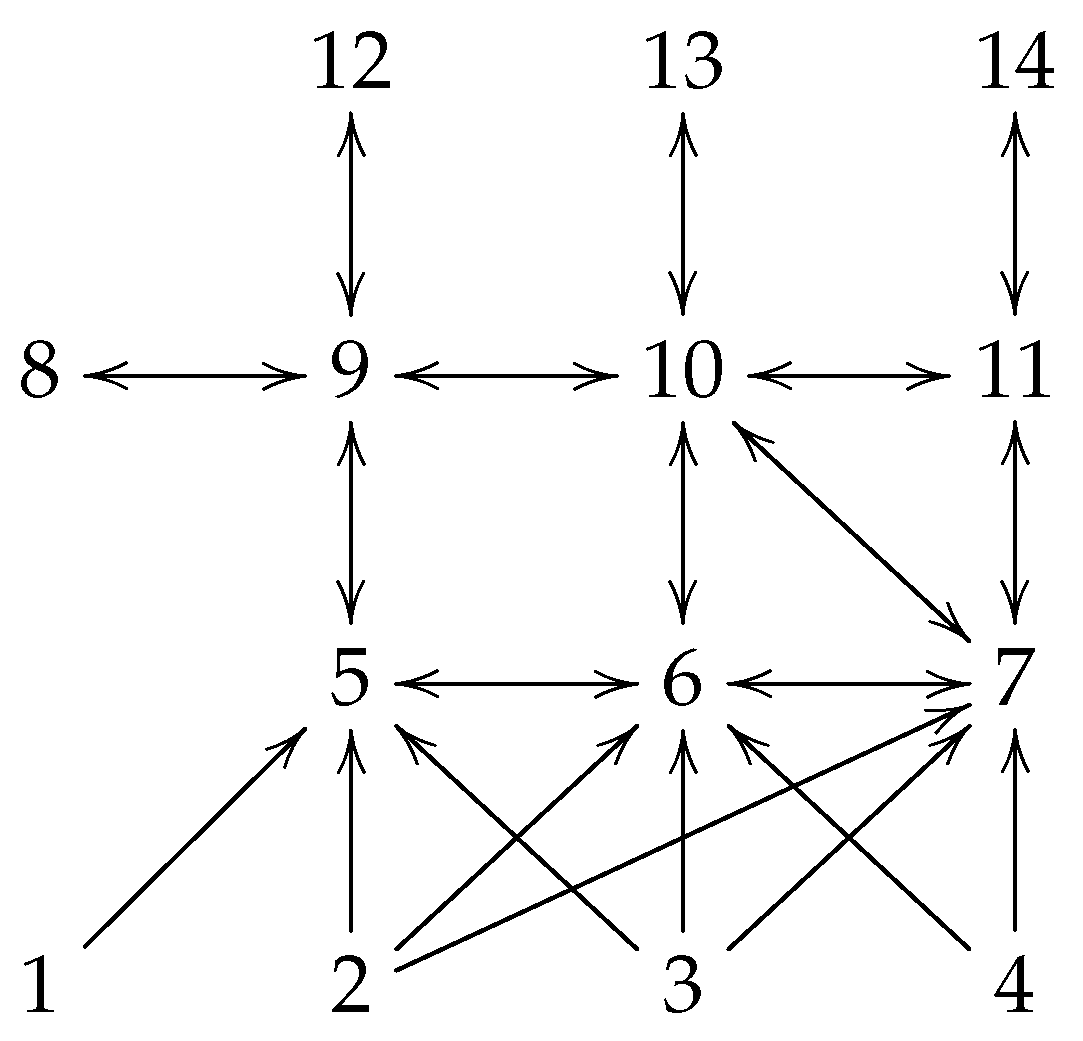
The network graph associated with the 14 agents is shown by Figure 1, and the corresponding Laplacian matrices are as following

$$\begin{array}{c}\hfill L_1=\left[\begin{array}{cccc}-1& -1& -1& 0\\ 0& -1& -1& -1\\ 0& -1& -1& -1\\ 0& 0& 0& 0\\ 0& 0& 0& 0\\ 0& 0& 0& 0\\ 0& 0& 0& 0\\ 0& 0& 0& 0\\ 0& 0& 0& 0\\ 0& 0& 0& 0\end{array}\right],L_2=\left[\begin{array}{cccccccccc}5& -1& 0& 0& -1& 0& 0& 0& 0& 0\\ -1& 6& -1& 0& 0& -1& 0& 0& 0& 0\\ 0& -1& 6& 0& 0& -1& -1& 0& 0& 0\\ 0& 0& 0& -1& -1& 0& 0& 0& 0& 0\\ -1& 0& 0& -1& 4& -1& 0& -1& 0& 0\\ 0& -1& -1& 0& -1& 5& -1& 0& -1& 0\\ 0& 0& -1& 0& 0& -1& 3& 0& 0& -1\\ 0& 0& 0& 0& -1& 0& 0& -1& 0& 0\\ 0& 0& 0& 0& 0& -1& 0& 0& -1& 0\\ 0& 0& 0& 0& 0& 0& -1& 0& 0& -1\end{array}\right].\end{array}$$

It is easy to obtain that the smallest eigenvalue of $L_2$ is ${\lambda }_1=0.2845$.

Containment control without input delay. We verify the effectiveness of containment control algorithm (20) and trigger function (18) first. Chose $a=1$. By solving matrix equality (25) we can obtain $P=\left[\begin{array}{cccc}1.5839& 0& 0.7543& 0\\ 0& 1.5839& 0& 0.7543\\ 0.7543& 0& 1.1947& 0\\ 0& 0.7543& 0& 1.1947\end{array}\right]$. According to Theorem 1, we can set K as

$$\begin{array}{c}\hfill K=-B^{T}P=\left[\begin{array}{cccc}0.7543& 0& 1.1947& 0\\ 0& 0.7543& 0& 1.1947\end{array}\right].\end{array}$$

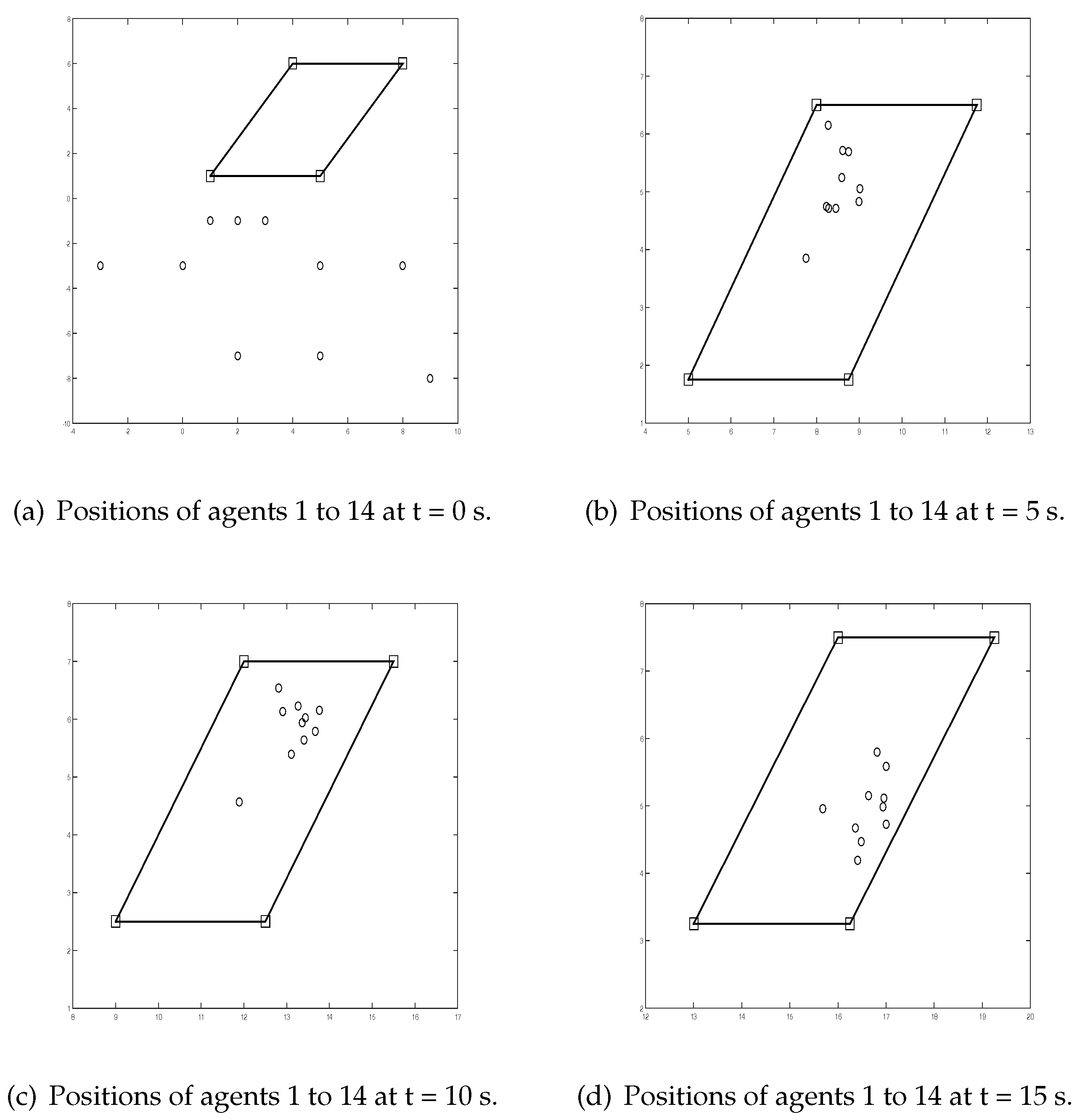
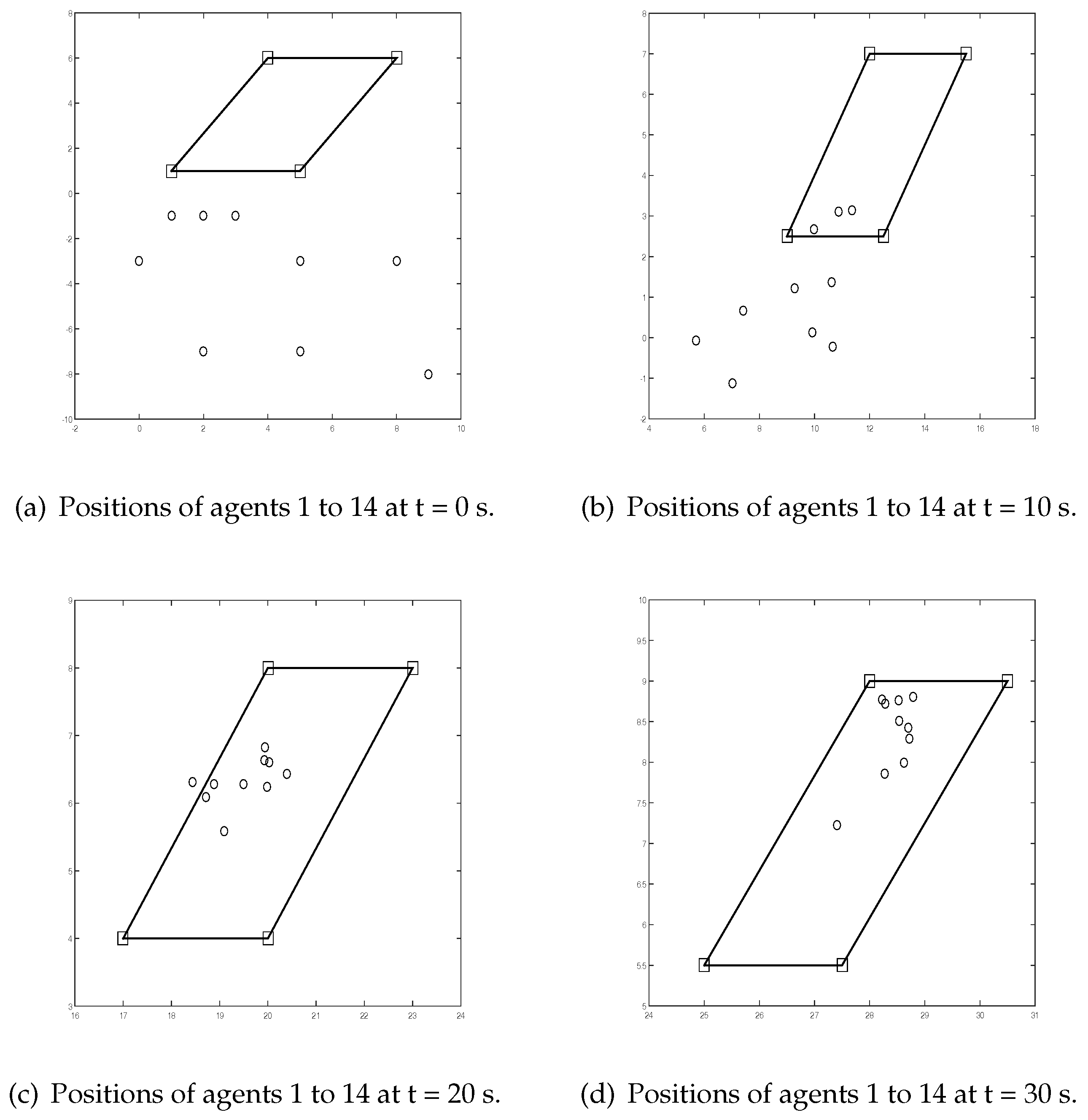
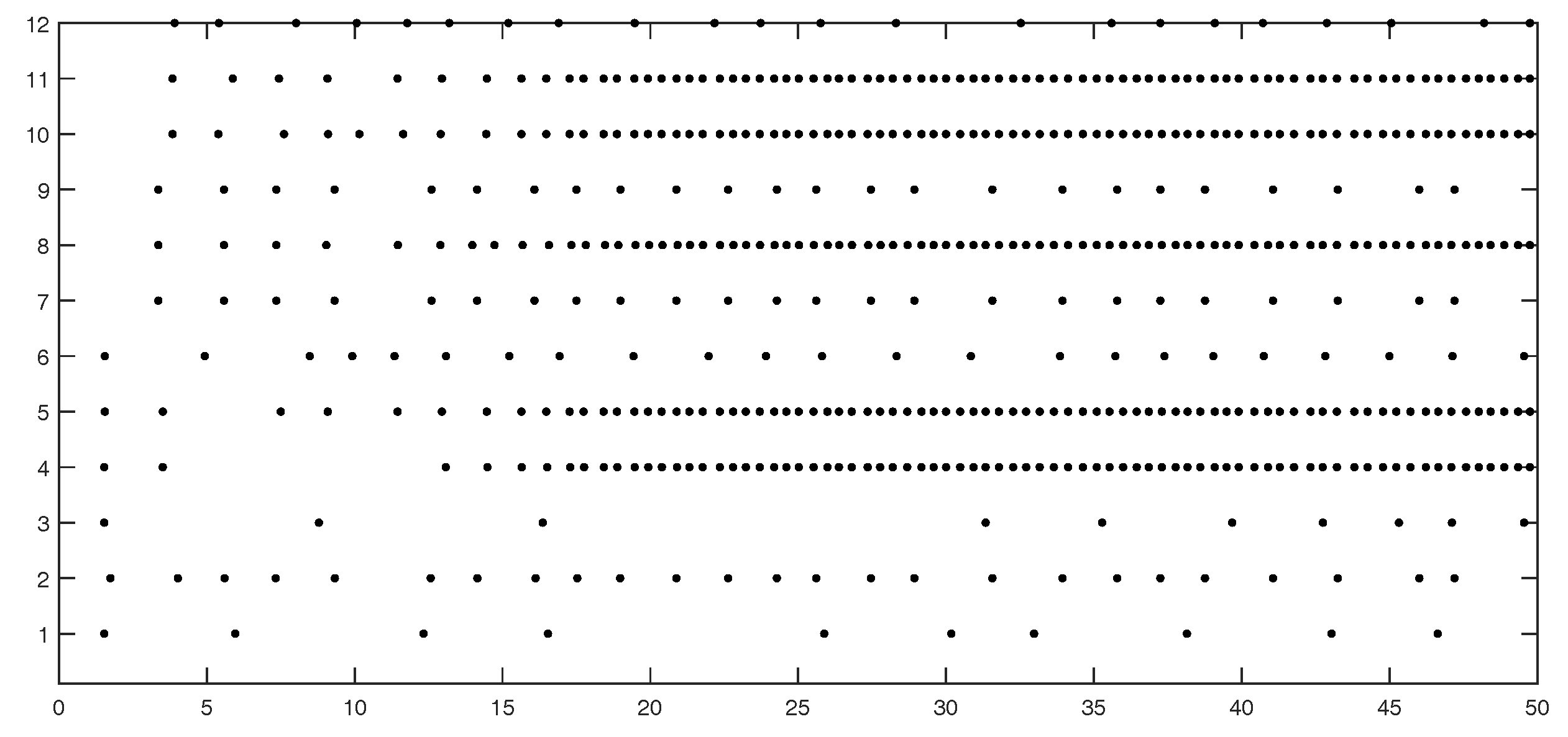
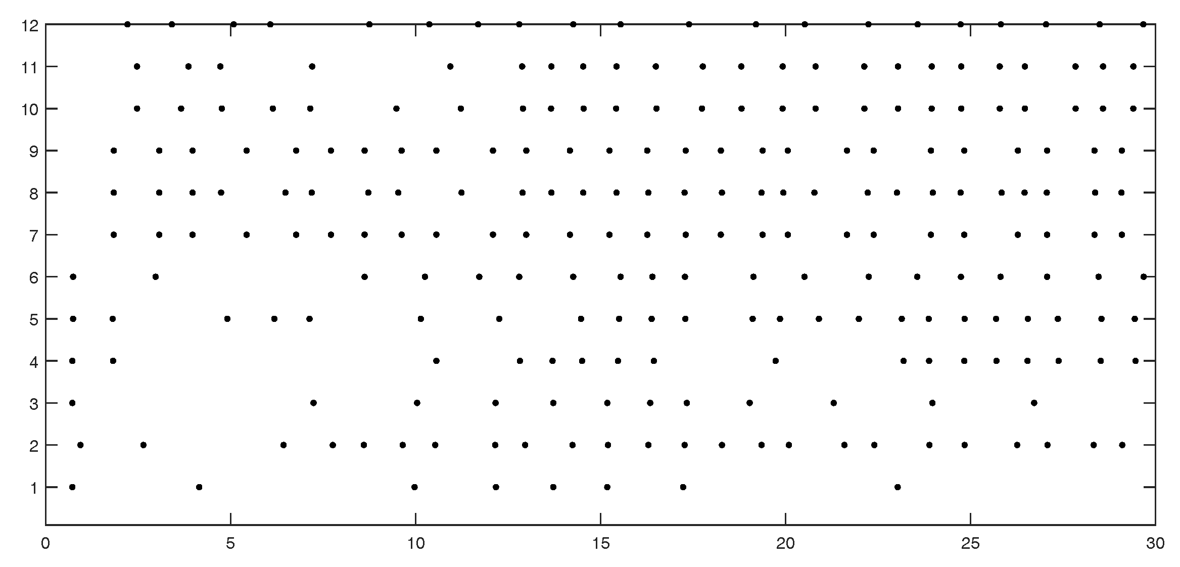
Let $\alpha =1$, $c=0.01$. Figure 2 shows positions of vehicles 1 to 14 at time instants 0 s, 5 s, 10 s, and 15 s. It can be seen that agents 5 to 14 move into the convex hull spanned by agents 1 to 4. Figure 3 shows the event instants on edges 1 to 12.

Table 1. Number of event instants of each edge ($\tau =0$, 15 s).

edge	1	2	3	4	5	6	7	8	9	10	11	12
connected agents	5–6	5–9	6–7	6–10	7–10	7–11	8–9	9–10	9–12	10–11	10–13	11–14
number of event instants	9	19	8	40	40	16	26	31	25	39	38	23

and

Table 2. Number of event instants of each agent ($\tau =0$, 15 s).

agent	5	6	7	8	9	10	11	12	13	14
number of event instants	28	57	64	26	101	198	78	25	38	23

show numbers of event instants counted by edge and agent, respectively. From Table 2 we can see that for most agents, the communication burden is light. However, for agents with many neighbor edges (agents 9–11), their communication burdens are heavy.

Containment control with input delay. Let $\tau =0.1$ s. By solving parametric Riccati Equation (5) with $\gamma =0.001$, we can obtain $P=\left[\begin{array}{cccc}0.0080& 0& 0.0316& 0\\ 0& 0.0080& 0& 0.0316\\ 0.0316& 0& 0.2535& 0\\ 0& 0.0316& 0& 0.2535\end{array}\right]$. Let $\mu =2$. According to Theorem 3, we can set K as

$$\begin{array}{c}\hfill K=-\mu B^{T}P=\left[\begin{array}{cccc}0.0632& 0& 0.5069& 0\\ 0& 0.0632& 0& 0.5069\end{array}\right].\end{array}$$

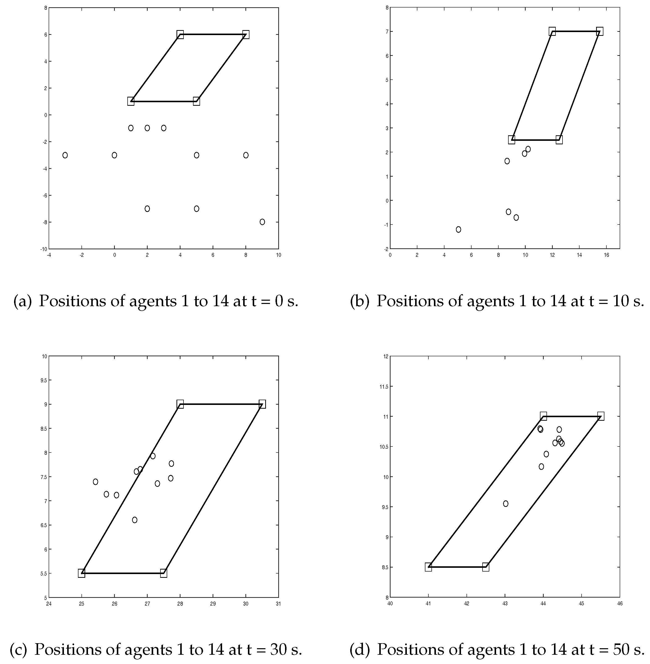
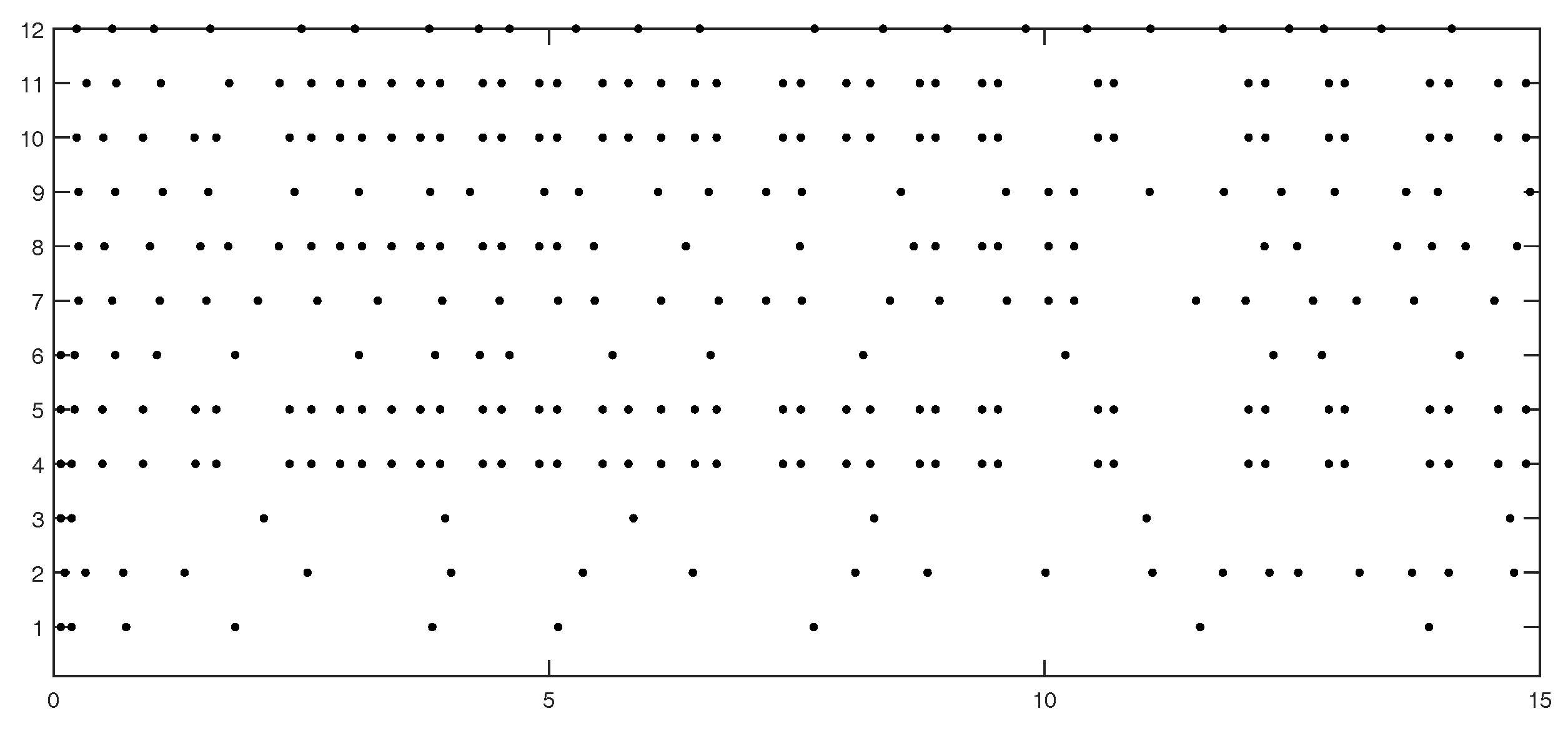
Figure 4 shows positions of agents 1 to 14 using Algorithm 2. It can be seen that agents 5 to 14 move into the convex hull spanned by vehicles 1 to 4. Figure 5 shows the event instants on edges 1 to 12.

Table 3. Number of event instants of each edge ($\tau =0.1$, 30 s).

edge	1	2	3	4	5	6	7	8	9	10	11	12
connected agents	5–6	5–9	6–7	6–10	7–10	7–11	8–9	9–10	9–12	10–11	10–13	11–14
number of event instants	8	24	12	17	23	19	26	28	26	25	23	20

and

Table 4. Number of event instants of each agent ($\tau =0.1$, 30 s).

agent	5	6	7	8	9	10	11	12	13	14
number of event instants	32	37	54	26	114	116	44	26	23	20

show numbers of event instants counted by edge and by agent, respectively.

Suppose that $\tau =0.5$ s. By solving parametric Riccati Equation (5) with $\gamma =0.0002$, we can obtain $P=\left[\begin{array}{cccc}0.0024& 0& 0.0141& 0\\ 0& 0.0024& 0& 0.0141\\ 0.0141& 0& 0.1688& 0\\ 0& 0.0141& 0& 0.1688\end{array}\right]$. Let $\mu =2$. According to Theorem 3, we can set K as

$$\begin{array}{c}\hfill K=-\mu B^{T}P=\left[\begin{array}{cccc}0.0283& 0& 0.3375& 0\\ 0& 0.0283& 0& 0.3375\end{array}\right].\end{array}$$

Figure 6 shows positions of agents 1 to 14. It can be seen that agents 5 to 14 move into the convex hull spanned by vehicles 1 to 4. Figure 7 shows the event instants on edges 1 to 12.

Table 5. Number of event instants of each edge ($\tau =0.1$, 50 s).

edge	1	2	3	4	5	6	7	8	9	10	11	12
connected agents	5–6	5–9	6–7	6–10	7–10	7–11	8–9	9–10	9–12	10–11	10–13	11–14
number of event instants	10	25	10	77	80	23	24	81	24	81	80	22

and

Table 6. Number of event instants of each agent ($\tau =0.5$, 50 s).

agent	5	6	7	8	9	10	11	12	13	14
number of event instants	35	97	113	24	154	399	104	24	80	22

show numbers of event instants counted by edge and by agent, respectively.

Remark 5.

From Figure 4 and Figure 6 we can see that the converge speed is lower when τ is larger. In fact, when the input delay τ is getting larger, according to Theorem 3, we should choose a smaller γ. From Lemma 3 we know that ${lim}_{\gamma \to 0^{+}}P(\gamma )=0$. So, when γ is small, the gain matrix K is small, which leads to low converge speed.

6. Conclusions

The event-triggered containment control problem has been considered in this paper, and two control algorithms have been proposed for multi-agent systems without and with input delay, respectively. Continuous communication has been avoided in the proposed triggering conditions. With the proposed algorithms, we have proved that all the followers can be driven into the convex hull formed by the leaders. When there is not input delay, it has been proved that the Zeno behavior can be avoided. Compared with some existing algorithms for the containment control problem with input delay, the proposed algorithm can deal with arbitrarily large input delay. The proposed triggering conditions can be detected dependently by each agent, while existing triggering conditions in those literatures on event-triggered containment control need to be realized in a centralized way.

References

1. Olfati-Saber, R.; Fax, J.A.; Murray, R.M. Consensus and cooperation in networked multi-agent systems. Proc. IEEE 2007, 95, 215–233. [Google Scholar] [CrossRef]
2. Ren, W.; Beard, R.W. Distributed Consensus in Multi-Vehicle Cooperative Control; Springer: London, UK, 2008; ISBN 978-1-84800-014-8. [Google Scholar]
3. Cao, M.; Morse, A.S.; Anderson, B.D.O. Agreeing asynchronously. IEEE Trans. Autom. Control 2008, 53, 1826–1838. [Google Scholar] [CrossRef]
4. Cao, Y.; Yu, W.; Ren, W.; Chen, G. An overview of recent progress in the study of distributed multi-agent coordination. IEEE Trans. Ind. Inform. 2013, 9, 427–438. [Google Scholar] [CrossRef]
5. Gulzar, M.M.; Rizvi, S.T.H.; Javed, M.Y.; Munir, U.; Asif, H. Multi-agent cooperative control consensus: A comparative review. Electronics 2018, 7, 22. [Google Scholar] [CrossRef]
6. Ji, M.; Ferrari-Trecate, G.; Egerstedt, M.; Buffa, A. Containment control in mobile networks. IEEE Trans. Autom. Control 2008, 53, 1972–1975. [Google Scholar] [CrossRef]
7. Cao, Y.; Stuart, D.; Ren, W.; Meng, Z. Distributed containment control for multiple autonomous vehicles with double-integrator dynamics: algorithms and experiments. IEEE Trans. Control Syst. Technol. 2011, 19, 929–938. [Google Scholar] [CrossRef]
8. Cao, Y.; Ren, W.; Egerstedt, M. Distributed containment control with multiple stationary or dynamic leaders in fixed and switching directed networks. Automatica 2012, 48, 1586–1597. [Google Scholar] [CrossRef]
9. Shi, G.; Hong, Y.; Johansson, K.H. Connectivity and set tracking of multi-agent systems guided by multiple moving leaders. IEEE Trans. Autom. Control 2012, 57, 663–676. [Google Scholar] [CrossRef]
10. Lou, Y.; Hong, Y. Target containment control of multi-agent systems with random switching interconnection topologies. Automatica 2012, 48, 879–885. [Google Scholar] [CrossRef]
11. Meng, Z.; Ren, W.; You, Z. Distributed finite-time attitude containment control for multiple rigid bodies. Automatica 2010, 46, 2092–2099. [Google Scholar] [CrossRef]
12. Qin, J.; Zheng, W.; Gao, H.; Ma, Q.; Fu, W. Containment control for second-order multiagent systems communicating over heterogeneous networks. IEEE Trans. Neural Netw. Learn. Syst. 2017, 28, 2143–2155. [Google Scholar] [CrossRef] [PubMed]
13. Li, J.; Ren, W.; Xu, S. Distributed containment control with multiple dynamic leaders for double-integrator dynamics using only position measurements. IEEE Trans. Autom. Control 2012, 57, 1553–1559. [Google Scholar] [CrossRef]
14. Liu, H.; Xie, G.; Wang, L. Containment of linear multi-agent systems under general interaction topologies. Syst. Control Lett. 2012, 61, 528–534. [Google Scholar] [CrossRef]
15. Li, Z.; Ren, W.; Liu, X.; Fu, M. Distributed containment control of multi-agent systems with general linear dynamics in the presence of multiple leaders. Int. J. Robust Nonlinear Control 2013, 23, 534–547. [Google Scholar] [CrossRef]
16. Wen, G.; Zhao, Y.; Duan, Z.; Yu, W.; Chen, G. Containment of higher-order multi-leader multi-agent systems: A dynamic output approach. IEEE Trans. Autom. Control 2015, 61, 1135–1140. [Google Scholar] [CrossRef]
17. Cheng, L.; Wang, Y.; Ren, W.; Hou, Z.-G.; Tan, M. Containment control of multiagent systems with dynamic leaders based on a PIn-Type approach. IEEE Trans. Cybern. 2016, 46, 3004–3017. [Google Scholar] [CrossRef] [PubMed]
18. Tabuada, P. Event-triggered real-time scheduling of stabilizing control tasks. IEEE Trans. Autom. Control 2007, 52, 1680–1685. [Google Scholar] [CrossRef]
19. Zhang, B.-L.; Han, Q.-L.; Zhang, X.-M. Event-triggered H control for offshore structures in network environments. J. Sound Vib. 2016, 368, 1–21. [Google Scholar] [CrossRef]
20. Zhang, X.-M.; Zhang, Q.-L. A decentralized event-triggered dissipative control scheme for systems with multiple sensors to sample the system outputs. IEEE Trans. Cybern. 2016, 46, 2745–2757. [Google Scholar] [CrossRef] [PubMed]
21. Wang, Y.-L.; Shi, P.; Lim, C.-C.; Liu, Y. Event-triggered fault detection filter design for a continuous-time networked control system. IEEE Trans. Cybern. 2016, 46, 3414–3426. [Google Scholar] [CrossRef] [PubMed]
22. Wang, Y.-L.; Shi, P.; Lim, C.-C. Adaptively adjusted event-triggering mechanism on fault detection for networked control systems. IEEE Trans. Cybern. 2017, 47, 2299–2311. [Google Scholar] [CrossRef] [PubMed]
23. Zhang, X.-M.; Han, Q.-L. Network-based H filtering using a logic jumping-like trigger. Automatica 2013, 49, 1428–1435. [Google Scholar] [CrossRef]
24. Yue, D.; Tian, E.; Han, Q.-L. A delay system method for designing event-triggered controllers of networked control systems. IEEE Trans. Autom. Control 2013, 58, 475–481. [Google Scholar] [CrossRef]
25. Zhang, X.-M.; Han, Q.-L.; Zhang, B.-L. An overview and deep investigation on sampled-data-based event-triggered control and filtering for networked systems. IEEE Trans. Ind. Inform. 2016, 13, 4–16. [Google Scholar] [CrossRef]
26. Li, Y.; Liu, X.; Peng, L. An event-triggered fault detection approach in cyber-physical systems with sensor nonlinearities and deception attacks. Electronics 2018, 7, 168. [Google Scholar] [CrossRef]
27. Dimarogonas, D.V.; Frazzoli, E.; Johansson, K.H. Distributed event-triggered control for multi-agent systems. IEEE Trans. Autom. Control 2012, 57, 1291–1297. [Google Scholar] [CrossRef]
28. Seyboth, G.S.; Dimarogonas, D.V.; Johansson, K.H. Event-based broadcasting for multi-agent average consensus. Automatica 2013, 49, 245–252. [Google Scholar] [CrossRef]
29. Wu, Y.; Meng, X.; Xie, L.; Lu, R.; Su, H. An input-based trigging approach to leader-following problems. Automatica 2017, 5, 221–228. [Google Scholar] [CrossRef]
30. Ding, L.; Han, Q.-L.; Ge, X.; Zhang, X.M. An overview of recent advances in event-triggered consensus of multiagent systems. IEEE Trans. Cybern. 2018, 48, 1110–1123. [Google Scholar] [CrossRef] [PubMed]
31. Xia, H.; Zheng, W.; Shao, J. Event-triggered containment control for second-order multi-agent systems with sampled position data. ISA Trans. 2018, 73, 91–99. [Google Scholar] [CrossRef] [PubMed]
32. Zou, W.; Xiang, Z. Event-triggered distributed containment control of heterogeneous linear multi-agent systems by an output regulation approach. Int. J. Syst. Sci. 2017, 48, 2041–2054. [Google Scholar] [CrossRef]
33. Zou, W.; Xiang, Z. Event-triggered containment control of second-order nonlinear multi-agent systems. J. Frankl. Inst. 2018. [Google Scholar] [CrossRef]
34. Zhang, B.-L.; Han, Q.-L.; Zhang, X.-M.; Yu, X. Sliding mode control with mixed current and delayed states for offshore steel jacket platform. IEEE Trans. Control Syst. Technol. 2014, 22, 1769–1783. [Google Scholar] [CrossRef]
35. Xiao, S.-P.; Xu, L.; Zeng, H.; Teo, K. Improved stability criteria for discrete-time delay systems via novel summation inequalities. Int. J. Control Autom. Syst. 2018, 16, 1592–1602. [Google Scholar] [CrossRef]
36. Xiao, S.-P.; Lian, H.; Teo, K.; Zeng, H.-B.; Zhang, X.-H. A new Lyapunov functional approach to sampled-data synchronization control for delayed neural networks. J. Frankl. Inst. 2018, 355, 8857–8873. [Google Scholar] [CrossRef]
37. Zhang, X.-M.; Han, Q.-L. Abel lemma-based finite-sum inequality and its application to stability analysis for linear discrete time-delay system. Automatica 2015, 57, 199–202. [Google Scholar] [CrossRef]
38. Xu, S.; Lam, J. On equivalence and efficiency of certain stability criteria for time-delay systems. IEEE Trans. Autom. Control 2007, 52, 95–101. [Google Scholar] [CrossRef]
39. Zhang, B.; Zheng, W.; Xu, S. Filtering of markovian jump delay systems based on a new performance index. IEEE Trans. Circuits Syst.-I Regul. Pap. 2013, 60, 1250–1263. [Google Scholar] [CrossRef]
40. Ma, Q.; Feng, G.; Xu, S. Delay-dependent stability criteria for reaction–diffusion neural networks with time-varying delays. IEEE Trans. Cybern. 2013, 43, 1913–1920. [Google Scholar] [CrossRef] [PubMed]
41. Zhou, B.; Lin, Z. Consensus of high-order multi-agent systems with large input and communication delays. Automatica 2014, 50, 452–464. [Google Scholar] [CrossRef]
42. Liu, K.; Xie, G.M.; Wang, L. Containment control for second-order multi-agent systems with time-varying delays. Syst. Cont. Lett. 2014, 67, 24–31. [Google Scholar] [CrossRef]
43. Miao, G.; Cao, J.; Alsaedi, A.; Alsaadi, F.E. Event-triggered containment control for multi-agent systems with constant time delays. J. Frankl. Inst. 2017, 354, 6956–6977. [Google Scholar] [CrossRef]
Figure 1. The network topology associated with vehicles 1 to 14. Here i denotes vehicle i, i = 1 , , 14 .
Electronics 07 00343 g001
Figure 2. Positions of agents 1 to 14 using Algorithm 1, where squares denote leaders and circles denote followers.
Electronics 07 00343 g002
Figure 3. Event instants on edges 1–12 ( τ = 0 , 15 s).
Electronics 07 00343 g003
Figure 4. Positions of agents 1 to 14 using Algorithm 2 with τ = 0.1 , where squares denote leaders and circles denote followers.
Electronics 07 00343 g004
Figure 5. Event instants on edges 1–12 ( τ = 0.1 , 30 s).
Electronics 07 00343 g005
Figure 6. Positions of agents 1 to 14 using Algorithm 2 with τ = 0.5 , where squares denote leaders and circles denote followers.
Electronics 07 00343 g006
Figure 7. Event instants on edges 1–12 ( τ = 0.5 , 50 s).
Electronics 07 00343 g007