Article

A Nonlinearly Modulated Logistic Map with Delay for Image Encryption

School of Information Science and Engineering, Lanzhou University, Lanzhou 730000, China
*
Author to whom correspondence should be addressed.
Electronics 2018, 7(11), 326; https://doi.org/10.3390/electronics7110326
Submission received: 10 October 2018 / Revised: 8 November 2018 / Accepted: 12 November 2018 / Published: 15 November 2018
(This article belongs to the Special Issue Recent Developments on Time-Delay Systems and Its Applications)

Abstract

:
Considering that a majority of the traditional one-dimensional discrete chaotic maps have disadvantages including a relatively narrow chaotic range, smaller Lyapunov exponents, and excessive periodic windows, a new nonlinearly modulated Logistic map with delay model (NMLD) is proposed. Accordingly, a chaotic map called a first-order Feigenbaum-Logistic NMLD (FL-NMLD) is proposed. Simulation results demonstrate that FL-NMLD has a considerably wider chaotic range, larger Lyapunov exponents, and superior ergodicity compared with existing chaotic maps. Based on FL-NMLD, we propose a new image encryption algorithm that joins the pixel plane and bit-plane shuffle (JPB). The simulation and test results confirm that JPB has higher security than simple pixel-plane encryption and is faster than simple bit-plane encryption. Moreover, it can resist the majority of attacks including statistical and differential attacks.

1. Introduction

Because of pseudo-randomness, orbital unpredictability, and sensitivity of the initial values, chaotic maps have been widely applied in the encryption system, especially image encryption [1,2,3,4,5,6,7,8,9,10]. For example, a symmetric image encryption algorithm based on mixed linear-nonlinear coupled map lattice was proposed by Zhang et al. [11], a novel image encryption algorithm based on cycle shift and chaotic system was proposed by Wang et al. [4], and an image encryption algorithm using the two-dimensional logistic chaotic map was proposed by Wu et al. [1].
One-dimensional (1D) chaotic maps, such as Logistic map [12], usually have relatively narrow chaotic range, smaller Lyapunov exponent, and excessive periodic windows, and their structure and chaotic orbit are rather simple. With the development of chaotic cracking technology, the trajectory of 1D chaotic maps may be estimated [13]. So using 1D chaotic maps in image encryption may be insecure. There is a report that Logistic map-based image encryption algorithm proposed in [14] was proved to be not safe [15].
To address the disadvantages of 1D chaotic maps, researchers have developed several methods. In [16], a two-dimensional (2D) Sine Logistic modulation map (2D-SLMM) is proposed combining a 1D Logistic map and sinusoidal map. In [17], a new 1D chaotic map is constructed by superimposing any two chaotic maps from Logistic, sinusoidal, and tent maps. In [18], Zhou et al. designed a new parameter switching chaotic system and applied this to image encryption.
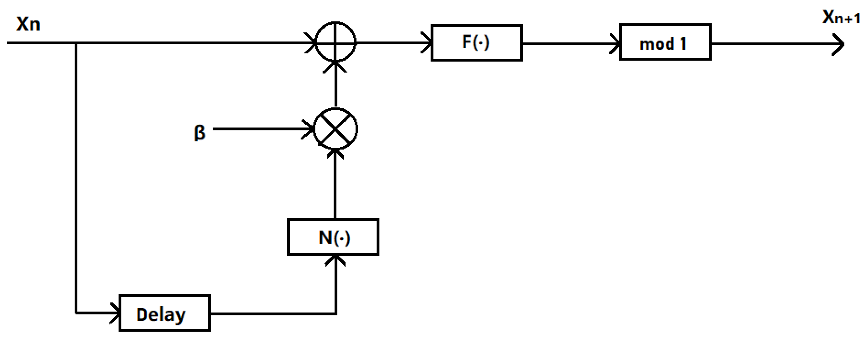
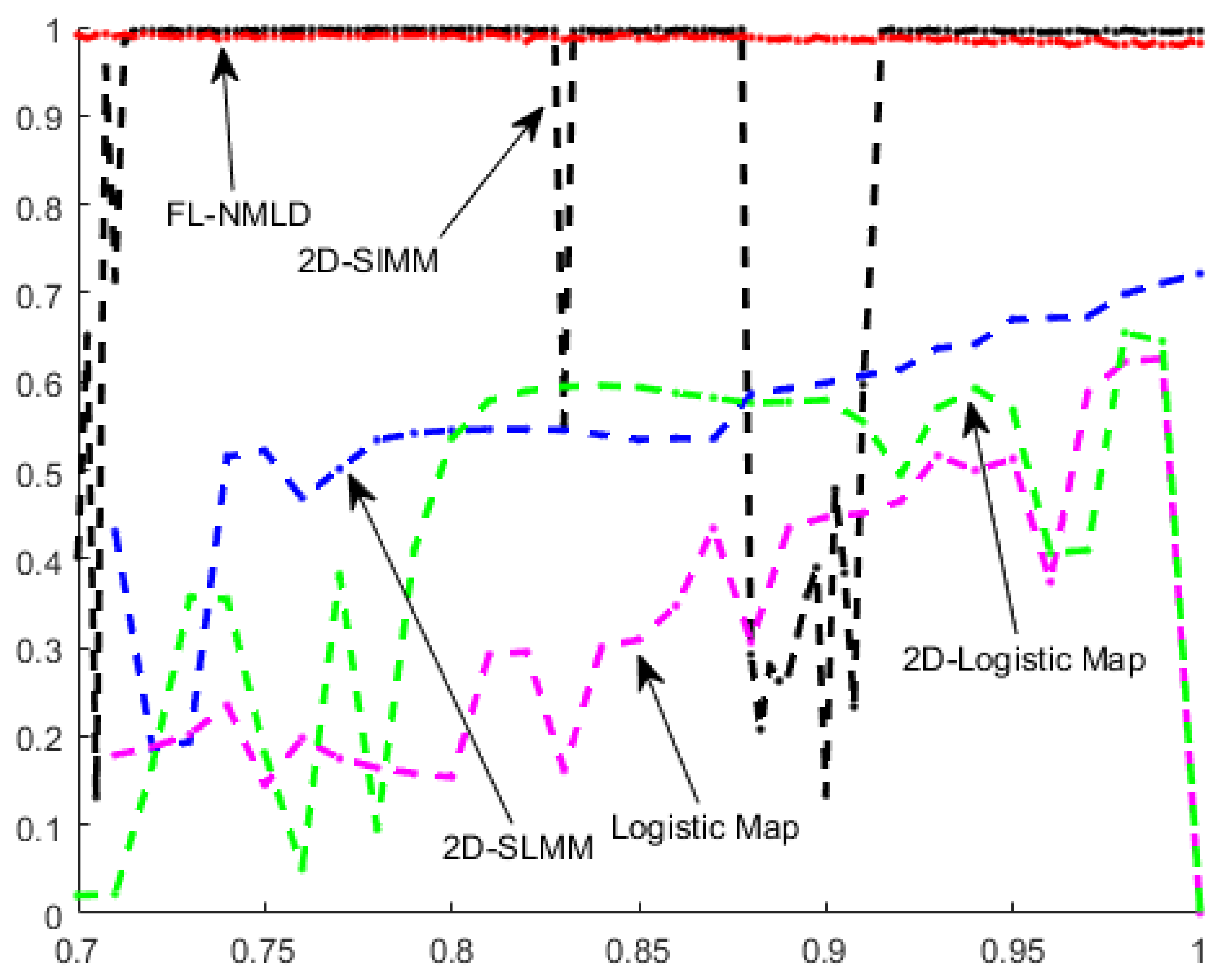
However, the chaotic maps proposed in these papers realise better performance only by increasing the nonlinearity of the chaotic map. In this study, we add delay and nonlinear modulation into the 1D chaotic map [19] and propose a new nonlinearly modulated Logistic map with delay model (NMLD). Since the parameter of Logistic map varies over a larger range than most other chaotic maps, such as Bernoulli map, applying it to our model may result in a larger chaotic interval, which provides greater key space when encrypting. So, we propose a chaotic map called first-order Feigenbaum-Logistic NMLD (FL-NMLD) based on our model. It has a considerably wider chaotic range, larger Lyapunov exponents, and superior ergodicity compared to existing chaotic maps.
The shuffle process can operate on the pixel-plane or bit-plane. A majority of recent image encryption algorithms operate on the pixel plane [4,16,20,21]. The pixel-plane shuffle operation of these algorithms just changes the position of the pixel. Conversely, bit-plane shuffle not only changes the position of the pixel, but also changes the position of each bit in the pixel, so it is more secure; however, it requires more execution time. In this paper, we propose a image encryption algorithm that joins pixel-plane and bit-plane shuffle (JPB). This algorithm performs different encryption operations on one or several bit planes according to the amount of information contained in each bit plane. Compared to simple pixel-plane encryption [4] and simple bit-plane encryption [22], this image encryption algorithm balances the security of the encryption system with time consumption.
The remainder of this paper is organised as follows. In Section 2, the NMLD model is proposed and its chaotic characteristics are analysed using trajectory, Lyapunov exponents, and permutation entropy. In Section 3, the JPB image encryption algorithm based on FL-NMLD is presented. In Section 4, we analyse the security and time complexity of JPB. Finally, we summarise the results.

2. Nonlinearly Modulated Logistic Map with Delay

2.1. NMLD Model

The new nonlinearly modulated Logistic map with delay model (NMLD) is displayed in Figure 1. The role of the + block is to add the input, and the role of the X block is to multiply the input. The mathematical formula for this model is Equation (1).
x n + 1 = m o d ( F ( x n + β N ( x n 1 ) ) , 1 )
where F ( · ) is a 1D chaotic map, N ( · ) is a nonlinear item, and m o d ( x , 1 ) is the remainder of x divided by one. The parameter β [0, 1] and x n 1 is the delay item of x n . We can add more delay items to this model and change the selection of F ( · ) and N ( · ) . Hence, this model is extensible.

2.2. First-Order Delay Feigenbaum-Logistic NMLD

In the NMLD model, when F ( x ) is set as a traditional 1D Logistic map and N ( x ) is set as the Feigenbaum formula [23], we can obtain the FL-NMLD as Equation (2) indicates.
x n + 1 = m o d ( F ( x n + β s i n ( π x n 1 ) ) , 1 ) = m o d ( α ( x n + β s i n ( π x n 1 ) ) ( 1 ( x n + β s i n ( π x n 1 ) ) ) , 1 )
where α and β are parameters, α [ 0 , 4 ] , β [0, 1]. x n 1 is the delay item of x n . As β increases, the properties of the chaotic system improve. For simplicity, β is set to 1 in the remainder of this paper.

2.3. Performance Evaluation of FL-NMLD

To evaluate the performance of FL-NMLD, we analyse this chaotic map using trajectory, Lyapunov exponent [24], and permutation entropy [25].

2.3.1. Trajectory

Figure 2 displays the trajectories of FL-NMLD, 2D-SLMM [16], and 2D-SIMM [21]. The larger the region where the trajectory distributes, the better the ergodicity of the chaotic map. From the figure, we can observe that the trajectory of FL-NMLD distributes in a larger region than 2D-SLMM and 2D-SIMM, virtually covering the entire phase plane. This means FL-NMLD has excellent ergodicity. Further, using this map, we can obtain sequences that have superior randomness.

2.3.2. Lyapunov Exponent

Initial sensitivity is an important property of a chaos system. This means the trajectories of two similar initial values that evolve through systematic evolution are exponentially separated over time, which causes the system’s future state to be unpredictable. The Lyapunov exponent can be used to quantitatively describe the initial sensitivity of a chaos system. For delay differential equations, the number of positive Lyapunov exponents increases linearly with the delay [26,27,28]. There is a delay item in the FL-NMLD equation; hence, FL-NMLD has two positive Lyapunov exponents.
We increase the parameter of chaotic map by 0.05 each time to draw a Lyapunov exponent, and the results are shown in Figure 3. From Figure 3b, we can observe that λ 1 is greater than zero when α [0.885, 1], which means 2D-SLMM is chaotic in this range. Further, if the number of directions of spreading is more than one, the system has hyperchaotic behavior [29]. Both λ 1 and λ 2 are greater than zero when α [0.905, 1], which means 2D-SLMM is hyperchaotic in this range.
As indicated in Figure 3c, 2D-SIMM is virtually chaotic when α [0.7, 4], except for three large periodic windows, and is hyperchaotic when α [0.7, 2.7]. The three large periodic windows make the available chaotic range discontinuous.
As indicated in Figure 3a, FL-NMLD is chaotic when α [1.1, 4] and is hyperchaotic when α [1.1, 2] and [2.1, 4]. The greatest advantage of FL-NMLD is that it has a considerably wider chaotic range and there is no periodic window. This means it has more available continuous chaotic range. Further, it is beneficial to have a larger key space when this map is used for image encryption. Moreover, the maximum Lyapunov exponent (MLE) of FL-NMLD is relatively large, which means it is difficult to predict the chaotic sequence.

2.3.3. Permutation Entropy

Permutation entropy (PE) is a useful method to indicate the complication of chaotic dynamical systems; the greater the entropy, the more complex the dynamical behaviours of the chaotic system. In the simulation, we calculate the PE using the method proposed in [25]. Figure 4 displays the PE of FL-NMLD, 2D-SLMM, 2D-SIMM, 2D-Logistic map, and Logistic map. Clearly, the PE value of FL-NMLD is greater than that of the other maps. The PE of 2D-SIMM is greater than FL-NMLD in certain ranges, although it has three large periodic windows. Conversely, the PE value of FL-NMLD is stable and is close to the ideal value of one. This means that FL-NMLD has more complex dynamical behaviours.

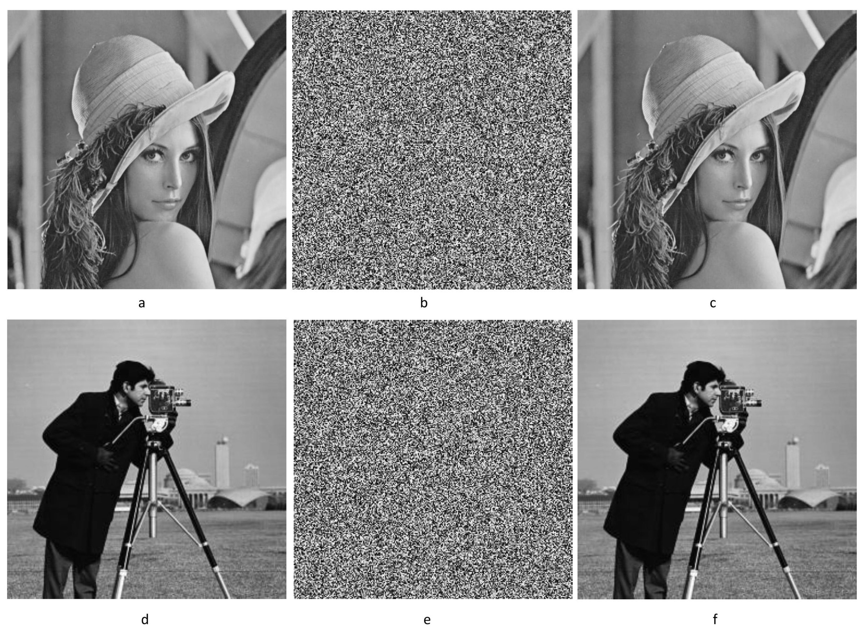
3. Joint Pixel-Plane and Bit-Plane Image Encryption

The shuffle process of an image encryption algorithm can operate on the pixel plane or bit plane. A pixel-plane shuffle has higher efficiency than bit-plane scrambling; however, its security is not sufficiently acceptable. Conversely, a bit-plane shuffle process is more secure; however, it requires more execution time.
The information contained in different bits may vary in one pixel. For example, a “1” at the 8th bit of a pixel represents 128 ( 2 7 ). In contrast, a “1” only represents 1 ( 2 0 ) at the first bit, which contains less information. According to Equation (3), we calculated the ratio p ( i ) of information contained in ith bit, as shown in Table 1.
p ( i ) = 2 i i = 0 7 2 i
Considering that more than 90% of the information of one pixel is concentrated in the higher four bits, we separate the higher four-bit planes to perform bit-plane shuffle. Simultaneously, we reassemble the lower four-bit planes into a pixel plane for pixel-plane shuffle. Then, through conversions, we can obtain eight shuffled bit planes. Next, after reassembling these bit planes into a pixel plane, we can obtain the shuffled image.
Then, we perform a diffusion operation to alter the value of each pixel in the shuffled image.
Based on the joint operations of bit and pixel plane, we propose an improved chaotic image encryption scheme, as displayed in Figure 5. In Figure 5, the symbol M N indicates the size of the matrix.
Moreover, the shuffle process is related to the plaintext; hence, the encrypted image can effectively resist chosen plaintext attacks.

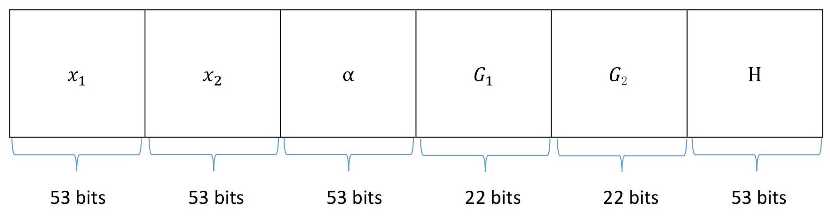
3.1. Secret Key Structure

Figure 6 displays the structure of the secret key. The key is 256 bits long. x 1 , x 2 , α , and H are decimals generated by a 53-bit string { b 53 , b 52 , , b 1 } according to the IEEE 754 format, as indicated in Equation (4).
x = i = 1 53 b i 2 i 1 2 53
The computational precision of the double-precision number is considered as 10 16 2 53 ; hence, x 1 , x 2 , α , and H are set as 53 bits long. G 1 and G 2 are integers generated by a 22-bit string. We can obtain the initial values x 1 , 1 , x 1 , 2 , x 2 , 1 , and x 2 , 2 , and chaotic parameters α 1 and α 2 of the chaotic map using Equation (5).
x 1 , i = m o d ( ( x 1 + G i H ) , 1 ) x 2 , i = m o d ( ( x 2 + G i H ) , 1 ) α i = 1.3 + m o d ( ( α + G i H ) , 0.1 )
where the value of i is ‘1’ or ‘2’.
To ensure that FL-NMLD has acceptable chaotic performance, the calculated initial values should be in the range of [0, 1], and the chaotic parameters should be limited to [1.1, 4].

3.2. Shuffle Process

Before performing the bit-plane and pixel-plane shuffle, the higher four-bit planes and lower four-bit planes must be first separated. Further, we must perform conversions to facilitate the shuffle process. Finally, we must obtain the chaotic sequence used for the shuffle based on the input secret key.
Input The security key K = { x 1 , x 2 , α , G 1 , G 2 , H} and plaintext image P with size of M N .
Step 1 Convert P into a binary matrix B, with size M N 8 . Each column of matrix B has the same elements as the bit plane.
Step 2 Separate the first four columns of B as B 1 , with size M N 4 . Reshape matrix B 1 into M 4 N to obtain matrix H B . Matrix H B is a combination of the higher four-bit planes. From the first five columns of H B in Figure 7, we can see how to get the H B matrix. The four elements of the first column in H B come from elements of the same color in B 1 , and the following columns are similar. We can use the reshape command in MATLAB to implement this transformation.
Step 3 Separate the last four columns of B as B 2 . Convert B 2 into a decimal matrix L B , with size M N 1 . Matrix L B is reassembled by the lower four-bit planes.
Figure 7 displays the process in Steps 1–3 using an example.
Step 4 Obtain the initial values x 1 , 1 and x 1 , 2 , and chaotic parameter α 1 based on secret key K, and update the initial value x 1 , 1 using Equation (6).
x ˙ 1 , 1 = m o d ( ( x 1 , 1 + s u m 1 ) , 1 )
where s u m 1 is calculated using Equation (7).
s u m 1 = i = 1 M N j = 1 8 B i , j M N
Step 5 Iterate Equation (2) ( M N + 4 N + M + r 1 ) times using the initial values x ˙ 1 , 1 and x 1 , 2 , and discard the former r 1 items to obtain sequence x. Then, let x 1 = x ( 1 : M N ) , x 2 = x ( M N + 1 : M N + M ) , and x 3 = x ( M N + M + 1 : M N + M + 4 N ) .

3.2.1. Bit-Plane Shuffle

In this process, we perform row and column cyclic shifts on H B , which is the combination of the higher four-bit planes.
Step 1 Rotate the ith row of matrix H B cyclically to the right r ( i ) times to obtain matrix H B 1 . r ( i ) is obtained by x 2 using Equation (8).
r ( i ) = f l o o r ( m o d ( x 2 ( i ) 10 6 , M ) )
where i = 1 , 2 , M and f l o o r ( x ) is the largest integer not greater than x.
Step 2 Cyclically shift the ith column of matrix H B 1 from top to bottom c ( i ) times to obtain matrix H B 2 . c ( i ) is obtained by x 3 using Equation (9).
c ( i ) = f l o o r ( m o d ( x 3 ( i ) 10 6 , 4 N ) )
where i = 1 , 2 , 4 N .

3.2.2. Pixel-Plane Shuffle

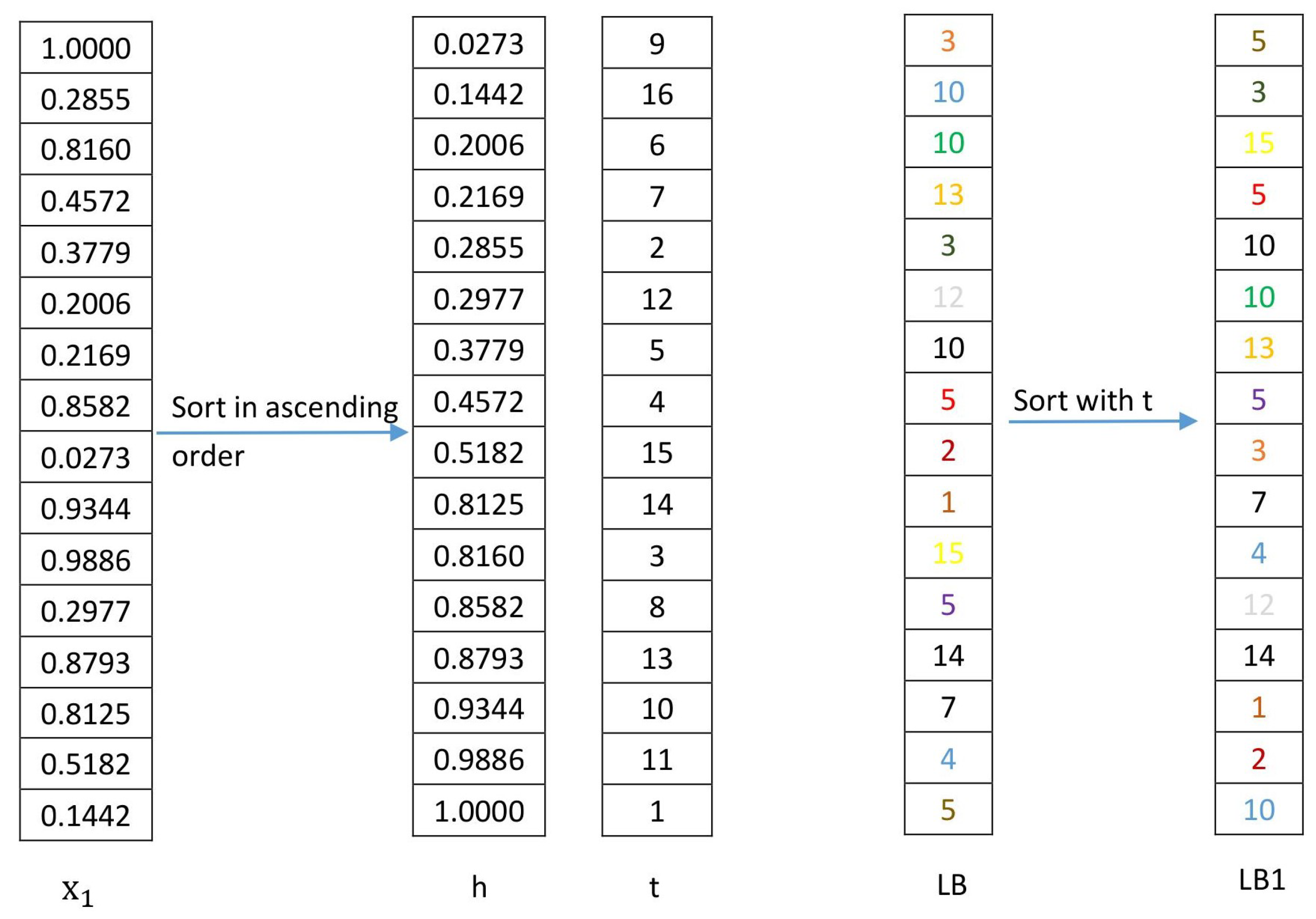
In this process, we use a chaotic sequence to sort matrix L B transformed from the lower four-bit planes.
Step 1 Sort the chaotic sequence x 1 in ascending order. Then, we can obtain the sorted sequence h and index sequence t.
Step 2 Sort matrix L B with t to obtain sorted matrix L B 1 . The specific method is illustrated below.
f o r i = 1 : M N
L B 1 ( t ( i ) ) = L B ( i )
Figure 8 displays the process of pixel-plane shuffle.
After the bit-plane and pixel-plane shuffle processes, we can obtain the shuffled matrices H B 2 and L B 1 . Then, according to the inverse process of the operations displayed in Figure 7, the two matrices are transformed to obtain the shuffled image Q.

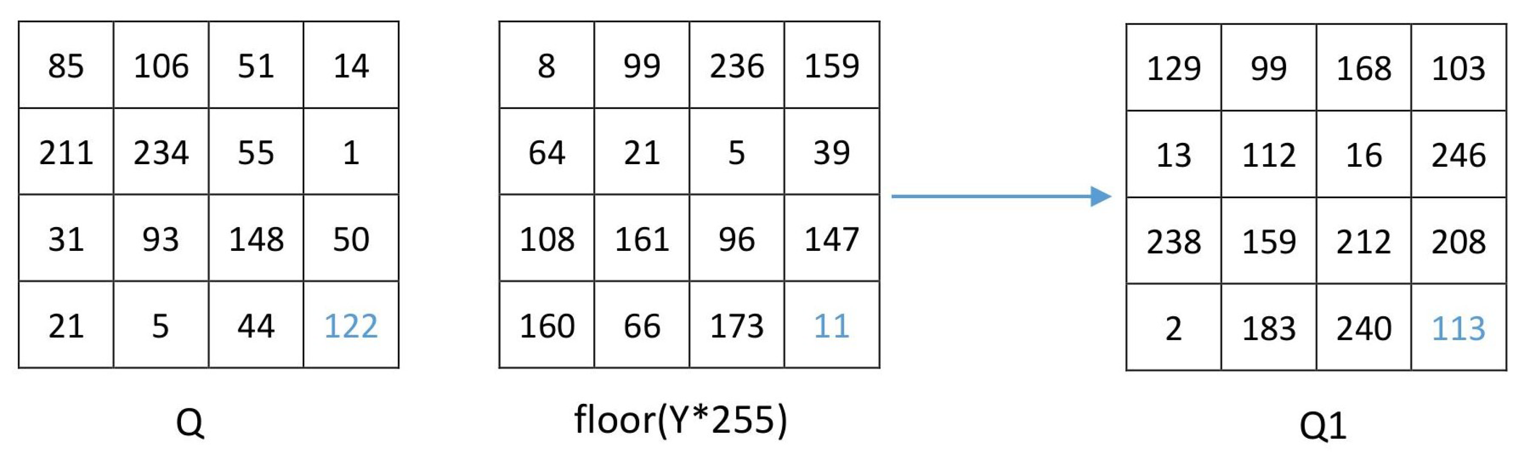
3.3. Diffusion Process

The diffusion process can alter the value of each pixel in the image to meet the requirement of the diffusion characteristic of the encryption algorithm. The diffusion strategy includes pixel-by-pixel diffusion [30] and block diffusion [31]. Pixel-by-pixel diffusion typically provides superior security compared to the others. Hence, in the proposed algorithm, we perform diffusion pixel-by-pixel.
Step 1 Obtain the initial values x 2 , 1 and x 2 , 2 , and chaotic parameter α 2 based on the secret key K.
Iterate Equation (2) ( M N + r 2 ) times with the initial values x 2 , 1 and x 2 , 2 , and discard the former r 2 items to obtain sequence y. Use the following formula to improve the randomness of the chaotic sequence.
y 1 = m o d ( y 10 7 , 1 ) ;
Then, reshape the sequence y 1 into matrix Y with size M N .
Step 2 Perform diffusion of the shuffled image Q; the specific method is displayed below.
f o r i = M : 1 : 1
f o r j = N : 1 : 1
i f i = = M & & j = = N
Q 1 ( i , j ) = Q ( i , j ) f l o o r ( Y ( i , j ) 255 )
e l s e i f i = = M & & 1 j < N
Q 1 ( i , j ) = Q ( i , j ) Q 1 ( i , j + 1 ) f l o o r ( Y ( i , j ) 255 )
e l s e i f 1 i < M & & j = = N
Q 1 ( i , j ) = Q ( i , j ) Q 1 ( i + 1 , j ) f l o o r ( Y ( i , j ) 255 )
e l s e i f 1 i < M & & 1 j < N
Q 1 ( i , j ) = Q ( i , j ) Q 1 ( i + 1 , j ) Q 1 ( i , j + 1 ) f l o o r ( Y ( i , j ) 255 )
where ⊕ is the operation where two numbers are bit-XORed by their binary values, and f l o o r ( x ) is the largest integer not greater than x. Q 1 is the encrypted image after diffusion.
An example of this process is provided below.
The diffusion process starts with i = M and j = N , which are the blue numbers in Figure 9. The specific calculation process is as follows:
Q 1 ( 4 , 4 ) = Q ( 4 , 4 ) f l o o r ( Y ( 4 , 4 ) 255 ) = 122 11 = 113
Q 1 ( 4 , 3 ) = Q ( 4 , 3 ) Q 1 ( 4 , 4 ) f l o o r ( Y ( 4 , 3 ) 255 ) = 44 113 173 = 240
Q 1 ( 4 , 2 ) = Q ( 4 , 2 ) Q 1 ( 4 , 3 ) f l o o r ( Y ( 4 , 2 ) 255 ) = 5 240 66 = 183
Q 1 ( 4 , 1 ) = Q ( 4 , 1 ) Q 1 ( 4 , 2 ) f l o o r ( Y ( 4 , 1 ) 255 ) = 21 183 160 = 2
Q 1 ( 3 , 4 ) = Q ( 3 , 4 ) Q 1 ( 4 , 4 ) f l o o r ( Y ( 3 , 4 ) 255 ) = 50 113 147 = 208
Q 1 ( 3 , 3 ) = Q ( 3 , 3 ) Q 1 ( 3 , 4 ) Q 1 ( 4 , 3 ) f l o o r ( Y ( 3 , 3 ) 255 ) = 148 208 240 96 = 212
Q 1 ( 3 , 2 ) = Q ( 3 , 2 ) Q 1 ( 3 , 3 ) Q 1 ( 4 , 2 ) f l o o r ( Y ( 3 , 2 ) 255 ) = 93 212 183 161 = 159
and the latter operations are similar to the above.

3.4. Decryption

The decryption procedure is the reverse process of encryption.
Input The security key K = { x 1 , x 2 , α , G 1 , G 2 , H} and the encrypted image Q 1 .
Step 1 Obtain the chaotic matrix Y based on K.
Step 2 Perform the inverse process of diffusion; the specific method is displayed below.
f o r i = 1 : 1 : M
f o r j = 1 : 1 : N
i f i = = M & & j = = N
Q ( i , j ) = Q 1 ( i , j ) f l o o r ( Y ( i , j ) 255 )
e l s e i f i = = M & & 1 j < N
Q ( i , j ) = Q 1 ( i , j ) Q 1 ( i , j + 1 ) f l o o r ( Y ( i , j ) 255 )
e l s e i f 1 i < M & & j = = N
Q ( i , j ) = Q 1 ( i , j ) Q 1 ( i + 1 , j ) f l o o r ( Y ( i , j ) 255 )
e l s e i f 1 i < M & & 1 j < N
Q ( i , j ) = Q 1 ( i , j ) Q 1 ( i + 1 , j ) Q 1 ( i , j + 1 ) f l o o r ( Y ( i , j ) 255 )
This process starts with i = 1 and j = 1 , where ⊕ is the operation where two numbers are bit-XORed by their binary values, and f l o o r ( x ) is the largest integer not greater than x. Q is the shuffled image.
Step 3 Transform matrix Q according to the method displayed in Figure 7 to obtain H B , L B , and B .
Step 4 The shuffle process only changes the position of ‘1’ and ‘0’, without changing the number of them. Hence, the number of ‘1’s in the original matrix B and the shuffled matrix B is the same. Hence, we can calculate s u m 1 by B using Equation (7).
Then, we can obtain the chaotic sequence x based on the initial values and parameter obtained by K and s u m 1 .
Step 5 Perform the inverse operation of the pixel-plane shuffle process on matrix L B . Perform the inverse operation of the bit-plane shuffle process on matrix H B . After these operations, we can obtain two matrices L B and H B .
Step 6 According to the inverse process of the operations displayed in Figure 7, the two matrices L B and H B are transformed to obtain the decrypted image P .

4. Simulation Results and Attack Testing

4.1. Simulation Results

We used 256 × 256 sized Lena and Cameraman grey scale images as test images; Figure 10 displays the simulation results. From this figure, we can observe that the encrypted images are random-like images, and we can obtain the original images from these encrypted images.

4.2. Secret Key Space and Key Sensitivity Analysis

A sufficiently large key space and high sensitivity to the key are necessary for an effective encryption algorithm. JPB has a 256-bit secret key; hence, its key space is 2 256 . Based on the computation ability of current computers, this key space is sufficiently large to resist a violent attack.
We selected Lena to test the sensitivity of the key. As Figure 11 indicates, the decrypted images are incorrect if we add + 10 16 to the initial values x 1 , 1 and x 1 , 2 , or the parameter α 1 , respectively. This means that the decryption process is extremely sensitive to a change in the secret key.

4.3. Histogram Analysis

Figure 12 displays histograms of the original images and the encrypted images. Figure 12a,c indicate the uneven distribution of the grey values of the original images. Attackers can obtain useful information from the uneven distribution. Conversely, the grey values of the encrypted images distribute uniformly; hence, the attackers cannot obtain information from them.

4.4. Correlation Analysis

The pixels of the original image have high correlations with their neighbouring pixels. An effective encryption algorithm must minimise this correlation. Equation (11) displays the method to calculate the correlation coefficients between adjacent pixels.
ρ x y = E x E x y E y D x D y
where E ( x ) = 1 l i = 1 l x i is the mean of the pixels, and D ( x ) = 1 l i = 1 l x i E x 2 is the variance of the pixels.
We obtained correlation coefficients of different 256 × 256 images and their encrypted images using Equation (11). The results are displayed in Table 2. Clearly, the correlation coefficients of the encrypted images in all three directions are significantly reduced. Further, we compared the correlation coefficients of the encrypted Lena images using different algorithms in Table 3. From the results, we can observe that the correlation coefficients using JPB are reduced compared to the others. That is, the JPB image encryption algorithm functions more effectively.
We selected 10,000 pairs of adjacent pixels in the horizontal, vertical, and diagonal directions randomly. Figure 13 displays the distributions of the adjacent pixels in the original image and the encrypted image. As the figure indicates, pixels are highly correlated in the original image, whereas correlation is significantly reduced in the encrypted image.

4.5. Information Entropy Analysis

Information entropy [33] can be used to measure the uncertainty of information. A large entropy means that the image pixels are approximate to the random distribution. Suppose that m is a source of information, then its information entropy calculation formula is defined by Equation (12).
H m = i = 0 2 n 1 p m i log 2 1 p m i
For an image of 256 grey levels, the ideal information entropy is eight. From Table 4, we can observe that the entropy of the encrypted Lena using the JPB image encryption algorithm is 7.9974, which is extremely close to eight. We compare the entropies of the encrypted images using different algorithms in Table 4.

4.6. Differential Attack

Differential analysis is a type of chosen plaintext attack. The number of pixel change rate (NPCR) and unified average changing intensity (UACI) [34] are frequently used to measure the ability to resist differential attack. Equation (13) displays the method to calculate NPCR and UACI between images C and C .
N P C R = i = 1 M j = 1 N D i , j M × N × 100 % U A C I = i = 1 M j = 1 N C i , j C i , j M × N × 255 × 100 %
where D i , j = 0 , i f C i , j = C i , j 1 , i f C i , j C i , j .
The ideal values of NPCR and UACI are 99.6094% and 33.4635%, respectively. To test the performance, we chose 150 pictures, selected a pixel randomly, and changed the lowest bit in each image. Then, we encrypted the original images and changed images to calculate the NPCR and UACI using Equation (13). As Figure 14 indicates, the values of NPCR and UACI of the images encrypted from the original and the changed images using JPB are extremely close to the ideal values, and in Table 5, we compare them with several other algorithms. From Table 5 we can see that the UACI of [4] is only 0.0001 different from the ideal value, but its NPCR is 0.2120 different from the ideal value. In contrast, the NPCR and UACI of JPB differ from the ideal values by 0.0168, 0.0251, both of which are very close to ideal values.

4.7. Encryption Efficiency

There are numerous methods to measure the encryption efficiency of an algorithm, such as the encryption time, encryption throughput (ET), and number of cycles [35]. ET and the number of cycles are defined by Equations (14) and (15), respectively.
E T = i m a g e s i z e ( b y t e ) e n c r y p t i o n t i m e ( s e c o n d )
N u m b e r o f c y c l e s p e r b y t e = C P U s p e e d ( H e r t z ) E T ( b y t e )
A large ET and a small number of cycles indicate high encryption efficiency. The experimental environment was MATLAB R2016a with Inter(R) Core(TM) i5-4210M CPU @ 2.60 GHz with 4.0 GB RAM on Windows 10. We encrypted 256 × 256 Lena 100 times and calculated the average encryption time. Table 6 shows the average encryption time of JPB and the encryption time of other algorithms presented in the references. In order to compare the encryption efficiency, we calculated the ET and the number of cycles of these encryption algorithms, which are shown in Table 7.
From Table 6 and Table 7, we can observe that the execution speed of JPB was faster than bit-level image encryption algorithm in [2,36], but slower than pixel-level image encryption algorithm in [30,37]. Considering the excellent encryption security of JPB, the running speed is acceptable. Because our algorithm strikes a balance between time and security, it can be used in applications where safety requirements are high and time requirements are moderate.
In Table 8, the time consumed by the different processes is listed. From Table 8, we can observe that the most time-consuming part in JPB is the diffusion process. This is because there are ( 3 M N M N ) XOR operations in the diffusion process. The next two time-consuming processes are the processes of transforming images. In these two processes, matrix transformation and conversion between decimal and binary are required, and these operations require a relatively long running time. Further, it requires relatively less time to obtain the chaotic sequences and transform them. The shuffle operations consume the least amount of time. The data to be processed in the bit-plane shuffle are four times that of the pixel-plane shuffle; hence, bit-plane shuffle requires more time than the pixel-plane shuffle.

5. Conclusions

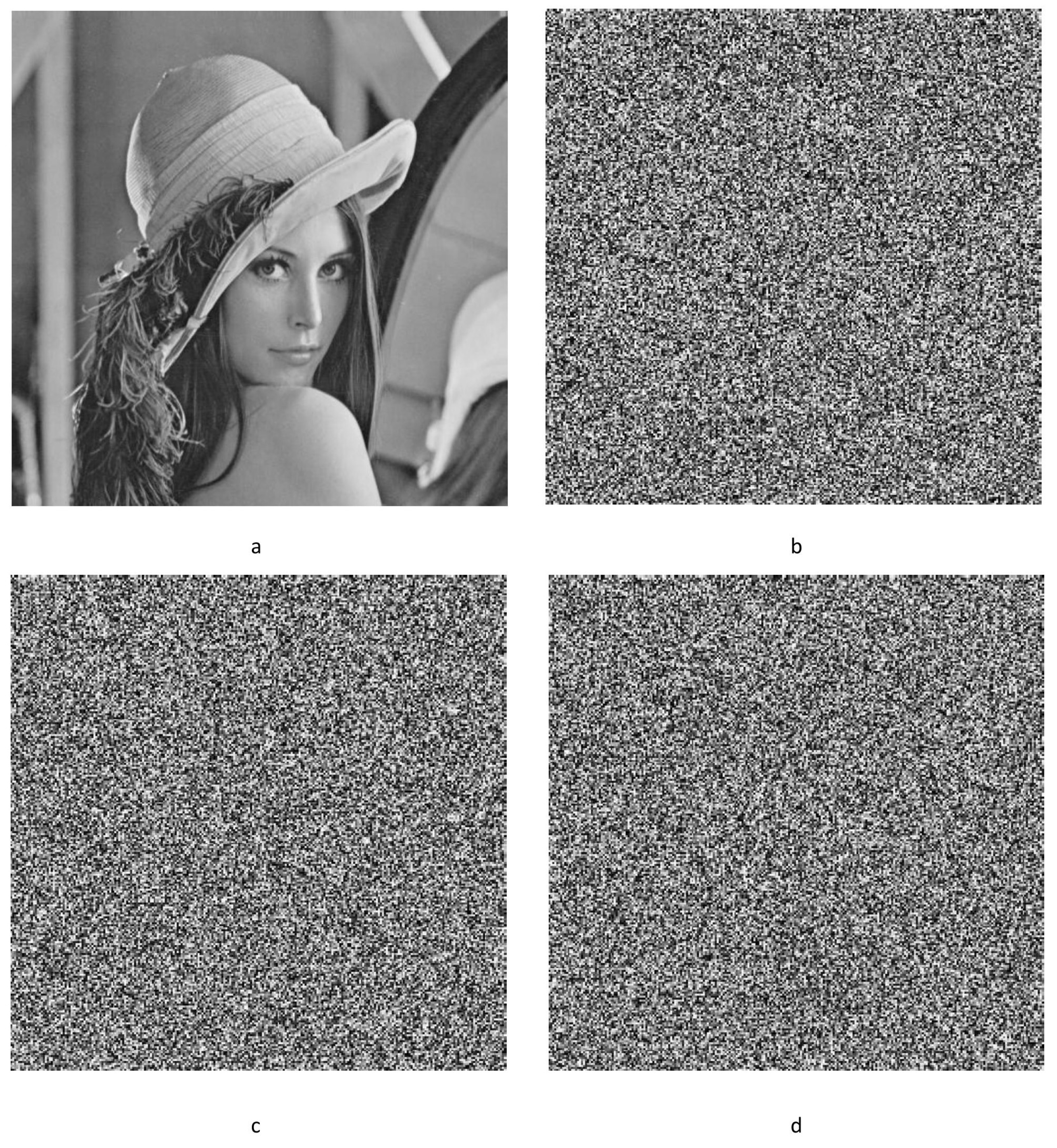
To address the disadvantages of 1D chaotic maps, this paper proposed a new nonlinearly modulated chaotic model with delay. Based on this model, FL-NMLD, a new chaotic map, was proposed. Some analysis methods, such as trajectory, Lyapunov exponent, and permutation entropy are used to evaluate its chaotic performance. Simulation results demonstrated that it has a wider chaotic range, larger Lyapunov exponents, and superior ergodicity compared to existing chaotic maps.
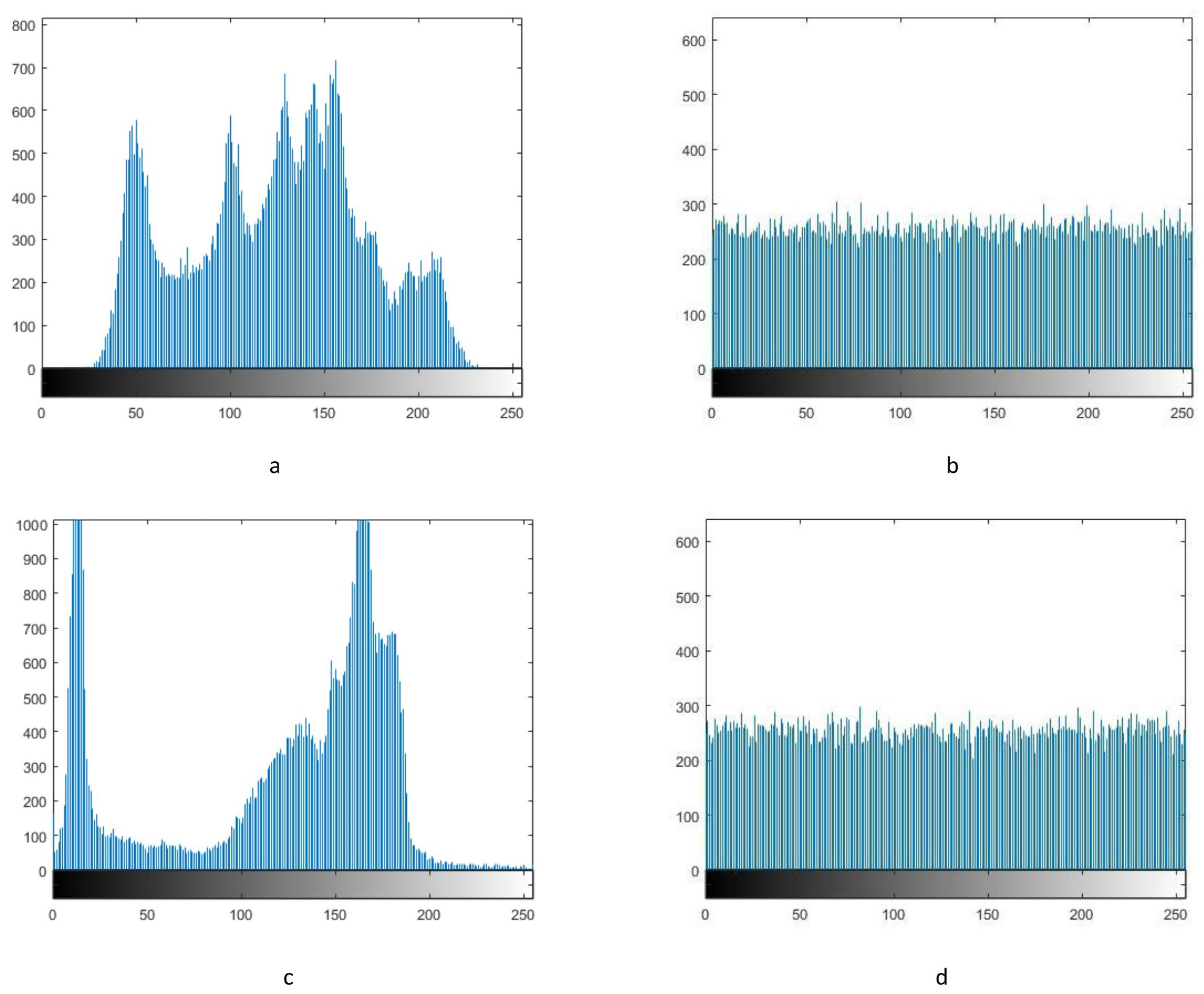
In order to apply FL-NMLD to image encryption, JPB, a new image encryption algorithm was proposed. This algorithm separate the higher four-bit planes to perform bit-plane shuffle and reassemble the lower four-bit planes into a pixel plane for pixel-plane shuffle. Experimental results show that JPB can resist most attacks and has great security performance, and it has a lower time complexity than bit-level encryption.

Author Contributions

Conceptualization, S.L.; Methodology, S.L., and B.Y.; Validation, S.L., B.Y., and W.D.; Formal Analysis, S.L.,B.Y., and W.D.; Resources, T.Z.; Data Curation, T.Z.; Writing-Original Draft Preparation, B.Y., and W.D.; Visualization, B.Y., and W.D.; Supervision, T.Z., and Y.M.; Project Administration, T.Z., and Y.M.; Funding Acquisition, T.Z., and Y.M.

Funding

This research was funded by the Fundamental Research Funds for the Central Universities (lzujbky-2018-126).

Conflicts of Interest

The authors declare no conflict of interest.

Abbreviations

The following abbreviations are used in this manuscript:
MDPIMultidisciplinary Digital Publishing Institute
DOAJDirectory of open access journals
TLAThree letter acronym
LDlinear dichroism

References

  1. Wu, Y. Image encryption using the two-dimensional logistic chaotic map. J. Electron. Imaging 2012, 21, 3014. [Google Scholar] [CrossRef]
  2. Xu, L.; Li, Z.; Li, J.; Hua, W. A novel bit-level image encryption algorithm based on chaotic maps. Opt. Lasers Eng. 2012, 78, 17–25. [Google Scholar] [CrossRef]
  3. Wang, L.; Song, H.; Liu, P. A novel hybrid color image encryption algorithm using two complex chaotic systems. Opt. Lasers Eng. 2016, 77, 118–125. [Google Scholar] [CrossRef]
  4. Wang, X.; Gu, S.; Zhang, Y. Novel image encryption algorithm based on cycle shift and chaotic system. Opt. Lasers Eng. 2015, 68, 126–134. [Google Scholar] [CrossRef]
  5. Cheddad, A.; Condell, J.; Curran, K.; Mckevitt, P. A hash-based image encryption algorithm. Opt. Commun. 2010, 283, 879–893. [Google Scholar] [CrossRef]
  6. Wang, X.; Liu, L.; Zhang, Y. A novel chaotic block image encryption algorithm based on dynamic random growth technique. Opt. Lasers Eng. 2015, 66, 10–18. [Google Scholar] [CrossRef]
  7. Rawat, N.; Kim, B.; Kumar, R. Fast digital image encryption based on compressive sensing using structurally random matrices and Arnold transform technique. Optik 2016, 127, 2282–2286. [Google Scholar] [CrossRef]
  8. Belazi, A.; El-Latif, A.A.A.; Diaconu, A.V.; Rhouma, R.; Belghith, S. Chaos-based partial image encryption scheme based on linear fractional and lifting wavelet transforms. Opt. Lasers Eng. 2017, 88, 37–50. [Google Scholar] [CrossRef]
  9. Alvarez, G.; Li, S. Cryptanalyzing a nonlinear chaotic algorithm (NCA) for image encryption. Commun. Nonlinear Sci. Numer. Simul. 2009, 14, 3743–3749. [Google Scholar] [CrossRef] [Green Version]
  10. Liu, H.; Wang, X.; Kadir, A. Image Encryption Using DNA Complementary Rule and Chaotic Maps; Elsevier Science Publishers B.V.: Amsterdam, The Netherlands, 2012; pp. 1457–1466. [Google Scholar]
  11. Zhang, Y.Q.; Wang, X.Y. A symmetric image encryption algorithm based on mixed linear-nonlinear coupled map lattice. Inf. Sci. 2014, 273, 329–351. [Google Scholar] [CrossRef]
  12. Belazi, A.; El-Latif, A.A.A.; Belghith, S. A novel image encryption scheme based on substitution-permutation network and chaos. Signal Process. 2016, 128, 155–170. [Google Scholar] [CrossRef]
  13. Arroyo, D.; Rhouma, R.; Alvarez, G.; Li, S.; Fernandez, V. On the security of a new image encryption scheme based on chaotic map lattices. Chaos Interdiscip. J. Nonlinear Sci. 2008, 18, 033112. [Google Scholar] [CrossRef] [PubMed] [Green Version]
  14. Wang, X.; Teng, L.; Qin, X. A novel colour image encryption algorithm based on chaos. Signal Process. 2012, 92, 1101–1108. [Google Scholar] [CrossRef]
  15. Arroyo, D.; Diaz, J.; Rodriguez, F.B. Cryptanalysis of a one round chaos-based Substitution Permutation Network. Signal Process. 2013, 93, 1358–1364. [Google Scholar] [CrossRef] [Green Version]
  16. Hua, Z.; Zhou, Y.; Pun, C.M.; Chen, C.L.P. 2D Sine Logistic modulation map for image encryption. Inf. Sci. Int. J. 2015, 297, 80–94. [Google Scholar] [CrossRef]
  17. Zhou, Y.; Hua, Z.; Pun, C.M.; Philip Chen, C.L. Cascade Chaotic System with Applications. IEEE Trans. Cybern. 2015, 45, 2001–2012. [Google Scholar] [CrossRef] [PubMed]
  18. Zhou, Y.; Bao, L.; Chen, C.L.P. Image encryption using a new parametric switching chaotic system. Signal Process. 2013, 93, 3039–3052. [Google Scholar] [CrossRef]
  19. Heiden, U.A.D.; Walther, H.O. Existence of chaos in control systems with delayed feedback. J. Differ. Equ. 1983, 47, 273–295. [Google Scholar] [CrossRef]
  20. Zhang, G.; Liu, Q. A novel image encryption method based on total shuffling scheme. Opt. Commun. 2011, 284, 2775–2780. [Google Scholar] [CrossRef]
  21. Liu, W.; Sun, K.; Zhu, C. A fast image encryption algorithm based on chaotic map. Opt. Lasers Eng. 2016, 84, 26–36. [Google Scholar] [CrossRef]
  22. Teng, L.; Wang, X. A bit-level image encryption algorithm based on spatiotemporal chaotic system and self-adaptive. Opt. Commun. 2012, 285, 4048–4054. [Google Scholar] [CrossRef]
  23. Gao, F.; She, S.M. Eigenvalues of non-linear equations and the Feigenbaum formula. Comput. Math. Math. Phys. 1992, 32, 403–405. [Google Scholar]
  24. Shevchenko, I.I. Lyapunov exponents in resonance multiplets. Phys. Lett. A 2014, 378, 34–42. [Google Scholar] [CrossRef] [Green Version]
  25. Bandt, C.; Pompe, B. Permutation entropy: a natural complexity measure for time series. Phys. Rev. Lett. 2002, 88, 174102. [Google Scholar] [CrossRef] [PubMed]
  26. Masoller, C.; Zanette, D.H. Anticipated synchronization in coupled chaotic maps with delays. Phys. A Stat. Mech. Its Appl. 2001, 300, 359–366. [Google Scholar] [CrossRef] [Green Version]
  27. Farmer, J.D. Chaotic attractors of an infinite-dimensional dynamical system. Phys. D Nonlinear Phenom. 1982, 4, 366–393. [Google Scholar] [CrossRef]
  28. Berre, M.L.; Ressayre, E.; Tallet, A.; Gibbs, H.M. High-dimension chaotic attractors of a nonlinear ring cavity. Phys. Rev. Lett. 1986, 56, 274–277. [Google Scholar] [CrossRef] [PubMed]
  29. Rössler, O.E. An equation for hyperchaos. Phys. Lett. A 1976, 71, 155–157. [Google Scholar] [CrossRef]
  30. Huang, X.; Ye, G. An efficient self-adaptive model for chaotic image encryption algorithm. Commun. Nonlinear Sci. Numer. Simul. 2014, 19, 4094–4104. [Google Scholar] [CrossRef]
  31. Ye, G.; Huang, X. A feedback chaotic image encryption scheme based on both bit-level and pixel-level. J. Vib. Control 2016, 22, 1171–1180. [Google Scholar] [CrossRef]
  32. Xu, L.; Gou, X.; Li, Z.; Li, J. A novel chaotic image encryption algorithm using block scrambling and dynamic index based diffusion. Opt. Lasers Eng. 2017, 91, 41–52. [Google Scholar] [CrossRef]
  33. Wu, Y.; Zhou, Y.; Saveriades, G.; Agaian, S.; Noonan, J.P.; Natarajan, P. Local Shannon entropy measure with statistical tests for image randomness. Inf. Sci. Int. J. 2013, 222, 323–342. [Google Scholar] [CrossRef] [Green Version]
  34. Wu, Y. NPCR and UACI Randomness Tests for Image Encryption. Cyber J. 2011, 1, 31–38. [Google Scholar]
  35. Farajallah, M. Chaos-Based Crypto and Joint Crypto-Compression Systems for Images and Videos. Ph.D. Thesis, Universite de Nantes, Nantes, France, 2015. [Google Scholar]
  36. Cai, S.; Huang, L.; Chen, X.; Xiong, X. A Symmetric Plaintext-Related Color Image Encryption System Based on Bit Permutation. Entropy 2018, 20, 282. [Google Scholar] [CrossRef]
  37. Wang, Y.; Wong, K.W.; Liao, X.; Chen, G. A new chaos-based fast image encryption algorithm. Appl. Soft Comput. 2011, 11, 514–522. [Google Scholar] [CrossRef]
Figure 1. NMLD model.
Electronics 07 00326 g001
Figure 2. Trajectories of (a) FL-NMLD, (b) 2D-SIMM, and (c) 2D-SLMM.
Electronics 07 00326 g002
Figure 3. Lyapunov exponents of (a) FL-NMLD, β = 0.8, (b) 2D-SLMM, and (c) 2D-SIMM, b = 5.
Electronics 07 00326 g003
Figure 4. PE α /4 ( α 1 /4, α , r−0.2, μ /4).
Electronics 07 00326 g004
Figure 5. Process of JPB image encryption.
Electronics 07 00326 g005
Figure 6. Secret key structure.
Electronics 07 00326 g006
Figure 7. Example of operations in Steps 1–3.
Electronics 07 00326 g007
Figure 8. Example of pixel-plane shuffle.
Electronics 07 00326 g008
Figure 9. Example of diffusion process.
Electronics 07 00326 g009
Figure 10. Simulation results. (ac) are original image, encrypted image, and decrypted image of Lena, respectively. (df) are original image, encrypted image, and decrypted image of Cameraman, respectively.
Electronics 07 00326 g010
Figure 11. Sensitivity test results of Lena image. (a) decrypted image with correct key. (bd) are, respectively, decrypted image adding + 10 16 to the initial values x 1 , 1 , x 1 , 2 , and the parameter α 1 .
Electronics 07 00326 g011
Figure 12. Histograms. (a,b) are histograms of Lena and its encrypted image. (c,d) are histograms of Cameraman and its encrypted image.
Electronics 07 00326 g012
Figure 13. Distributions of adjacent pixels in original image and encrypted image of Lena. (a,c,e) are distributions of original image in horizontal, vertical, and diagonal directions, respectively. (b,d,f) are distributions of encrypted image in horizontal, vertical, and diagonal directions, respectively.
Electronics 07 00326 g013
Figure 14. Values of NPCR and UACI of 150 images with one bit changed. (a) NPCR (b) UACI.
Electronics 07 00326 g014
Table 1. Information ratio of different bits in a pixel.
BitsInformation Ratio
1st0.3922%
2nd0.7843%
3rd1.5686%
4th3.1373%
5th6.2745%
6th12.5490%
7th25.0980%
8th50.1961%
Table 2. Correlation coefficients of different images.
HorizontalVerticalDiagonal
Lena0.94550.97260.9212
Encrypted Lena0.00080.00150.0032
Cameraman0.93310.95920.9074
Encrypted Cameraman0.0018−0.0032−0.0004
4.1.01.tiff0.97400.96570.9515
Encrypted 4.1.01.tiff0.00140.0014−0.0023
4.1.06.tiff0.96810.94510.9300
Encrypted 4.1.06.tiff0.00420.0022−0.0016
4.1.07.tiff0.97880.98240.9647
Encrypted 4.1.07.tiff0.00070.0041−0.0023
Table 3. Correlation coefficients of encrypted Lena using different algorithms.
HorizontalVerticalDiagonal
Lena0.94550.97260.9212
JPB0.00080.00150.0032
[16]0.0024 0.0086 0.0402
[21]0.0030−0.0024−0.0013
[2]−0.02300.0019−0.0034
[32]−0.02260.00410.0368
Table 4. Entropies of encrypted Lena using different algorithms.
Lena
JPB7.9974
[31]7.9971
[30]7.9970
[32]7.9973
[4]7.9885
Table 5. NPCR and UACI of Lena using different algorithms.
NPCRUACI
JPB99.626233.4384
[31]99.572733.4838
[30]99.592533.4275
[32]99.619233.5316
[4]99.821433.4636
Table 6. Encryption time(seconds).
256 × 256 512 × 512 Platform
JPB0.26951.1869Matlab
[2]3.134212.6917Matlab
[36]0.43891.8112Matlab
[30]0.0390.156Matlab
[37]0.00780.033C
Table 7. Comparison of encryption efficiency.
Encryption Throughput (MBps)Cycles per Byte
JPB0.231910,692.34
[2]0.047350,405.62
[36]0.142423,440.03
[30]1.60251368.76
[37]8.01369.08
Table 8. Time consumed by different processes.
ProcessTime (s)
Transform original image into the two matrices0.052
Obtain chaotic sequence for shuffle0.013
Pixel-plane shuffle0.0049
Bit-plane shuffle0.0079
Transform two shuffled matrices to obtain shuffled image0.050
Obtain and transform chaotic sequence for diffusion0.012
Diffusion0.130

