Abstract
Optimal energy extraction under partial shading conditions from a photovoltaic (PV) array is particularly challenging. Conventional techniques fail to achieve the global maximum power point (GMPP) under such conditions, while soft computing techniques have provided better results. The main contribution of this paper is to devise an algorithm to track the GMPP accurately and efficiently. For this purpose, a ten check (TC) algorithm was proposed. The effectiveness of this algorithm was tested with different shading patterns. Results were compared with the top conventional algorithm perturb and observe (P&O) and the best soft computing technique flower pollination algorithm (FPA). It was found that the proposed algorithm outperformed them. Analysis demonstrated that the devised algorithm achieved the GMPP efficiently and accurately as compared to the P&O and the FPA algorithms. Simulations were performed in MATLAB/Simulink.
1. Introduction
The depletion of fossil fuels, continuously growing energy demands, greenhouse gas (GHG) emissions, and swelling prices of fossil fuels have turned the world’s attention towards renewable and sustainable energy resources, such as solar photovoltaics (SPV) [1,2].
Transforming solar irradiance into electrical energy is the job of SPV [3]. Due to nonlinear electrical characteristics and dependence on weather conditions, the photovoltaic (PV) array cannot operate at its maximum power point (MPP). To do so, electronic trackers termed as maximum power point trackers (MPPTs) are used [4]. MPPTs are governed by different algorithms/techniques. As PV depends on weather conditions, tracking becomes difficult with changing weather conditions, especially in partial shading conditions (PSCs).
In uniform weather conditions (UWCs), all the cells of a PV array receive the same illumination, and there is only one peak in the power-voltage (P-V) curve of a PV array. Partial shading occurs when part of the PV array is shaded. This shaded part acts as a load to the unshaded part of the PV array and creates hotspots. To secure the PV array from hotspots, parallel diodes are connected across PV modules of the PV array called bypass diodes. When a PV module is shaded, it is automatically bypassed by the bypass diodes. This reduces the effect of shading at the PV array output power and prevents PV module hotspots. However, in partial shading, multiple power peaks are created in the P-V curve of the PV array due to bypass diodes. These multiple peaks are known as the local maximum power points (LMPP), except for the one with the highest power, which is called the global maximum power point (GMPP). It is very difficult to find the GMPP out of multiple LMPPs.
Conventional and soft computing (SC) MPP tracking techniques are the existing solutions for extracting maximum power from a PV array. Conventional MPPT algorithms include perturb and observe (P&O) [5], incremental conductance (InC) [6], fractional short circuit (FSC) [7], and fractional open circuit (FOC) [8]. Conventional algorithms perform efficiently in UWCs and track the MPP but with the drawbacks of oscillations of the operating power point (OPP) around the MPP and failure to perform under PSCs by sticking to the nearest LMPP [9].
Furthermore, multiple improvements have been carried out in conventional MPPT algorithms, such as the two-stage P&O [10] and direct search MPPT [11] techniques. In the first stage of the two-stage P&O technique, the optimized zone is detected, and in the second stage, the GMPP is located [10]. In the direct search MPPT technique [11], a two-mode operation is conducted. Initially, GMPP tracking mode is activated and afterwards switches to the other mode of the conventional P&O method. Improved conventional techniques are ineffective in PSCs. Overall, all of the conventional and improved conventional techniques fail to track the GMPP in PSCs. To overcome these drawbacks, researchers have considered SC techniques.
In SC techniques, the artificial neural network (ANN) [12], and fuzzy logic (FL) [13] have provided good results. However, a separate sensor arrangement is required for ANN, which increases the cost, and the FL technique needs prior system knowledge to track and requires complex fuzzy rules. These failures of ANN and FL have turned the attention of researchers towards nature-based SC techniques, such as the genetic algorithm (GA) [14], the particle swarm optimization (PSO) algorithm [15], the differential evolution (DE) algorithm [16], the random search method (RSM) [17], and the artificial bee colony (ABC) algorithm [18]. However, all of the nature-inspired SC techniques mentioned above are complex and have high computation time and low convergence speed. Still, the PSO algorithm has shown valuable improvement in tracking efficiency.
A recently introduced nature-inspired algorithm is the flower pollination algorithm (FPA) [19]. The FPA beat the most popular PSO and P&O algorithms and proved to be the top-performing technique for tracking GMPP in PSCs in [19]. The FPA shows improvement in convergence speed and efficiency. The weaknesses of FPA are its: (1) procedural complexity, (2) difficulty in parameter tuning, and (3) high computation time. FPA has fewer parameters such as switching probability and scaling factor. Nevertheless, fine tuning the switching probability is important in balancing global and local searches. Usually, the value of the switching probability has been fixed at 0.8, although this does not ensure the fine balance between the two types of searches. Such a drawback presents difficulty in GMPP tracking [20].
Research gaps in conventional techniques include: (1) removing the oscillation of the operating power point around the MPP and (2) tracking GMPP in PSCs.
Research gaps in soft computing techniques include: (1) reducing computation time, (2) increasing convergence speed, (3) reducing complexity, (4) increasing efficiency, and (5) increasing accuracy.
After considering these drawbacks, we proposed a novel method called the ten check (TC) for GMPP tracking of a PV system in PSCs. The TC algorithm has numerous notable qualities that any other conventional or soft computing technique does not have, such as: (1) parameter tuning is not required, (2) GMPP tracking is faster than any existing technique, (3) zero oscillations around MPP, and (4) GMPP is accurately and efficiently tracked.
Different patterns covering diverse weather states were tested through simulation. The results of the proposed algorithm were compared with the state-of-the-art P&O and FPA techniques. Comparisons based on tracking speed, efficiency, accuracy, parameter tuning, steady state oscillations around MPP, procedural complexity, computational complexity, and performance under PSC were made between P&O, FPA, and the proposed TC algorithm.
The TC algorithm has numerous notable qualities, which any other conventional or soft computing technique does not have, such as:
- (1)
- no parameter tuning is required,
- (2)
- track GMPP faster than any existing technique/algorithm,
- (3)
- zero oscillations around MPP,
- (4)
- track GMPP accurately and efficiently.
2. Ten Check Algorithm
2.1. Effects of Partial Shading Weather Conditions
PV cells are connected in a parallel-series arrangement to form a PV module, and in the same way, the arrangement of PV modules forms the PV array [21,22,23,24,25,26]. Under UWCs, the P-V curve of a PV array has one single MPP; however, PSCs create multiple MPPs in the P-V curve. Out of all those LMPPs, there is only one GMPP. The source of partial shading can be trees, construction, smoke, moving clouds, and bird droppings [27,28]. A PV Array of four modules with three different shaded patterns, no shading, weak partial shading, and strong partial shading is revealed in Figure 1 [29].
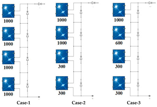
Figure 1.
Photovoltaic (PV) array with separate test cases. Case-1: zero partial shading; Case-2: weak partial shading; Case-3: strong partial shading.
In case-1 of Figure 1, there was a condition of zero shading [29]. In case-2, 50% of the PV array was shaded. Two out of four PV modules (half of the PV array) experienced the shading effect of same level (300 W/m2). This created two MPPs in the P-V curve of the PV array, one due to the top two unshaded panels and one due to the two equally shaded panels. In case-3, 75% of the PV array was shaded. Three of the four PV modules received different illuminations (1000, 600, and 300 W/m2), which created three MPPs in the P-V curve of the PV array and formed a more complex situation of GMPP tracking. Bypass diodes were used to avoid “hotspots” [30], and blocking diodes were used to stop the “reverse flow of current” [17]. One single peak was generated in the P-V curve in a uniform illumination condition and multiple peaks were generated in the P-V curve due to the number of peaks depending upon the strength of shading.
2.2. Problem Formulation
Due to the existence of multiple power peaks in the P-V curve of the PV array, an appropriate algorithm which can accurately and efficiently access the GMPP is desired. The effectiveness of the applied algorithm will affect the overall efficiency of the PV system. Bearing in mind all the above facts, the novel TC algorithm was proposed for tacking the GMPP under all weather conditions.
2.3. Ten Check Algorithm
The proposed TC algorithm smartly tackles the tracking process in 10 simple steps. Initially, 10 random samples (duty cycles) are generated in the given range of variables “A and B” (0–0.1) in the first iteration using MATLAB command rand (1, 1). (This generates uniformly distributed pseudorandom numbers drawn from the standard uniform distribution on the open interval (0, 1)). Power against each sample is calculated. The sample with highest power is saved as the “1st best” solution. In the second iteration, variables “A and B” are incremented to (0.1–0.2). The same process is repeated for the new range of variables “A and B” to get the “2nd best”. This process repeats until the number of sets reach their defined threshold value of “TEN” with variables “A and B” at “0.9–1.0”, respectively, and an array of the top 10 solutions (one solution at the end of each iteration) is obtained. The proposed TC algorithm picks the best solution from the solution array. The TC algorithm then stays with the best achieved solution and starts checking for changing weather conditions using Equations (1) and (2) [26,30]. The reinitialization of tracking process depends on the detection of changing weather. When a change is sensed, the parameters will reset automatically, and the tracking process will start again. This simple technique is equally effective in UWCs and PSCs. The TC technique is more accurate, efficient, and effective than any other existing MPPT technique. A flowchart of the TC algorithm is displayed in Figure 2.
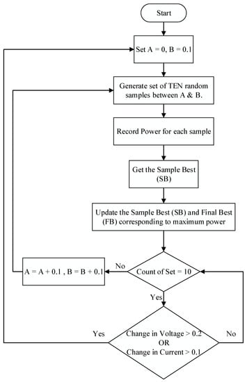
Figure 2.
Flowchart of the ten check (TC) algorithm.
Avoiding complex procedures of generating random numbers and time-wasting comparisons at each step, the TC algorithm enhances GMPP tracking speed and accuracy.
The characteristics of the PV array directly depend on weather conditions. The GMPP changes with the change in illumination and temperature; therefore, the detection of weather changes is obligatory. This change can be detected by the amount of change in voltage or current. The threshold values for the change in voltage (dV) and change in current (dI) set by the experimental trials performed in [26,27,28,29,30] are “0.2-V and 0.1 A”, respectively. These conditions are sensitive for the change of 50 W/m2. The present operating values of voltage and current are compared with their values obtained at the end of tracking process.
Vpv(t) is the voltage of a PV array at the t-th iteration and Vpv(t − 1) is the voltage of array at the preceding iteration. Ipv(t) is the current of a PV array at the t-th iteration and Ipv(t − 1) is the current of a PV array at the preceding iteration.
3. Simulation and Results
The performance evaluation and comparison of the TC algorithm with the P&O and FPA algorithms was performed in MATLAB/Simulink. The three different shading patterns discussed in Figure 1 were used for the evaluation. The system’s configuration at which the algorithms were tested was 64-bit Operating System, intel i3 Processor, and 4.00 GB RAM. The structure of the PV system with the MPPT controller is displayed in Figure 3. The TC algorithm was coded in the MATLAB/Simulink’s function block, displayed in light blue color of Figure 3. The algorithm generated a number in the range 0–1, which was injected as a duty cycle input to the DC-DC converter to change the DC voltage level. The sample time among inputs (duty cycles) was set as 0.03 s for the FPA algorithm, as mentioned in [29]. The parameter values for the P&O, FPA, and TC algorithms are presented in Table 1.
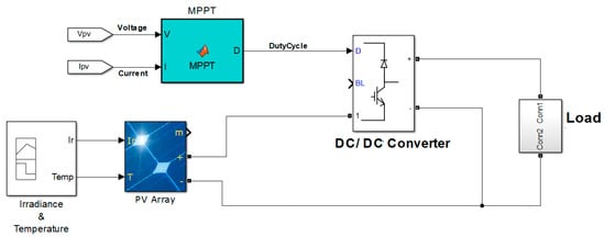
Figure 3.
Photovoltaic system’s structure.

Table 1.
Parameters of the perturb and observe (P&O), flower pollination (FPA), and TC algorithms.
3.1. Case-1: Zero Shading
In this case, where all the modules in the PV array received the same illumination and temperature, there was only one peak power point in the P-V curve. Achieving MPP here was an easy task for the P&O, FPA, and TC algorithms. The P-V and current-voltage (I-V) characteristic curves of the PV array for the zero shading condition are displayed in Figure 4.
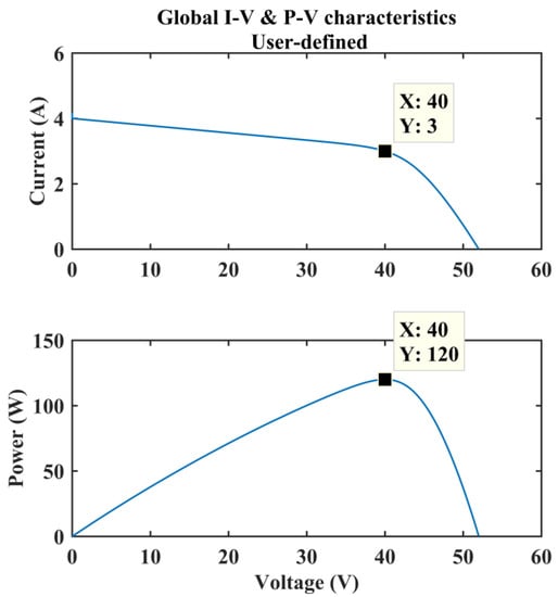
Figure 4.
Global current-voltage (I-V) and power-voltage (P-V) characteristics of a PV array in the zero shading condition.
The values of the three variables—voltage (V), current (I), and power (P)—at MPP in P-V and I-V characteristic curves displayed in Figure 4 were 40 V, 3 A, and 120 W, respectively. It can be seen in Figure 5 that the TC algorithm achieved the target of 119.7 W with 99.75% efficiency and zero oscillations, P&O extracted the full power of 120 W with 100% efficiency but with oscillations around the MPP, and FPA was successful in extracting 119.2 W with the efficiency of 99.33% and without oscillations.
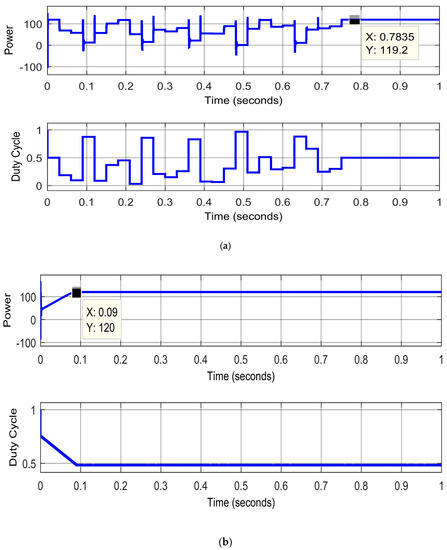
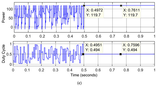
Figure 5.
Results of FPA, P&O, and TC algorithms for the zero shading condition. (a) FPA; (b) P&O; (c) TC.
Discussion of Figure 5
The extracted power and MPP tracking time of the FPA, P&O, and TC algorithms were 119.2 W in 0.75 s with an efficiency of 99.33%, 120 W in 0.09 s with an efficiency of 100%, and 119.7 W in 0.4972 s with an efficiency of 99.75%, respectively, in a uniform or zero shading condition, as displayed in Figure 5a–c. The P&O algorithm performed better but with a drawback of oscillation around MPP. The TC algorithm outperformed the FPA algorithm in all aspects and beat the P&O algorithm with zero oscillations. So, the proposed TC algorithm was the best choice, with a 99.75% efficiency and zero oscillations.
3.2. Case-2: Weak Partial Shading
In case-2 of Figure 1, weak partial shading was introduced. This created two power peaks in the P-V curve of the PV array. The P-V and I-V characteristic curves of PV array for this case are displayed in Figure 6.
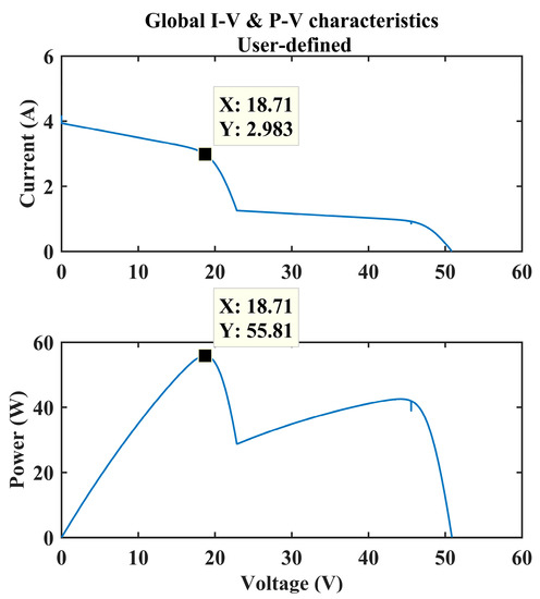
Figure 6.
Global I-V and P-V characteristics of the PV array in the weak partial shading condition.
The values of the three variables voltage (V), current (I), and power (P) at MPP in P-V and I-V characteristic curves displayed in Figure 6 were 18.71 V, 2.983 A, and 55.81 W, respectively.
Discussion of Figure 7
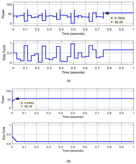
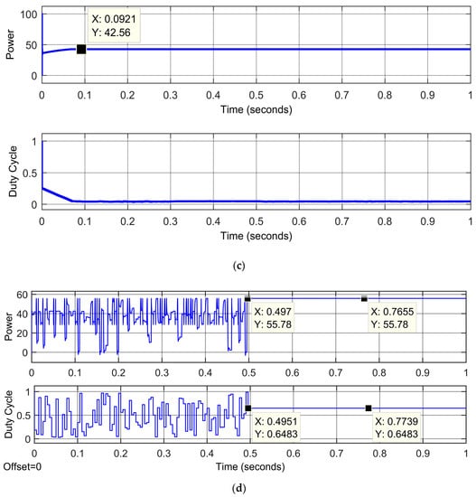
Figure 7.
Results of FPA, P&O, and TC algorithms in the weak shading condition. (a) FPA; (b) P&O (start at 0.75 duty cycle); (c) P&O (start at 0.25 duty cycle); (d) TC (tracking time and power).
The extracted power and tracking time of the FPA and the TC algorithms were 55.25 W in 0.78 s with an efficiency of 98.99% and 55.78 W in 0.497 s with an efficiency of 99.95%, respectively, in the weak partial shading condition, as displayed in Figure 7a,d. The P&O failed at tracking the GMPP because of its dependence at the starting value of the duty cycle, so it stuck to the nearest LMPP, as displayed in Figure 7b,c. It achieved 55.79 W in 0.045 s (when tracking started with duty cycle = 0.75) and achieved 42.56 W in 0.092 s (when tracking started with duty cycle = 0.25). It is evident from the results revealed in Figure 7 that the TC algorithm outperformed both the FPA and P&O algorithms in tracking time, tracking accuracy, and efficiency in the weak partial shading condition.
3.3. Case-3: Strong Shading
In case-3, strong partial shading was applied at the PV array. This created three power peaks in the P-V curve. The P-V and I-V characteristic curves of a PV array under this strong PSC are displayed in Figure 8. It is very difficult to track the GMPP in this condition.
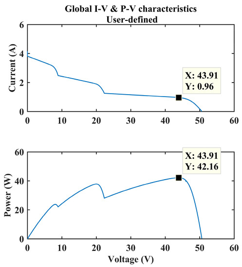
Figure 8.
Global I-V and P-V characteristics of a PV array in the strong partial shading condition.
The values of the three variables voltage (V), current (I), and power (P) at the GMPP in a P-V characteristic curve displayed in Figure 8 were 43.91 V, 0.96 A, and 42.16 W, respectively.
Discussion of Figure 9
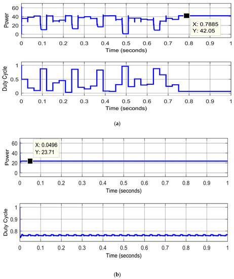
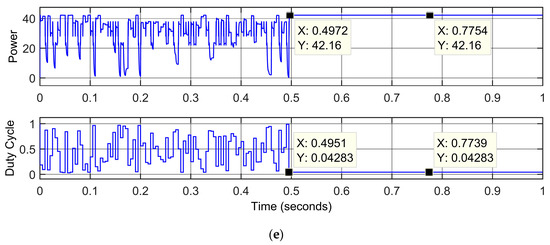
Figure 9.
Results of FPA, P&O, and TC algorithms in the strong shading condition. (a) FPA; (b) P&O (start at 0.75 duty cycle); (c) P&O (start at 0.5 duty cycle); (d) P&O (start at 0.25 duty cycle); (e) TC (tracking power confirmation).
The extracted power and tracking time of the FPA and TC algorithms were 42.05 W in 0.79 s with an efficiency of 99.74% and 42.16 W in 0.497 s with an efficiency of 100%, respectively, without oscillations in strong PSCs, as displayed in Figure 9a,d. The P&O failed at tracking the GMPP because of its dependency at the starting value of the duty cycle. It stuck to the nearest LMPP, as displayed in Figure 9b–d. It stuck to 23.71 W in 0.049 s (when tracking started with duty cycle = 0.75), it stuck to 37.69 W in 0.043 s (when tracking started with duty cycle = 0.5), and it stuck to 42.16 W in 0.32 s (when tracking started with duty cycle = 0.25). It is evident from the results presented in Figure 9 that the TC algorithm outperformed both the FPA and P&O algorithms in tracking time, tracking accuracy, and efficiency in strong PSCs.
4. Comparison
The results of the P&O, FPA, and TC algorithms for zero, partial weak, and partial strong shadings are summarized in Table 2, and the performance assessment of the TC algorithm with all the well-known algorithms published in the reputable journals is presented in Table 3.
Table 2.
Quantitative comparison between TC, FPA, and P&O algorithms.
Table 3.
Performance assessment of the TC algorithm with well-known maximum power point tracker (MPPT) algorithms.
From the summary presented in Table 2, it can be concluded that the P&O algorithm was the best choice for tracking MPP in zero shading but could not be adopted due to its failure in weak and strong partial shading conditions.
The TC algorithm beat the FPA algorithm in efficiency and tracking speed for MPP and GMPP tracking in zero, weak, and strong PSCs. Based on the performances of the TC, P&O, and FPA algorithms shown in Table 2, the TC algorithm seems to be the best choice to track MPP and GMPP in all weather conditions.
4.1. Analysis of TC for Partial Shading
The performance of the TC algorithm was checked for zero, weak, and strong PSCs, separately. Figure 10 shows the performance assessment of the TC algorithm undergoing case-1 to case-2 and then case-3 together. The rise and fall in illumination due to different actions, such as clouds, birds, falling leaves, etc., was considered and simulated, and the results are presented in Figure 10.
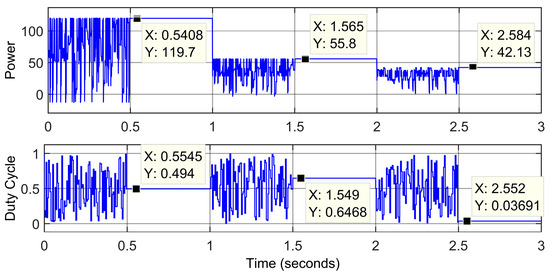
Figure 10.
Combined analysis of case-1, case-2, and case-3.
Discussion of Figure 10
The success of TC can be clearly seen in Figure 10. It started with zero partial shading (case-1); after 1 s, the PV array underwent weak partial shading (case-2), and after 2 s, the PV array experienced strong partial shading (case-3). In all the three cases, the TC algorithm retained its performance in terms of tracking time, tracking accuracy, and stability (zero oscillations). The performance analysis of the TC algorithm undergoing these three cases is summarized in Table 4.
Table 4.
Performance analysis of the TC algorithm undergoing three cases.
4.2. Uniform Shading Test
Figure 11 shows the performance assessment of the TC algorithm in UWCs. The rise and fall in illumination due to different actions, such as clouds, birds, falling leaves, etc., was considered and simulated, and the results are presented in Figure 11.
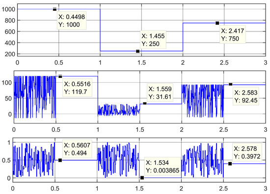
Figure 11.
Application of TC algorithm in the uniform shading condition.
Discussion of Figure 11
Figure 11 shows the simulation of the uniform shading effects. It started with zero shading, which lasted for 1 s. The TC algorithm extracted the maximum power of 119.7 W. Strong uniform shading occurred with 250 W/m2 at time 1 s, and the extracted power in this condition was 31.61 W. This fall remained for a period of 1 s and uniform shading became weak at time 2.0 s to 750 W/m2. Power of 92.45 W was tracked in this uniform weak shading. The P-V and I-V characteristic curves of the PV array for the conditions presented in Figure 11 are displayed in Figure 12.
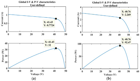
Figure 12.
I-V and P-V curves for (a) 250 and (b) 750 W/m2.
Figure 12 shows that the MPPs of the PV array at 250 and 750 W/m2 were at 32 and 92.47 W, respectively, as displayed in Figure 12a,b. Also, it is clearly displayed in Figure 4 that the MPP was at 120 W for zero shading.
The TC algorithm has achieved a power of 119.7 W in 1000 W/m2 with 99.75% efficiency, 31.61 W in 250 W/m2 with 99.78% efficiency, and 92.47 W in 750 W/m2 with 99.98% efficiency. The detailed performance analysis of the TC algorithm for uniform shading is summarized in Table 5.
Table 5.
Performance analysis the TC algorithm in the uniform shading condition.
5. More Configurations Test
Two PV arrays in parallel with each array having four PV modules in series (4S2P) is the configuration presented in cases “a” and “b” of Figure 13 for two different shading conditions. The PV arrays with six modules in series (6S) is the configuration presented in cases “c” and “d” of Figure 13 for two different shading conditions. These weather conditions were adopted from [19].
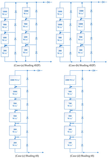
Figure 13.
Shading conditions of two configurations: 4-Series 2-Paprallel and 6-Series.
Characteristic curves for all the configurations of Figure 13 are presented in Figure 14. The values of the three variables voltage (V), current (I), and power (P) at the GMPP in the P-V and I-V characteristic curves of case-(a) are displayed in Figure 14a, which are 31.55 V, 3.87 A, and 122.1 W, respectively.
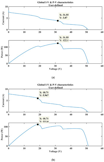
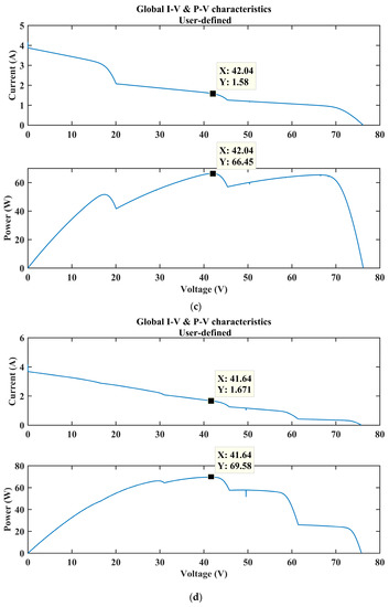
Figure 14.
Characteristic curves for all the configurations presented in Figure 13. (a) Characteristic curve for case-(a); (b) Characteristic curve for case-(b); (c) Characteristic curve for case-(c); (d) Characteristic curve for case-(d).
The values of the three variables voltage (V), current (I), and power (P) at the GMPP in P-V and I-V characteristic curves of case-b displayed in Figure 14b were 18.71 V, 5.967 A, and 111.6 W, respectively. The values of the three variables voltage (V), current (I), and power (P) at the GMPP in P-V and I-V characteristic curves of case-c displayed in Figure 14c were 42.04 V, 1.58 A, and 66.45 W, respectively. The values of the three variables voltage (V), current (I), and power (P) at the GMPP in the P-V and I-V characteristic curves of case-d displayed in Figure 14d were 41.64 V, 1.671 A, and 69.58 W, respectively.
5.1. Case-(a), Shading of 4S2P
The results of the FPA and TC algorithms for case-(a) shading 4S2P are presented in Figure 15.
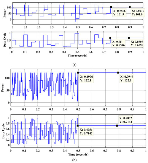
Figure 15.
Results of the FPA and TC algorithms for case-a. (a) FPA algorithm; (b) TC algorithm.
The results proved that the TC algorithm performed far better than the FPA algorithm in case-a. The FPA attained 101.9 W in 0.75 s, whereas the TC algorithm extracted 122.1 W in 0.49 s, as displayed in Figure 15a,b. The TC algorithm performed better in terms of time and tracked power.
5.2. Case-(b), Shading of 4S2P
The results of the FPA and TC algorithms for case-(b) shading 4S2P are presented in Figure 16.
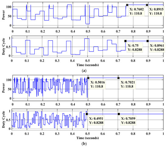
Figure 16.
Results of the FPA and TC algorithms for case-b. (a) FPA; (b) TC algorithm.
The results show that the TC algorithm extracted the same power as the FPA algorithm in case-b. Both algorithms were successful in tracking the GMPP. The FPA attained 110.8 W in 0.760 s, whereas the TC algorithm extracted 110.8 W in 0.5016 s, as displayed in Figure 16a,b. The TC algorithm performed better in terms of tracking time.
5.3. Case-(c), Shading of 6S
The results of the FPA and TC algorithms for case-(c) shading 6S are presented in Figure 17.
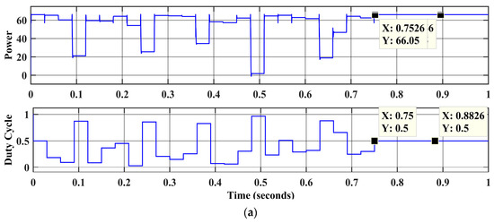
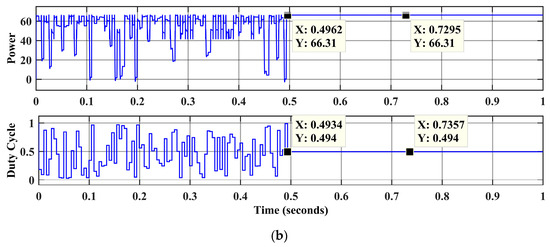
Figure 17.
Results of the FPA and TC algorithms for case-c. (a) FPA; (b) TC algorithm.
The results show that the TC algorithm outperformed the FPA algorithm in case-c. The FPA attained 66.05 W in 0.75 s, whereas the TC algorithm extracted 66.31 W in 0.4962 s, as displayed in Figure 17a,b. The TC algorithm performed better in terms of extracted power and tracking time.
5.4. Case-(d), Shading of 6S
The results of the FPA and TC algorithms for case-(d) shading 6S are presented in Figure 18.
Figure 18.
Results of the FPA and TC algorithms for case-d. (a) FPA; (b) TC algorithm.
The results show that the TC algorithm extracted the same power as the FPA algorithm in case-d. Both algorithms were successful in tracking the GMPP. The FPA attained 69.58 W in 0.751 s, whereas the TC algorithm extracted 69.58 W in 0.48 s, as displayed in Figure 18a,b. The TC algorithm performed better in terms of tracking time.
The performance of the FPA and TC algorithms for four new configurations, introduced in Figure 13, is summarized in Table 6.
Table 6.
Performance comparison between TC, FPA, and P&O algorithms.
The performance comparison of the FPA and TC algorithms for the four new configurations introduced in Figure 13 is summarized in Table 6. For the case-a “4S2P”, the TC algorithm tracked the GMPP with 100% efficiency, while the performance of the FPA algorithm was limited to 83.46%. It could not be wrong to state that the FPA algorithm failed for this condition. In terms of tracking time, the TC algorithm performed 34% faster than the FPA algorithm. For case-b of “4S2P”, the TC and FPA algorithms tracked the GMPP with 99.28% efficiency, whereas in terms of tracking time, the TC algorithm performed 34% faster than the FPA algorithm, thus making it most suitable for GMPP tracking in PSCs.
For case-c “6S”, the TC algorithm tracked the GMPP with 99.8% efficiency, while the FPA algorithm tracked the GMPP with 99.4% efficiency. The TC algorithm’s efficiency was 0.4% improved compared with the FPA algorithm. In terms of tracking time, the TC algorithm performed 34.1% faster than the FPA algorithm. For the case-d of “6S”, the TC and FPA algorithms tracked the GMPP with 100% efficiency. In terms of tracking time, the TC algorithm performed 35.7% faster than the FPA algorithm, which makes it the most suitable for GMPP tracking in PSCs.
The threshold values for the change in voltage (dV) and change in current (dI) set by the experimental trials were 0.1 V and 0.1 A and are displayed in Equations (3) and (4), respectively, for the configuration of 4S2P. The values are 0.25 V and 0.1 A and are displayed in Equations (5) and (6), respectively, for the configuration of 6S. These conditions were sensitive for the change of 50 W/m2.
6. Conclusions
A novel TC algorithm was proposed for GMPP tracking. Various cases of zero, uniform, and partial shading were simulated. These simulations and comparisons have shown the following results.
- The structure of the TC algorithm is simple and does not allow the changing weather conditions to affect its performance.
- Unlike the FPA algorithm, the TC algorithm avoids complex procedures for generating random numbers.
- Unlike the P&O algorithm, the TC algorithm does not waste time in comparing current power with the previous power at each step. These plus points have increased the tracking speed and accuracy of the TC algorithm.
- The TC algorithm achieved GMPP accurately and efficiently in all weather conditions and in record time.
Author Contributions
Generation and implementation of the idea was performed by M.M.A.A. and supervision was done by T.M.
Funding
This research received no external funding.
Acknowledgments
The authors would like to thank the research monitoring committee for their valuable comments, University of Engineering and Technology Taxila for supporting the work, and especially Malik Sher Afzal Awan for improving the quality of work with their valuable suggestions. This work was carried out in the Electrical Department, University of Engineering and Technology, Taxila, Pakistan.
Conflicts of Interest
The authors declare no conflict of interest.
Appendix A. Modeling and Characteristics of Photovoltaic Cell
Mainly, two modeling approaches exist: (1) the one/single-diode model [21] and (2) the two/double-diode model [22]. The two-diode model is more accurate, but the one-diode model is mostly used because of its simplicity [23,24]. The one/single-diode model of a PV cell is displayed in Figure A1.

Figure A1.
One-diode model of PV cell.

After applying kirchhoff’s current law, in Figure A1, the current at the output of the PV cell is:
This single-diode model has following five parameters: Ipv, ID, Rs, Rsh, and α, where Ipv = current of the PV cell, ID = diode current, Rs = resistance in series, Rsh = parallel resistance, and α = diode ideality factor VD.
The diode current can be expressed as in Equation (A2):
where VD = diode voltage, IO = reverse saturation current, and VT = thermal voltage.
The thermal voltage formula is expressed in Equation (A3):
where k = Boltzmann constant = 1.3805 × 10⁻²³, Ns = number of series connected cells, T = temperature at standard test condition (STC), and q = electron charge = 1.9 × 10⁻¹⁹ °C.
The PV array’s current can be calculated using Equation (A4):
where Npp = number of parallel connected cells, Nss = number of series connected cells, I = array current, and Ipv = array current.
The power-voltage (P-V) and current-voltage (I-V) characteristic curve is displayed in Figure A2. It can be clearly seen how the change in voltage affects the power of the PV cell. This voltage level was changed by changing the duty cycle of the DC-DC converter using MPPTs, which were governed by algorithms.

Figure A2.
Characteristic curves of PV cell for constant and changing weather conditions. (a) P-V and I-V characteristics of PV cell for uniform weather conditions. (b) I-V characteristics of PV cell with change in ambient illumination and temperature.

Figure A2a shows that the power increases for a positive change in voltage until the MPP is reached; this happens because value of the current remains constant for a changing voltage. This is a characteristic curve for a uniform illumination condition or zero shading condition. Characteristic curves for changing illumination and temperature are also presented in Figure A2b.
References
- Bastidas-Rodriguez, J.D.; Franco, E.; Petrone, G.; Ramos-Paja, C.A.; Spagnuolo, G. Maximum power point tracking architectures for photovoltaic systems in mismatching conditions: A review. IET Power Electron. 2014, 7, 1396–1413. [Google Scholar] [CrossRef]
- Ramyar, A.; Iman-Eini, H.; Farhangi, S. Global Maximum Power Point Tracking Method for Photovoltaic Arrays Under Partial Shading Conditions. IEEE Trans. Ind. Electron. 2017, 64, 2855–2864. [Google Scholar] [CrossRef]
- Stojcevski, A.; Rahim, N.A.; Chaniago, K.; Selvaraj, J. Single-phase seven-level grid-connected inverter for photovoltaic system. IEEE Trans. Ind. Electron. 2011, 58, 2435–2443. [Google Scholar]
- Bruendlinger, R.; Bletterie, B.; Milde, M.; Oldenkamp, H. Maximum power point tracking performance under partially shaded PV array conditions. In Proceedings of the 21st European Photovoltaic Solar Energy Conference and Exhibition, Dresden, Germany, 4–8 September 2006. [Google Scholar]
- Villalva, M.G.; Gazoli, J.R. Comprehensive approach to modelling and simulation of photovoltaic arrays. IEEE Trans. Power Electron. 2009, 24, 1198–1208. [Google Scholar] [CrossRef]
- Safari, A.; Mekhilef, S. Simulation and hardware implementation of incremental conductance MPPT with direct control method using Cuk converter. IEEE Trans. Ind. Electron. 2011, 58, 1154–1161. [Google Scholar] [CrossRef]
- Sher, H.A.; Murtaza, A.F.; Noman, A.; Addoweesh, K.E.; Al-Haddad, K.; Chiaberge, M. A new sensor less hybrid MPPT algorithm based on fractional short-circuit current measurement and P&O MPPT. IEEE Trans. Sustain. Energy 2015, 6, 1426–1434. [Google Scholar]
- Enslin, J.H.R.; Wolf, M.S.; Snyman, D.B.; Swiegers, W. Integrated photovoltaic maximum power point tracking converter. IEEE Trans. Ind. Electron. 1997, 44, 769–773. [Google Scholar] [CrossRef]
- Ram, J.P.; Babu, T.S.; Rajasekar, N. A comprehensive review on solar PV maximum power point tracking techniques. Renew. Sustain. Energy Rev. 2017, 67, 826–847. [Google Scholar] [CrossRef]
- Femia, N.; Petrone, G.; Spagnuolo, G.; Vitelli, M. A technique for improving P&O MPPT performances of double-stage grid-connected photovoltaic systems. IEEE Trans. Ind. Electron. 2009, 56, 3456–3467. [Google Scholar]
- Nguyen, T.L.; Low, K.S. A global maximum power point tracking scheme employing DIRECT search algorithm for photovoltaic systems. IEEE Trans. Ind. Electron. 2010, 57, 4473–4482. [Google Scholar] [CrossRef]
- Syafaruddin, E.; Hiyama, K.T. Artificial neural network-polar coordinated fuzzy controller based maximum power point tracking control under partially shaded conditions. IET Renew. Power Gener. 2009, 3, 239–253. [Google Scholar] [CrossRef]
- Chiu, C.-S.; Fuzzy, T.-S. Maximum power point tracking control of solar power generation systems. IEEE Trans. Energy Convers. 2010, 25, 1123–1132. [Google Scholar] [CrossRef]
- Mohamed, A.A.S.; Berzoy, A.; Mohammed, O. Optimized-fuzzy MPPT controller using GA for stand-alone photovoltaic water pumping system. In Proceedings of the IECON 2014—40th Annual Conference of the IEEE Industrial Electronics Society, Dallas, TX, USA, 29 October–1 November 2014; pp. 2213–2218. [Google Scholar]
- Miyatake, M.; Veerachary, M. Maximum power point tracking of multiple photovoltaic arrays: APSO approach. IEEE Trans. Aerosp. Electron. Syst. 2011, 47, 367–380. [Google Scholar] [CrossRef]
- Price, K.V.; Storn, R.M.; Lampinen, J.A. Differential Evolution: A Practical Approach to Global Optimization; Springer-Verlag: Berlin, Germany, 2005. [Google Scholar]
- Sundareswaran, K.; Peddapati, S.; Palani, S. Application of random search method for maximum power point tracking in partially shaded photovoltaic systems. IET Renew. Power Gener. 2014, 8, 670–678. [Google Scholar] [CrossRef]
- Sundareswaran, K.; Sankar, P.; Nayak, P.S.R.; Simon, S.P.; Palani, S. Enhanced Energy Output from a PV System Under Partial Shaded Conditions Through Artificial Bee Colony. IEEE Trans. Sustain. Energy 2015, 6, 198–209. [Google Scholar] [CrossRef]
- Ram, J.P.; Rajasekar, N. A new global maximum power point tracking technique for solar photovoltaic (PV) system under partial shading conditions (PSC). Energy 2017, 118, 512–525. [Google Scholar]
- Lukasik, S.; Kowalski, P.A. Study of Flower Pollination Algorithm for Continuous Optimization. In Intelligent Systems’ 2014; Springer: Cham, Switzerland, 2015; pp. 451–459. [Google Scholar]
- Koad, R.B.A.; Zobaa, A.F.; El-Shahat, A. A Novel MPPT Algorithm Based on Particle Swarm Optimization for Photovoltaic Systems. IEEE Trans. Sustain. Energy 2017, 8, 468–476. [Google Scholar] [CrossRef]
- Shongwe, S.; Hanif, M. Comparative analysis of different single-diode PV modeling methods. IEEE J. Photovolt. 2015, 5, 938–946. [Google Scholar] [CrossRef]
- Rajasekar, N.; Neeraja, K.K.; Venugopalan, R. Bacterial foraging algorithm based solar PV parameter estimation. Sol. Energy 2013, 97, 255–265. [Google Scholar] [CrossRef]
- Koran, A.; LaBella, T.; Lai, J.-S. High efficiency photovoltaic source simulator with fast response time for solar power conditioning systems evaluation. IEEE Trans. Power Electron. 2014, 29, 1285–1296. [Google Scholar] [CrossRef]
- Niranjan, D.S.; Bhaskar, D.S.; Shekar, M.J.; Sudhakar, B.T.; Rajasekar, N. Solar PV array reconfiguration under partial shading conditions for maximum power extraction using genetic algorithm. Renew. Sustain. Energy Rev. 2015, 43, 102–110. [Google Scholar]
- Rani, B.I.; Ilango, G.S.; Nagamani, C. Enhanced power generation from PV array under partial shading conditions by shade dispersion using Su Do Ku configuration. IEEE Trans. Sustain. Energy 2013, 4, 594–601. [Google Scholar] [CrossRef]
- Ishaque, K.; Salam, Z. A deterministic particle swarm optimization maximum power point tracker for photovoltaic system under partial shading condition. IEEE Trans. Ind. Electron. 2013, 60, 3195–3206. [Google Scholar] [CrossRef]
- Babu, T.S.; Rajasekar, N.; Sangeetha, K. Modified particle swarm optimization technique based maximum power point tracking for uniform and under partial shading condition. Appl. Soft Comput. 2015, 34, 613–624. [Google Scholar] [CrossRef]
- Ram, J.P.; Rajasekar, N. A Novel Flower Pollination Based Global Maximum Power Point Method for Solar Maximum Power Point Tracking. IEEE Trans. Power Electron. 2017, 32, 8486–8499. [Google Scholar]
- Sundareswaran, K.; Peddapati, S.; Palani, S. MPPT of PV systems under partial shaded conditions through a colony of flashing fireflies. IEEE Trans. Energy Convers. 2014, 29, 463–472. [Google Scholar]


© 2018 by the authors. Licensee MDPI, Basel, Switzerland. This article is an open access article distributed under the terms and conditions of the Creative Commons Attribution (CC BY) license (http://creativecommons.org/licenses/by/4.0/).