Event-Triggered and Memory-Based Sliding Mode Variable Structure Control for Memristive Systems

Abstract

This paper is concerned with a novel event-triggered sliding mode variable structure control (ESMC) scheme to achieve robust stabilization of memristive systems (MSs). First, a memory-based sliding surface, including the past and the current information of the system states, is introduced. Two switching gain matrices of such kinds of switching surfaces, which satisfy the guaranteed cost performance of the sliding reduced order dynamics, are achieved by employing linear matrix inequality techniques. Second, a sliding mode controller using an event-triggered mechanism is constructed to ensure that the trajectories of the uncertain MS slide towards the proposed memory-based switching hyperplane, and thus, the stabilization of entire MSs is reached. Finally, the effectiveness of the proposed results is demonstrated through simulations.

1. Introduction

It is well known that there are three usual fundamental circuit elements, i.e., resistors, capacitors and inductors. Now, the so-called fourth circuit element, namely the memristor, has attracted increasing attention from scientists and engineers due to its potential applications in many engineering fields, such as super-dense nonvolatile computer memories, chaotic systems, neural networks, and so on [1,2,3,4,5,6,7,8]. On the other hand, sliding mode variable structure control (SMC) has been verified to be an efficient and pretty popular robust control technique since it owns some well-known and strong properties in disturbance rejection and insensitivity to model uncertainties and parameter variations occurring in dynamical systems [9,10,11,12,13,14,15]. Many works on linear-matrix-inequality (LMI)-based SMC design, such as [16,17,18,19,20,21,22,23], form the base of LMI formulations utilized in SMC design. So far, there exists a number of results on the SMC of memristive circuits [24,25,26,27]. In the very recent paper [24], on the basis of the nonlinear Takagi–Sugeno fuzzy model, robust stabilization of uncertain memristive chaotic systems was investigated. In the literature [25], the chaotic control via a terminal SMC technique is proposed to deal with memristive oscillators, as well as Chua’s oscillators with memristors. In [26,27], the authors discussed two kinds of approaches to adaptive sliding mode synchronization for no-equilibrium memristive systems.

Recently, the mechanism of event-triggering has been regarded as one of the pretty useful and challenging techniques for control design since it can achieve control objectives with the minimum resource usage. For networked control systems [28], it also provides a beneficial way for decreasing network loads when data-packets are transmitted from different information processing terminals [29,30,31,32,33,34,35]. Meanwhile, it also turns out that the communication with the aperiodic event-triggered mechanism is quite useful, where the measurement errors play important roles in the design of the event [36,37,38,39]. In addition, the event-triggered-based SMC, developed in [40], can make the system steady-state bound be independent of both the intervals of samplings and the bounds of disturbances.

In order to reduce the costs for controlling MSs, an important way is to adopt an event-triggered scheme. However, few related results have been reported in the literature, and what is more, no results have been presented to stabilize an MS by integrating the advantages of SMC, event-triggered schemes and memory-based techniques. In this paper, the robust stabilization issue based on an ESMC scheme is investigated for MSs. The major contribution is given as follows. First, a linear time-invariant state space model is established for the Chua’s system with a memristor. Then, applying the current and the past information of MS states, a memory-based switching hyperplane is constructed, and its gains matrices, considering the guaranteed cost performance of the dynamics in the process of sliding modes, are achieved by using LMI techniques. Subsequently, an ESMC scheme is constructed such that the states of the memristive system are able to be repelled towards the desired memory-based switching manifold. Finally, robust stabilization of the entire MS is fulfilled, whose advantages and effectiveness have been verified through simulation results.

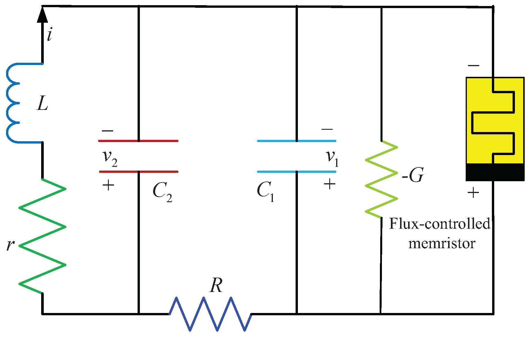
2. Description of Chua’s Circuits with Memristors

Usually, the memristor is described by the following nonlinear mathematical functions [2,3,4,41]:

$$\begin{array}{c}\hfill i=f(\varphi )v,\end{array}$$

(1)

or:

$$\begin{array}{c}\hfill v=g(q)i\end{array}$$

(2)

where $\mathrm{d}\varphi =v\mathrm{d}t$, $\mathrm{d}q=i\mathrm{d}t$, i(v) is the terminal current (voltage). The memductance $f(\varphi )$ and the memristance $g(q)$ are nonlinear functions, which are mathematically described as:

$$\begin{array}{c}\hfill \left\{\begin{array}{c}f(\varphi ):=\frac{\mathrm{d}q(\varphi )}{\mathrm{d}\varphi }\ge 0,\hfill \\ g(q):=\frac{\mathrm{d}\varphi (q)}{\mathrm{d}q}\ge 0\hfill \end{array}\right.\end{array}$$

(3)

Mathematically, $q(\varphi )$ and $\varphi (q)$ are described as the following nonlinear functions [2,3,4,41]:

$$\begin{array}{c}\hfill q(\varphi )=\left\{\begin{array}{cc}{a}_1-a_2+a_2\varphi ,\hfill & \mathrm{if}\varphi >1\hfill \\ a_1\varphi ,\hfill & \mathrm{if}-1\le \varphi \le 1\hfill \\ a_2-a_1+a_2\varphi ,\hfill & \mathrm{if}\varphi <-1\hfill \end{array}\right.\end{array}$$

(4)

and:

$$\begin{array}{c}\hfill \varphi (q)=\left\{\begin{array}{cc}{a}_3-a_4+a_{4}q,\hfill & \mathrm{if}q>1\hfill \\ a_{3}q,\hfill & \mathrm{if}-1\le q\le 1\hfill \\ a_4-a_3+a_{4}q,\hfill & \mathrm{if}q<-1\hfill \end{array}\right.\end{array}$$

(5)

where $a_i>0,$ $i=1,\cdots ,4$. They obviously have the piecewise-linear and monotone-increasing property, and one can consequently easily see that [2,4,8,24,41]:

$$\begin{array}{c}\hfill f(\varphi )=\frac{\mathrm{d}q(\varphi )}{d\varphi }=\left\{\begin{array}{cc}{a}_1,\hfill & |\varphi |\le 1,\hfill \\ a_2,\hfill & |\varphi |>1,\hfill \end{array}\right.\end{array}$$

(6)

and:

$$\begin{array}{c}\hfill g(q)=\frac{\mathrm{d}\varphi (q)}{\mathrm{d}q}=\left\{\begin{array}{cc}{a}_3,\hfill & |q|\le 1,\hfill \\ a_4,\hfill & |q|>1.\hfill \end{array}\right.\end{array}$$

(7)

Figure 1 shows a typical MS. One can briefly describe the dynamical circuit system in Figure 1 as dynamical Equation (8) according to the basic Kirchhoff circuit laws [2,4,5]:

$$\begin{array}{c}\hfill \left\{\begin{array}{ccc}{C}_1\frac{\mathrm{d}{v}_1}{\mathrm{d}t}\hfill & =& G{v}_1+\frac{v_2-v_1}{R}-f(\varphi )v_1\hfill \\ C_2\frac{\mathrm{d}{v}_2}{\mathrm{d}t}\hfill & =& \frac{v_1-v_2}{R}-i\hfill \\ L\frac{\mathrm{d}i}{\mathrm{d}t}\hfill & =& v_2-ri\hfill \\ \frac{\mathrm{d}\varphi }{\mathrm{d}t}\hfill & =& v_1\hfill \end{array}\right.\end{array}$$

(8)

As done in [42,43,44], the control input $\breve{u}(\varphi (t))$ can be added to MS (8) to solve the stabilization problem, and the system is described as:

$$\begin{array}{c}\hfill \dot{x}=\breve{A}(x)x+B\breve{u}\end{array}$$

(9)

where $x=\left[\begin{array}{c}{v}_1\\ v_2\\ i\\ \varphi \end{array}\right]$, $\breve{A}=\left[\begin{array}{cccc}\frac{GR-1-f(x_4)R}{C_{1}R}& \frac{1}{C_{1}R}& 0& 0\\ \frac{1}{C_{2}R}& -\frac{1}{C_{2}R}& -\frac{1}{C_2}& 0\\ 0& \frac{1}{L}& -\frac{r}{L}& 0\\ 1& 0& 0& 0\end{array}\right]$, $B\in R^{4\times m}$, m is the dimension of the control input.

On the basis of the mathematical Equation (6), one can arrange the MS (7) as:

$$\begin{array}{c}\hfill \dot{x}=A_{1}x+B{u}_1,\mathrm{when}|x_4|\le 1,\mathrm{or}\dot{x}=A_{2}x+B{u}_2,\mathrm{when}|x_4|>1,\end{array}$$

(10)

where $A_l=\left[\begin{array}{cccc}\frac{(G-a_l)R-1}{C_{1}R}& \frac{1}{C_{1}R}& 0& 0\\ \frac{1}{C_{2}R}& -\frac{1}{C_{2}R}& -\frac{1}{C_2}& 0\\ 0& \frac{1}{L}& -\frac{r}{L}& 0\\ 1& 0& 0& 0\end{array}\right],l=1,2.$

The system can be further represented as:

$$\begin{array}{c}\hfill \dot{x}=(A+\delta A(t))x+Bu\end{array}$$

(11)

where $A=\left[\begin{array}{cccc}\frac{(2GR-1)-(a_1+a_2)R}{2C_{1}R}& \frac{1}{C_{1}R}& 0& 0\\ \frac{1}{C_{2}R}& -\frac{1}{C_{2}R}& -\frac{1}{C_2}& 0\\ 0& \frac{1}{L}& -\frac{r}{L}& 0\\ 1& 0& 0& 0\end{array}\right]$, and $\delta A(t)$ satisfies $\delta A(t)=DF(t)E$ with $D={[1000]}^T$, $E=[\frac{a_2-a_1}{2C_1}000]$ and $F(t)=\left\{\begin{array}{c}1\mathrm{if}|x_4|\le 1\\ -1\mathrm{if}|x_4|>1\end{array}\right.$. It is obvious to see that $F(t)$ is related to the piece-wise linear characteristic caused by the memristor, and it also satisfies $|F(t)|\le 1$.

Further, $\delta A(t)$ here can also be used to describe the existing uncertainties about the values of the resistors, inductors and capacitors by selecting proper matrices D and E [24,42], and $\xi (t)$ can be modeled as the unknown bounded external disturbance.

Without lose of generality, MSs are represented by the dynamical model:

$$\begin{array}{c}\hfill \dot{x}=(A+\delta A)x+B(u+\xi ),\end{array}$$

(12)

where $x\in R^n$ is the systems state and $u\in R^m$ is the control input. $\xi \in R^m$ satisfies ${sup}_{t\ge 0}|\xi (t)|\le \overline{d}$ for all the evolution time of the memristive system, and $\overline{d}$ is a bounded and known constant.

The dynamical system (12) has the standard form by a nonsingular state transformation $x(t)=T^{-1}z(t)$,

$$\begin{array}{c}\hfill \dot{z}=(\overline{A}+\delta \overline{A})z+\overline{B}(u+\xi ),\end{array}$$

(13)

where $\left[\overline{A},\delta \overline{A}\right]=T\left[A,\delta A\right]T^{-1}$, $\overline{B}={[0{\overline{B}}_2]}^T$ with $det({\overline{B}}_2)\ne 0$.

Assumption 1.

The unknown model uncertainty $\delta \overline{A}(t)$ is time-varying mismatched and follows:

$$\begin{array}{c}\hfill \delta \overline{A}(t)=\overline{D}F(t)\overline{E},\end{array}$$

(14)

where $\overline{D}=TD$, $\overline{E}=E{T}^{-1}$ are known matrices and $F(t)$ satisfies $det(F(t))\le 1$. They are all assumed to be proper dimensions in this paper.

Let us choose the variables $z_1\in R^{n-m}$, $z_2\in R^m$, and denote $z={[z_1^T,z_2^T]}^T$, then the dynamic Equation (13) can be changed to:

$$\begin{array}{cc}\hfill \dot{z_1}& =({\overline{A}}_{11}+\delta {\overline{A}}_{11})z_1+({\overline{A}}_{12}+\delta {\overline{A}}_{12})z_2\hfill \end{array}$$

(15)

$$\begin{array}{cc}\hfill \dot{z_2}& =({\overline{A}}_{21}+\delta {\overline{A}}_{21})z_1+({\overline{A}}_{22}+\delta {\overline{A}}_{22})z_2+{\overline{B}}_2(u+\xi )\hfill \end{array}$$

(16)

where $\delta {\overline{A}}_{11}={\overline{D}}_{1}F(t){\overline{E}}_1,\delta {\overline{A}}_{12}={\overline{D}}_{1}F(t){\overline{E}}_2,\delta {\overline{A}}_{21}={\overline{D}}_{2}F(t){\overline{E}}_1$, $\delta {\overline{A}}_{22}={\overline{D}}_{2}F(t){\overline{E}}_2$, $\overline{D}={[{\overline{D}}_1^T{\overline{D}}_2^2]}^T$ and $\overline{E}=[{\overline{E}}_1{\overline{E}}_2]$. Denote:

$$\begin{array}{c}\hfill e(t)=z(t)-z(t_i),\end{array}$$

(17)

and further:

$$\begin{array}{c}\hfill e(t-d)=z(t-d)-z(t_i-d).\end{array}$$

(18)

We obviously get that $e_j(t)=z_j(t)-z_j(t_i)$ and $e_j(t-d)=z_j(t-d)-z_j(t_i-d)$, $j=1,2$.

Let $\overline{e}(t)={[e^T(t)e^T(t-d)]}^T$, and we define the event-driven mechanism in this paper as follows:

$$\begin{array}{c}\hfill |\overline{e}(t)|\le \sigma |\overline{z}(t_i)|\end{array}$$

(19)

where $\overline{z}(t_i)={[z^T(t_i),z^T(t_i-d)]}^T$ and $\sigma \in (0,1)$ is a given event-triggering constant.

The main objective in our paper is to develop the memory-based and event-driven SMC design to achieve the robust stabilization with the guaranteed cost performance index for the uncertain MS (13).

3. Main Results

3.1. Switching Hyperplane Design

According to the theory of SMC, its design includes two steps: one is to design a proper switching surface $s(t)=0$ (as we select in (20)) such that the sliding mode reduced order dynamics (as we presented in (23)) is stable with some specified control performance; the other is to develop a reaching control law for guaranteeing the reachability of $s(t)=0$ and subsequently starting the process of sliding dynamics.

In this paper, we select the following memory-based switching manifold:

$$\begin{array}{c}\hfill s(t)=z_2(t)-K{z}_1(t)-K_d{z}_1(t-d),\end{array}$$

(20)

where $K\in R^{m\times (n-m)}$ and $K_d\in R^{m\times (n-m)}$ are two gain matrices to be designed, and the memory parameter $d>0$.

Let $s(t)=0$; we have:

$$\begin{array}{c}\hfill z_2(t)=K{z}_1(t)+K_d{z}_1(t-d).\end{array}$$

(21)

Now, the reduced order system constructed by (15) and (20) can be considered as the dynamic system (15) regarding $z_1(t)$ and $z_2(t)$ in (21). As a result, the design issue of the sliding surface $s(t)$ is converted into that of the solution of the control gains K and $K_d$.

For the control gain design, we consider the following performance index:

$$\begin{array}{c}\hfill J={\int }_0^{\infty }[z_1^T(w)Q_1{z}_1(w)+z_2^T(w)R_1{z}_2(w)]dw\end{array}$$

(22)

where $Q_1$ and $R_1$ are given positive definite symmetric matrices.

Remark 1.

Such a performance index J in (22) can be regarded as the guaranteed cost performance index for MS (15) with the virtual control input $z_2$. As a consequence, how to design the sliding surface (20) with the performance index (22) is converted into the design of the control gains K, $K_d$ satisfying the so-called guaranteed cost performance index.

The purpose of selecting the memory-based switching hyperplane lies in that the control system performance index J can be improved by the added memory parameter $K_d$, and also, the dynamical system behaviors can be improved.

Now, taking $z_2(t)=K{z}_1(t)+K_d{z}_1(t-d)$ into (15), one can easily achieve the dynamics of sliding mode:

$$\begin{array}{cc}\hfill {\dot{z}}_1(t)=& {\overline{\mathbb{A}}}_1{z}_1(t)+{\overline{A}}_{12}{K}_d{z}_1(t-d)+\delta {\overline{\mathbb{A}}}_2{z}_1(t)+\delta {\overline{A}}_{12}{K}_d{z}_1(t-d)\hfill \end{array}$$

(23)

where ${\overline{\mathbb{A}}}_1={\overline{A}}_{11}+{\overline{A}}_{12}K$, $\delta {\overline{\mathbb{A}}}_2=\delta {\overline{A}}_{11}+\delta {\overline{A}}_{12}K$. Thus, the switching surface design problem is established from Theorem 1 below.

Theorem 1.

The reduced order system of the sliding mode (23) is stable and satisfies the performance index (22), if there exist matrix variables $P>0$, $Q>0$, X, Y, $K,K_d$, scalars $\alpha >0$ and $\beta >0$, such that for the given parameters $d>0$, $Q_1>0$, $R_1>0$, the matrix inequalities (24) and (25) are kept:

$$\begin{array}{c}\sum +\prod +{\prod }^T+dY<0,\hfill \end{array}$$

(24)

$$\begin{array}{c}\coprod =\Theta +\left[\begin{array}{cc}Y& 0\\ 0& 0\end{array}\right]\ge 0,\hfill \end{array}$$

(25)

where:

$$\begin{array}{c}\hfill \sum =\left[\begin{array}{cc}\sum _{11}& P{\overline{A}}_{12}{K}_d+K^T{R}_1{K}_d\\ \star & -Q+\frac{1}{\beta }{K}_d^T{\overline{E}}_2^T{\overline{E}}_2{K}_d+K_d^T{R}_1{K}_d\end{array}\right],\end{array}$$

(26)

${\sum }_{11}=(\mathrm{He}(P({\overline{A}}_{11}+{\overline{A}}_{12}K))+Q+Q_1+K^T{R}_{1}K+{({\overline{E}}_1+{\overline{E}}_{2}K)}^T\frac{1}{\alpha }({\overline{E}}_1+{\overline{E}}_{2}K))+(\alpha +\beta )P{\overline{D}}_1{\overline{D}}_1^{T}P$,

$$\begin{array}{cc}\hfill \prod & =\left[\begin{array}{cc}X& -X\end{array}\right],\hfill \\ \hfill \Theta & =\left[\begin{array}{cc}0& X\\ \star & 0\end{array}\right].\hfill \end{array}$$

(27)

Proof of Theorem 1.

During the proof process, let us choose $V(t)=V_1(t)+V_2(t)$ as the Lyapunov functional with $V_1=z_1^T(t)P{z}_1(t)$ and $V_2={\int }_{t-d}^t{z}_1^T(w)Q{z}_1(w)dw$. Now, along the state trajectory of (23), one can easily check that (28) is right by differentiating both $V_1(t)$ and $V_2(t)$ on t.

$$\begin{array}{cc}\hfill {\dot{V}}_1=& z_1^T(t)\mathrm{He}(P{\overline{\mathbb{A}}}_1+P\delta {\overline{\mathbb{A}}}_2)z_1(t)+2z_1^{T}P{\overline{A}}_{12}{K}_d{z}_1(t-d)+2z_1^{T}P\delta {\overline{A}}_{12}{K}_d{z}_1(t-d),\hfill \end{array}$$

(28)

and:

$$\begin{array}{c}\hfill {\dot{V}}_2=z_1^T(t)Q{z}_1(t)-z_1^T(t-d)Q{z}_1(t-d).\end{array}$$

(29)

Noticing that $\delta {\overline{A}}_{11}={\overline{D}}_1{F}_i(t){\overline{E}}_1$ $\delta {\overline{A}}_{12}={\overline{D}}_{1}F(t){\overline{E}}_2$ and using the mathematical basic inequality $x^{T}y+y^{T}x\le \alpha x^{T}x+\frac{1}{\alpha }{y}^{T}y$, $\alpha >0$, $x,y\in R^q$, one can obtain (30) and (31) after some calculations.

$$\begin{array}{c}2z_1^T(t)P\delta {\mathbb{A}}_2{z}_1(t)\le \alpha z_1^T(t)P{\overline{D}}_1{\overline{D}}_1^{T}P{z}_1(t)+\frac{1}{\alpha }{z}_1^T(t){\left({\overline{E}}_1+{\overline{E}}_{2}K\right)}^T\left({\overline{E}}_1+{\overline{E}}_{2}K\right)z_1(t)\hfill \end{array}$$

(30)

and:

$$\begin{array}{c}{z}_1^T(t)P\delta {\overline{A}}_{12}{K}_d{z}_1(t-d)+z_1^T(t-d)K_d^T\delta {\overline{A}}_{12}^{T}P{z}_1(t)\hfill \\ \le \beta z_1^T(t)P{\overline{D}}_1{\overline{D}}_1^{T}P{z}_1(t)+\frac{1}{\beta }{z}_1^T(t-d)K_d^T{\overline{E}}_2^T{\overline{E}}_2{K}_d{z}_1(t-d)\hfill \end{array}$$

(31)

Thanks to the relation:

$$\begin{array}{c}\hfill 2{\varpi }^T(t)X\left[{\int }_{t-d}^t{\dot{z}}_1(w)dw-z_1(t)+z_1(t-d)\right]=0\end{array}$$

(32)

where $X\in R^{2(n-m)\times (n-m)}$ and ${\varpi }^T(t)=\left[\begin{array}{cc}{z}_1^T(t),& z_1^T(t-d)\end{array}\right]$, it is not easily checked that:

$$\begin{array}{cc}\hfill \dot{V}(t)=& {\varpi }^T(t)\left(\left[\begin{array}{cc}\sum _{11}-Q_1-K^T{R}_{1}K& P{\overline{A}}_{12}{K}_d\\ \star & -Q+\frac{1}{\beta }{K}_d^T{\overline{E}}_2^T{\overline{E}}_2{K}_d\end{array}\right]+\Pi +{\Pi }^T\right)\varpi (t)\hfill \\ & -2{\varpi }^T(t)X{\int }_{t-d}^t{\dot{z}}_1(s)ds\hfill \end{array}$$

(33)

One can further obtain from the free-weight matrix ${\int }_{t-d}^t{\varpi }^T(t)Y\varpi (t)dw-d{\varpi }^T(t)Y\varpi (t)=0$ and the equation $2{\varpi }^T(t)X{\int }_{t-d}^t{\dot{z}}_1(w)dw={\int }_{t-d}^t{\eta }^T(t,w)\Theta \eta (t,w)dw$ that:

$$\begin{array}{c}\hfill \dot{V}(t)\le {\varpi }^T(t)\left(\left[\begin{array}{cc}\sum _{11}-Q_1-K^T{R}_{1}K& P{\overline{A}}_{12}{K}_d\\ \star & -Q+\frac{1}{\beta }{K}_d^T{\overline{E}}_2^T{\overline{E}}_2{K}_d\end{array}\right]+\mathrm{He}(\prod )+dY\right)\varpi (t)\end{array}$$

(34)

According to (24), this implies that:

$$\begin{array}{c}\hfill \dot{V}\le {\varpi }^T(t)\left[\begin{array}{cc}-Q_1-K^T{R}_{1}K& -K^T{R}_1{K}_d\\ \star & -K_d^T{R}_1{K}_d\end{array}\right]\varpi (t)=-z_1^T{Q}_1{z}_1-u^T{R}_{1}u<0\end{array}$$

(35)

Thus, one can see that the reduced order systems (23) is asymptotical stable. Furthermore, one can achieve the following inequality by integrating the inequality (35) from both sides in $[0,T]$:

$$\begin{array}{c}{z}_1^T(T)P{z}_1(T)-z_1^T(0)P{z}_1(0)+{\int }_{T-d}^T{z}_1^T(s)Q_1{z}_1(s)ds-{\int }_{-d}^0{z}_1^T(s)Q_1{z}_1(s)ds\hfill \\ <-{\int }_0^T{\varpi }^T(s)\left[\begin{array}{cc}{Q}_1+K^T{R}_{1}K& K^T{R}_1{K}_d\\ \star & K_d^T{R}_1{K}_d\end{array}\right]\varpi (s)ds\hfill \end{array}$$

Due to the closed-loop system being asymptotical stable, when $T\to \infty$ and $z_1(t)=0,t\in [-d,0)$, we have:

$$\begin{array}{c}\hfill J={\int }_0^{\infty }{\varpi }^T(s)\left[\begin{array}{cc}{Q}_1+K^T{R}_{1}K& K^T{R}_1{K}_d\\ \star & K_d^T{R}_1{K}_d\end{array}\right]\varpi (s)ds\le z_1^T(0)P{z}_1(0)\end{array}$$

(36)

The proof is thus completed. ☐

Based on the LMI technique, the solution to the gain matrices of the switching surface is presented in Theorem 2 below.

Theorem 2.

The sliding mode reduce order system (23) is stable with the performance index J in (22), if there exist $\mathcal{P}>0$, $\mathcal{Z}>0$, ${\mathcal{X}}_1,{\mathcal{X}}_2$, $\mathcal{Y}$, $\mathcal{K},{\mathcal{K}}_d$, scalars $\alpha >0$, $\beta >0$, such that for the given parameter $d>0$, matrices $Q_1>0$ and $R_1>0$, the following LMIs hold:

$$\begin{array}{c}\hfill \left[\begin{array}{cccccc}{\mathsf{\Omega }}_{11}& {\overline{A}}_{12}{\mathcal{K}}_d& \mathcal{P}{\overline{E}}_1^T+{\mathcal{K}}^T{\overline{E}}_2^T& 0& \mathcal{P}& \mathcal{K}\\ \star & -\mathcal{Q}& 0& {\mathcal{K}}_d^T{\overline{E}}_2& 0& {\mathcal{K}}_d^T\\ \star & \star & -\alpha I& 0& 0& 0\\ \star & \star & \star & -\beta I& 0& 0\\ \star & \star & \star & \star & -Q_1^{-1}& 0\\ \star & \star & \star & \star & \star & -R_1^{-1}\end{array}\right]\\ \hfill +H\left(\left[\begin{array}{cc}\mathrm{He}({\mathcal{X}}_1)& {\mathcal{X}}_2^T-{\mathcal{X}}_1\\ \star & -\mathrm{He}({\mathcal{X}}_2)\end{array}\right]+d\mathcal{Y}\right)H^T<0,\end{array}$$

(37)

$$\begin{array}{c}\Xi +\left[\begin{array}{cc}\mathcal{Y}& 0\\ 0& 0\end{array}\right]\ge 0,\hfill \end{array}$$

(38)

where:

$$\begin{array}{cc}\hfill {\mathsf{\Omega }}_{11}& =\mathrm{He}({\overline{A}}_{11}\mathcal{P}+{\overline{A}}_{12}\mathcal{K})+\mathcal{Q}+(\alpha +\beta ){\overline{D}}_1{\overline{D}}_1^T\hfill \end{array}$$

(39)

$$\begin{array}{cc}\hfill \Xi & =\left[\begin{array}{cc}0& \left[\begin{array}{c}{\mathcal{X}}_1\\ {\mathcal{X}}_2\end{array}\right]\\ \star & 0\end{array}\right]\hfill \\ \hfill H& =\left[\begin{array}{c}{I}_{2(n-m)}\\ 0_{(3(n-m)+2)\times (2(n-m))}\end{array}\right].\hfill \end{array}$$

(40)

In addition, the gain matrices K and $K_d$ can be achieved by:

$$\begin{array}{c}\hfill K=\mathcal{K}{\mathcal{P}}^{-1},K_d={\mathcal{K}}_d{\mathcal{P}}^{-1}.\end{array}$$

(41)

Proof of Theorem 2.

Let us multiply both sides of ∑ in (26) by $\mathrm{diag}\{P^{-1},P^{-1}\}$, and using the Schur lemma, it can be easily checked that:

$$\left[\begin{array}{cccccc}\mathrm{He}({\overline{A}}_{11}\mathcal{P}+{\overline{A}}_{12}\mathcal{K})+\mathcal{Q}+(\alpha +\beta ){\overline{D}}_1{\overline{D}}_1^T& {\overline{A}}_{12}{\mathcal{K}}_d& \mathcal{P}{\overline{E}}_1^T+{\mathcal{K}}^T{\overline{E}}_2^T& 0& \mathcal{P}& \mathcal{K}\\ \star & -\mathcal{Q}& 0& {\mathcal{K}}_d^T{\overline{E}}_2& 0& {\mathcal{K}}_d^T\\ \star & \star & -\alpha I& 0& 0& 0\\ \star & \star & \star & -\beta I& 0& 0\\ \star & \star & \star & \star & -Q_1^{-1}& 0\\ \star & \star & \star & \star & \star & -R_1^{-1}\end{array}\right]$$

(42)

where $\mathcal{P}=P^{-1}$, $\mathcal{Q}=P^{-1}Q{P}^{-1}$, $\mathcal{K}=K{P}^{-1}$ and ${\mathcal{K}}_d=K_d{P}^{-1}$.

Further, after a congruence transformation on $\Pi$ in (27) with the diagonal matrix $\mathrm{diag}\{\mathcal{P},\mathcal{P}\}$, it is easily obtained that:

$$\begin{array}{c}\mathrm{diag}\{\mathcal{P},\mathcal{P}\}\Pi \mathrm{diag}\{\mathcal{P},\mathcal{P}\}=\left[\begin{array}{cc}\left[\begin{array}{cc}\mathcal{P}& 0\end{array}\right]X\mathcal{P}& -\left[\begin{array}{cc}\mathcal{P}& 0\end{array}\right]X\mathcal{P}\\ \left[\begin{array}{cc}0& \mathcal{P}\end{array}\right]X\mathcal{P}& -\left[\begin{array}{cc}0& \mathcal{P}\end{array}\right]X\mathcal{P}\end{array}\right]\hfill \end{array}$$

(43)

Let $X=\left[\begin{array}{c}{X}_1\\ X_2\end{array}\right]$, where $X_1$, $X_2$ have the same dimension; it is easy to see that:

$$\begin{array}{c}\mathrm{diag}\{\mathcal{P},\mathcal{P}\}\mathrm{He}(\Pi )\mathrm{diag}\{\mathcal{P},\mathcal{P}\}=\left[\begin{array}{cc}\mathrm{He}({\mathcal{X}}_1)& {\mathcal{X}}_2^T-{\mathcal{X}}_1\\ \star & -\mathrm{He}({\mathcal{X}}_2)\end{array}\right]\hfill \end{array}$$

(44)

where ${\mathcal{X}}_1=\mathcal{P}{X}_1\mathcal{P}$, ${\mathcal{X}}_2=\mathcal{P}{X}_2\mathcal{P}$.

Let us denote:

$$\begin{array}{c}\hfill \mathcal{Y}=\mathrm{diag}\{\mathcal{P},\mathcal{P}\}Y\mathrm{diag}\{\mathcal{P};\mathcal{P}\}\end{array}$$

(45)

thus, by (42), (44) and (45), we have the first inequality (37).

Now, let us perform a congruence transformation on $\Theta$ by $\mathcal{S}=\mathrm{diag}\left\{\begin{array}{ccc}\mathcal{P},& \mathcal{P},& \mathcal{P}\end{array}\right\}$; one can get that:

$$\begin{array}{c}\hfill \mathcal{S}{\Theta }_i\mathcal{S}=\left[\begin{array}{cc}0& \left[\begin{array}{c}{\mathcal{X}}_1\\ {\mathcal{X}}_2\end{array}\right]\\ \star & 0\end{array}\right]=\Xi \end{array}$$

(46)

Further, by performing a congruence transformation on $\left[\begin{array}{cc}\mathcal{Y}& 0\\ 0& 0\end{array}\right]$ with $\mathcal{S}$ and noticing (45), one can convert (25) into (38).

One can thus get the conditions of stability (37) and (38). ☐

Now, the optimal control performance for sliding dynamics with the performance index (22) can be achieved by minimizing the value of $\gamma$ subject to the LMIs (38), (48) and (49).

$$\begin{array}{c}\hfill \underset{\alpha >0,\beta >0,\mathcal{P}>0,\mathcal{Z}>0,\mathcal{K},{\mathcal{K}}_d,{\mathcal{X}}_1,{\mathcal{X}}_2,\mathcal{Y},{\mathcal{Q}}_1,{\mathcal{R}}_1}{min}\gamma \end{array}$$

(47)

subject to (38), (48) and (49).

$$\begin{array}{c}\hfill \left[\begin{array}{cccccc}{\mathsf{\Omega }}_{11}& {\overline{A}}_{12}{\mathcal{K}}_d& \mathcal{P}{\overline{E}}_1^T+{\mathcal{K}}^T{\overline{E}}_2^T& 0& \mathcal{P}& \mathcal{K}\\ \star & -\mathcal{Q}& 0& {\mathcal{K}}_d^T{\overline{E}}_2& 0& {\mathcal{K}}_d^T\\ \star & \star & -\alpha I& 0& 0& 0\\ \star & \star & \star & -\beta I& 0& 0\\ \star & \star & \star & \star & -{\mathcal{Q}}_1^{-1}& 0\\ \star & \star & \star & \star & \star & -{\mathcal{R}}_1^{-1}\end{array}\right]\\ \hfill +H\left(\left[\begin{array}{cc}\mathrm{He}({\mathcal{X}}_1)& {\mathcal{X}}_2^T-{\mathcal{X}}_1\\ \star & -\mathrm{He}({\mathcal{X}}_2)\end{array}\right]+d\mathcal{Y}\right)H^T<0,\end{array}$$

(48)

$$\begin{array}{c}\left[\begin{array}{cc}-\gamma & z_1^T(0)\\ \star & -\mathcal{P}\end{array}\right]<0.\hfill \end{array}$$

(49)

where ${\mathsf{\Omega }}_{11}=\mathrm{He}({\overline{A}}_{11}\mathcal{P}+{\overline{A}}_{12}\mathcal{K})+\mathcal{Q}+(\alpha +\beta ){\overline{D}}_1{\overline{D}}_1^T$, $H=\left[\begin{array}{c}{I}_{2(n-m)}\\ 0_{(3(n-m)+2)\times (2(n-m))}\end{array}\right]$, By solving the minimum problem (47), one can achieve that the performance index $J<z_1^T(0)P{z}_1(0)<\gamma .$

3.2. The Design of Event-Based Sliding-Mode Reaching Controller

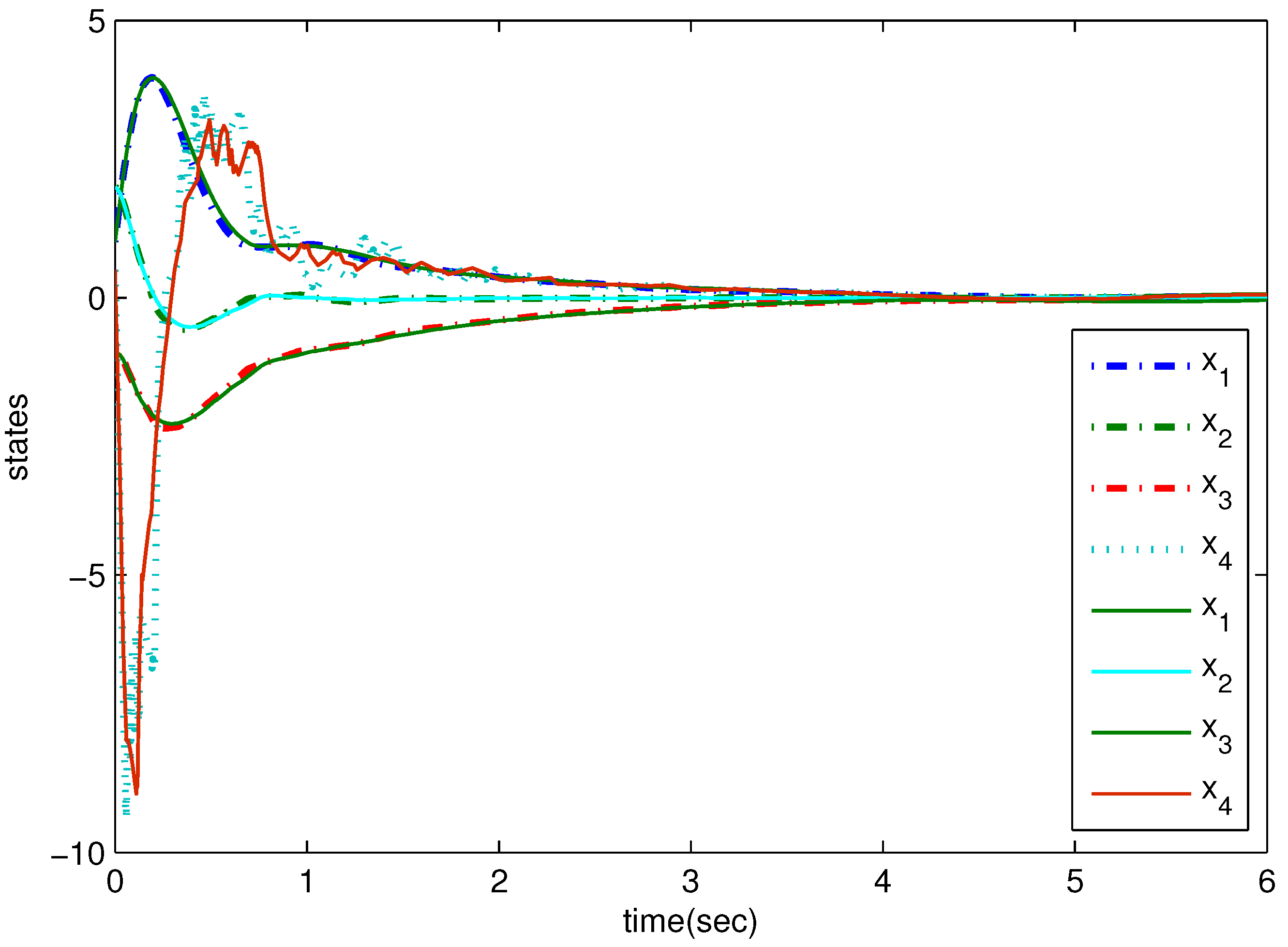
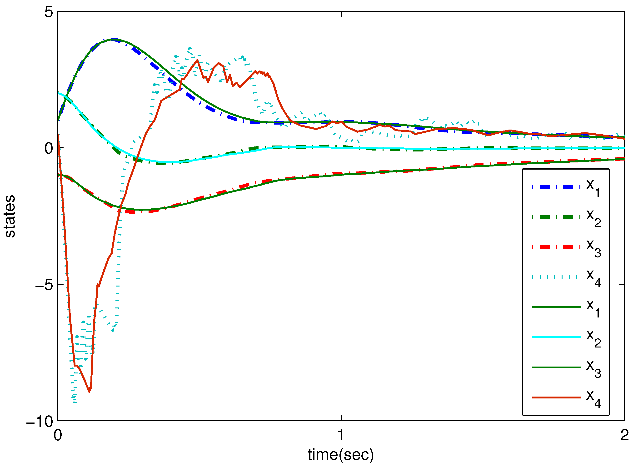
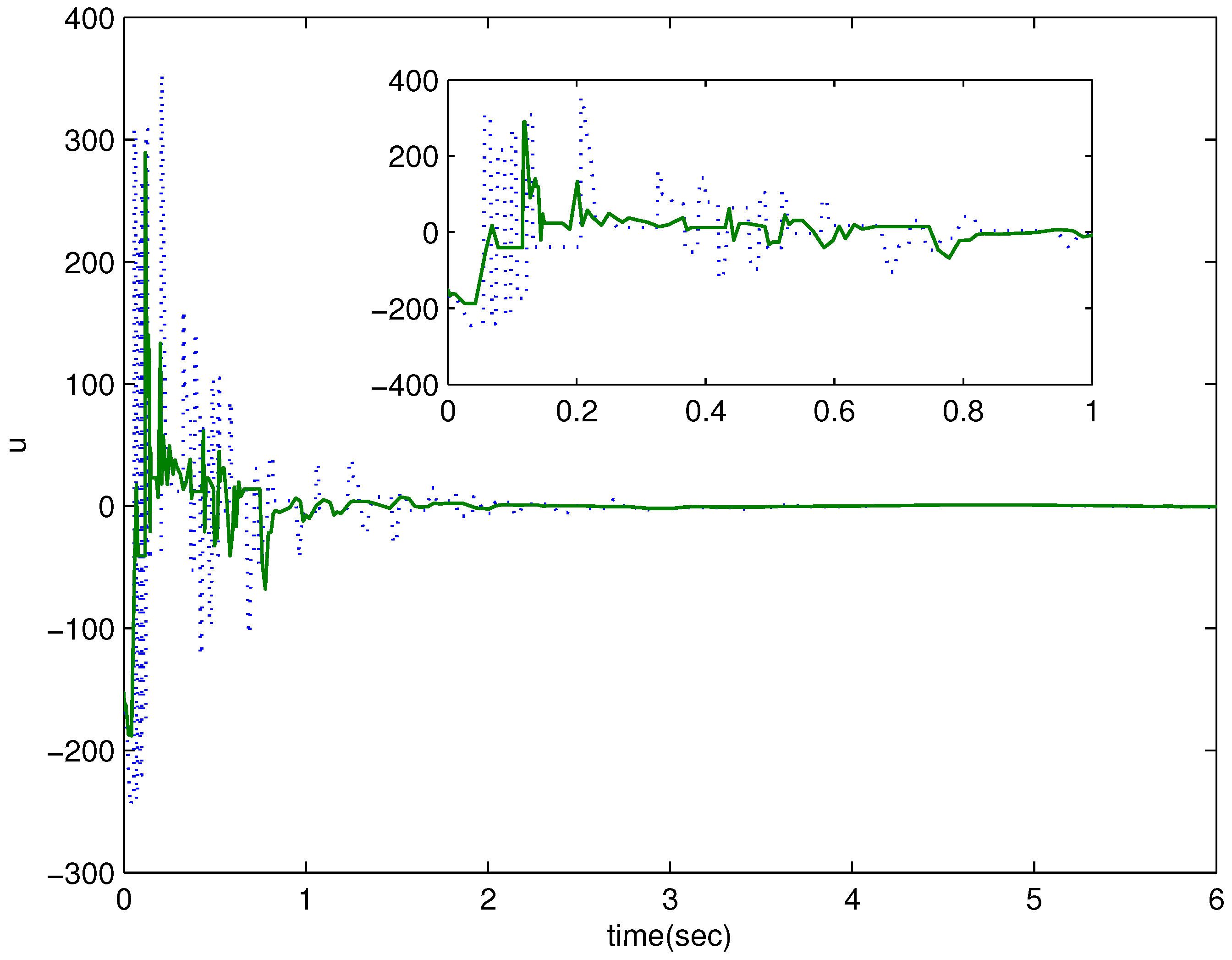
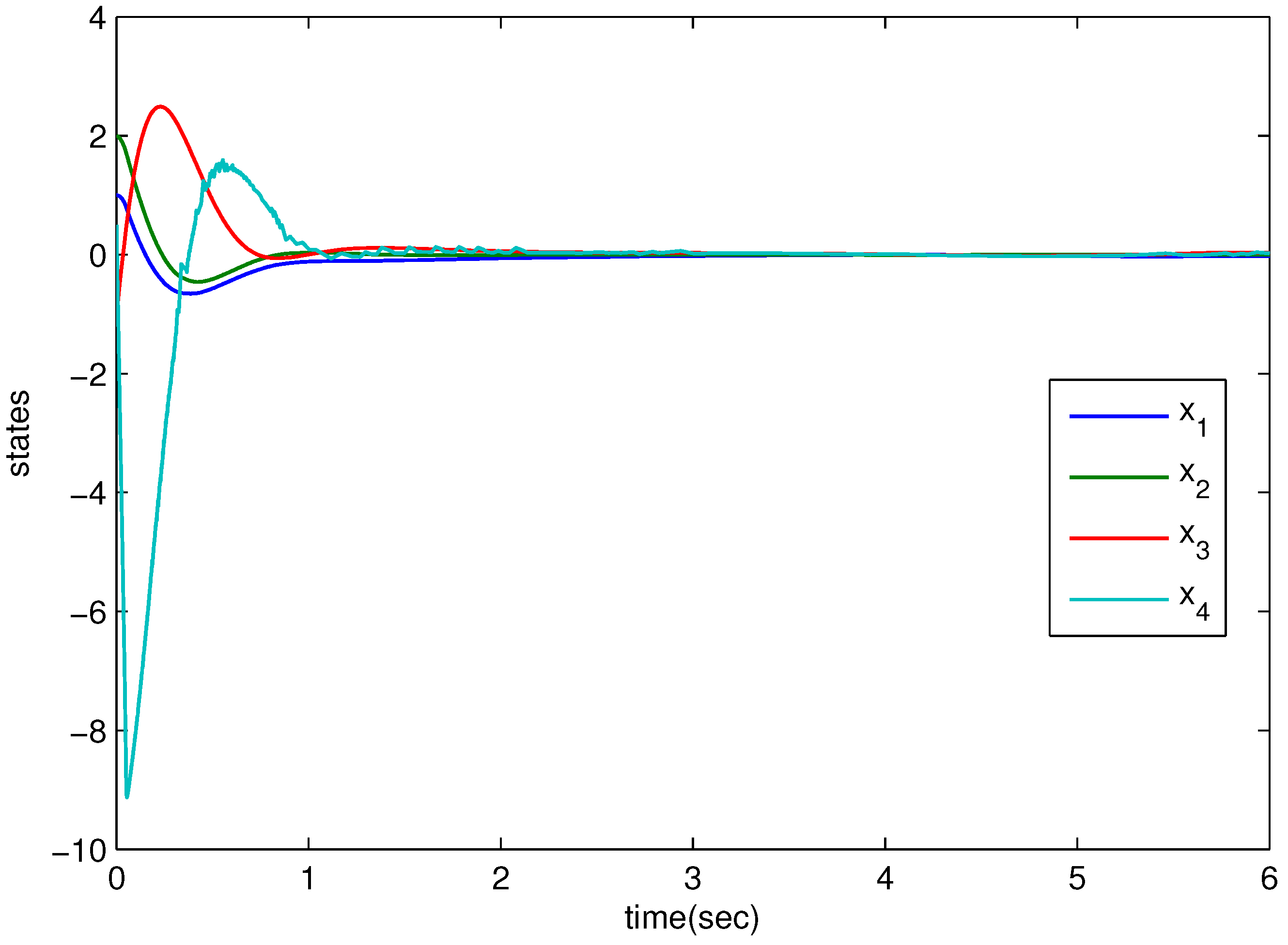
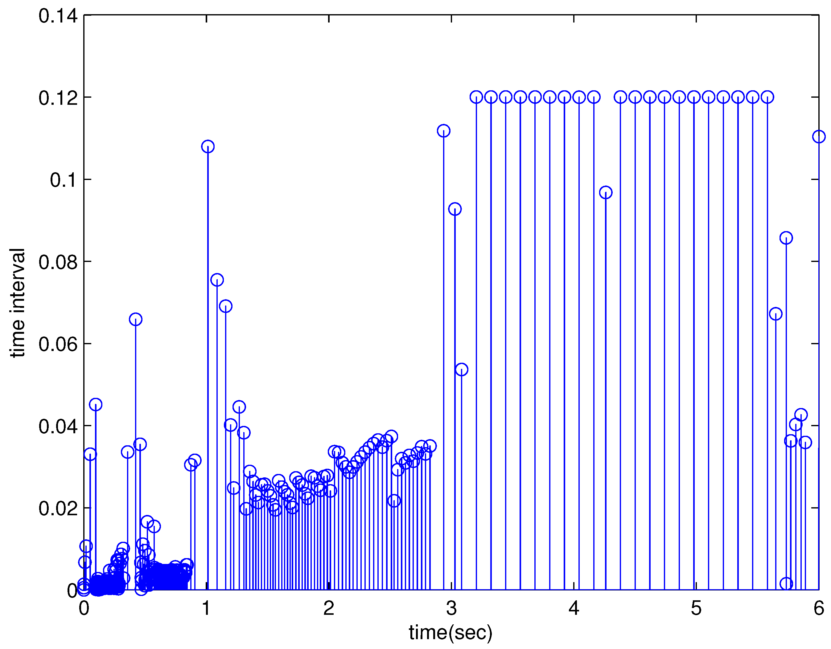
The ESMC design is presented below to ensure the arrival of the desired memory-based switching manifold (20).

Theorem 3.

State trajectories of uncertain MSs (15) and (16) can be repelled into the switching surface (20) in a limited time, when the ESMC is constructed as follows:

$$\begin{array}{cc}\hfill u(t)& =u_1(t_i)+u_2(t_i),t\in [t_i,t_{i+1})\hfill \end{array}$$

(50)

$$\begin{array}{cc}\hfill u_1(t_i)& =-{\overline{B}}_2^{-1}\left[C_1{z}_1(t_i)+C_2{z}_2(t_i)+C_3{z}_1(t_i-d)+C_4{z}_2(t_i-d)\right]\hfill \end{array}$$

(51)

$$\begin{array}{cc}\hfill u_2(t_i)& =-{\overline{B}}_2^{-1}\rho (|z(t_i)|,|z(t_i-d)|)sign(s(t_i))\hfill \end{array}$$

(52)

where:

$$\begin{array}{c}\rho (|z(t_i)|,|z(t_i-d)|)\hfill \\ =\left\{\begin{array}{cc}|{\overline{B}}_2|\overline{d}+\left(\sigma (|C|+\mathrm{Y})+\mathrm{Y}\right)(|z(t_i)|+|z(t_i-d)|)+\mu & sign(s(t))=sign(s(t_i))\\ -|{\overline{B}}_2|\overline{d}-\left(\sigma (|C|+\mathrm{Y})+\mathrm{Y}\right)(|z(t_i)|+|z(t_i-d)|)-\mu & sign(s(t))\ne sign(s(t_i))\end{array}\right.\hfill \end{array}$$

(53)

$C=[C_1,C_2,C_3,C_4]$, $C_1={\overline{A}}_{21}-K{\overline{A}}_{11}$, $C_2={\overline{A}}_{22}-K{\overline{A}}_{12}$, $C_3=-K_d{\overline{A}}_{11}$; $C_4=-K_d{\overline{A}}_{12}$; $\mathrm{Y}={\mathrm{Y}}_1+{\mathrm{Y}}_2+{\mathrm{Y}}_3+{\mathrm{Y}}_4$; ${\mathrm{Y}}_1=|D_2||E_1|+|K||D_1||E_1|$, ${\mathrm{Y}}_2=|D_2||E_2|+|K||D_1||E_2|$; ${\mathrm{Y}}_3=|K_d||D_1||E_1|$; ${\mathrm{Y}}_4=|K_d||D_1||E_2|$; μ is an arbitrary positive scalar; and σ is defined by (19).

Proof of Theorem 3.

Let us select $V(t)=\frac{1}{2}{s}^T(t)s(t)$. As a consequence, along the state trajectories of (15) and (16), we have:

$$\begin{array}{cc}\hfill \dot{V}=& s^T(t)\{\left[({\overline{A}}_{21}-K{\overline{A}}_{11})+(\delta {\overline{A}}_{21}-K\delta {\overline{A}}_{11})\right]z_1(t)\hfill \\ & +\left[({\overline{A}}_{22}-K{\overline{A}}_{12})+(\delta {\overline{A}}_{22}-K\delta {\overline{A}}_{12})\right]z_2(t)\hfill \\ & -K_d({\overline{A}}_{11}+\delta {\overline{A}}_{11})z_1(t-d)-K_d({\overline{A}}_{12}+\delta {\overline{A}}_{12})z_2(t-d)+{\overline{B}}_2(u+\xi )\}\hfill \end{array}$$

(54)

Substituting (50)–(52) into (54) and using the relations (17) and (18), then one can check by some calculations:

$$\begin{array}{cc}\hfill \dot{V}(t)=& s^T(t)\{C_1{e}_1(t)+C_2{e}_2(t)+C_3{e}_1(t-d)+C_4{e}_2(t-d)+[(\delta {\overline{A}}_{21}-K\delta {\overline{A}}_{11})e_1(t)\hfill \\ & +(\delta {\overline{A}}_{22}-K\delta {\overline{A}}_{12})e_2(t)]-\left[K_d\delta {\overline{A}}_{11}{e}_1(t-d)+K_d\delta {\overline{A}}_{12}{e}_2(t-d)\right]\hfill \\ & +\left[(\delta {\overline{A}}_{21}-K\delta {\overline{A}}_{11})z_1(t_i)+(\delta {\overline{A}}_{22}-K\delta {\overline{A}}_{12})z_2(t_i)\right]\hfill \\ & -\left[K_d\delta {\overline{A}}_{11}{z}_1(t_i-d)+K_d\delta {\overline{A}}_{12}{z}_2(t_i-d)\right]+{\overline{B}}_2{u}_2(t_i)+{\overline{B}}_2\xi \}\hfill \\ \hfill =& s^T(t)\{C\overline{e}(t)+\Theta \overline{e}(t)+{\Theta }_1{z}_1(t_i)+{\Theta }_2{z}_2(t_i)+{\Theta }_3{z}_1(t_i-d)+{\Theta }_4{z}_2(t_i-d)\hfill \\ & +{\overline{B}}_2{u}_2(t_i)+{\overline{B}}_2\xi \}\hfill \end{array}$$

(55)

where $\Theta =\left[{\Theta }_1,{\Theta }_2,{\Theta }_3,{\Theta }_4\right]$, ${\Theta }_1=\delta {\overline{A}}_{21}-K\delta {\overline{A}}_{11},{\Theta }_2=\delta {\overline{A}}_{22}-K\delta {\overline{A}}_{12},{\Theta }_3=-K_d\delta {\overline{A}}_{11},{\Theta }_4=-K_d\delta {\overline{A}}_{12}$. Noticing that $\delta {\overline{A}}_{11}={\overline{D}}_{1}F(t){\overline{E}}_1,\delta {\overline{A}}_{12}={\overline{D}}_{1}F(t){\overline{E}}_2,\delta {\overline{A}}_{21}={\overline{D}}_{2}F(t){\overline{E}}_1,\delta {\overline{A}}_{22}={\overline{D}}_{2}F(t){\overline{E}}_2$ and $F(t)F^T(t)\le I$, we have:

$$\begin{array}{cc}\hfill |\Theta |& \le |{\Theta }_1|+|{\Theta }_2|+|{\Theta }_3|+|{\Theta }_4|\hfill \\ & \le |D_2||E_1|+|K||D_1||E_1|+|D_2||E_2|+|K||D_1||E_2|+|K_d||D_1||E_1|+|K_d||D_1||E_2|\hfill \\ & ={\mathrm{Y}}_1+{\mathrm{Y}}_2+{\mathrm{Y}}_3+{\mathrm{Y}}_4=\mathrm{Y}.\hfill \end{array}$$

If the system trajectories start from a region where $\mathrm{sign}(s(t_i))=\mathrm{sign}(s(t))$, then one can see by combining with (19), (51)–(53) and $|\xi |\le \overline{d}$ that:

$$\begin{array}{cc}\hfill \dot{V}(t)\le & -\mu |s(t)|\hfill \end{array}$$

(56)

If it occurs that $\mathrm{sign}(s(t_i))=\mathrm{sign}(s(t))$, one can see that from (52) and (53) that:

$$\begin{array}{cc}\hfill u_2(t_i)=& -{\overline{B}}_2^{-1}[-|{\overline{B}}_2|\overline{d}-\left(\sigma (|C|+\mathrm{Y})+\mathrm{Y}\right)(|z(t_i)|+|z(t_i-d)|)-\mu ]\mathrm{sign}(s(t_i))\hfill \\ \hfill =& {\overline{B}}_2^{-1}[|{\overline{B}}_2|\overline{d}+\left(\sigma (|C|+\mathrm{Y})+\mathrm{Y}\right)(|z(t_i)|+|z(t_i-d)|)+\mu ]\mathrm{sign}(s(t_i))\hfill \\ \hfill =& -{\overline{B}}_2^{-1}[|{\overline{B}}_2|\overline{d}+\left(\sigma (|C|+\mathrm{Y})+\mathrm{Y}\right)(|z(t_i)|+|z(t_i-d)|)+\mu ]\mathrm{sign}(s(t))\hfill \end{array}$$

(57)

Thus, by virtue of (19), (57), $|\xi |\le \overline{d}$ and $|\Theta |\le \mathrm{Y}$, it is not hard to get that:

$$\begin{array}{cc}\hfill \dot{V}(t)=& s^T(t)\}C\overline{e}(t)+\Theta \overline{e}(t)+{\Theta }_1{z}_1(t_i)+{\Theta }_2{z}_2(t_i)+{\Theta }_3{z}_1(t_i-d)+{\Theta }_4{z}_2(t_i-d)\hfill \\ & -\left[|{\overline{B}}_2|\overline{d}+\left(\sigma (|C|+\mathrm{Y})+\mathrm{Y}\right)(|z(t_i)|+|z(t_i-d)|)+\mu \right]\mathrm{sign}(s(t))+{\overline{B}}_2\xi \}\hfill \\ \hfill \le & -\mu |s(t)|\hfill \end{array}$$

(58)

As a result, one can observe that the sliding mode reachability condition is well established. ☐

Due to the inherent execution restrictions in digital processors, the event-triggering implementation time from one to another cannot result in Zeno phenomena in the execution of the MSs.

Theorem 4.

Consider the system (13). Let $\left\{t_i\right\}$ be the generated triggering instant sequence from:

$$\begin{array}{c}\hfill t_{i+1}=inf\{t:t>t_i,\sigma |\overline{z}(t_i)|\le |\overline{e}(t)|\}\end{array}$$

(59)

for any given $\sigma \in (0,1)$. $T_i$ is then given as:

$$\begin{array}{c}\hfill T_i\ge \frac{1}{2\pi }ln\left(1+\frac{2\pi \sigma |\overline{z}(t_i)|}{ϵ+\kappa (|z(t_i)|)}\right),\end{array}$$

(60)

where $\kappa (|z(t_i)|)$ and ϵ are defined as:

$$\begin{array}{cc}\hfill \kappa (|z(t_i)|):=& 2\pi |(z(t_i)|+z(t_i-d))+(1+\sigma )|{\overline{B}}_2^{-1}||\mathbb{B}|(|C|+\mathrm{Y})(|z(t_i)|+2|z(t_i-d)|+|z(t_i-2d)|)\hfill \end{array}$$

(61)

and:

$$\begin{array}{c}\hfill \pi :=|\overline{A}|+|\overline{D}||\overline{E}|,ϵ:=2|\mathbb{B}|(|{\overline{B}}_2|\overline{d}+\mu )|{\overline{B}}_2^{-1}|,\mathbb{B}=diag\{\overline{B},\overline{B}\}\end{array}$$

(62)

Proof of Theorem 4.

Consider $\Gamma =\{t\in [t_i,\infty ):|\overline{e}(t)|=0\}$. For all $t\in [t_i,t_{i+1})\backslash \Gamma$, using the relations (17) and (18), one can check after some careful calculations that:

$$\begin{array}{c}\hfill \frac{\mathrm{d}|\overline{e}(t)|}{\mathrm{d}t}\le |\mathbb{A}\overline{e}(t)+\overline{\mathbb{A}}\overline{z}(t_i)+\mathbb{B}\left[\begin{array}{c}\vartheta (t)\\ \vartheta (t-d)\end{array}\right]|\end{array}$$

(63)

where the matrices $\mathbb{A}=\mathrm{diag}\{\overline{A}+\delta \overline{A},\overline{A}+\delta \overline{A}\}$, $\overline{\mathbb{A}}=\left[\begin{array}{c}\overline{A}+\delta \overline{A}\\ \overline{A}+\delta \overline{A}\end{array}\right]$ $\overline{z}(t_i)=\left[\begin{array}{c}z(t_i)\\ z(t_i-d)\end{array}\right]$ and $\vartheta (t)=u(t)+\xi (t)$. One can further get from Assumption 1 that:

$$\frac{\mathrm{d}|\overline{e}(t)|}{\mathrm{d}t}\le 2\pi |\overline{e}(t)|+2\pi (|z(t_i)|+|z(t_i-d)|)+|\mathbb{B}|\left[|\vartheta (t)|+|\vartheta (t-d))|\right]$$

(64)

According to (50)–(52), we have:

$$|\vartheta (t)|\le |{\overline{B}}_2^{-1}|\left[(1+\sigma )(|C|+\mathrm{Y})(|z(t_i)|+|z(t_i-d)|)+\mu +\overline{d}|{\overline{B}}_2|\right]$$

and:

$$|\vartheta (t-d)|\le |{\overline{B}}_2^{-1}|\left[(1+\sigma )(|C|+\mathrm{Y})(|z(t_i-d)|+|z(t_i-2d)|)+\mu +\overline{d}|{\overline{B}}_2|\right]$$

As a consequence, it is easy to verify that:

$$\frac{\mathrm{d}|\overline{e}(t)|}{\mathrm{d}t}\le 2\pi |\overline{e}(t)|+ϵ+\kappa (|z(t_i)|)$$

(65)

Applying the method of constant variation for the ordinary differential equation with the initial condition $\overline{e}(t_i)=|e(t_i-d))|$, it is easy to achieve that the solution of (65) is:

$$|\overline{e}(t)|\le \frac{ϵ+\kappa (|z(t_i)|)}{2\pi }(e^{2\pi (t-t_i)}-1)$$

(66)

for t in the interval $[t_i,t_{i+1})$. Applying the event-triggering rule (59), one can observe that the right-hand side of (60) always has a non-zero lower boundary. ☐

4. Example

For the proposed ESMC design methodology of the linear uncertain MS, we show an example in this section to validate its effectiveness. During the MATLAB simulation, the following data are chosen: $a_1=0.3$, $a_2=0.8$, $c_1=0.1$, $c_2=1$, $R=1$, $L=1/15$, $G=1.5$, $\frac{r}{L}=0.3$. Now, suppose that the control input is added to the memristive system as done in [24,42]; thus, we have:

$$A=\left[\begin{array}{cccc}-0.5& 10& 0& 0\\ 1& -1& -1& 0\\ 0& 15& -0.3& 0\\ 1& 0& 0& 0\end{array}\right],B=\left[\begin{array}{c}1\\ 0\\ 0\\ 0\end{array}\right].$$

Taking the nonsingular transform matrix $T=\left[\begin{array}{cccc}0& 0& 1& 0\\ 0& 1& 0& 0\\ 0& 0& 0& 1\\ 1& 0& 0& 0\end{array}\right]$, we further have:

$$\overline{A}=\left[\begin{array}{cccc}-0.3& 15& 0& 0\\ -1& -1& 0& 1\\ 0& 0& 0& 1\\ 0& 10& 0& -0.5\end{array}\right],\overline{B}=\left[\begin{array}{c}0\\ 0\\ 0\\ 1\end{array}\right].$$

In the simulation, we take $\overline{D}={[-0.51-0.50.2]}^T$, $\overline{E}=[1-110.1]$, $F=0.5\sin (t)$, $\xi =0.9\cos (2t)$ and the initial state $z_0={[12-10.5]}^T$.

Taking the memory parameter $d=0.001$, one can get by solving the LMIs (47)–(49) that:

$$K=[-3.2024-2.0482-3.6933],K_d=[1.0159-1.80310.9422]$$

with the performance index $J=27.0648$. Then, the switching hyperplane is:

$$s(t)=z_2(t)-[-3.2024-2.0482-3.6933]z_1(t)-[1.0159-1.80310.9422]z_1(t-0.001).$$

Let us choose $\mu =0.1$, $\overline{d}=0.9$ and $\sigma =0.25$, the response curves of system states, the control input, switching function and event-triggered executions are given in Figure 2, Figure 3, Figure 4, Figure 5 and Figure 6, respectively. From Figure 2 and Figure 5, one can easily see that the state trajectories of MS are able to be compelled to the desired switching manifold $s(t)=0$ in a limited time, and they then asymptotically slide towards the origin; thus, the robust stabilization of the memristive system is well established. Furthermore, it is not hard to see from Figure 6 that the triggering intervals are larger than zero, and as a result, the Zeno behavior does not arise in the whole dynamical evolution of MS.

In order to show the advantage of the proposed design method in this paper, we provide some comparison results with the ESMC with traditional memoryless switching hyperplane design approach. By solving LMIs with $d=0$, one can get $K=\left[\begin{array}{ccc}-2.1849& -3.8514& -2.7581\end{array}\right]$. At the same time, the performance index $J=27.1055$, which is bigger than the $27.0648$ obtained by the proposed design method in this paper. The responding simulation results are shown in Figure 2, Figure 3, Figure 4 and Figure 5 and Figure 7. It can be observed from the state response curves that the control input response curve and the switching function response curve that better control the performance are achieved by the proposed method in this paper.

Furthermore, we also presented the corresponding simulation results with the ESMC in [24], where $s(t)=\left[\begin{array}{cccc}2.9447& 3.4825& 1.9250& 1\end{array}\right]z=0$, $\eta =0.02$ and $ϵ=|\overline{D}||\overline{E}|$. The simulation results, including the response curves of system states, the control input, the switching function and event-triggered behavior, are shown in Figure 8, Figure 9, Figure 10 and Figure 11. By comparison, one can see that though the proposed method [24] can stabilize the memristive system, it needs many more event-triggered behaviors, especially during the reaching phase of SMC.

Thus, it is verified that the proposed memory-based ESMC design method is effective in the robust stabilization of the MSs.

5. Conclusions

Based on an event-triggered technique, the robust memory-based SMC design of uncertain MSs has been presented in this paper. At first, the uncertain Chua system with memristors has been described to be a linear uncertain system based on the memristor features. A memory-based sliding surface has then been introduced, and its design has been converted into the control gain design with the guaranteed cost performance index and can be solved by solutions to a set of LMIs. Thus, the ESMC has been presented for achieving robust stabilization of MS in spite of unknown external disturbances and uncertainties. In addition, the lower boundary for the event-triggered execution time interval has been given. An example has been finally presented for showing its effectiveness via simulation.

References

1. Chua, L. Memristor-the missing circuit element. IEEE Trans. Circuits Theory 1971, 18, 507–519. [Google Scholar] [CrossRef]
2. Itoh, M.; Chua, L. Memristor oscillators. Int. J. Bifurc. Chaos 2008, 18, 3183–3206. [Google Scholar] [CrossRef]
3. El-Sayed, A.; Elsaid, A.; Nour, H.; Elsonbaty, A. Dynamical behavior, chaos control and synchronization of a memristive ADVP circuit. Commun. Nonlinear Sci. Numer. Simul. 2013, 18, 148–170. [Google Scholar] [CrossRef]
4. Joglekar, Y.N.; Wolf, S.J. The elusive memristor: Properties of basic electrical circuits. Eur. J. Phys. 2009, 30, 661–675. [Google Scholar] [CrossRef]
5. Iu, H.; Yu, D.; Fitch, A.; Sreeram, V.; Chen, H. Controlling chaos in a memristor based circuit using a Twin-T notch filter. IEEE Trans. Circuits Syst. I Regul. Pap. 2011, 58, 1337–1344. [Google Scholar] [CrossRef]
6. Zhang, X.; Han, Q.; Zeng, Z. Hierarchical type stability criteria for delayed neural networks via canonical Bessel-Legendre inequalities. IEEE Trans. Cybern. 2018, 48, 1660–1671. [Google Scholar] [CrossRef] [PubMed]
7. Wang, G.; Cui, M.; Cai, B.; Wang, X.; Hu, T. A chaotic oscillator based on HP memristor model. Math. Probl. Eng. 2015, 2015, 561901. [Google Scholar] [CrossRef]
8. Huang, J.; Li, C.; He, X. Stabilization of a memristor-based chaotic system by intermittent control and fuzzy processing, Int. J. Control Autom. Syst. 2013, 11, 643–647. [Google Scholar] [CrossRef]
9. Edwards, C.; Spurgeon, C. Sliding Mode Control: Theory and Applications; CRC Press: Boca Raton, FL, USA, 1998. [Google Scholar]
10. Yu, X.; Wang, B.; Li, X. Computer-controlled variable structure systems: The state-of-the-art. IEEE Trans. Ind. Inform. 2012, 8, 197–205. [Google Scholar] [CrossRef]
11. Ran, S.; Xue, Y.; Zheng, B.; Wang, Z. Quantized feedback fuzzy sliding mode control design via memory-based strategy. Appl. Math. Comput. 2017, 298, 283–295. [Google Scholar] [CrossRef]
12. Zhang, B.; Han, Q.; Zhang, X. Recent advances in vibration control of offshore platforms. Nonlinear Dyn. 2017, 89, 755–771. [Google Scholar] [CrossRef]
13. Zheng, B.-C.; Yu, X.; Xue, Y. Quantized feedback sliding-mode control: An event-triiggered approached. Automatica 2018, 91, 126–135. [Google Scholar] [CrossRef]
14. Xue, Y.; Zheng, B.-C.; Yu, X. Robust sliding mode control for T-S fuzzy systems via quantized state feedback IEEE Trans. Fuzzy Syst. 2018, 26, 2261–2272. [Google Scholar] [CrossRef]
15. Zheng, B.-C.; Park, J.H. Sliding mode control design for linear systems subject to quantization parameter mismatch J. Frankl. Inst. 2016, 353, 37–53. [Google Scholar] [CrossRef]
16. Edwards, C. A practical method for the design of sliding mode controllers using linear matrix inequalitie. Automatica 2004, 40, 1761–1769. [Google Scholar] [CrossRef]
17. Yan, X.-G.; Edwards, C. Nonlinear robust fault reconstruction and estimation using a sliding mode observer. Automatica 2007, 43, 1605–1614. [Google Scholar] [CrossRef]
18. Edwards, C.; Akoachere, A. Sliding-mode output feedback controller design using linear matrix inequalities. IEEE Trans. Autom. Control 2001, 46, 115–119. [Google Scholar] [CrossRef]
19. Tan, C.P.; Edwards, C. An LMI approach for designing sliding mode observers. Int. J. Control 2001, 74, 1559–1568. [Google Scholar] [CrossRef]
20. Choi, H.H. Variable structure output feedback control design for a class of uncertain dynamic systems. Automatica 2002, 38, 335–341. [Google Scholar] [CrossRef]
21. Choi, H.H. An explict formula of linear sliding surfaces for a class of uncertain dynamic systems with mismatched uncertainties. Automatica 1998, 34, 1015–1020. [Google Scholar] [CrossRef]
22. Choi, H.H. Output feedback variable structure control design with an H performance bound constraint. Automatica 2008, 44, 2403–2408. [Google Scholar] [CrossRef]
23. Zhang, B.; Han, Q.; Zhang, X. Sliding mode control with mixed current and delayed states for offshore steel jacket platform. IEEE Trans. Control Syst. Technol. 2014, 22, 1769–1783. [Google Scholar] [CrossRef]
24. Wen, S.; Huang, T.; Yu, X.; Chen, M.Z.; Zeng, Z. Sliding-mode control of memristive Chua’s systems via the event-based method. IEEE Trans. Circuits Syst. II Express Briefs 2017, 64, 81–85. [Google Scholar] [CrossRef]
25. Abolmasoumi, A.H.; Khosravinejad, S. Chaos Control in Memristor-Based Oscillators Using Intelligent Terminal Sliding Mode Controller. Int. J. Comput. Theory Eng. 2016, 8, 506–511. [Google Scholar] [CrossRef]
26. Rajagopal, K.; Bayani, A.; Khalaf, A.J.M.; Namazi, H.; Jafari, S.; Pham, V.T. A no-equilibrium memristive system with four-wing hyperchaotic atracto. Int. J. Electron. Commun. 2018, 95, 207–215. [Google Scholar] [CrossRef]
27. Rajagopal, K.; Guessas, L.; Karthikeyan, A.; Srinivasan, A.; Adam, G. Fractional order memristor no equilibrium chaotic system with its adaptive sliding mode synchronization and genetically optimized fractional order PID synchronization. Complexity 2017. [Google Scholar] [CrossRef]
28. Zhang, X.; Han, Q. Network-based H filtering using a logic jumping-like trigger. Automatica 2013, 49, 1428–1435. [Google Scholar] [CrossRef]
29. Wang, Y.-L.; Han, Q.-L.; Fei, M.; Peng, C. Network-based T-S fuzzy dynamic positioning controller design for unmanned marine vehicles. IEE Trans. Cybern. 2018, 48, 2750–2763. [Google Scholar] [CrossRef] [PubMed]
30. Wang, Y.-L.; Han, Q.-L. Network-based modelling and dynamic output feedback control for unmanned marine vehicles. Automatica 2018, 91, 43–53. [Google Scholar] [CrossRef]
31. Liu, J.; Zha, L.; Xie, X.; Tian, E. Resilient observer-based control for networked nonlinear T-S fuzzy systems with hybrid-triggered scheme. Nonlinear Dyn. 2018, 91, 2049–2061. [Google Scholar] [CrossRef]
32. Liu, J.; Xia, J.; Tian, E.; Fei, S. Hybrid-driven-based H-infinity filter design for neural networks subject to deception attacks. Appl. Math. Comput. 2018, 320, 158–174. [Google Scholar]
33. Li, H.; Liao, X.; Huang, T.; Zhu, W. Event-triggering sampling based leader-following consensus in second-order multi-agent systems. IEEE Trans. Autom. Control 2015, 60, 1998–2003. [Google Scholar] [CrossRef]
34. Zhang, X.-M.; Han, Q.-L. Event-triggered H control for a class of nonlinear networked control systems using novel integral inequalities. Int. J. Robust Nonlinear Control 2017, 27, 679–700. [Google Scholar] [CrossRef]
35. Zhang, X.-M.; Han, Q.-L. A decentralized event-triggered dissipative control scheme for systems with multiple sensors to sample the system outputs. IEEE Trans. Cybern. 2016, 46, 2745–2757. [Google Scholar] [CrossRef] [PubMed]
36. Zhou, B.; Liao, X.; Huang, T.; Chen, G. Leader-following exponential consensus of general linear multi-agent systems via event-triggered control with combinational measurements. Appl. Math. Lett. 2015, 40, 35–39. [Google Scholar] [CrossRef]
37. Wen, S.; Huang, T.; Yu, X.; Chen, M.Z.; Zeng, Z. Aperiodic sampled-data sliding-mode control of fuzzy systems with communication delays via the event-triggered method. IEEE Trans. Fuzzy Syst. 2016, 24, 1048–1057. [Google Scholar] [CrossRef]
38. Zhang, B.; Han, Q.; Zhang, X. Event-triggered H control for offshore structures in network environments. J. Sound Vib. 2016, 368, 1–21. [Google Scholar] [CrossRef]
39. Wang, J.; Zhang, X.; Han, Q. Event-triggered generalized dissipativity filtering for neural networks with time-varying delays. IEEE Trans. Neural Netw. Learn. Syst. 2016, 27, 77–88. [Google Scholar] [CrossRef] [PubMed]
40. Behera, A.; Bandyopadhyay, B. Robust sliding mode control: An event-triggering approach. IEEE Trans. Circuits Syst. II Express Briefs 2017, 64, 146–150. [Google Scholar] [CrossRef]
41. Petras, I. Fractional-order memristor-based Chua’s circuit. IEEE Trans. Circuits Syst. II Express Briefs 2010, 57, 975–979. [Google Scholar] [CrossRef]
42. Wen, S.; Zeng, Z.; Huang, T. Event-based control for memristive systems. Commun. Nonlinear Sci. Numer. Simul. 2014, 19, 3431–3443. [Google Scholar] [CrossRef]
43. Kocamaz, U.E.; Cevher, B.; Uyaroǧlu, Y. Control and synchronization of chaos with sliding mode control based on cubic reaching rule. Chaos Solitons Fractals 2017, 105, 92–98. [Google Scholar] [CrossRef]
44. Ablay, G. Sliding mode control of uncertain unified chaotic systems. Nonlinear Anal. Hybrid Syst. 2009, 3, 531–535. [Google Scholar] [CrossRef]
Figure 1. Memristive systems.
Electronics 07 00253 g001
Figure 2. The system states’ evolution curves (the proposed method with solid lines, the memoryless design method with dashed lines).
Electronics 07 00253 g002
Figure 3. The system states’ evolution curves (the proposed method with solid lines, the memoryless design method with dashed lines).
Electronics 07 00253 g003
Figure 4. The control input evolution curves (the proposed method with solid lines, the memoryless design method with dashed lines).
Electronics 07 00253 g004
Figure 5. The switching function response curves (the proposed method with solid lines, the memoryless design method with dashed lines).
Electronics 07 00253 g005
Figure 6. Evolution of the execution time interval (the proposed design method).
Electronics 07 00253 g006
Figure 7. Evolution of the execution time interval (the memoryless design method).
Electronics 07 00253 g007
Figure 8. The system states’ evolution curves.
Electronics 07 00253 g008
Figure 9. The control input evolution curve.
Electronics 07 00253 g009
Figure 10. The switching function response curve.
Electronics 07 00253 g010
Figure 11. Evolution of the execution time interval.
Electronics 07 00253 g011