Abstract
In this paper, we propose a simple approach for sparse array synthesis. We employ a modified generalized alternate projection algorithm using -norm constrained minimization in order to achieve the excitation and the position of the elements of a sparse array. The proposed approach is very flexible, since it deals with power pattern masks and allows the inclusion of the effects of element pattern and mutual coupling. Its implementation is relatively simple, thanks to the possibility to use well-known convex programming techniques. The presented method is particularly suitable for the synthesis of patterns commonly employed in radar systems; the numerical results provided show good performances with respect to concurrent methods available in open literature.
1. Introduction
Array pattern synthesis is of paramount importance for designing modern radar systems, and it is an important and active area of research. Particularly attractive is the use of non-equispaced (or sparse) arrays, by means of which it is possible to reduce the overall number of radiating elements without a significant degradation of the performances with respect to half-wavelength equispaced arrays.
Many efficient synthesis strategies are available in the case of fixed positions of the radiating elements [1,2]. These algorithms take advantage of the linear relationship between the far-field and the unknown (i.e., the excitations of the radiating elements), and, with proper constraints, require the use of fast and efficient local minimizing algorithms.
On the contrary, the efficient synthesis of non-equispaced (or sparse) arrays is an open problem. In fact, the strong nonlinearity of the radiation operator with respect to the array elements’ positions prevents the effectiveness of local minimization algorithms. The use of global minimizing approaches, like evolutionary algorithms, allows to asymptotically obtain an optimal solution of the problem. In spite of the use of hybrid techniques that adopt local minimizers for the convex part of the problem, a strong computational effort is required, in particular when the number of unknowns becomes large. In fact, for a given precision, the computational burden grows exponentially with the number of unknowns [3].
Besides the use of evolutionary or hybrid algorithms, a number of fast deterministic synthesis techniques, based on the discretization of the current distribution obtained in case of continuous source, have been developed in the last few decades [4,5,6].
Usually in these approaches, the number of radiating elements is fixed, while their positions and excitation coefficients are the output of the synthesis procedure. As a matter of fact, a number of trials is required to identify the minimum number of radiating elements. Consequently, an algorithm able to give the positions, the excitation and the number of radiating elements of the sparse array are of interest.
From a mathematical point of view, we need to identify the (hopefully) sparsest excitation providing a pattern verifying the required specifications in terms of main lobe, side-lobe levels, gain and so on. In the last decade, some dramatic advances have been obtained in the field of Sparse Recovery (SR), mainly pushed by the huge interest toward the Compressed Sensing (CS) theory. Basically, SR and CS deal with sparse vectors, i.e., vectors having a large number of null (or almost null) elements. The success of SR and CS is due to the availability of efficient algorithms able to solve undetermined linear systems involving sparse unknowns, like the minimization. Basically, the minimization promotes the sparsification of the unknown vector [7,8,9,10].
Based on this behaviour, a number of researchers [11,12,13] have recently used compressive sensing to promote sparsification in array synthesis.
Most of the current implementations of sparse-forcing algorithms in array synthesis problems find a sparse source that mimics a specific pattern, obtained with standard equispaced arrays synthesis techniques. Since the sparse array found by means of these approaches will radiate a pattern that is just an approximation of the specific one chosen, the specifications of the achieved layout could also be an approximation of the desired ones, and the actual performances can be known only a posteriori.
The approach described in this paper overcomes this issue by introducing a new algorithm, the Sparse-Forcing Generalized Alternate Projection (SFGAP). This algorithm is a significant improvement with respect to the CSGAP (Compressive Sensing Generalized Alternate Projections) presented in [14], and employs a modified generalized alternate projection algorithm [15] using norm minimization in order to achieve the excitation and the position of the elements of a sparse array satisfying the synthesis constraints imposed by a power pattern mask. It is worth noting that the use of alternating algorithms, together with minimization, has been shown to provide very good results in fields different from antenna array synthesis [16,17].
In the next section, before the discussion of the SFGAP, we would like to present the less general case of the synthesis of sparse arrays with arbitrary upper masks, by means of minimization: some of the results we will find are exploited to achieve the SFGAP.
2. Sparse Array Synthesis with Arbitrary Upper Masks
In this paragraph, we will preliminarily discuss the synthesis of sparse arrays with arbitrary upper masks; without loss of generality, we will focus on pencil beam patterns.
The sparse array synthesis can be formulated as:
where N is the number of radiators, is the vector of their positions, is the vector of their relative excitations, is an arbitrary upper mask, is the maximum size of the linear array, and
is the array factor of the sparse array, with , θ being the angular direction with respect to broadside, and β the free-space wavenumber.
Let us now introduce a dense equispaced position ν-element vector in the range , with a spacing δ much smaller than , for instance , where λ is the free-space wavelength. Let be the excitation of such a dense array, and a μ-element vector sampling the u range in which the mask specifications are given; the radiation operator can be expressed as the matrix such that
where is the sampled array factor.
According to the introduced notation, the synthesis of the field radiated by dense equispaced sources in the range can be achieved by a compressive sensing approach as:
where is the sampled upper mask and is the sampled array factor in the direction of the maximum of the main beam.
It is important to underline that the achievement of the “sparse” solution is strictly related to the use of a norm in Equation (6): it is not possible to use the much more computationally convenient norm [18]. Fortunately, there are many available software packages that allow the solution of the aforementioned minimization problem; in particular, we used CVX (Version 2.1, CVX Research, Inc., Austin, TX, USA) [19], which permitted an easy and direct coding of the problem in Matlab (R2016, MathWorks, Natick, MA, USA).
Let us now consider the same constraints considered in [20]. The specifications of this pencil beam are unsymmetrical, dB for and dB for , with . The authors of [20] have employed an hybrid algorithm in order to solve this problem, finding a layout employing 21 radiating elements.
It has to be underlined that the use of values of out of the range (i.e., not restricted to the set of real angles) allows to constrain the radiation pattern also out of the visible space. This feature is particularly useful if we want to achieve the beam scanning by means of a linear phase shift of the excitations [21]: the main beam of the pattern will be unavoidably enlarged by the linear phase scanning process, but the side lobe level will always be lower than the threshold defined by the power pattern mask.
The output of the minimization is provided in Figure 1. The achieved excitation vector shows only 40 non null elements, but the interesting fact is that, apart from the first and last sample, the non-null excitations seem to be grouped into adjacent “couples”, and each couple can be substituted by a single element ub a suitable position.
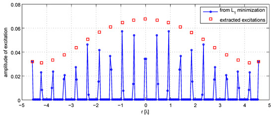
Figure 1.
Excitations found by minimization.
It is evident that the “right” position of excitations has to be taken in an average coordinate between the two points. Let now and be the position of two adjacent samples, of excitation and ; the chosen position and excitation of the sparse element are then provided by
By means of this “clustering”, the overall number of excitations is reduced to 21 (that is the same value obtained by means of a much more cumbersome hybrid algorithm); the clustering in this case has a marginal effect on the the radiated pattern, which does not satisfy the power pattern mask for a fraction of dB; we can then perform a quick optimization of the excitations (always by means of CVX) in order to find the final pattern, which is provided in Figure 2.
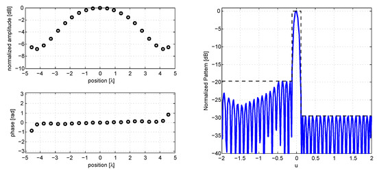
Figure 2.
The achieved 21 element asymmetric pencil beam layout. On the left: normalized amplitude and excitation phase; on the right: pencil beam pattern with its upper mask.
It is of paramount importance to emphasize two main differences with respect to [12]: first, we use a dense equispaced excitation vector that is sampled in a much coarser way () instead of ), with a significant computational advantage; second, by means of the excitations’ clustering, we are able to perform, in most practical cases, a single minimization, instead of multiple sequential ones, to achieve the desired result. Because of these two differences, the whole computation of the pencil beam pattern, including the final local optimization of the excitations, requires less than 20 s on an office PC running Matlab and CVX with an i5-2310 processor (Intel Corporation, Santa Clara, CA, USA).
We must underline that the simple minimization is not always capable of providing a sparse solution, particularly if we deal with the synthesis of a pencil beam with a symmetrical level of the sidelobes. To overcome this problem it is possible to use the technique of sequential convex optimizations, similarly to [12]: in the first step, we solve the problem defined by Equations (6) and (7), and in the successive ones, the non-sparse solution obtained in step is employed to build a weighted norm problem as:
where and ϵ is a small constant, of the order of the minimum excitation we want to obtain.
As an example, we can consider the synthesis of a sparse pencil beam array ( dB for and ); by means of Bayesian compressive sensing [11], the specification can be met with 24 elements, and almost met with 20 elements; by means of an evolutionary algorithm [22], it was possible to use 19 radiating elements. With just 15 iterations of the minimization Equations (11)–(13), we are able to achieve a layout employing the same number of elements of the evolutionary approach in Figure 3, and the specifications are perfectly met.
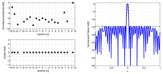
Figure 3.
The achieved 19 element symmetric pencil beam layout. On the left: normalized amplitude and excitation phase; on the right: pencil beam pattern with its upper mask.
3. The SFGAP Algorithm
The convex nature of the pencil beam synthesis allowed us to obtain a quick and efficient solution by means of a simple minimization. In general cases, the sparse array pattern synthesis is formulated in terms of an upper and a lower power pattern mask (Figure 4), as:
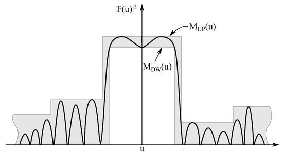
Figure 4.
Power pattern mask.
Unfortunately, the above formulation does not lead to a convex problem, for which we can rapidly employ the computationally efficient methods of software packages like CVX. Other researchers have employed minimization approaches for a shaped beam synthesis problem, like in [12], but, in such approaches, the “shaped part” of the beam, i.e., the part of the beam that is constrained between the upper mask and a non-null lower mask, is usually sought approximating a known or given pattern in amplitude and phase. In the approach that we will discuss in this paper, we just want to define the two power pattern masks without trying to approximate a known function, making the approach more general.
This aim is realized by introducing the SFGAP method.
Let us briefly recall the general principle of the GAP (Generalized Alternate Projections) algorithm [15]. The GAP achieves the excitation of a fixed element position array by alternatively projecting the solution on two sets: the set of the fields that can be radiated from the fixed positions, and the set of the patterns that belong to the specification’s power pattern mask.
The SFGAP algorithm differs from a standard GAP for two main reasons: first of all, the sources’ positions are taken closely spaced (much less than half the free-space wavelength) within the range in which we want to synthesize the sparse array; second, the projection on the subspace of the field that can be radiated by those closely spaced radiators is constrained by the solution of a convex problem that is similar to the norm minimization that has been employed for the pencil beam case.
Let us now discuss the two projections to be used in SFGAP; according to the notation introduced in the previous paragraph, the projected field on the mask defined by Equations (14) and (15) can be realized by means of the well-known rule [1]:
The projection of the field on the space of the fields that can be radiated by the closely spaced sources can be achieved by a compressive sensing like approach, solving the problem:
where τ is a proper threshold, the value of which will be discussed in the next paragraph.
While the projection on the set of fields belonging to the power pattern mask does not require any discussion, besides the fact that the set of fields may not be convex because of the presence of the lower mask, the latter projection needs some discussion.
The solutions of Equations (20) and (21) lead to the set of excitations whose norm is below the threshold τ that is as close as possible to the field ; the set defined by Equation (21) is a convex set, and because of the linearity of the relationship (5), also the set of fields , in which we are considering the minimization (20), is convex. Furthermore, it is easy to demonstrate that for .
We also need to underline that, differently from the minimization used in Equations (6) and (7), in this case, we minimize the distance of two fields with a threshold on the maximum norm of the excitation, but, as it will be shown in the following, it leads to a sparse solution as well.
By alternating the projections on the two sets, and , we should be able to find a solution belonging to the two sets, but there are two aspects that we should take into account. First, as stated before, the set can be non-convex: when dealing with the GAP, in these cases, we usually need to pay particular attention to the choice of the starting point of the algorithm. Otherwise, it can be trapped in a local minimum, thus preventing the convergence to a solution belonging to the intersection of the two sets (see Figure 5a).
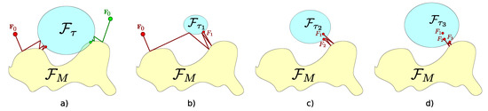
Figure 5.
Scheme of the alternate projections. (a) the choice of a wrong starting point (red) can lead to local minima; the choice of a good starting point (green) can lead to a solution; (b) if τ is too small, there could be no intersection of sets; and (c,d) smoothly increasing the value of τ allows for moving towards the solution of the starting problem.
Secondly, for a particular choice of τ, we can not be sure that an intersection of the two sets exists, so we should choose a reasonable value of τ for the SFGAP to work correctly (see Figure 5b).
A possible strategy, which in our numerical experiments proved to be very robust, consists of starting the projections with a very low value of τ; when the algorithm reaches a “trap”, the value of the threshold is increased and the projections start again. In Figure 5c,d we provide a graphical representation of this behaviour, showing the effect of an increasing value of τ.
The choice of starting with a low value of the threshold, and then slowly increasing it can surely solve the problem of choosing the correct value of τ, but it also makes the algorithm less sensitive to the choice of a bad starting point. With reference to Figure 5b–d, let us consider the sequence of fields , and represented as “points” in which the algorithm has “stopped” when the threshold was, respectively, , and , with . If the intersection of and exists, such a sequence points in the direction of the intersection, so even if we choose a bad starting point (as in Figure 5a), we would be able to find the solution of the synthesis problem that we are dealing with: we will find the field that fits into the power pattern mask, with the minimum norm for the excitation.
Obviously, we can not completely avoid the problem of a bad starting point (nor the presence of multiple solutions), but in our numerical trials, we have found that within a few trials of the random starting field, we can reach the sought after solution.
What we need to achieve this desired behaviour is just a proper “increasing” strategy for the threshold. We can not increase it too slowly; otherwise, the synthesis would take too much time. Accordingly, we can not increase it too quickly. Otherwise, we could not find the field with minimum norm for the excitation.
After some numerical testing, we found that a robust yet efficient strategy for obtaining a good value for the threshold can be achieved by evaluating, at each iteration p, the quantity:
where is the field belonging to at iteration p, is the field belonging to at iteration p, and is the value of the threshold employed in iteration p, updated according to:
where pc is a small integer, and α and γ are two constants.
The main idea is to check when the relative decrease of within iterations is lower than α. If this is true, a local minimum of the algorithm is detected, and the value of is increased with a factor that depends on the actual distance of the fields , by means of the multiplicative constant γ.
In our trials, we have found that values of , , and usually lead to a good compromise of speed and accuracy of the overall algorithm. Such values have been used for all of the examples that we provide in the next section.
In summary, the SFGAP algorithm consists of the following steps:
- Set the iteration counter , and define a random starting pattern and a value of ;
- Increase the iteration counter p and evaluate the projection of the pattern on by Equations (17)–(19);
- Calculate the field as the projection of on by Equations (20) and (21);
- Evaluate by means of Equation (22), and if , calculate the value of (to be used in the next iteration) according to Equations (23) and (24);
- If the termination conditions are met (for instance, a maximum value of iterations and/or a minimum value of is achieved), the algorithm stops; otherwise, go back to step 2.
The starting value of can have a small influence on the quickness of the convergence of the algorithm, since if its value is close to the final value, the overall number of iterations needed to find the solution can be lower, but such a number can be hard to guess, so, in our numerical tests, we have always used as the starting value, leaving to the adaptive increasing rules (23) and (24) the duty of finding the correct value for τ.
It is worth noting that the SFGAP shares some similarities with the CSGAP proposed in [14]; both of the algorithms are an extension of the generalized alternate projection algorithm, but in the CSGAP at each iteration, we solve the following minimization problem:
where is the threshold at step h, which is chosen according to the following rule , being the starting value of the threshold. The use of Equations (25) and (26) is very sensitive with respect to the choice of the starting point and of , making this algorithm much less “stable” and effective with respect to the SFGAP introduced in the present paper. In the following, we will provide some examples of applications of the proposed method.
4. Results
To validate the proposed approach, we will now show the results of some synthesis examples; in particular, we will discuss two sparse arrays, capable of radiating a flat-top beam to be employed—for instance, in a virtual subarray radar architecture [23].
As the first test case, we will investigate a flat-top synthesized by other researchers [12,24,25] who have tried to minimize the number of feeds required to achieve the pattern with the desired specifications ( for , for ), finding that a minimum number of 10 elements is needed.
By means of the SFGAP we are also able to find a sparse array with 10 elements, radiating a pattern satisfying the mask constraints (see Figure 6, providing excitations, overall pattern and a particular of the flat top region), but without seeking a preliminarily calculated solution, as in the methods employed by other researchers.
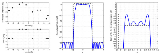
Figure 6.
The first flat-top pattern achieved by means of SFGAP; from left to right: amplitude and phase of the excitations, power pattern of the array with its mask, highlight of the flat-top part of the pattern.
In a second example, we consider the flat-top pattern specifications used in [26], in particular, the case with 31 radiating elements ( for , for ). In our case, the SFGAP is capable of satisfying the same power pattern mask with only 19 radiating elements (see Figure 7, providing excitations, overall pattern and a particular of the flat top region).
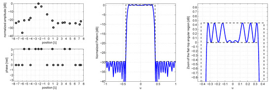
Figure 7.
The second flat-top pattern achieved by means of SFGAP; from left to right: amplitude and phase of the excitations, power pattern of the array with its mask, highlight of the flat-top part of the pattern.
In a third example, we would also like to consider in the synthesis the presence of an element factor; following the specifications used in [26], in particular, the case with 19 radiating elements ( for , for ), with an element factor that multiplies the array factor in Equation (4). This requires us to multiply all of the columns of matrix for the sampled vector of the element factor, but this has no other effects on the overall synthesis approach.
The results of the synthesis are provided in Figure 8 (in which we plot the excitations, the overall pattern and a particular of the flat top region), where we can see that the specifications can be met with 12 elements only, and the ripple is much lower with respect to the specifications (about 0.5 dB instead of 1 dB).
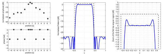
Figure 8.
The third flat-top pattern achieved by means of SFGAP; from left to right: amplitude and phase of the excitations, power pattern of the array with its mask, highlight of the flat-top part of the pattern.
5. Discussion
The results provided in the previous paragraph confirm the good performances of the SFGAP. In particular, we were capable of matching the results provided by other methods that require the preliminary synthesis of a pattern to be sought, and, in other cases, we achieve the satisfaction of the constraints with a much lower number of radiating elements.
In the paper, we have not considered the effect of the mutual coupling among elements; this is a reasonable assumption for sparse arrays, for which the element spacing is usually greater than a half-wavelength, and the main effect of mutual coupling consists in modifying the actual excitation on radiating elements with respect to the imposed voltages on the generators; in this case, once the position of the elements is achieved, it is trivial to calculate the proper compensation of the excitations [27].
Furthermore, besides the asymmetric pencil beam case (where the power pattern mask was defined in the range to allow the scanning of the beam in the whole visible range without the appearance of the grating lobes), we have not considered the effect of the scanning of the beam; this could be achieved by simply increasing the range of u in which we want the satisfaction of the power pattern mask. Furthermore, in such a case, we could also take into account the presence of an element factor (that could change the side lobe level when the beam is scanned) by considering a modified power pattern mask, following the guidelines proposed in [28].
It also has to be underlined that we may need to try some different random starting patterns , but, in most cases, few trials are sufficient to find a good final result. It is also interesting to observe that different starting points could lead to slightly varied, but equally acceptable, solutions. Generally speaking, these solutions show the same number of radiating elements but a different element spacing or excitation dynamic, so we could exploit this feature of the algorithm in order to have a set of different layouts from which we could choose the one to implement.
Finally, the number of iterations needed to achieve all of the results shown is lower than 100, and the single iteration for these example takes 10 to 20 seconds on an office PC, running Matlab and CVX, with a i5-2310 processor (a low-end processor with respect to current CPUs), Thus, the single synthesis usually takes less than half an hour.
6. Conclusions
In this paper, we have introduced an SFGAP algorithm for the synthesis of sparse array patterns.
The main characteristic of the proposed algorithm with respect to others available in the open literature is the fact that SFGAP does not try to find a sparse array emulating the radiation of a desired pattern, but still allows a deterministic solution of the sparse array synthesis problem. The fact that we can rely on a deterministic approach instead of using a “brute force” evolutionary optimization method is of paramount importance from a computational point of view.
The algorithm is simple and flexible, since it is based on power pattern masks. It is also possible, with minor modifications, to deal with conformal arrays [29]. The numerical examples provided in the contribution show good synthesis results.
For future developments, we are working towards the application of the presented technique also for planar arrays, in particular to sparse circular arrays [30,31] and to plane wave generators [32,33]. We are also looking for the introduction of additional system constraints in the synthesis method, like a minimum or maximum inter-element distance, or a particular dynamic of the excitations.
Author Contributions
D.P., M.D.M. and G.P. conceived the SFGAP method; D.P. wrote the numerical code and performed the array syntheses; M.D.M., M.L. and F.S. helped with the comparison with other approaches; D.P., G.P. and F.S. wrote the paper.
Conflicts of Interest
The authors declare no conflict of interest.
References
- Bucci, O.; Franceschetti, G.; Mazzarella, G.; Panariello, G. Intersection approach to array pattern synthesis. IEE Proc. H-Microw. Antennas Propag. 1990, 137, 349–357. [Google Scholar] [CrossRef]
- Lebret, H.; Boyd, S. Antenna array pattern synthesis via convex optimization. IEEE Trans. Signal Process. 1997, 45, 526–532. [Google Scholar] [CrossRef]
- Nemirovski, A.; Yudin, D.B.; Dawson, E.R. Problem Complexity and Method Efficiency in Optimization; John Wiley & Sons Ltd: Hoboken, NJ, USA, 1982. [Google Scholar]
- Skolnik, M. Nonuniform Arrays. In Antenna Theory, Part I; McGraw-Hill: New York, NY, USA, 1969; Chapter 6; Volume 42. [Google Scholar]
- Mazzarella, G.; Panariello, G. A projection-based synthesis of non-uniform array. In Proceedings of the Antennas and Propagation Society International Symposium, London, ON, Canada, 24–28 June 1991; pp. 1164–1167.
- Bucci, O.M.; Perna, S.; Pinchera, D. Advances in the deterministic synthesis of uniform amplitude pencil beam concentric ring arrays. IEEE Trans. Antennas Propag. 2012, 60, 3504–3509. [Google Scholar] [CrossRef]
- Migliore, M.D.; Pinchera, D. Compressed sensing in electromagnetics: Theory, applications and perspectives. In Proceedings of the 5th European Conference on Antennas and Propagation (EUCAP), Rome, Italy, 11–15 April 2011.
- Migliore, M.D. A simple introduction to compressed sensing/sparse recovery with applications in antenna measurements. IEEE Antennas Propag. Mag. 2014, 2, 14–26. [Google Scholar] [CrossRef]
- Costanzo, S.; Borgia, A.; Di Massa, G.; Pinchera, D.; Migliore, M.D. Radar array diagnosis from undersampled data using a compressed sensing/sparse recovery technique. J. Electr. Comput. Eng. 2013, 2013, 8. [Google Scholar] [CrossRef]
- Migliore, M.D. On the sampling of the electromagnetic field radiated by sparse sources. IEEE Trans. Antennas Propag. 2015, 63, 553–564. [Google Scholar] [CrossRef]
- Oliveri, G.; Carlin, M.; Massa, A. Complex-weight sparse linear array synthesis by Bayesian compressive sampling. IEEE Trans. Antennas Propag. 2012, 60, 2309–2326. [Google Scholar] [CrossRef]
- Fuchs, B. Synthesis of sparse arrays with focused or shaped beampattern via sequential convex optimizations. IEEE Trans. Antennas Propag. 2012, 60, 3499–3503. [Google Scholar] [CrossRef]
- Morabito, A.F.; Laganà, A.R.; Isernia, T. Improving performances of Compressive Sensing in the synthesis of maximally-sparse arrays. In Proceedings of the 2014 IEEE Antennas and Propagation Society International Symposium (APSURSI), Memphis, TN, USA, 6–11 July 2014; pp. 61–62.
- Pinchera, D.; Migliore, M.D. Effective sparse array synthesis using a generalized alternate projection algorithm. In Proceedings of the IEEE Conference on Antenna Measurements & Applications (CAMA), Antibes Juan-les-Pins, France, 16–19 November 2014; pp. 1–2.
- Bucci, O.M.; D’Elia, G.; Mazzarella, G.; Panariello, G. Antenna pattern synthesis: A new general approach. Proc. IEEE 1994, 82, 358–371. [Google Scholar] [CrossRef]
- Deng, W.; Yin, W.; Zhang, Y. Group sparse optimization by alternating direction method. In SPIE Optical Engineering + Applications; International Society for Optics and Photonics: Bellingham, WA, USA, 2013; p. 88580R. [Google Scholar]
- Li, K.; Sundin, M.; Rojas, C.R.; Chatterjee, S.; Jansson, M. Alternating strategies with internal ADMM for low-rank matrix reconstruction. Signal Process. 2016, 121, 153–159. [Google Scholar] [CrossRef]
- Baraniuk, R.G. Compressive sensing. IEEE Signal Process. Mag. 2007, 24, 1–9. [Google Scholar] [CrossRef]
- Grant, M.; Boyd, S. CVX: Matlab Software for Disciplined Convex Programming, Version 2.1. Available online: http://cvxr.com/cvx (accessed on 20 December 2016).
- Isernia, T.; Ares, F.; Bucci, O.M.; D’Urso, M.; Gómez, J.F.; Rodriguez, J. A hybrid approach for the optimal synthesis of pencil beams through array antennas. In Proceedings of the IEEE Antennas and Propagation Society International Symposium, Monterey, CA, USA, 20–25 June 2004; Volume 3, pp. 2301–2304.
- Mailloux, R.J. Phased Array Antenna Handbook; Artech House Boston: Norwood, MA, USA, 2005; Volume 2. [Google Scholar]
- Cen, L.; Ser, W.; Yu, Z.L.; Rahardja, S.; Cen, W. Linear sparse array synthesis with minimum number of sensors. IEEE Trans. Antennas Propag. 2010, 58, 720–726. [Google Scholar]
- Pinchera, D.; Migliore, M.D.; Panariello, G. A Virtual Subarray Architecture for Imaging Radar. IEEE Trans. Antennas Propag. 2014, 62, 5171–5179. [Google Scholar] [CrossRef]
- Liu, Y.; Liu, Q.H.; Nie, Z. Reducing the number of elements in the synthesis of shaped-beam patterns by the forward-backward matrix pencil method. IEEE Trans. Antennas Propag. 2010, 58, 604–608. [Google Scholar]
- Pinchera, D.; Migliore, M.D. Comparison guidelines and benchmark procedure for sparse array synthesis. Prog. Electromagn. Res. M 2016, 52, 129–139. [Google Scholar]
- Nai, S.E.; Ser, W.; Yu, Z.L.; Chen, H. Beampattern synthesis for linear and planar arrays with antenna selection by convex optimization. IEEE Trans. Antennas Propag. 2010, 58, 3923–3930. [Google Scholar] [CrossRef]
- Hui, H.T. Decoupling methods for the mutual coupling effect in antenna arrays: A review. Recent Pat. Eng. 2007, 1, 187–193. [Google Scholar]
- Bucci, O.M.; Isernia, T.; Perna, S.; Pinchera, D. Isophoric sparse arrays ensuring global coverage in satellite communications. IEEE Trans. Antennas Propag. 2014, 62, 1607–1618. [Google Scholar] [CrossRef]
- Mazzarella, G.; Panariello, G. Pattern synthesis of conformal arrays. In Proceedings of the Antennas and Propagation Society International Symposium, Ann Arbor, MI, USA; 1993; pp. 1054–1057. [Google Scholar]
- Bucci, O.M.; Pinchera, D. A generalized hybrid approach for the synthesis of uniform amplitude pencil beam ring-arrays. IEEE Trans. Antennas Propag. 2012, 60, 174–183. [Google Scholar] [CrossRef]
- Bucci, O.M.; Perna, S.; Pinchera, D. Synthesis of isophoric sparse arrays allowing zoomable beams and arbitrary coverage in satellite communications. IEEE Trans. Antennas Propag. 2015, 63, 1445–1457. [Google Scholar] [CrossRef]
- Bucci, O.M.; Migliore, M.D.; Panariello, G.; Pinchera, D. An effective algorithm for the synthesis of a plane wave generator for linear array testing. In Proceedings of the IEEE APS International Symposium, Chicago, IL, USA, 8–14 July 2012; pp. 1–2.
- Bucci, O.M.; Migliore, M.D.; Panariello, G.; Pinchera, D. Plane-wave generators: Design guidelines, achievable performances and effective synthesis. IEEE Trans. Antennas Propag. 2013, 61, 2005–2018. [Google Scholar] [CrossRef]
© 2016 by the authors. Licensee MDPI, Basel, Switzerland. This article is an open access article distributed under the terms and conditions of the Creative Commons Attribution (CC BY) license ( http://creativecommons.org/licenses/by/4.0/).