Few-Shot Cross-Domain Deepfake Detection for Edge Devices: A Feature Decoupled System Architecture

Abstract

Deploying highly generalizable deepfake detection systems on resource-constrained edge devices poses a significant technical challenge for conventional end-to-end large models that rely heavily on computational resources. Extracting multi-source physical prior features is a viable approach under limited computational power; however, in few-shot scenarios, the dimensional mismatch of heterogeneous features is prone to causing downstream classifiers to overfit. To mitigate this bottleneck, this paper proposes a “static feature extraction–central normalization alignment–independent downstream decision” decoupled detection system for few-shot cross-domain tasks on edge devices. The front end of the system constructs an 856-dimensional comprehensive feature reservoir, and a lightweight residual normalization adapter $g_{\varphi }$ is introduced as the central support module. This module explicitly compresses the intra-class variance of heterogeneous features, providing a smoothly aligned manifold base for downstream classifiers. Experimental results indicate that this decoupled architecture demonstrates consistent stability in few-shot ($K=10$) cross-domain evaluations. When encountering intra-family cross-domain shifts and cross-mechanism distribution shifts from diffusion models, the accuracy reaches 84.9% and 76.1%, respectively. Compared to representative end-to-end meta-learning baselines (e.g., MAML), the relative error rate is reduced by over 30%. Furthermore, after completing the asynchronous offline pre-processing (approximately 897 ms) at the front end, a single-image online classification query requires only 7.7 ms under a simulated single-core CPU constraint, satisfying the low-latency requirements for lightweight deployment on edge devices. Finally, combined with empirical observations, this paper discusses the performance boundaries of the architecture in cross-mechanism metric mismatch scenarios, providing a low-barrier, robust engineering defense scheme for resource-constrained environments.

1. Introduction

In an open-world environment, few-shot cross-domain classification aims to adapt a model to an unseen target domain using only a handful of annotated samples. In practice—particularly in digital forensics and industrial inspection—this task faces three simultaneous constraints: the target may come from an unseen distribution (domain shift), annotated samples are extremely limited ($K\le 10$), and edge devices lack GPU support [1,2]. Under such constraints, computationally intensive end-to-end models are difficult to deploy. Methods based on manually designed physical prior features (e.g., frequency-domain statistics, spatial-domain textures, physiological indicators) offer a lightweight alternative. However, directly concatenating multi-source heterogeneous features into a classifier introduces subspace dimensional mismatch: ensemble tree models struggle to find optimal split points when samples are scarce, leading to performance degradation. Achieving stable classification under the combined conditions of cross-domain shifts, few-shot settings, and limited computational resources remains an open systems engineering problem.

Existing research methods can be broadly categorized into three types. First, methods based on deep features (e.g., ResNet [3], CLIP [2]) perform well on identically distributed data but often face limited performance under significant domain shifts. Second, meta-learning methods (e.g., ProtoNet [4], MAML [5]) enhance model adaptability through task-level training. However, these methods typically involve a tightly coupled end-to-end process between feature extraction optimization and classification decisions [6]. When the physical characteristics of target domain data deviate from the model’s training distribution, the failure of the classification head can lead to a weakening of the overall discriminative ability of the system. Finally, methods based on heterogeneous physical prior features have lower computational overhead, but their systematic architectural optimization under few-shot cross-domain protocols requires further investigation.

Overall, a key limitation of existing architectures for few-shot tasks on edge devices is that feature-space alignment and downstream decision boundaries are tightly coupled. Under extreme computational constraints and significant distribution shifts, this coupling makes the metric space fragile. Physically decoupling the feature manifold alignment from task-specific classification decisions therefore emerges as an engineering-feasible solution.

Based on this observation, this paper proposes a few-shot cross-domain decoupled detection system designed for edge deployment. The system separates the operational pipeline into three stages: the front end uses a static, parameter-free pipeline to extract multi-dimensional physical priors; the center introduces a plug-and-play lightweight residual normalization adapter $g_{\varphi }$ to compress intra-class variance and mitigate dimensional mismatch; the back end trains a lightweight classifier (e.g., RF, SVM, or XGBoost) independently on the aligned features for target-domain adaptation.

The main contributions of this paper are summarized as follows:

1.

We propose a “feature extraction–normalization alignment–independent decision” decoupled detection framework for few-shot tasks on edge devices. Compared to tightly coupled end-to-end models, this system effectively reduces the risk of feature space collapse under significant distribution shifts through architectural modular separation, providing a lightweight and robust system pipeline for detection tasks constrained by pure CPU computing power.

2.

We introduce a lightweight residual normalization adapter $g_{\varphi }$ as the central alignment module. Experiments confirm that this adapter provides a variance-aligned smooth manifold base, yielding measurable improvements for ensemble tree models under extremely limited samples ($K=1,3$) and effectively reducing the relative error rate in cross-domain evaluations.

3.

Based on qualitative signal analysis and statistical observations, we discuss the applicable boundaries of the framework. Combining spectral orthogonality and ablation experiments, we analyze the mechanism of “normalization-dominated, residual-assisted” alignment, and explore the performance limitations of linear alignment architectures when facing cross-mechanism generative models (e.g., from GAN to diffusion models), providing a reference for the system’s deployment evaluation in practical engineering.

2. Related Work

2.1. Few-Shot and Cross-Domain Classification

Few-shot classification aims to use a very small number of annotated samples to achieve rapid recognition of new categories by the model. Traditional meta-learning pipelines (such as ProtoNet [4] and MAML [5]) learn a general initialization or metric space through continuous training on multi-task datasets. However, when there are significant physical differences between the target domain and the source domain, these methods often face performance fluctuations under end-to-end coupling [7,8].

2.2. Feature Optimization and Decoupled Adaptation Architectures

In complex cross-domain tasks, decoupling the optimization of feature representation from the classification decision process has become an effective way to improve system robustness [6]. Standard end-to-end learning methods tend to force the feature extractor to adapt to a specific classification head, which is prone to triggering decision boundary failures when facing significant domain shifts. Some studies have introduced lightweight adapters [9] for parameter-efficient fine-tuning; however, these adapters are typically inserted within a deep backbone and still require end-to-end gradient flow during inference. This paper differs in a fundamental architectural aspect: rather than adapting internal representations of a single network, we physically separate the feature normalization operation from the shallow decision process at the system level. The front-end feature extractor is entirely static (no learnable parameters at inference time), the central $g_{\varphi }$ adapter is pre-trained offline and frozen, and the back-end classifier is trained independently on the aligned features. This three-stage physical decoupling eliminates the gradient coupling between feature extraction and classification that causes metric-space fragility in existing adapter-based methods, and enables each module to be independently replaced or upgraded without retraining the others.

2.3. Application Examples of Physical Prior Features

Physical prior features have application value in tasks requiring high interpretability and low computational overhead. Taking deepfake detection as an example, periodic fingerprints left by Generative Adversarial Networks in the image frequency domain [10,11] and high-frequency anomalies in diffusion models [8] are key clues. Recent surveys [12,13] have systematically catalogued these detection cues and benchmarked existing methods. However, there is high heterogeneity and dimensional mismatch among these low-level features (such as LBP [11], GLCM [14]). How to utilize them to build robust classification surfaces under few-shot constraints is an engineering challenge.

2.4. Gradient Boosting and Modern Ensemble Classifiers

Gradient boosting trees represent the mainstream paradigm for tabular data classification. Algorithms like XGBoost [15], LightGBM [16], and CatBoost [17] perform excellently when ample training data is available. However, in extremely few-shot ($K\le 10$) scenarios, split point searches are prone to degradation due to insufficient statistical bases. By using a central adapter to pre-align feature dimensions, this system aims to provide a “statistically friendly” underlying input for these classifiers, encouraging ensemble models to maintain reasonable discriminative capabilities in edge scenarios.

3. Methodology

3.1. Problem Formulation and Feature Representation

Assume there are several source domains $D_{source}$, and the target domain $D_{target}$ is an unseen distribution during the training phase. Given the target domain support set $S={\left\{({\mathbf{x}}_i,y_i)\right\}}_{i=1}^{2K}$, where $y_i\in \{0,1\}$ and each class has only K samples, the goal is to construct a discriminant function $h\left(\mathbf{x}\right)$ for binary classification. Furthermore, the inference pipeline must satisfy the constraints of edge devices, which operate without large-scale annotations and under low computational power.

To achieve reliable detection under the aforementioned conditions, this system avoids the heavy feature extraction of end-to-end large models and employs a static pipeline to construct an 856-dimensional comprehensive feature reservoir ${\mathbf{f}}_0\left(\mathbf{x}\right)$. This feature pool is designed to preserve the complete original data distribution for the subsequent normalization module. The specific extraction logic is as follows:

• Original Physical Features (144 dimensions): Lightweight image signal processing executed on the CPU:

  -

  Frequency-domain illumination (48 dims): Convert images to the HSV color space, extracting 12 statistical indicators (e.g., mean, variance) on the V channel across 4 sub-regions [10,18,19].

  -

  Spatial-domain texture (84 dims): Extract LBP and GLCM statistics in corresponding sub-regions to capture high-frequency discontinuities [11].

  -

  Ocular physiology (12 dims): Extract clarity, symmetry, and fine-grained pupil metrics from the left and right eye regions.

• Original Deep Semantic Features (256 dimensions): This utilizes a pre-trained ResNet-18 with the classification layer removed. ResNet-18 is specifically selected as the semantic backbone because its relatively small parameter footprint and low computational complexity inherently align with the strict resource constraints of edge devices, while still providing sufficient deep feature distinctiveness. Activation vectors are extracted for both face crops and full images, yielding 256-dimensional descriptors via truncated concatenation (accelerated by ONNX Runtime).
• Hybrid Aligned Features (456 dimensions): To mitigate the initial mismatch between physical and deep features, the system zero-pads and truncates the aforementioned physical features into a 200-dimensional space, concatenating them with the 256-dimensional deep features to form a comprehensive feature representation. The 200-dimensional padding is chosen as the smallest power-of-fifty ceiling that accommodates all 144 physical feature dimensions with headroom for future feature additions, while keeping the padded physical block and the 256-dimensional deep block at comparable scales to prevent one modality from dominating during downstream processing.

Ultimately, the system concatenates the above features to output an 856-dimensional vector ($144+256+456$). The deliberate retention of all three feature groups—raw physical, raw deep, and the pre-aligned hybrid—is not merely to increase dimensionality, but to provide the central $g_{\varphi }$ module with maximally diverse input signals for alignment and variance compression. Retaining the raw sub-vectors alongside the hybrid concatenation allows $g_{\varphi }$ to exploit both the original fine-grained distributions and the coarsely aligned representation simultaneously. Concurrently, the ensemble tree models (e.g., Random Forest) selected for the backend inherently possess feature selection and anti-overfitting properties for high-dimensional sparse features, thereby mitigating the risk of the curse of dimensionality at the architectural level when $K\le 10$.

3.2. Lightweight Residual Normalization Adapter $g_{\varphi }$

To address the dimensional mismatch of the feature pool, the system introduces a lightweight residual normalization adapter $g_{\varphi }$:

$${\mathbf{x}}^{\prime }=g_{\varphi }\left(\mathbf{x}\right)=\mathrm{LN}\left(\mathbf{x}+\alpha ·W\mathbf{x}\right)$$

(1)

where $\varphi =\{W,\alpha ,\gamma ,\beta \}$ represent the learnable parameters: $W\in {\mathbb{R}}^{d\times d}$ is the linear projection matrix, $\alpha \in \mathbb{R}$ is the residual coefficient, and $\gamma ,\beta \in {\mathbb{R}}^d$ are the affine parameters inside LayerNorm. LayerNorm performs adaptive bias correction and dimension-wise scaling, aiming to smooth the dimensional disparities among heterogeneous features. The residual term $\alpha ·W\mathbf{x}$ is introduced to ensure that the normalization process does not overly disrupt the spatial topology of the original physical priors.

3.2.1. Optimization Engine Driving Mechanism

As a plug-and-play module, $g_{\varphi }$ needs to learn a cross-domain general normalization mapping. This paper uses classic meta-learning algorithms as the “optimization engine” to drive its parameter updates, rather than proposing a new meta-learning theory:

Metric-based Prototypical Optimization. Compute the class prototypes transformed by $g_{\varphi }$:

$${\mathbf{c}}_k={\displaystyle \frac{1}{K}}\sum _{({\mathbf{x}}_i,y_i)\in \mathcal{S},y_i=k}{g}_{\varphi }\left({\mathbf{f}}_0\left({\mathbf{x}}_i\right)\right),k\in \{0,1\}$$

(2)

The training loss is the average cross-entropy over cross-domain episodes:

$$\mathcal{L}\left(\varphi \right)=-{\displaystyle \frac{1}{\left|\mathcal{Q}\right|}}\sum _{(\mathbf{x},y)\in \mathcal{Q}}log{\displaystyle \frac{exp\left(-{∥g_{\varphi }\left({\mathbf{f}}_0\left(\mathbf{x}\right)\right)-{\mathbf{c}}_y∥}_2^2\right)}{{\sum }_{k^{\prime }}exp\left(-{∥g_{\varphi }\left({\mathbf{f}}_0\left(\mathbf{x}\right)\right)-{\mathbf{c}}_{k^{\prime }}∥}_2^2\right)}}$$

(3)

After completing the offline optimization on the source domains, the parameters of $g_{\varphi }$ are frozen and deployed as the system’s static pre-processing component.

3.2.2. Training Protocol and Hyperparameters

The optimization of $g_{\varphi }$ follows an episodic meta-training protocol. In each episode, a 2-way K-shot support set is sampled from the source domains (with the query domain randomly selected from the fake training domains), and a query set of 15 samples per class is drawn from a held-out split of the same domain. The meta-training runs for up to 500 episodes with early stopping (patience = 50 episodes based on validation loss). The optimizer is Adam with a learning rate of ${10}^{-3}$. The residual coefficient $\alpha$ is initialized to 0.1 and treated as a learnable parameter. Meta-validation uses a held-out source domain (StyleGAN2) to monitor convergence. Three random seeds (42, 123, 456) are used across all experiments, and results are reported as mean ± standard deviation. The 80/20 train/test split within each domain is fixed with a split seed of 123 to ensure strict sample-level isolation between meta-training and evaluation.

3.3. Decoupled Learning and Deployment System

During the online deployment phase in the target domain, the decoupled system utilizes the frozen $g_{\varphi }$ as the central adapter. The system exclusively trains shallow classifiers (such as RF, SVM) independently on the optimized features of the $2K$ samples. This design physically decouples the end-to-end binding between feature extraction and decision boundaries, allowing the classification head for specific tasks to focus on extremely few-shot adaptation, reducing the probability of interference from anomalous distributions in unseen domains.

To select the optimal classifier from the candidate pool (RF, SVM, XGBoost), the system employs Leave-One-Out Cross-Validation (LOO-CV) on the support set when $K\ge 5$ (i.e., ≥10 total samples), selecting the classifier with the highest LOO accuracy. For extreme few-shot conditions ($K=1,3$), the support set is too small for reliable cross-validation; in these cases, the system defaults to Random Forest (RF) as the fallback backend. RF is chosen because its ensemble averaging and built-in feature bagging provide strong regularization against overfitting on high-dimensional sparse inputs, making it the most robust single-classifier choice when statistical estimation is unreliable. This fallback strategy strictly isolates query set data and introduces no information leakage.

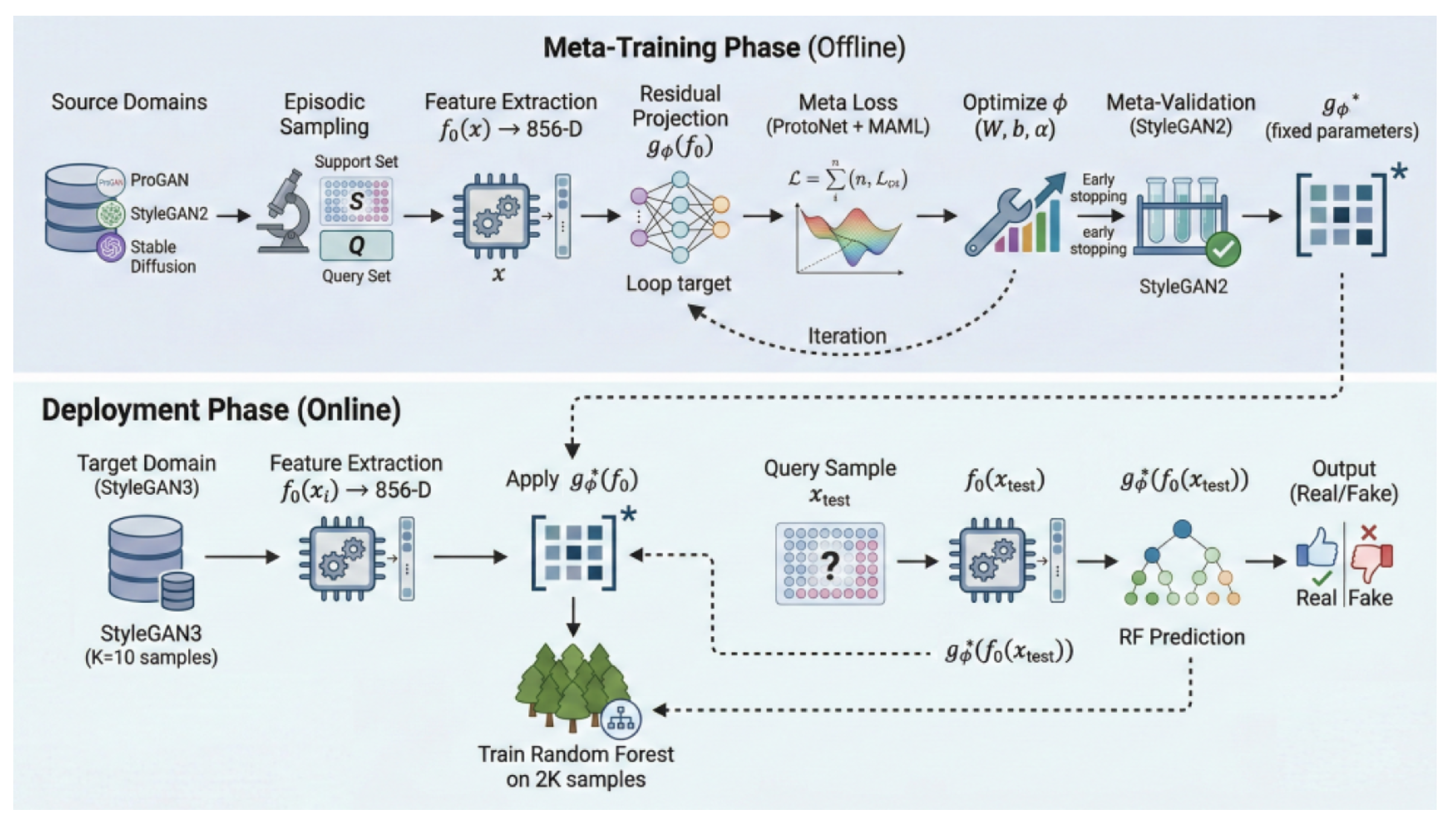
Figure 1 illustrates the complete deployment pipeline, and Algorithm 1 details the corresponding inference procedure, where the entire process can be executed on the CPU side.

Algorithm 1 Inference Pipeline of the Decoupled Adaptation System

Require:  Target domain support set $\mathcal{S}={\left\{({\mathbf{x}}_i,y_i)\right\}}_{i=1}^{2K}$, query sample ${\mathbf{x}}_q$, pre-trained $g_{\varphi }$ (fixed parameters) Ensure:  Predicted label ${\widehat{y}}_q$  1: // Front-end: Static extraction of heterogeneous features (∼897 ms/image, asynchronous offline)  2: for each sample $\mathbf{x}\in \mathcal{S}\cup \left\{{\mathbf{x}}_q\right\}$ do  3:       Detect face and ocular ROI (OpenCV Haar cascade)  4:       Extract illumination features ${\mathbf{f}}_{\mathrm{illum}}\leftarrow {\varphi }_{\mathrm{illum}}\left(\mathbf{x}\right)$          ▹ HSV-V channel, 48 dims  5:       Extract texture features ${\mathbf{f}}_{\mathrm{texture}}\leftarrow {\varphi }_{\mathrm{LBP}}\left(\mathbf{x}\right)\oplus {\varphi }_{\mathrm{GLCM}}\left(\mathbf{x}\right)$          ▹ LBP+GLCM, 84 dims  6:       Extract ocular features ${\mathbf{f}}_{\mathrm{pupil}}\leftarrow {\varphi }_{\mathrm{eye}}\left(\mathbf{x}\right)$             ▹ Eye and pupil stats, 12 dims  7:       Extract deep semantic features ${\mathbf{f}}_{\mathrm{deep}}\leftarrow {\varphi }_{\mathrm{ResNet}}\left(\mathbf{x}\right)$        ▹ ONNX runtime, 256 dims  8:       Basic alignment and concatenation: ${\mathbf{f}}_{\mathrm{comb}}\leftarrow [\mathrm{pad}([{\mathbf{f}}_{\mathrm{illum}};{\mathbf{f}}_{\mathrm{texture}};{\mathbf{f}}_{\mathrm{pupil}}],200);{\mathbf{f}}_{\mathrm{deep}}]$▹ Hybrid, 456 dims  9:       Aggregate the full feature reservoir: ${\mathbf{f}}_0\left(\mathbf{x}\right)\leftarrow [{\mathbf{f}}_{\mathrm{illum}};{\mathbf{f}}_{\mathrm{texture}};{\mathbf{f}}_{\mathrm{pupil}};{\mathbf{f}}_{\mathrm{deep}};{\mathbf{f}}_{\mathrm{comb}}]$  ▹ Total 856 dims 10:      Apply unified z-score standardization 11: end for 12: // Center: $g_{\varphi }$ normalized feature adaptation (∼0.30 ms/image) 13: for each sample $\mathbf{x}\in \mathcal{S}\cup \left\{{\mathbf{x}}_q\right\}$ do 14:      ${\mathbf{x}}^{\prime }\leftarrow g_{\varphi }\left({\mathbf{f}}_0\left(\mathbf{x}\right)\right)=\mathrm{LN}({\mathbf{f}}_0\left(\mathbf{x}\right)+\alpha ·W{\mathbf{f}}_0\left(\mathbf{x}\right))$ 15: end for 16: // Back-end: Target domain independent adaptation & lightweight online query 17: Train the target classifier h (e.g., RF, SVM, XGBoost) on the support set ${\mathcal{S}}^{\prime }$ 18: ${\widehat{y}}_q\leftarrow h\left(g_{\varphi }\left({\mathbf{f}}_0\left({\mathbf{x}}_q\right)\right)\right)$                       ▹ Query latency ≤ 7.7 ms 19: return  ${\widehat{y}}_q$

3.4. Empirical Observations on Generative Mechanism Differences

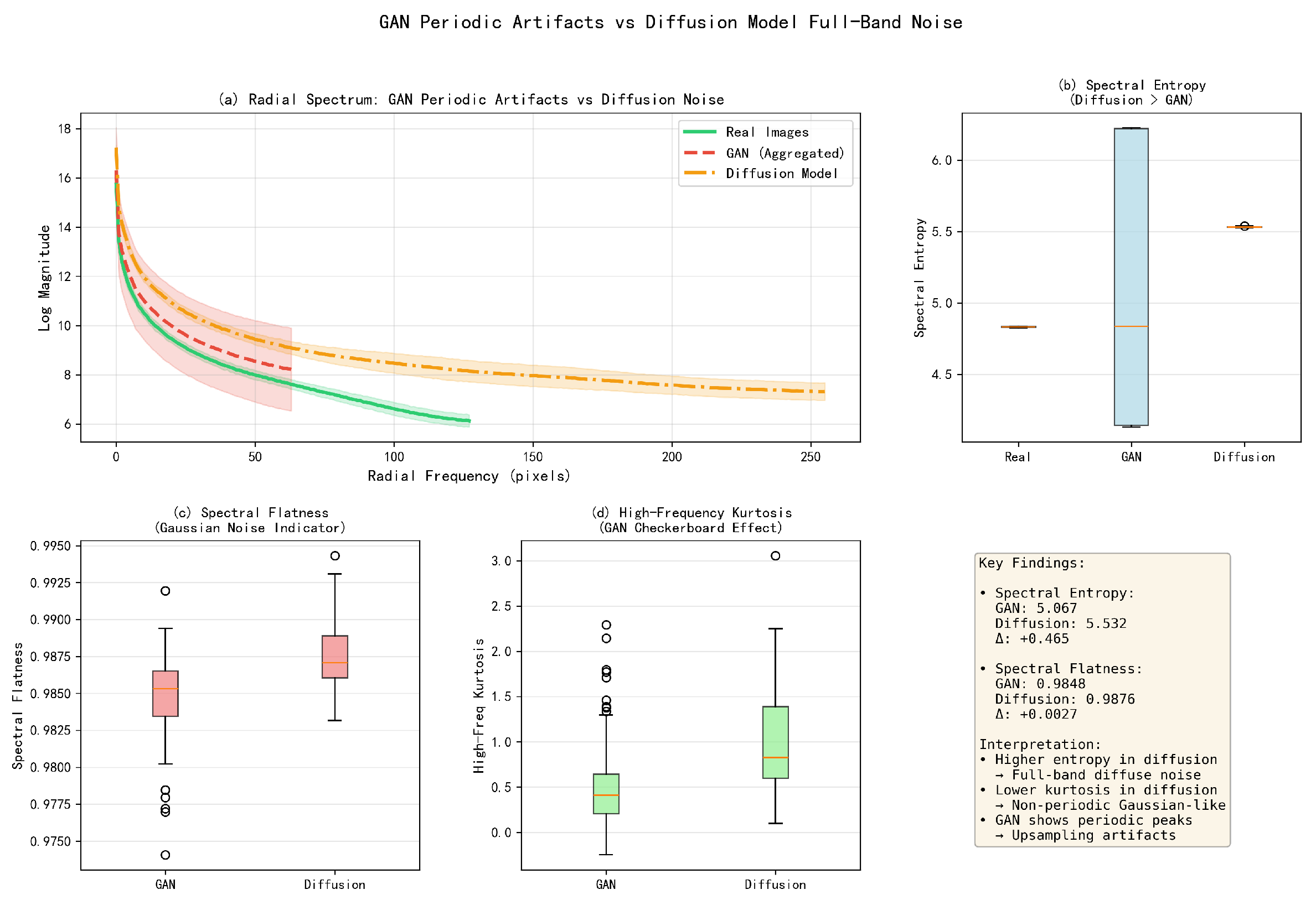
Based on qualitative signal analysis methods, empirical observations of the underlying characteristics of different generative architectures help in understanding the heterogeneous environment faced by the decoupled system. As shown in Figure 2, it is observed that GANs exhibit relatively regular periodic fluctuations in the high-frequency region, whereas diffusion models show a smooth spectral decay, with a flatness closer to diffuse noise.

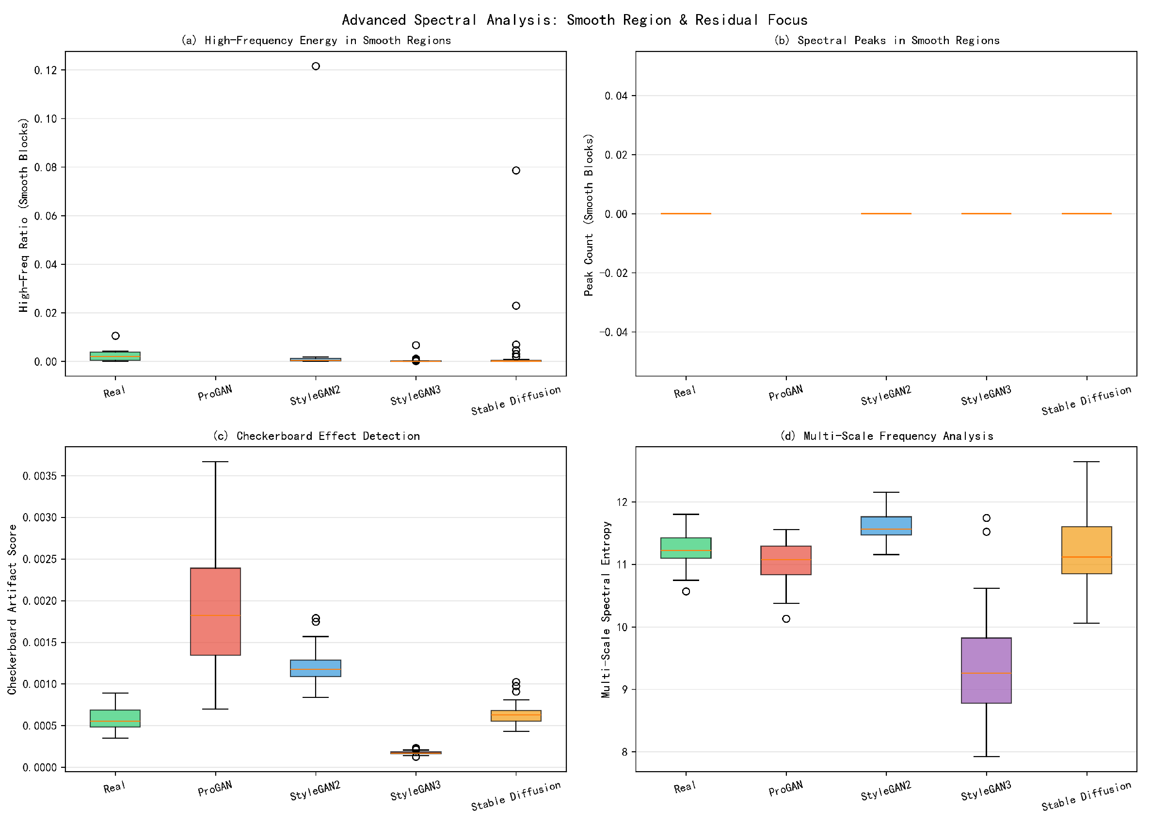
Further fine-grained statistics (Figure 3) show that the checkerboard effect indicators for GANs are generally higher than those for diffusion models. These qualitative signal traits imply that when the system processes intra-family cross-domain tasks within GANs, the feature alignment module is relatively effective because the underlying defects share a similar distribution basis. However, when crossing over to diffusion models with fundamentally different generative mechanisms, the normalization mapping may face challenges.

4. Experimental Evaluation and Application Examples

4.1. Experimental Setup

We constructed binary classification tasks using real faces and generated fake faces (CelebA-HQ, FFHQ, ProGAN, StyleGAN2, StyleGAN3, Stable Diffusion). All images are center-cropped to $224\times 224$ pixels after face detection via OpenCV Haar cascades (with a 20-pixel padding around the detected face bounding box). Eye regions are localized within the detected face for ocular feature extraction. No additional augmentation or compression is applied to the candidate pool. To reduce confounding factors introduced by dataset scale or external compression, we randomly sampled 500 images from each dataset to form a candidate pool for generating few-shot tasks. All candidate pools are class-balanced (250 real, 250 fake per domain pair) and do not differ in compression format or resolution. It should be explicitly noted that these images do not constitute a traditional training set, but serve exclusively as a meta-testing pool. By dynamically sampling numerous independent few-shot episodes from this pool, we ensure that the reported performance reflects a statistically robust expectation of the model’s cross-domain generalization, effectively mitigating the bias of any single small-sample selection. We acknowledge that this curated pool may not fully reflect real-world conditions where data is uncurated, compressed, or drawn from unknown generators. The controlled setting is intentional: it isolates the effect of domain shift from confounding factors (e.g., JPEG artifacts, resolution variation) to enable a fair architectural comparison. Deploying the system in the wild would likely require additional robustness measures such as compression-aware augmentation, which we leave to future work.

Each experimental condition (per K value, per test domain, per seed) is evaluated over 20 independent episodes. Each episode samples K real and K fake images for the support set, and 15 real and 15 fake images for the query set, ensuring strict class balance. Features are z-score standardized per episode (fitted on the support set, applied to both support and query). Across 3 seeds, 2 test domains, and 4 K values, this yields a total of $3\times 2\times 4\times 20=480$ episodes per method.

Two sets of controlled experiments were established: Setting A (SG3-UNSEEN): The source domains include CelebA-HQ (real), FFHQ (real), Stable Diffusion (fake), ProGAN (fake), and StyleGAN2 (fake); the target testing domains are StyleGAN3 (UNSEEN) and ProGAN (SEEN). Although Stable Diffusion is a diffusion-based generator, it is included in the training pool to provide the system with exposure to heterogeneous generative mechanisms during meta-training. The “UNSEEN” designation refers strictly to StyleGAN3, which is withheld entirely from training. Setting B (SD-UNSEEN, Cross-mechanism): The source domains include CelebA-HQ (real), FFHQ (real), ProGAN (fake), StyleGAN2 (fake), and StyleGAN3 (fake); the target testing domain is Stable Diffusion (UNSEEN). This configuration uses exclusively GAN-family generators for training and reserves the diffusion model for testing, enabling a direct evaluation of cross-mechanism generalization. It maintains an equivalent number of fake training domains (three) as Setting A for a controlled comparison.

4.2. System Classifier Matrix Performance Evaluation

To evaluate the universality of this decoupled system as a “feature base,” we tested various independent shallow classifiers on the target domain.

Table 1. Full matrix comparison of cross-domain generalization performance in UNSEEN domains (Accuracy ± std).

		Setting A (SG3-UNSEEN)				Setting B (SD-UNSEEN)
Arch.	Classifier	K = 1	K = 3	K = 5	K = 10	K = 1	K = 3	K = 5	K = 10
Raw	RF (raw)	$0.529\pm 0.042$	$0.794\pm 0.014$	$0.786\pm 0.007$	$0.827\pm 0.008$	$0.590\pm 0.007$	$0.748\pm 0.006$	$0.746\pm 0.007$	$0.746\pm 0.006$
	SVM (raw)	$0.566\pm 0.028$	$0.821\pm 0.020$	$0.847\pm 0.019$	$0.854\pm 0.009$	$0.608\pm 0.009$	$0.708\pm 0.007$	$0.743\pm 0.007$	$0.755\pm 0.006$
	XGBoost	$0.512\pm 0.008$	$0.521\pm 0.011$	$0.668\pm 0.003$	$0.772\pm 0.012$	$0.505\pm 0.004$	$0.513\pm 0.008$	$0.683\pm 0.009$	$0.695\pm 0.007$
	LightGBM	$0.504\pm 0.011$	$0.584\pm 0.031$	$0.692\pm 0.008$	$0.769\pm 0.014$	$0.536\pm 0.007$	$0.640\pm 0.010$	$0.691\pm 0.008$	$0.738\pm 0.009$
	CatBoost	$0.528\pm 0.015$	$0.798\pm 0.010$	$0.791\pm 0.004$	$0.820\pm 0.007$	$0.656\pm 0.009$	$0.738\pm 0.006$	$0.745\pm 0.008$	$0.751\pm 0.006$
	KAN (raw)	$0.637\pm 0.029$	$0.800\pm 0.015$	$0.807\pm 0.029$	$0.829\pm 0.022$	$0.638\pm 0.012$	$0.755\pm 0.006$	$0.771\pm 0.008$	$0.778\pm 0.007$
Ours	RF + $g_{\varphi }$	$0.578\pm 0.011$	0.832 ± 0.018	0.840 ± 0.006	0.849 ± 0.010	$0.546\pm 0.007$	$0.713\pm 0.006$	$0.701\pm 0.007$	$0.746\pm 0.006$
	SVM + $g_{\varphi }$	0.614 ± 0.053	0.834 ± 0.017	$0.844\pm$ 0.014	$0.847\pm$ 0.004	$0.538\pm 0.010$	0.726 ± 0.008	$0.691\pm 0.008$	$0.733\pm 0.005$
	XGB + $g_{\varphi }$	$0.508\pm 0.005$	$0.518\pm 0.007$	0.707 ± 0.047	0.791 ± 0.030	$0.502\pm 0.002$	$0.514\pm 0.006$	$0.646\pm 0.008$	0.721 ± 0.007
	LGBM + $g_{\varphi }$	$0.481\pm 0.006$	0.684 ± 0.009	0.709 ± 0.018	0.803 ± 0.017	$0.516\pm 0.012$	$0.610\pm 0.010$	$0.680\pm 0.007$	$0.735\pm 0.009$
	CAT + $g_{\varphi }$	$0.627\pm 0.003$	0.835 ± 0.005	0.835 ± 0.002	0.849 ± 0.011	$0.541\pm 0.011$	$0.718\pm 0.007$	$0.705\pm 0.007$	$0.751\pm 0.007$
	KAN + $g_{\varphi }$	$0.587\pm 0.010$	0.819 ± 0.045	0.838 ± 0.028	0.852 ± 0.026	$0.543\pm 0.011$	$0.715\pm 0.008$	$0.696\pm 0.008$	$0.761\pm 0.006$

and

Table 2. SEEN domain (ProGAN) feature fitting performance evaluation (Accuracy ± std).

		Setting A (SG3-UNSEEN)				Setting B (SD-UNSEEN)
Arch.	Classifier	K = 1	K = 3	K = 5	K = 10	K = 1	K = 3	K = 5	K = 10
Raw	RF (raw)	$0.557\pm 0.032$	$0.855\pm 0.029$	$0.906\pm 0.012$	$0.932\pm 0.013$	$0.790\pm 0.017$	$0.888\pm 0.005$	$0.910\pm 0.005$	$0.948\pm 0.005$
	SVM (raw)	$0.588\pm 0.044$	$0.817\pm 0.027$	$0.887\pm 0.009$	$0.904\pm 0.003$	$0.631\pm 0.019$	$0.841\pm 0.009$	$0.875\pm 0.006$	$0.900\pm 0.006$
	XGBoost	$0.502\pm 0.006$	$0.498\pm 0.004$	$0.806\pm 0.018$	$0.895\pm 0.020$	$0.501\pm 0.003$	$0.497\pm 0.005$	$0.816\pm 0.011$	$0.870\pm 0.009$
	LightGBM	$0.595\pm 0.015$	$0.714\pm 0.010$	$0.828\pm 0.014$	$0.888\pm 0.014$	$0.608\pm 0.017$	$0.718\pm 0.013$	$0.810\pm 0.011$	$0.871\pm 0.008$
	CatBoost	$0.554\pm 0.004$	$0.851\pm 0.017$	$0.889\pm 0.021$	$0.934\pm 0.007$	$0.758\pm 0.018$	$0.868\pm 0.009$	$0.868\pm 0.006$	$0.930\pm 0.005$
	KAN (raw)	$0.623\pm 0.032$	$0.860\pm 0.026$	$0.913\pm 0.010$	$0.927\pm 0.004$	$0.628\pm 0.012$	$0.836\pm 0.011$	$0.908\pm 0.007$	$0.928\pm 0.005$
Ours	RF + $g_{\varphi }$	$0.634\pm 0.039$	0.886 ± 0.016	0.929 ± 0.015	0.940 ± 0.009	$0.555\pm 0.014$	0.905 ± 0.007	0.923 ± 0.007	0.950 ± 0.005
	SVM + $g_{\varphi }$	0.642 ± 0.007	0.887 ± 0.013	0.924 ± 0.014	0.926 ± 0.016	0.695 ± 0.017	0.896 ± 0.007	0.938 ± 0.005	0.941 ± 0.006
	XGB + $g_{\varphi }$	$0.504\pm 0.005$	$0.496\pm 0.007$	$0.799\pm 0.013$	0.897 ± 0.016	$0.503\pm 0.006$	$0.495\pm 0.005$	$0.855\pm 0.010$	0.923 ± 0.007
	LGBM + $g_{\varphi }$	$0.531\pm 0.037$	0.734 ± 0.023	0.850 ± 0.035	0.911 ± 0.004	$0.566\pm 0.017$	0.766 ± 0.012	0.861 ± 0.008	0.898 ± 0.008
	CAT + $g_{\varphi }$	$0.671\pm 0.071$	0.878 ± 0.020	0.927 ± 0.018	0.942 ± 0.014	$0.668\pm 0.013$	0.885 ± 0.009	0.940 ± 0.005	0.955 ± 0.004
	KAN + $g_{\varphi }$	0.643 ± 0.007	0.888 ± 0.014	0.921 ± 0.017	0.937 ± 0.014	0.665 ± 0.014	0.885 ± 0.009	0.935 ± 0.005	0.955 ± 0.004

report the system’s performance under Setting A and Setting B.

Observations indicate that without the adaptation module on multi-source features, XGBoost exhibits significant performance degradation at $K=1,3$. After incorporating the normalization adapter, the accuracy of various tree models generally recovers, suggesting that the smoothing provided by the feature base offers a more statistically friendly space for classifiers. Under extremely few-shot conditions ($K=1$), the intra-class variance of the feature manifold is difficult to extract stably through statistical estimation, causing the accuracy of most configurations to degrade to around 55%. This implies that reliable system operation typically requires the constraint $K\ge 3$.

4.3. System-Level Architecture Comparative Evaluation

We introduced representative end-to-end methods for a standardized horizontal evaluation. All baseline models were adapted to the same few-shot protocol as follows: CNNDetect (ResNet-50) and XceptionNet were first fine-tuned on the training-domain images (80% train split) using binary cross-entropy, then their penultimate-layer features were extracted for all images and evaluated via the same episode-based protocol. UnivFD used a frozen CLIP ViT-L/14 backbone with a linear probe trained on the training domains; the resulting CLIP features plus linear-head logits were used for episode evaluation. ProtoNet and MAML used 4-block CNN backbones fine-tuned on training domains, with features extracted for episode evaluation. During the few-shot evaluation phase, all methods (including ours) used identical episode sampling: K support samples per class from training domains, 15 query samples per class from the test domain, repeated over 20 trials per condition and 3 random seeds. All inference was performed on CPU to ensure a fair comparison under edge-like constraints. Our decoupled system (denoted as Ours (Adaptive Backend)) adaptively selects the decision backend that performs best on the support set.

Table 3. Performance comparison of cross-domain detection systems under a unified few-shot protocol (Accuracy%).

	UNSEEN (StyleGAN3)				UNSEEN (Stable Diffusion)				SEEN (ProGAN)
Method	K = 1	K = 3	K = 5	K = 10	K = 1	K = 3	K = 5	K = 10	K = 1	K = 3	K = 5	K = 10
CNNDetect	50.7	50.2	50.1	49.9	54.1	53.7	52.5	51.9	99.1	99.6	99.5	99.7
UnivFD	51.1	60.2	63.8	69.1	49.8	52.2	53.4	54.2	52.7	55.8	57.3	61.0
ProtoNet	53.1	53.9	53.6	53.5	59.8	68.9	73.2	73.3	79.2	85.9	81.4	77.8
MAML	53.9	54.3	54.6	54.3	53.9	66.8	70.6	71.8	84.4	91.8	86.7	86.7
XceptionNet	54.3	54.1	53.6	53.4	58.7	61.6	61.3	61.8	95.9	97.7	97.4	97.6
MobileNetV2 [19]	51.1	50.4	50.6	50.2	52.1	51.1	50.7	51.0	87.0	99.4	99.6	99.7
EfficientNet-B0 [20]	51.4	50.3	50.0	49.9	58.0	57.3	57.3	58.6	97.9	99.8	100.0	99.9
ViT-Tiny (DeiT) [21]	52.5	51.7	51.4	51.0	55.3	52.8	52.4	52.1	96.8	99.3	99.7	99.6
Ours *	57.8	83.2	84.0	84.9	54.6	72.6	70.1	76.1	64.2	90.5	93.8	95.0

Note: Ours employs Leave-One-Out Cross-Validation (LOO-CV) within the support set. For extreme scenarios ($K=1,3$), Random Forest (RF) is used as the fallback backend. * indicates statistically significant improvement over the best baseline under paired t-tests ($p<0.05$) on individual experimental runs (e.g., $p=0.0011$ at $K=10$, SEEN). Cross-seed aggregated p-values do not reach significance due to the inherent variance of episodic meta-learning.

reports the results of this comparison.

Under the constraint of extremely few samples ($K=10$), end-to-end networks that rely on large-scale parameter updates (such as CNNDetect and some meta-learning methods) demonstrate varying degrees of performance fluctuation when facing unseen generators. This suggests that under the dual constraints of limited computational power and limited samples, end-to-end architectures are more susceptible to metric failure caused by distribution shifts. Notably, the three newly introduced lightweight and Transformer-based baselines—MobileNetV2 [19], EfficientNet-B0 [20], and ViT-Tiny (DeiT) [21]—exhibit a pronounced overfitting-to-generalization gap. While all three achieve near-perfect accuracy on the SEEN domain (ProGAN, ≥97%), their performance on UNSEEN domains collapses to approximately 50%, which is equivalent to random guessing. This pattern persists regardless of whether the backbone is a lightweight CNN or a Vision Transformer, confirming that the domain overfitting problem is architectural rather than capacity-dependent. In contrast, the feature-decoupled system proposed in this paper maintains a more stable baseline performance across tests on different distributions by solidifying the feature base. Crucially, the online inference component of our system requires only ∼0.21 M parameters, which is an order of magnitude smaller than even MobileNetV2 (2.23 M), further validating the edge-deployment advantage of the decoupled design.

4.4. Discussion on Multi-Dimensional Evaluation Metrics

The AUC-ROC evaluation results (

Table 4. Comprehensive performance evaluation of detection architectures under the $K=10$ setting (Accuracy and AUC).

	StyleGAN3 (UNSEEN)		Stable Diffusion (UNSEEN)
Method	Accuracy (%)	AUC	Accuracy (%)	AUC
CNNDetect [22]	49.9	0.561	51.9	0.659
XceptionNet [23]	53.4	0.678	61.8	0.748
UnivFD [24]	69.1	0.514	54.2	0.514
ProtoNet [4]	53.5	0.647	73.3	0.834
MAML [5]	54.3	0.647	71.8	0.823
Raw Baseline (Opt. Tree)	82.7	0.965	75.1	0.812
Raw Baseline (Opt. Kernel)	85.4	0.980	77.8	0.888
Ours (Opt. Tree + $g_{\varphi }$)	84.9	0.970	75.1	0.821
Ours (Opt. Kernel + $g_{\varphi }$)	85.2	0.982	76.1	0.856

) show that this decoupled system provides more reliable confidence ranking in classification threshold delineation. Because the front end avoids the classification head forcing distortions upon unseen domain feature spaces, the model demonstrates measurable robustness against uncertainty under data-scarce conditions.

4.5. Deployment Efficiency and Computational Overhead

All computational efficiency tests were performed on a general workstation equipped with an AMD Ryzen 7 9700X CPU and an NVIDIA RTX 4070 Ti SUPER GPU. To faithfully simulate the computational constraints typical of edge environments, we restricted PyTorch (version 2.11.0) to a single thread (torch.set_num_threads(1)), approximating the computational profile of an ARM Cortex-A72 core found in devices such as the Raspberry Pi 4. The online inference evaluations for our proposed decoupled architecture were executed entirely on the CPU side, deliberately bypassing GPU acceleration.

The decoupled design of the architecture effectively splits the computational pipeline from an engineering implementation perspective. As shown in

Table 5. Engineering comparison of parameter counts and inference times under simulated single-core edge environment.

Method	Params (M)	Per-Image Time (ms, 1-Thread CPU)	Peak Memory (MB)
CNNDetect [22]	23.51	81.3	∼94.0
XceptionNet [23]	20.81	134.1	∼83.2
ProtoNet/MAML [4,9]	1.55	58.9 †	∼6.2
Ours (Static pre-proc.)	11.69	897.2	25.0
Ours (Lightweight query)	0.21	7.7	<1

Note: Inference times were benchmarked under a strictly constrained single-core CPU environment to simulate edge devices. ^† MAML online execution includes gradient fine-tuning steps.

, the system concentrates the main computational load (approximately 897 ms for feature extraction) in the “asynchronous offline pre-processing” stage, which does not require GPU support. It is important to note that the relatively high static overhead of the front end primarily stems from the serial computing bottleneck of traditional texture operators (like LBP, GLCM) using OpenCV in the current Python 3.10.19 environment, rather than the theoretical complexity of the model itself. Compared to the rigid dependency on large-capacity contiguous memory of deep models like CNNDetect, the front-end pipeline of this system consists entirely of discrete signal processing functions. It exhibits considerable potential for acceleration if rewritten in C++ or pipelined on FPGA hardware at the edge. After completing the offline extraction, the latency for an “online lightweight query” by the backend classifier is merely 7.7 ms under the single-core constraint—10.6× faster than CNNDetect (81.3 ms), 7.6× faster than ProtoNet (58.9 ms), and 17.4× faster than XceptionNet (134.1 ms). The Stage B parameter footprint (0.21 M) is also 7.4× smaller than the lightest end-to-end baseline (ProtoNet, 1.55 M). The peak memory of the offline stage (25 MB) remains well within the capacity of typical edge devices (e.g., Raspberry Pi 4 with 4 GB RAM). This “heavy-load asynchronous, high-speed lightweight online” architecture effectively circumvents the latency of repeated gradient fine-tuning required for large-scale networks, making it suitable for low-power security screening tasks on edge devices.

5. Analysis and Discussion

5.1. Ablation Study of the Alignment Module

To investigate the specific sources of the system’s gains, this paper supplements an empirical ablation study focusing on the $g_{\varphi }$ module (

Table 6. Ablation study of feature subsets and alignment strategies across different K settings (Accuracy% on StyleGAN3 UNSEEN).

Variant/Processing Module	K = 1	K = 3	K = 5	K = 10
Physical Only (144-dim)	49.3	51.5	51.7	50.8
Deep Only (256-dim)	50.1	50.7	49.6	55.7
Full + No Processing (Raw Concat)	50.5	48.5	45.4	46.2
Full + PCA	50.1	51.8	49.0	52.1
Full + ZCA	50.5	52.9	52.7	51.2
Full + $g_{\varphi }$ (Ours Decoupled)	57.8	83.2	84.0	84.9

Note: Directly concatenating heterogeneous features or using traditional reduction (PCA/ZCA) fails to map the manifold properly under extreme few-shot conditions, whereas our $g_{\varphi }$ explicitly aligns the variance.

). Beyond the original comparison of feature processing methods at $K=10$, we extend the ablation across all K values ($K=1,3,5,10$) and isolate the individual contributions of physical features, deep features, and the residual connection. Traditional unsupervised global dimensionality reduction or whitening (e.g., PCA [25]/ZCA) is also included as a baseline to evaluate whether linear projection can substitute for the learned $g_{\varphi }$ adapter.

Through the extended ablation, several observations emerge. First, using only physical prior features (144-dim) or only deep semantic features (256-dim) yields accuracy near random chance (∼50%) on the UNSEEN domain across all K values, indicating that neither feature subset alone possesses sufficient cross-domain transferability. Second, simply concatenating all features without the $g_{\varphi }$ adapter (“Raw Concat”) or applying traditional linear dimensionality reduction (PCA, ZCA) similarly fails to exceed the 53% accuracy ceiling. This confirms that linear projection cannot substitute for the nonlinear, meta-learned alignment provided by $g_{\varphi }$. Most notably, the full decoupled system with $g_{\varphi }$ achieves 84.9% at $K=10$—a dramatic improvement over all ablation variants—demonstrating that the learned residual normalization adapter is the critical component enabling cross-domain generalization. The gap between the $g_{\varphi }$-equipped system and the raw feature baselines widens substantially as K increases (from ∼7% at $K=1$ to ∼33% at $K=10$), indicating that $g_{\varphi }$ becomes increasingly effective at exploiting additional support samples for feature alignment.

5.2. Performance Boundary Observation Across Generative Mechanisms

Based on qualitative observations of the experimental data, the decoupled system holds a relative advantage when processing cross-domain tests within the GAN family. However, when faced with testing data generated by fundamentally different mechanisms, such as diffusion models, the performance gains of certain classifiers are limited. To quantify this cross-mechanism degradation, we computed the absolute accuracy and AUC drop between intra-family GAN testing (ProGAN, SEEN) and cross-domain testing (StyleGAN3, UNSEEN) under Setting A across all K values (

Table 7. Quantitative analysis of cross-mechanism performance decay (Setting A, Ours with $g_{\varphi }$, mean across three seeds).

K	GAN Intra-Family Acc	Cross-Domain Acc	Acc Drop (%)	AUC Drop (%)	Variance Change (%)
1	0.515	0.489	−4.2	−0.6	−50.3
3	0.546	0.426	−20.8	−26.4	−79.7
5	0.596	0.438	−26.5	−35.7	−82.4
10	0.647	0.424	−34.0	−50.6	−80.9

).

Several patterns emerge from this quantitative analysis. First, the performance decay intensifies monotonically with increasing K: at $K=1$ the accuracy drop is only 4.2%, but at $K=10$ it reaches 34.0% (accuracy) and 50.6% (AUC). This indicates that while additional support samples help $g_{\varphi }$ better align the intra-family GAN feature space, this alignment is domain-specific and does not transfer to cross-mechanism distributions. Second, the variance change rate is consistently negative (−50% to −83%), meaning that the model’s predictions on the cross-domain target become more deterministically incorrect rather than randomly fluctuating. This suggests that the linear residual projection in $g_{\varphi }$ converges to a GAN-specific alignment that actively misaligns diffusion model features. These findings point to a fundamental limitation: because the denoising residuals of diffusion models and the spatial upsampling artifacts of GANs are physically orthogonal in the metric space, linear alignment operations reach a performance ceiling. In such cross-mechanism scenarios, the engineering baseline of the system might rely more heavily on the decision fault tolerance of non-linear kernel methods, and future work could explore non-linear adapters or mechanism-aware routing strategies to mitigate this boundary.

6. Conclusions

Addressing the constraints of limited edge computing power and few-shot scenarios, this paper constructs a few-shot detection system based on a “extraction–normalization–classification” decoupled architecture. This architecture utilizes a static pipeline requiring minimal hyperparameter tuning to construct an underlying feature reservoir, and mitigates the dimensional mismatch phenomenon via a centralized lightweight normalization module, reducing the risks when the classification head directly adapts to original heterogeneous data. Compared to tightly coupled end-to-end networks, this decoupled system demonstrates more stable confidence rankings and competitive query latency in cross-domain evaluations. From the perspective of system architecture design, this study suggests that through reasonable modular breakdown and feature organization, it is possible to provide a detection scheme of engineering reference value for applications in resource-constrained environments without relying on complex networks.

References

1. Singh, R.; Gill, S.S. Edge AI: A survey. Internet Things Cyber-Phys. Syst. 2023, 3, 71–92. [Google Scholar] [CrossRef]
2. Radford, A.; Kim, J.W.; Hallacy, C.; Ramesh, A.; Goh, G.; Agarwal, S.; Sutskever, I. Learning transferable visual models from natural language supervision. In Proceedings of the International Conference on Machine Learning, Virtual, 18–24 July 2021; pp. 8748–8763. [Google Scholar]
3. He, K.; Zhang, X.; Ren, S.; Sun, J. Deep residual learning for image recognition. In Proceedings of the IEEE Conference on Computer Vision and Pattern Recognition, Las Vegas, NV, USA, 27–30 June 2016; pp. 770–778. [Google Scholar]
4. Snell, J.; Swersky, K.; Zemel, R. Prototypical networks for few-shot learning. Adv. Neural Inf. Process. Syst. 2017, 30, 4080–4090. [Google Scholar]
5. Finn, C.; Abbeel, P.; Levine, S. Model-agnostic meta-learning for fast adaptation of deep networks. In Proceedings of the International Conference on Machine Learning, Sydney, Australia, 6–11 August 2017; pp. 1126–1135. [Google Scholar]
6. Kang, B.; Xie, S.; Rohrbach, M.; Yan, Z.; Gordo, A.; Feng, J.; Kalantidis, Y. Decoupling representation and classifier for long-tailed recognition. arXiv 2019, arXiv:1910.09217. [Google Scholar]
7. Guo, Y.; Codella, N.C.; Karlinsky, L.; Codella, J.V.; Smith, J.R.; Saenko, K.; Feris, R. A broader study of cross-domain few-shot learning. In Proceedings of the European Conference on Computer Vision, Glasgow, UK, 23–28 August 2020; pp. 124–141. [Google Scholar]
8. Corvi, R.; Cozzolino, D.; Poggi, G.; Nagano, K.; Verdoliva, L. On the detection of synthetic images generated by diffusion models. In Proceedings of the IEEE/CVF International Conference on Computer Vision, Paris, France, 2–6 October 2023; pp. 18444–18453. [Google Scholar]
9. Houlsby, N.; Giurgiu, A.; Jastrzebski, S.; Morrone, B.; De Laroussilhe, Q.; Gesmundo, A.; Gelly, S. Parameter-efficient transfer learning for NLP. In Proceedings of the International Conference on Machine Learning, Long Beach, CA, USA, 9–15 June 2019; pp. 2790–2799. [Google Scholar]
10. Frank, J.; Eisenhofer, T.; Schönherr, L.; Fischer, A.; Kolossa, D.; Holz, T. Leveraging frequency analysis for deep fake image recognition. In Proceedings of the International Conference on Machine Learning, Virtual, 13–18 July 2020; pp. 3247–3258. [Google Scholar]
11. Ojala, T.; Pietikainen, M.; Maenpaa, T. Multiresolution gray-scale and rotation invariant texture classification with local binary patterns. IEEE Trans. Pattern Anal. Mach. Intell. 2002, 24, 971–987. [Google Scholar] [CrossRef]
12. Rana, M.S.; Nobi, M.N.; Murali, B.; Sung, A.H. Deepfake detection: A systematic literature review. Sensors 2023, 23, 8763. [Google Scholar] [CrossRef]
13. Zi, B.; Chang, M.; Chen, J.; Ma, X.; Jiang, Y.G. WildDeepfake: A challenging real-world dataset for deepfake detection. In Proceedings of the 28th ACM International Conference on Multimedia, Seattle, WA, USA, 12–16 October 2020; pp. 2382–2390. [Google Scholar]
14. Haralick, R.M.; Shanmugam, K.; Dinstein, I. Textural features for image classification. IEEE Trans. Syst. Man. Cybern. 1973, 3, 610–621. [Google Scholar] [CrossRef]
15. Chen, T.; Guestrin, C. XGBoost: A scalable tree boosting system. In Proceedings of the 22nd ACM SIGKDD International Conference on Knowledge Discovery and Data Mining, San Francisco, CA, USA, 13–17 August 2016; pp. 785–794. [Google Scholar]
16. Ke, G.; Meng, Q.; Finley, T.; Wang, T.; Chen, W.; Ma, W.; Liu, T.Y. LightGBM: A highly efficient gradient boosting decision tree. Adv. Neural Inf. Process. Syst. 2017, 30, 3149–3157. [Google Scholar]
17. Prokhorenkova, L.; Gusev, G.; Vorobev, A.; Dorogush, A.V.; Gulin, A. CatBoost: Unbiased boosting with categorical features. Adv. Neural Inf. Process. Syst. 2018, 31, 6639–6649. [Google Scholar]
18. Durall, R.; Keuper, M.; Pfreundt, F.J.; Keuper, J. Watch your up-convolution: CNN based generative deep neural networks are failing to reproduce spectral distributions. In Proceedings of the IEEE/CVF Conference on Computer Vision and Pattern Recognition, Seattle, WA, USA, 13–19 June 2020; pp. 7890–7899. [Google Scholar]
19. Sandler, M.; Howard, A.; Zhu, M.; Zhmoginov, A.; Chen, L.-C. MobileNetV2: Inverted residuals and linear bottlenecks. In Proceedings of the IEEE/CVF Conference on Computer Vision and Pattern Recognition, Salt Lake City, UT, USA, 18–22 June 2018; pp. 4510–4520. [Google Scholar]
20. Tan, M.; Le, Q.V. EfficientNet: Rethinking model scaling for convolutional neural networks. In Proceedings of the International Conference on Machine Learning, Long Beach, CA, USA, 9–15 June 2019; pp. 6105–6114. [Google Scholar]
21. Touvron, H.; Cord, M.; Douze, M.; Massa, F.; Sablayrolles, A.; Jégou, H. Training data-efficient image transformers & distillation through attention. In Proceedings of the International Conference on Machine Learning, Virtual, 18–24 July 2021; pp. 10347–10357. [Google Scholar]
22. Wang, S.Y.; Wang, O.; Zhang, R.; Owens, A.; Efros, A.A. CNN-generated images are surprisingly easy to spot... for now. In Proceedings of the IEEE/CVF Conference on Computer Vision and Pattern Recognition, Seattle, WA, USA, 13–19 June 2020; pp. 8695–8704. [Google Scholar]
23. Chollet, F. Xception: Deep learning with depthwise separable convolutions. In Proceedings of the IEEE Conference on Computer Vision and Pattern Recognition, Honolulu, HI, USA, 21–26 July 2017; pp. 1251–1258. [Google Scholar]
24. Ojha, U.; Li, Y.; Lee, Y.J. Towards universal fake image detectors that generalize across generative models. In Proceedings of the IEEE/CVF Conference on Computer Vision and Pattern Recognition, Vancouver, BC, Canada, 18–22 June 2023; pp. 24480–24489. [Google Scholar]
25. Kessy, A.; Lewin, A.; Strimmer, K. Optimal whitening and decorrelation. Am. Stat. 2018, 72, 309–314. [Google Scholar] [CrossRef]
Figure 1. Execution pipeline of the few-shot decoupled detection system intended for edge devices. The front end extracts an 856-dimensional heterogeneous feature reservoir via static CPU-only operators (no parameter updates). The central lightweight residual normalization adapter g ϕ compresses intra-class variance and aligns the feature manifold. The back end independently trains a shallow classifier (e.g., RF, SVM) on the aligned features for target-domain adaptation. The entire inference chain runs on the CPU. Different colors distinguish the two processing stages for visual clarity only. The asterisk (*) denotes the adaptive classifier selected via LOO-CV on the support set. Ellipses (…) indicate that additional items of the same category are omitted for brevity.
Electronics 15 01940 g001
Figure 2. Empirical observation comparing GAN artifacts with diffusion model spectral distributions. (a) Radial spectral profile: GANs (ProGAN) exhibit periodic high-frequency fluctuations caused by transposed convolution, while the diffusion model (Stable Diffusion) shows smooth decay; the shaded bands represent ±1 standard deviation across sampled images. (b) Spectral entropy: Diffusion outputs have more uniformly distributed energy, indicating less structured artifacts. (c) Spectral flatness and (d) high-frequency kurtosis further confirm that GAN artifacts concentrate in narrow spectral bands, whereas diffusion artifacts are diffuse. Dashed circles in (bd) highlight the statistically notable separation between the two generative families. Key takeaway: These orthogonal spectral signatures explain why a single linear alignment module faces difficulty generalizing across both generative families.
Electronics 15 01940 g002
Figure 3. Comparison of smooth-region statistics and multi-scale energy distributions across generative architectures. GAN-generated images exhibit elevated checkerboard-effect indicators and concentrated high-frequency energy, while diffusion model outputs show smoother spatial gradients and more dispersed spectral energy. Circles highlight the regions where the two generative families diverge most prominently. These differences corroborate the cross-mechanism performance boundary discussed in Section 5.2.
Electronics 15 01940 g003