Robust Adaptive Position Control of PMSM Actuators for High-Speed Flight Vehicles Under Thermal Extremes

Abstract

Permanent magnet synchronous motor (PMSM)-driven position servo systems in high-speed flight vehicles face severe challenges from extreme thermal environments, which induce significant parameter variations up to 25% (e.g., motor torque constant) and complex multi-scale disturbances. This paper proposes a novel adaptive robust control strategy integrating three key components: (1) an ultra-local model formulation motivated by physically consistent thermal effect analysis of electromagnetic, mechanical, and tribological parameters; (2) a dual-layer disturbance observer architecture comprising a third-order finite-time convergent extended state observer (FTCESO) for fast-varying disturbances and a σ-modification adaptive estimator for slow-varying thermal drifts; and (3) a global nonlinear integral terminal sliding mode controller with a cycloidal reaching law. Stability analysis based on homogeneous system theory and Lyapunov methods establishes practical finite-time convergence with explicit bounds. The experimental results on a TMS320F28335-based servo platform demonstrate that the proposed method reduces the maximum position deviation by 83–94% compared to PID, LADRC, and conventional SMC controllers under the tested disturbance conditions, achieving settling time reductions exceeding 90%. Under combined thermal drift and external loading, the proposed approach limits the maximum tracking error to below 0.45° while maintaining a steady-state error under 0.08°.

1. Introduction

1.1. Background and Motivation

The advancement of high-speed flight vehicle technology, encompassing hypersonic aircraft, reentry vehicles, and advanced missile systems, represents one of the most challenging frontiers in modern aerospace engineering [1]. These vehicles critically depend on precise position control systems for essential functions including control surface actuation, thrust vector control, payload deployment mechanisms, and stabilization systems [2]. The servo systems responsible for these critical functions must operate reliably under unprecedented environmental extremes, particularly severe thermal loads that can induce ambient temperatures exceeding 250 °C during hypersonic flight phases [3]. This harsh operating environment introduces multiple interacting sources of uncertainty and performance degradation that severely challenge traditional control approaches. The principal challenges are summarized as follows.

Thermal-induced parameter variations: The extreme temperature environment causes significant changes in electromagnetic and mechanical properties. Permanent magnet materials experience temperature-dependent demagnetization, with flux linkage reductions more than 25% relative to its rated value at room temperature when the operating temperature exceeds 230 °C [4]. Winding resistance increases due to the positive temperature coefficient of copper, with variations exceeding 119% over the operational temperature range [5]. Furthermore, friction characteristics exhibit strong temperature dependence due to lubricant viscosity changes and thermal effects on contact surfaces [6,7].

Structural deformation effects: Thermal gradients across the vehicle structure create differential expansion patterns, leading to complex mechanical distortions. These deformations manifest as shaft misalignment, increased bearing friction, and changes in dimensional characteristics, which alter the transmission dynamics in ways that are difficult to predict analytically [8,9].

Nonlinear transmission dynamics: Ball screw mechanisms, despite their advantages of high efficiency and precision, exhibit complex nonlinear behaviors under thermal stress, including clearance variations induced by prolonged operation, temperature-dependent stick-slip friction phenomena, and elastic deformation under combined thermal and mechanical loads [10]. The interaction between these nonlinearities and thermal effects creates highly complex dynamic behaviors that are difficult to model accurately.

Multi-scale temporal disturbances: The system experiences disturbances operating on vastly different time scales. Aerodynamic forces generate rapidly changing load torques with frequency components extending to the bandwidth of the mechanical subsystem [1,11], while thermal effects induce parameter drifts over time scales ranging from seconds to hours depending on the vehicle’s thermal inertia. This temporal separation, spanning several orders of magnitude, poses fundamental challenges for single-bandwidth estimation approaches [12].

1.2. Literature Review

The control of servo systems under extreme conditions has attracted significant research attention, leading to various proposed solutions with varying degrees of success.

Classical control approaches: Traditional proportional-integral-derivative (PID) control, despite its widespread adoption and simplicity, demonstrates fundamental limitations when applied to systems with large parameter variations and multi-source disturbances [13]. Gain scheduling approaches have been proposed to address parameter variations but require extensive calibration and struggle with rapid parameter changes [14].

Model-based adaptive control: Various adaptive control schemes have been developed to handle parameter uncertainties. Model reference adaptive control (MRAC) approaches show promise for slowly varying parameters but suffer from transient performance issues during rapid adaptation [15]. Adaptive back-stepping methods provide systematic design procedures but require full state measurement and accurate system models [16]. The computational burden of these methods often exceeds the capabilities of embedded flight control processors.

Sliding mode control strategies: Sliding mode control (SMC) offers inherent robustness to matched uncertainties and has been extensively studied for servo applications. Conventional SMC suffers from chattering due to discontinuous control actions, motivating the development of higher-order sliding mode controllers and continuous approximations [17,18,19]. Recent advances include prescribed-time nonsingular terminal sliding mode control for PMSM servo systems [20] and adaptive fuzzy fixed-time higher-order SMC with output constraints [18]. However, these approaches typically assume bounded disturbances without exploiting their temporal structure, leading to conservative designs when the disturbance characteristics are heterogeneous across different time scales.

Disturbance observer-based control: Extended state observers (ESO) have emerged as powerful tools for estimating and compensating both external disturbances and internal uncertainties. The foundational work by Han [21] established active disturbance rejection control (ADRC) as a practical framework, with subsequent theoretical refinements and finite-time convergent variants [22]. Cascaded ESO structures have been explored for improved estimation in multi-scale disturbance environments [23]. However, existing single-layer observer structures face fundamental bandwidth limitations when attempting to simultaneously track fast aerodynamic disturbances and slow thermal drifts. The cascaded ESO approach in [23] addresses estimation cascading but does not specifically exploit the physics-based time-scale separation inherent in thermal-mechanical systems.

Ultra-local model approaches: The ultra-local model concept, introduced by Fliess and Join [24], provides an elegant framework for handling complex uncertain systems by reformulating dynamics in terms of a nominal input gain and a lumped disturbance term. This approach has been applied to various control problems with promising results. However, the existing literature lacks systematic integration of ultra-local models with multi-layer disturbance estimation architectures specifically designed for thermally stressed servo systems.

Despite the progress in each individual direction, no existing work comprehensively addresses the combined challenges of extreme thermal parameter variation, multi-scale disturbance estimation with formal convergence guarantees, and finite-time tracking performance for position servo systems in high-speed flight vehicles.

1.3. Main Contributions

The main contributions of this paper are summarized as follows:

• Ultra-local model with thermal effect motivation: A mathematical framework based on the ultra-local model concept is developed that captures the essential temperature dependence of servo parameters (torque constant, inertia, damping, and friction) within a unified lumped disturbance formulation. A formal frequency-based criterion is established for decomposing the lumped disturbance into fast and slow components based on the physical time-scale separation.
• Dual-layer disturbance observer architecture with proven stability: A novel dual-layer observation structure is proposed, featuring the FTCESO for fast-varying disturbances and a σ-modification adaptive estimator for slow-varying thermal drifts. Complete stability analysis is provided, including explicit treatment of the inter-layer coupling and a dedicated transient-phase boundedness guarantee.
• Nonlinear integral terminal sliding mode control with cycloidal reaching law: A global nonlinear integral terminal sliding mode controller is designed with a cycloidal reaching law that provides smooth transition through the sliding surface. Practical finite-time stability of the complete closed-loop system is established via Lyapunov analysis, and an approximate ultimate tracking error bound is derived.
• Comprehensive experimental validation: Three experimental test scenarios on a TMS320F28335-based servo platform demonstrate reductions of 83–94% in disturbance-induced maximum position deviation and over 90% in settling time compared with PID, LADRC, and conventional SMC. Computational load analysis confirms real-time feasibility.

1.4. Organization

The remainder of this paper is organized as follows: Section 2 presents the system modeling, including thermal effects and problem formulation. Section 3 details the dual-layer disturbance observer design with rigorous convergence analysis. Section 4 develops the adaptive sliding mode control strategy with comprehensive stability proofs. Section 5 presents experimental results, including nominal tracking, disturbance rejection, and combined severe condition tests. Finally, Section 6 concludes this paper with discussions on future research directions.

2. System Modeling and Problem Formulation

2.1. PMSM-Driven Position Servo System Dynamics

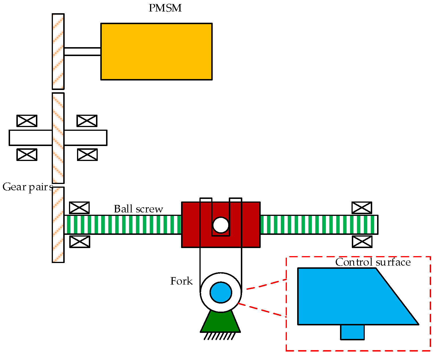
Consider a position servo system consisting of a permanent magnet synchronous motor driving a mechanical load through a ball screw transmission mechanism. The system configuration, illustrated in Figure 1, is representative of flight vehicle actuation systems where precise position control is required under varying load conditions. The mechanical dynamics of the system can be described by the following second-order differential equation:

$$J_{total}n\ddot{\theta }+Bn\dot{\theta }+T_f+T_l=K_t{i}_q$$

(1)

where $\theta$ is the angular position (rad) of the control surface, $J_{total}=J_m+J_l/n^2$ is the total equivalent inertia (kg·m²), $B$ is the viscous friction coefficient (N·m·s/rad), $T_f$ represents nonlinear friction torque (N·m), $T_l$ is the equivalent external load torque (N·m), $K_t$ is the motor torque constant (N·m/A), $i_q$ is the q-axis current, $n$ is the transmission ratio, $J_m$ is the motor inertia, and $J_l$ is the inertia of the control surface. All parameters $J_{total}$, $B$, $T_f$ and $T_l$ are all referred to the motor output shaft through the ball screw transmission ratio.

The nonlinear friction torque $T_f$ is modeled using a static Stribeck friction model [6,7], incorporating both Coulomb friction and velocity-dependent effects:

$$T_f=T_{c}sign(\dot{\theta })+T_s{e}^{-{\left|\dot{\theta }/{\omega }_s\right|}^2}sign(\dot{\theta })+B_v\dot{\theta }$$

(2)

where $T_c$ is the Coulomb friction torque, $T_s$ is the Stribeck friction amplitude, ${\omega }_s$ is the Stribeck velocity, and $B_v$ is the velocity-dependent friction.

Remark 1.

The static Stribeck model in (2) is chosen for its tractability in the observer-controller framework. The full LuGre model [7], which includes an internal bristle state governed by a first-order ODE, would provide more accurate friction characterization at low velocities but at the cost of increased observer dimensionality. At elevated temperatures (above approximately 200 °C), lubricant phase changes and thermal degradation may render both the static Stribeck and the dynamic LuGre models inaccurate [25] because LuGre bristle parameters are themselves calibrated for specific lubricant states. In the proposed framework, all such discrepancies, including unmodeled bristle transients during velocity reversals, enter the lumped disturbance $F(t)$ in the ultra-local model (Section 2.3). The LuGre bristle dynamics produce friction transients with time constants on the order of milliseconds during velocity reversals, placing them within the fast disturbance bandwidth estimated by the FTCESO.

2.2. Thermal Effects Modeling

High-speed flight vehicles experience extreme thermal loading during mission execution, with servo systems typically operating across temperatures from −55 °C to 250 °C. This section develops physically motivated models for temperature-dependent parameter variations.

2.2.1. Electromagnetic Parameter Variations

The temperature dependence of permanent magnet flux linkage follows a reversible demagnetization characteristic. The motor torque constant varies correspondingly as:

$$K_t(T)=K_{t0}(1-{\beta }_K\Delta T)$$

(3)

where $K_{t0}$ is the nominal torque constant at reference temperature $T_0$ (typically 20 °C), $\Delta T=T-T_0$ is the temperature deviation, and ${\beta }_K$ captures the thermal demagnetization effect, with typical values of 0.0008–0.0015/°C for NdFeB permanent magnet motors [26].

Remark 2.

The linear model (3) is valid in the reversible demagnetization regime, i.e., when $T\le T_{knee}$ (the knee-point temperature of the B-H curve). At temperatures approaching or exceeding $T_{knee}$, irreversible demagnetization occurs. In the proposed framework, irreversible demagnetization effects, should they occur gradually, manifest as a monotonically increasing bias in the lumped disturbance, which can be partially compensated by the slow-varying disturbance observer provided that the drift rate satisfies Assumption 4. However, sudden catastrophic demagnetization falls outside the scope of the present design.

2.2.2. Mechanical Parameter Variations

Temperature affects drivetrain equivalent inertia through thermal expansion. The moment of inertia variation can be approximated as [27,28]:

$$J_{total}(T)=J_0(1+{\beta }_J\Delta T)$$

(4)

where ${\beta }_J$ incorporates the effect of geometric expansion on rotational inertia.

The viscous damping coefficient varies due to lubricant viscosity changes following an Arrhenius-type exponential model [29]:

$$B(T)=B_0\exp \left(-{\beta }_B\Delta T\right)$$

(5)

where ${\beta }_B$ is the viscosity-temperature coefficient, reflecting the decrease in lubricant viscosity at elevated temperatures. As temperature increases, the lubricant viscosity decreases, reducing the effective viscous damping. This relationship is well-established in tribology literature for mineral oil and synthetic lubricants used in aerospace applications.

The friction parameters in Equation (2) exhibit strong temperature dependence arising from lubricant viscosity changes, thermal effects on contact surfaces, and bearing component expansion [25]:

$$T_f(T,\dot{\theta })=T_c(T)sign(\dot{\theta })+T_s(T)e^{-{\left|\dot{\theta }/{\omega }_s(T)\right|}^2}sign(\dot{\theta })+B_v(T)\dot{\theta }$$

(6)

where

$$\begin{gathered} T_c(T)=T_{C0}\left(1+{\beta }_{Tc}\Delta T\right) \\ T_s(T)=T_{s0}\exp \left(-{\beta }_{Ts}\Delta T\right) \\ {\omega }_s(T)={\omega }_{s0}\left(1+{\beta }_{\omega s}\Delta T\right) \\ B_v(T)=B_{v0}\exp \left(-{\beta }_{Bs}\Delta T\right) \end{gathered}$$

Remark 3.

The linear temperature dependence in (6) is a first-order approximation. At extreme temperatures, friction behavior involves phase changes in lubricants, surface oxidation, and boundary lubrication transitions that introduce nonlinear phenomena [25]. These higher-order effects are absorbed into the lumped disturbance term of the ultra-local model, ensuring that the control design remains robust without requiring precise high-temperature friction characterization.

2.3. Ultra-Local Model Formulation

To address the complexity arising from parameter uncertainties and thermal effects, we adopt an ultra-local model approach that reformulates the system dynamics without requiring detailed parameter knowledge during real-time operation.

2.3.1. System Reformulation

Starting from the mechanical dynamics Equation (1) with temperature-dependent parameters:

$$J_{total}(T)n\ddot{\theta }+B(T)n\dot{\theta }+T_f(T,\theta )+T_l=K_t(T)i_q$$

(7)

Dividing by the nominal inertia $J_0$ and defining the nominal control gain ${\alpha }_0={\displaystyle \frac{K_{t0}}{J_{0}n}}$, we obtain the ultra-local model representation:

$$\ddot{\theta }={\alpha }_0{i}_q+F(t)$$

(8)

where $F(t)$ is the lumped disturbance term encompassing all uncertainties and unmodeled dynamics.

2.3.2. Lumped Disturbance Decomposition

The lumped disturbance $F(t)$ can be explicitly expressed as:

$$F(t)=F_{param}(t)+F_{friction}(t)+F_{load}(t)+F_{gain}(t)$$

where each component is derived from the temperature-dependent system equations:

Parameters mismatch term:

$$F_{param}(t)=-{\displaystyle \frac{J_{total}(T)-J_0}{J_0}}\ddot{\theta }-{\displaystyle \frac{B(T)}{J_0}}\dot{\theta }$$

Friction term:

$$F_{friction}(t)=-{\displaystyle \frac{T_f(T,\dot{\theta })}{J_{0}n}}$$

External load term:

$$F_{load}(t)=-{\displaystyle \frac{T_l(t)}{J_{0}n}}$$

Control gain mismatch term:

$$F_{gain}(t)={\displaystyle \frac{K_t(T)-K_{t0}}{J_{0}n}}{i}_q$$

The lumped disturbance exhibits components varying on different time scales. Based on their temporal characteristics, we decompose:

$$F(t)=F_{fast}(t)+F_{slow}(t)$$

where the decomposition is defined based on a frequency-domain criterion. Let ${\omega }_c$ denote the cutoff frequency separating the fast and slow time scales. In practice, ${\omega }_c$ is selected based on the thermal time constant of the actuator system: ${\omega }_c=2\pi /(10{\tau }_{th})$, where ${\tau }_{th}$ is the dominant thermal time constant. The slow component $F_{slow}(t)$ contains spectral content below ${\omega }_c$, primarily comprising temperature-induced parameter drifts with time constants on the order of seconds to hundreds of seconds (${\tau }_{th}$ >> $1/{\omega }_c$). The fast component $F_{fast}(t)$ contains spectral content above ${\omega }_c$, including aerodynamic load variations, velocity-dependent friction variations, and high-frequency mechanical vibrations with time constants on the order of milliseconds (${\tau }_{mech}$ << $1/{\omega }_c$).

The thermal time constant ${\tau }_{th}$ is determined offline through thermal step-response testing of the actuator assembly. In this procedure, the actuator housing is subjected to a step change in ambient temperature, while the thermal response is recorded; the dominant time constant is extracted by fitting a first-order exponential model to the measured transient. This offline determination is justified because ${\tau }_{th}$ depends on the thermal mass and heat transfer geometry of the actuator, which are structural properties that remain approximately constant during operation. The factor of 10 in the denominator provides a conservative margin ensuring robust frequency separation even under variations in actual thermal dynamics.

2.4. Problem Statement and Control Objectives

The control objective is to design a position tracking controller such that the system output $\theta (t)$ follows a desired reference trajectory ${\theta }^{\ast }(t)$, with the following specifications:

• Finite-time convergence: The tracking error converges to a small residual set in finite time.
• Disturbance rejection: The controller effectively compensates for both fast-varying and slow-varying disturbances.
• Thermal adaptation: The control system adapts to temperature-induced parameter variations across the full operational range.

3. Dual-Layer Disturbance Observer Design

3.1. Observer Architecture Overview

The proposed dual-layer disturbance observer consists of two complementary estimation mechanisms:

• Third-order FTCESO: Estimates fast-varying disturbances $F_{fast}(t)$ with finite-time convergence.
• Adaptive slow observer: Estimates slowly varying thermal drifts $F_{slow}(t)$ using σ-modification adaptive techniques.

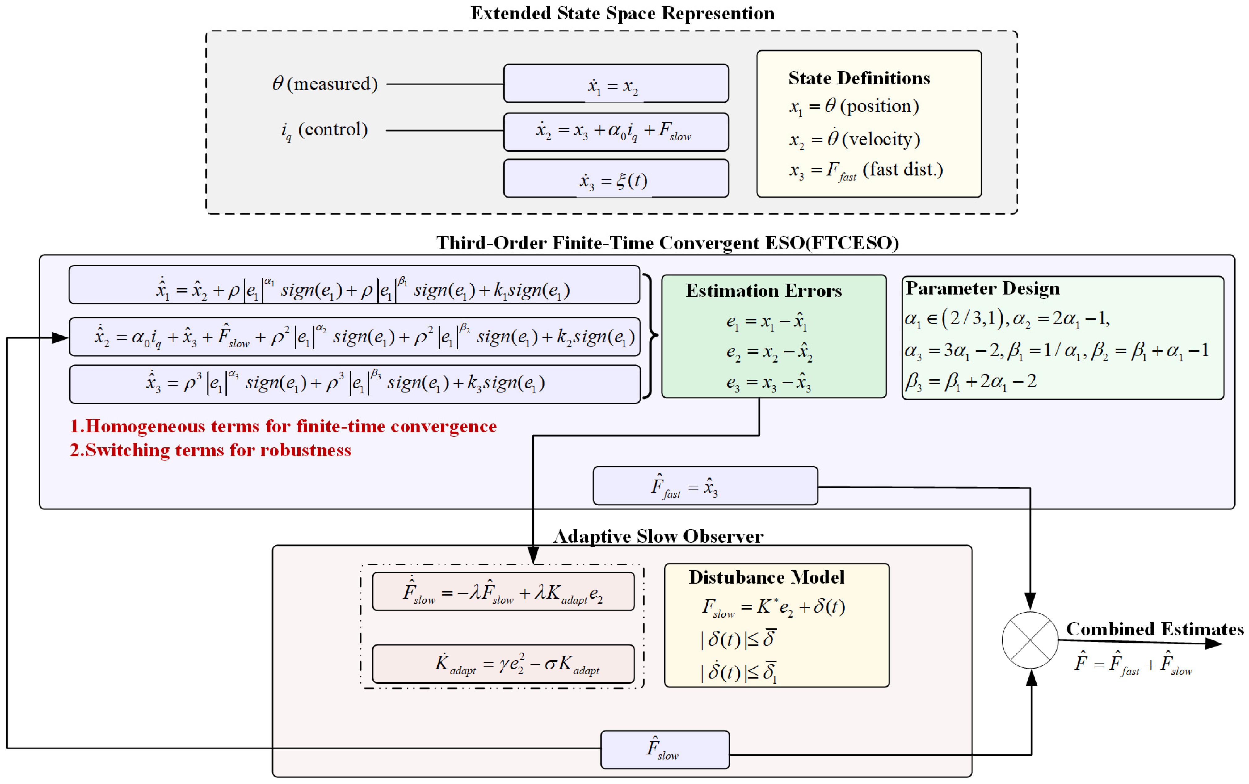
This architecture exploits the time-scale separation property identified in Section 2.3.2, allowing each observer layer to focus on disturbances within its optimal frequency range. The architecture of the dual-layer disturbance observer is depicted schematically in Figure 2.

3.2. Third-Order Finite-Time Convergent Extended State Observer

3.2.1. Third-Order Extended State Space Model

To facilitate observer design, we augment the system state space by treating the fast-varying disturbance as an additional state. Define state variables $x_1=\theta$, $x_2=\dot{\theta }$, and $x_3=F_{fast}$. The extended state-space representation becomes:

$$\left\{\begin{array}{l}{\dot{x}}_1=x_2\hfill \\ {\dot{x}}_2=x_3+{\alpha }_0{i}_q+F_{slow}\hfill \\ {\dot{x}}_3=\xi (t)\hfill \end{array}\right.$$

(9)

where $\xi (t)={\dot{F}}_{fast}(t)$ represents the time derivative of the fast-varying disturbance.

Assumption 1.

The disturbance $F_{fast}$ is continuously differentiable almost everywhere, with possible isolated discontinuities of the first kind.

Assumption 2.

The disturbance derivative $\xi (t)$ is unknown but bounded, i.e., $\left|\xi (t)\right|\le \overline{\xi }$, where $\overline{\xi }$ is a known positive constant.

3.2.2. Third-Order FTCESO Structure

Let ${\widehat{x}}_1$, ${\widehat{x}}_2$, and ${\widehat{x}}_3$ be the estimates of $x_1$, $x_2$, and $x_3$ respectively. The proposed third-order finite-time convergent ESO is:

$$\left\{\begin{array}{l}{\dot{\widehat{x}}}_1={\widehat{x}}_2+\rho {\left|e_1\right|}^{{\alpha }_1}sign(e_1)+\rho {\left|e_1\right|}^{{\beta }_1}sign(e_1)+k_{1}sign(e_1)\hfill \\ {\dot{\widehat{x}}}_2={\alpha }_0{i}_q+{\widehat{x}}_3+{\widehat{F}}_{slow}+{\rho }^2{\left|e_1\right|}^{{\alpha }_2}sign(e_1)+{\rho }^2{\left|e_1\right|}^{{\beta }_2}sign(e_1)+k_{2}sign(e_1)\hfill \\ {\dot{\widehat{x}}}_3={\rho }^3{\left|e_1\right|}^{{\alpha }_3}sign(e_1)+{\rho }^3{\left|e_1\right|}^{{\beta }_3}sign(e_1)+k_{3}sign(e_1)\hfill \end{array}\right.$$

(10)

where $e_1=x_1-{\widehat{x}}_1$ is the position estimation error; $\rho$ is the observer bandwidth parameter; $k_1$, $k_2$, and $k_3$ are switching gains; and ${\widehat{F}}_{slow}$ is the slow disturbance estimate from the adaptive observer. The exponential parameters are defined as follows:

$$\left\{\begin{array}{l}{\alpha }_1\in ({\displaystyle \frac{2}{3}},1),{\alpha }_2=2{\alpha }_1-1,{\alpha }_3=3{\alpha }_1-2\hfill \\ {\beta }_1={\displaystyle \frac{1}{{\alpha }_1}},{\beta }_2={\displaystyle \frac{1}{{\alpha }_1}}+{\alpha }_1-1,{\displaystyle \frac{1}{{\alpha }_1}}+2{\alpha }_1-2\hfill \end{array}\right.$$

(11)

3.2.3. Third-Order FTCESO Error Dynamics

Define the estimation errors:

$$e_1=x_1-{\widehat{x}}_1, e_2=x_2-{\widehat{x}}_2, e_3=x_3-{\widehat{x}}_3$$

The complete error system is

$$\left\{\begin{array}{l}{\dot{e}}_1=e_2-\rho |e_1{|}^{{\alpha }_1}sign(e_1)-\rho |e_1{|}^{{\beta }_1}sign(e_1)-k_{1}sign(e_1)\hfill \\ {\dot{e}}_2=e_3+{\tilde{F}}_{slow}-{\rho }^2|e_1{|}^{{\alpha }_2}sign(e_1)-{\rho }^2|e_1{|}^{{\beta }_2}sign(e_1)-k_{2}sign(e_1)\hfill \\ {\dot{e}}_3=\xi (t)-{\rho }^3|e_1{|}^{{\alpha }_3}sign(e_1)-{\rho }^3|e_1{|}^{{\beta }_3}sign(e_1)-k_{3}sign(e_1)\hfill \end{array}\right.$$

(12)

where ${\tilde{F}}_{slow}=F_{slow}-{\widehat{F}}_{slow}$ is the slow disturbance estimation error.

The error dynamics can be decomposed into four distinct components:

Component 1: Vector field $f_{\alpha }$:

$$f_{\alpha }=\left[\begin{array}{c}{e}_2-\rho |e_1{|}^{{\alpha }_1}sign(e_1)\\ e_3-{\rho }^2|e_1{|}^{{\alpha }_2}sign(e_1)\\ -{\rho }^3|e_1{|}^{{\alpha }_3}sign(e_1)\end{array}\right]$$

(13)

Component 2: Vector field $f_{\beta }$:

$$f_{\beta }=\left[\begin{array}{c}-\rho |e_1{|}^{{\beta }_1}sign(e_1)\\ -{\rho }^2|e_1{|}^{{\beta }_2}sign(e_1)\\ -{\rho }^3|e_1{|}^{{\alpha }_3}sign(e_1)\end{array}\right]$$

(14)

Component 3: Switching terms $f_s$:

$$f_s=\left[\begin{array}{c}-k_{1}sign(e_1)\\ -k_{2}sign(e_1)\\ -k_{3}sign(e_1)\end{array}\right]$$

(15)

Component 4: Disturbance terms $d$:

$$d=\left[\begin{array}{c}0\\ {\tilde{F}}_{slow}\\ \xi (t)\end{array}\right]$$

(16)

The complete system representation is

$$\dot{e}=f_{\alpha }+f_{\beta }+f_s+d$$

(17)

where $e=(e_1,e_2,e_3)$.

Remark 4.

By homogeneity theory [30,31,32], assigning weights $r_1=1$, $r_2={\alpha }_1$, and $r_3=2{\alpha }_1-1$ to the state components $e_1,e_2,e_3$ respectively, the vector fields have the following homogeneity degrees with respect to the dilation ${\Delta }_{\lambda }^r(e)=({\lambda }^{r_1}{e}_1,{\lambda }^{r_2}{e}_2,{\lambda }^{r_3}{e}_3)$:

• $f_{\alpha }$ has negative homogeneity degree ${\tau }_{\alpha }={\alpha }_1-1<0$ (dominant for small errors, providing finite-time convergence);
• $f_{\beta }$ has positive homogeneity degree ${\tau }_{\beta }={\beta }_1-1>0$ (dominant for large errors, ensuring global convergence).

3.3. Slow-Varying Disturbance Observer Design

We present the slow-varying disturbance observer before the FTCESO convergence analysis, as the slow observer stability result is required in the FTCESO convergence proof.

3.3.1. Slow-Varying Disturbance Model

The slow-varying disturbance, which captures temperature-induced parameter drifts including viscous damping variations and torque constant drift, is modeled as:

$$F_{slow}=K^{\ast }{e}_2+\delta (t)$$

(18)

where $K^{\ast }$ is the ideal unknown gain parameter representing the coupling between velocity error and thermal drift, $\delta (t)$ is a bounded residual term satisfying $|\delta (t)|\le \overline{\delta }$, and $e_2=\dot{\theta }-\dot{\widehat{\theta }}$ is the velocity estimation error from FTCESO. The parameter $K^{\ast }$ aggregates the velocity-coupled thermal drift effects (primarily $\Delta B(T)/J_0$), where $\Delta B(T)=B(T)-B_0$ represents the temperature-induced change in viscous damping. The residual $\delta (t)$ captures remaining terms including the torque constant drift and higher-order effects.

3.3.2. Adaptive Observer Dynamics

The slow-varying disturbance observer employs an adaptive estimation approach with low-pass filtering characteristics:

$$\left\{\begin{array}{c}{\dot{\widehat{F}}}_{slow}=-\lambda {\widehat{F}}_{slow}+\lambda K_{adapt}{e}_2\\ {\dot{K}}_{adapt}=\gamma e_2^2-\sigma K_{adapt}\end{array}\right.$$

(19)

where $\lambda$ is the filter bandwidth, $\gamma >0$ is the adaptation gain, and $\sigma >0$ provides $\sigma$-modification for robustness [33]. The low-pass characteristic ensures that the slow observer does not attempt to track fast disturbances.

Assumption 3 (Boundedness of ${\mathit{e}}_{\mathbf{2}}$).

The velocity estimation error from FTCESO satisfies $\left|e_2\right|\le {\overline{e}}_2$, with ${\overline{e}}_2$ being a small positive constant determined by the FTCESO residual set.

Assumption 4 (Slow variation).

The residual $\delta (t)$ satisfies $|\dot{\delta }(t)|\le {\overline{\delta }}_1$, consistent with the thermal drift time scale.

Define estimation error ${\tilde{F}}_{slow}=F_{slow}-{\widehat{F}}_{slow}$ and $\tilde{K}=K_{adapt}-K^{\ast }$.

From (18) and (19):

$${\dot{\tilde{F}}}_{slow}={\dot{F}}_{slow}-{\dot{\widehat{F}}}_{slow}=-\lambda {\tilde{F}}_{slow}-\lambda \tilde{K}{e}_2+K^{\ast }{\dot{e}}_2+\dot{\delta }(t)+\lambda \delta (t)=-\lambda {\tilde{F}}_{slow}-\lambda \tilde{K}{e}_2+w(t)$$

(20)

where $w(t)=K^{\ast }{\dot{e}}_2+\dot{\delta }(t)+\lambda \delta (t)$.

Under quasi-steady-state operation, where $\left|{\dot{e}}_2\right|$ is negligible, justified by the time-scale separation between FTCESO and slow observer, we have

$$\left|w(t)\right|\le =\overline{w}=\lambda \overline{\delta }+{\overline{\delta }}_1$$

3.3.3. Stability Analysis of the Slow Observer

Consider the Lyapunov function:

$$V_{slow}={\displaystyle \frac{1}{2}}{\tilde{F}}_{slow}^2+{\displaystyle \frac{1}{2\gamma }}{\tilde{K}}^2$$

(21)

Theorem 1.

Under Assumptions 3 and 4, if the design parameters satisfy:

$$\sigma >{\displaystyle \frac{2\gamma (1+\lambda {\overline{e}}_2^2)}{3}}$$

(22)

Then the slow observer system (19) achieves practical stability with the following properties:

1. Exponential convergence: The Lyapunov function satisfies:

$$V_{slow}(t)\le V_{slow}(0)e^{-{\mu }_{5}t}+{\displaystyle \frac{D}{{\mu }_5}}(1-e^{-{\mu }_{5}t})$$

where $V_{slow}(0)={\displaystyle \frac{1}{2}}{\tilde{F}}_{slow}^2(0)+{\displaystyle \frac{1}{2\gamma }}{\tilde{K}}_{slow}^2(0)$.

2. Finite settling time: For any ${\epsilon }_s>0$, define the settling time:

$$T_s({\epsilon }_s)={\displaystyle \frac{1}{{\mu }_5}}\ln \left({\displaystyle \frac{V_{slow}(0)}{{\epsilon }_s}}\right)$$

Then, for all $t\ge T_s({\epsilon }_s)$:

$$\left|{\tilde{F}}_{slow}(t)\right|\le \sqrt{{\displaystyle \frac{2D}{{\mu }_5}}}+\delta ({\epsilon }_s)$$

where ${\mu }_5=\min \left\{\begin{array}{cc}{\displaystyle \frac{\lambda }{2}}& {\displaystyle \frac{3}{2}}\sigma -\gamma (1+\lambda {\overline{e}}_2^2)\end{array}\right\}$ and $D$ is a bounded constant.

Proof of Theorem 1.

From (20) and (21):

$${\dot{V}}_{slow}={\dot{\tilde{F}}}_{slow}{\tilde{F}}_{slow}+{\displaystyle \frac{1}{\gamma }}\tilde{K}\dot{\tilde{K}}=-\lambda {\tilde{F}}_{slow}^2-{\displaystyle \frac{\sigma }{\gamma }}{\tilde{K}}^2+\tilde{K}{e}_2^2-\lambda {\tilde{F}}_{slow}\tilde{K}{e}_2+{\tilde{F}}_{slow}w(t)-{\displaystyle \frac{\sigma K^{\ast }}{\gamma }}\tilde{K}$$

(23)

Using Young’s inequality $ab\le {\displaystyle \frac{{\epsilon }_y{a}^2}{2}}+{\displaystyle \frac{b^2}{2{\epsilon }_y}}$ with appropriate free parameters ${\epsilon }_y>0$, we can get:

$$\tilde{K}{e}_2^2\le \tilde{K}{\overline{e}}_2^2\le {\displaystyle \frac{{\tilde{K}}^2}{2}}+{\displaystyle \frac{{\overline{e}}_2^4}{2}}$$

(24)

$$-\lambda {\tilde{F}}_{slow}\tilde{K}{e}_2\le \lambda \left|{\tilde{F}}_{slow}\right|\left|\tilde{K}\right|{\overline{e}}_2\le {\displaystyle \frac{\lambda {\tilde{F}}_{slow}^2}{2}}+{\displaystyle \frac{\lambda {\overline{e}}_2^2{\tilde{K}}^2}{2}}$$

(25)

$${\tilde{F}}_{slow}w(t)\le {\displaystyle \frac{\lambda }{4}}{\tilde{F}}_{slow}^2+{\displaystyle \frac{1}{\lambda }}{\overline{w}}^2$$

(26)

$$-{\displaystyle \frac{\sigma K^{\ast }}{\gamma }}\tilde{K}\le {\displaystyle \frac{\sigma }{4\gamma }}{\tilde{K}}^2+{\displaystyle \frac{\sigma {(K^{\ast })}^2}{\gamma }}$$

(27)

Substituting (24)–(27) into (23):

$${\dot{V}}_{slow}\le -{\displaystyle \frac{\lambda {\tilde{F}}_{slow}^2}{4}}-({\displaystyle \frac{3\sigma }{4\gamma }}-{\displaystyle \frac{1+\lambda {\overline{e}}_2^2}{2}}){\tilde{K}}^2+{\displaystyle \frac{{\overline{e}}_2^4}{2}}+{\displaystyle \frac{{\overline{w}}^2}{\lambda }}+{\displaystyle \frac{\sigma {(K^{\ast })}^2}{\gamma }}$$

(28)

Define ${\mu }_3={\displaystyle \frac{\lambda }{4}}$, ${\mu }_4={\displaystyle \frac{3\sigma }{4\gamma }}-{\displaystyle \frac{1+\lambda {\overline{e}}_2^2}{2}}$, $D={\displaystyle \frac{{\overline{e}}_2^4}{2}}+{\displaystyle \frac{{\overline{w}}^2}{\lambda }}+{\displaystyle \frac{\sigma {(K^{\ast })}^2}{\gamma }}$

For the coefficient of ${\tilde{K}}^2$ to be positive ensuring decay, we require

$${\displaystyle \frac{3\sigma }{4\gamma }}-{\displaystyle \frac{1+\lambda {\overline{e}}_2^2}{2}}>0$$

This yields the sufficient condition

$$\sigma >{\displaystyle \frac{2\gamma (1+\lambda {\overline{e}}_2^2)}{3}}$$

Then, from (28):

$${\dot{V}}_{slow}\le -{\mu }_3{\tilde{F}}_{slow}^2-{\mu }_4{\tilde{F}}_{slow}^2{\tilde{K}}^2+D=-2{\mu }_3·{\displaystyle \frac{1}{2}}{\tilde{F}}_{slow}^2-2\gamma {\mu }_4·{\displaystyle \frac{1}{2\gamma }}{\tilde{F}}_{slow}^2{\tilde{K}}^2+D\le -{\mu }_5{V}_{slow}+D$$

(29)

where ${\mu }_5=\min (2{\mu }_3,2\gamma {\mu }_4)=\min ({\displaystyle \frac{\lambda }{2}},{\displaystyle \frac{3\sigma }{2}}-\gamma (1+\lambda {\overline{e}}_2^2))$.

When $V_{slow}\ge {\displaystyle \frac{D}{{\mu }_5}}$, ${\dot{V}}_{slow}\le 0$.

Therefore, the estimation errors $({\tilde{F}}_{slow},\tilde{K})$ converge to a residual set characterized by:

$$\mathsf{\Omega }=\left\{({\tilde{F}}_{slow},\tilde{K}):V({\tilde{F}}_{slow},\tilde{K})\le {\displaystyle \frac{D}{{\mu }_5}}\right\}$$

For thermal drift applications, ${\overline{\delta }}_1$ << $\lambda \overline{\delta }$ (slowly varying), and $\overline{e}$ is small (due to FTCESO high-bandwidth tracking); the dominant contribution in $D$ becomes:

$$D={\displaystyle \frac{{\overline{e}}_2^4}{2}}+{\displaystyle \frac{{(\lambda \overline{\delta }+{\overline{\delta }}_1)}^2}{\lambda }}+{\displaystyle \frac{\sigma {(K^{\ast })}^2}{\gamma }}\approx \lambda {\overline{\delta }}^2+{\displaystyle \frac{\sigma {(K^{\ast })}^2}{\gamma }}$$

Selecting $\lambda$ small maintain low-pass characteristics reduces the first term, while choosing ${\displaystyle \frac{\sigma }{\gamma }}$ appropriately reduces the second term, and the residual set $\mathsf{\Omega }$ can be made sufficiently small.

From (29), by the Comparison Lemma:

$$V_{slow}(t)\le V_{slow}(0)e^{-{\mu }_{5}t}+{\displaystyle \frac{D}{{\mu }_5}}(1-e^{-{\mu }_{5}t})$$

For $t\ge T_s({\epsilon }_s)={\displaystyle \frac{1}{{\mu }_5}}\ln \left({\displaystyle \frac{V_{slow}(0)}{{\epsilon }_s}}\right)$, $e^{-{\mu }_{5}t}\le e^{-{\mu }_5{t}_s}={\displaystyle \frac{{\epsilon }_s}{V_{slow}(0)}}$

Therefore,

$$V_{slow}(t)\le V_{slow}(0){\displaystyle \frac{{\epsilon }_s}{V_{slow}(0)}}+{\displaystyle \frac{D}{{\mu }_5}}(1-e^{-{\mu }_{5}t})={\epsilon }_s+{\displaystyle \frac{D}{{\mu }_5}}$$

We can get:

$$\left|{\tilde{F}}_{slow}(t)\right|\le \sqrt{2V_{slow}(t)}\le \sqrt{{\displaystyle \frac{2D}{{\mu }_5}}+2{\epsilon }_s}$$

Define $\delta ({\epsilon }_s)=\sqrt{{\displaystyle \frac{2D}{{\mu }_5}}+2{\epsilon }_s}-\sqrt{{\displaystyle \frac{2D}{{\mu }_5}}}$.

By continuity, $\delta ({\epsilon }_s)\to 0$ as ${\epsilon }_s\to 0$.

For $t\ge T_s({\epsilon }_s)$:

$$\left|{\tilde{F}}_{slow}(t)\right|\le \sqrt{{\displaystyle \frac{2D}{{\mu }_5}}}+\delta ({\epsilon }_s)$$

This completes the proof of Theorem 1. $\square$

3.4. Finite-Time Convergence Analysis of the FTCESO

We now establish the convergence properties of the FTCESO, utilizing the slow observer result from Theorem 1.

Define the transformed coordinates:

$$\overline{e}=\left[\begin{array}{c}|e_1{|}^{1/\varphi } sign(e_1)\\ |e_2{|}^{1/(\varphi {\alpha }_1)} sign(e_2)\\ |e_3{|}^{1/(\varphi {\alpha }_2)} sign(e_3)\end{array}\right]$$

(30)

where $\varphi ={\alpha }_1{\alpha }_2{\alpha }_3$.

Define the Lyapunov function:

$$V(e)={\overline{e}}^{T}P\overline{e}=p_1{\overline{e}}_1^2+p_2{\overline{e}}_2^2+p_3{\overline{e}}_3^2$$

(31)

where $P=diag(p_1,p_2,p_3)$ with $p_1$, $p_2$, and $p_3>0$.

Lemma 1.

Consider the slow observer system (19) with initial conditions ${\widehat{F}}_{slow}(0)$, and $K_{slow}(0)$. Under Assumption 4 and condition (22), for all $t\ge 0$,

$$\left|{\tilde{F}}_{slow}(t)\right|\le \sqrt{2V_{slow}(0)}+\sqrt{{\displaystyle \frac{2D}{{\mu }_5}}}=M_{slow}$$

Proof of Lemma 1.

From the slow observer Lyapunov analysis in Theorem 1, we have

$$V_{slow}(t)\le V_{slow}(0)e^{-{\mu }_{5}t}+{\displaystyle \frac{D}{{\mu }_5}}(1-e^{-{\mu }_{5}t})$$

Since $e^{-{\mu }_{5}t}\le 1$ and $1-e^{-{\mu }_{5}t}\le 1$ for $t\ge 0$:

$$V_{slow}(t)\le V_{slow}(0)+{\displaystyle \frac{D}{{\mu }_5}}$$

From ${\displaystyle \frac{1}{2}}{\widehat{F}}_{slow}^2\le V_{slow}$:

$$\left|{\tilde{F}}_{slow}(t)\right|\le \sqrt{2V_{slow}(0)+{\displaystyle \frac{2D}{{\mu }_5}}}\le \sqrt{2V_{slow}(0)}+\sqrt{{\displaystyle \frac{2D}{{\mu }_5}}}=M_{slow}$$

This bound holds uniformly for all $t\ge 0$. $\square$

Theorem 2.

Consider the error system (12). Under Assumptions 1 and 2, for sufficiently large $\rho$ and properly chosen switching gains $k_i$, the estimation errors $(e_1,e_2,e_3)$ converge to a residual set $\Re =\left\{e:V(e)\le V_{res}\right\}$ in finite time, followed by exact convergence to zero via switching terms.

Proof of Theorem 2.

From (30) and (31):

$$V(e)=p_1{\left|e_1\right|}^{2/\varphi }+p_2{\left|e_2\right|}^{2/(\varphi {\alpha }_1)}+p_3{\left|e_3\right|}^{2/(\varphi {\alpha }_2)}$$

(32)

The gradients with respect to $e$ are computed as

$$\left\{\begin{array}{l}{\displaystyle \frac{\partial V}{\partial e_1}}={\displaystyle \frac{2p_1}{\varphi }}{\left|e_1\right|}^{2/\varphi -1}sign(e_1)\hfill \\ {\displaystyle \frac{\partial V}{\partial e_2}}={\displaystyle \frac{2p_2}{\varphi {\alpha }_1}}{\left|e_1\right|}^{2/(\varphi {\alpha }_1)-1}sign(e_2)\hfill \\ {\displaystyle \frac{\partial V}{\partial e_3}}={\displaystyle \frac{2p_3}{\varphi {\alpha }_2}}{\left|e_3\right|}^{2/(\varphi {\alpha }_2)-1}sign(e_3)\hfill \end{array}\right.$$

(33)

From (33), the time derivative of $V(e)$ is

$$\dot{V}={\displaystyle \frac{\delta V}{\delta \overline{e}}}{\displaystyle \frac{\delta \overline{e}}{\delta t}}={\displaystyle \frac{\delta V}{\delta e}}{\displaystyle \frac{\delta e}{\delta \overline{e}}}{\displaystyle \frac{\delta \overline{e}}{\delta e}}{\displaystyle \frac{de}{dt}}={\displaystyle \frac{\delta V}{\delta e}}\dot{e}=L_{f_{\alpha }}V+L_{f_{\beta }}V+L_{f_s}V+L_{d}V$$

(34)

where $L_{f_i}V$ denotes the Lie derivative of $V$ along the vector field $f_i$.

By homogeneity theory [30,31,32], the Lie derivatives $L_{f_{\alpha }}V$ and $L_{f_{\beta }}V$ satisfy:

$$L_{f_{\alpha }}V\le -{\mu }_1{V}^{{\gamma }_1}$$

(35)

$$L_{f_{\beta }}V\le -{\mu }_2{V}^{{\gamma }_2}$$

(36)

where

$${\gamma }_1=1+{\displaystyle \frac{\varphi ({\alpha }_1-1)}{2}}<1, {\gamma }_2=1+{\displaystyle \frac{\varphi (1-{\alpha }_1)}{2{\alpha }_1}}>1$$

$${\mu }_1=-\underset{\left\{e:V(e)=1\right\}}{\max }{L}_{f_{\alpha }}V(e), {\mu }_2=-\underset{\left\{e:V(e)=1\right\}}{\max }{L}_{f_{\beta }}V(e)$$

${\mu }_1$ and ${\mu }_2>0$ are constants that increase with the observer bandwidth parameter $\rho$.

According to (15), (16) and (33), $L_{f_s}V$ and $L_{f_d}V$ are computed as follows:

$$\begin{array}{l}{L}_{f_s}V\le -{\displaystyle \frac{2k_1{p}_1{({\left|{\overline{e}}_1\right|}^{\varphi })}^{2/\varphi -1}}{\varphi }}+{\displaystyle \frac{2k_2{p}_2{({\left|{\overline{e}}_2\right|}^{\varphi {\alpha }_1})}^{2/(\varphi {\alpha }_1)-1}}{\varphi {\alpha }_1}}+{\displaystyle \frac{2k_3{p}_3{({\left|{\overline{e}}_3\right|}^{\varphi {\alpha }_2})}^{2/(\varphi {\alpha }_2)-1}}{\varphi {\alpha }_2}}\\ =-{\displaystyle \frac{2k_1{p}_1{\left|{\overline{e}}_1\right|}^{2-\varphi }}{\varphi }}+{\displaystyle \frac{2k_2{p}_2{\left|{\overline{e}}_2\right|}^{2-\varphi {\alpha }_1}}{\varphi {\alpha }_1}}+{\displaystyle \frac{2k_3{p}_3{\left|{\overline{e}}_3\right|}^{2-\varphi {\alpha }_2}}{\varphi {\alpha }_2}}\end{array}$$

(37)

$$\begin{array}{l}{L}_{f_d}V={\displaystyle \frac{2p_2}{\varphi {\alpha }_1}}{\left|e_1\right|}^{2/(\varphi {\alpha }_1)-1} sign(e_2){\tilde{F}}_{slow}+{\displaystyle \frac{2p_3\xi (t){\left|e_3\right|}^{2/(\varphi {\alpha }_2)-1}}{\varphi {\alpha }_2}}sign(e_3)\\ \le {\displaystyle \frac{2p_2{M}_{slow}}{\varphi {\alpha }_1}}{\left|e_1\right|}^{2/(\varphi {\alpha }_1)-1}+{\displaystyle \frac{2p_3\overline{\xi }{\left|e_3\right|}^{2/(\varphi {\alpha }_2)-1}}{\varphi {\alpha }_2}}\end{array}$$

(38)

Substituting Equations (35)–(38) into (34),

$$\begin{array}{l}\dot{V}\le -{\mu }_1{V}^{{\gamma }_1}-{\mu }_2{V}^{{\gamma }_2}-{\displaystyle \frac{2k_1{p}_1}{\varphi p_1^{1-\varphi /2}}}{V}^{1-\varphi /2}+{\displaystyle \frac{2k_2{p}_2+2p_2{M}_{slow}}{\varphi {\alpha }_1{p}_2^{1-\varphi {\alpha }_1/2}}}{V}^{1-\varphi {\alpha }_1/2}+{\displaystyle \frac{2k_3{p}_3+2p_3\overline{\xi }}{\varphi {\alpha }_2{p}_3^{1-\varphi {\alpha }_1/2}}}{V}^{1-\varphi {\alpha }_2/2}\\ =-{\mu }_1{V}^{{\gamma }_1}-{\mu }_2{V}^{{\gamma }_2}+C_1{V}^{{\upsilon }_1}+C_2{V}^{{\upsilon }_2}\end{array}$$

(39)

where ${\upsilon }_1=1-{\displaystyle \frac{\varphi {\alpha }_1}{2}}$, ${\upsilon }_2=1-{\displaystyle \frac{\varphi {\alpha }_2}{2}}$, $C_1={\displaystyle \frac{2k_2{p}_2+2p_2{M}_{slow}}{\varphi {\alpha }_1{p}_2^{1-\varphi {\alpha }_1/2}}}$, $C_2={\displaystyle \frac{2k_3{p}_3+2p_3\overline{\xi }}{\varphi {\alpha }_2{p}_3^{1-\varphi {\alpha }_1/2}}}$.

According to (11),

$${\upsilon }_1<{\upsilon }_2<{\gamma }_1<1<{\gamma }_2$$

Let $\dot{V}=0$ to derivate the residual $V_{res}$.

$$-{\mu }_1{V}^{{\gamma }_1}-{\mu }_2{V}^{{\gamma }_2}+C_1{V}^{{\upsilon }_1}+C_2{V}^{{\upsilon }_2}=0$$

For sufficiently small $V$, $V^{{\upsilon }_1}$ is the largest term, and $V^{{\gamma }_2}$ is the smallest. The primary balance occurs between terms with adjacent exponents.

$${\mu }_1{V}^{{\gamma }_1}\approx C_1{V}^{{\upsilon }_1}+C_2{V}^{{\upsilon }_2}$$

Since $V$ is small and ${\upsilon }_1-{\upsilon }_2$ is small,

$$V_{res}={\left({\displaystyle \frac{C_1+C_2}{{\mu }_1}}\right)}^{{\displaystyle \frac{1}{{\gamma }_1-{\upsilon }_1}}}$$

The residual decreases exponentially as the ratio ${\displaystyle \frac{C_1+C_2}{{\mu }_1}}$ decreases, since ${\mu }_1$ is increased with $\rho$. When $\rho$ is big enough, the residual can be sufficiently small.

From (39),

$$\dot{V}\le V^{{\gamma }_1}(-{\mu }_1-{\mu }_2{V}^{{\gamma }_2-{\gamma }_1}+C_1{V}^{{\upsilon }_1-{\gamma }_1}+C_2{V}^{{\upsilon }_2-{\gamma }_1})$$

As $V$ increases above $V_{res}$, the ${\mu }_2{V}^{{\gamma }_2-{\upsilon }_1}$ term increases, the $C_1{V}^{{\upsilon }_1-{\gamma }_1}$ and $C_2{V}^{{\upsilon }_2-{\gamma }_1}$ terms decrease, and then $-{\mu }_1-{\mu }_2{V}^{{\gamma }_2-{\gamma }_1}+C_1{V}^{{\upsilon }_1-{\gamma }_1}+C_2{V}^{{\upsilon }_2-{\gamma }_1}$ is strictly decreasing.

For $V\ge V_{res}$, we have $\dot{V}<0$ and:

$$\dot{V}\le -{\mu }_{eff}{V}^{{\gamma }_1}$$

(40)

where ${\mu }_{eff}={\min }_{V\in \left[V_{res},V_{\max }\right]}h(V)>0$ with

$$h(V)={\mu }_1+{\mu }_2{V}^{{\gamma }_2-{\gamma }_1}-C_1{V}^{{\upsilon }_1-{\gamma }_1}-C_2{V}^{{\upsilon }_2-{\gamma }_1}$$

Integrating (40) from initial $V_0$ to $V_{res}$:

$${\displaystyle {\int }_{V_0}^{V_{res}}{V}^{-{\gamma }_1}}dV\le -{\mu }_{eff}{\displaystyle {\int }_0^{T}dt}$$

We can get the convergence time to a residual set $\Re =\left\{e:V(e)\le V_{res}\right\}$:

$$T_f\le {\displaystyle \frac{V_0^{1-{\gamma }_1}-V_{res}^{1-{\gamma }_1}}{{\mu }_{eff}(1-{\gamma }_1)}}$$

After the observer reaches the residual set $\Re$:

$$p_1{\left|e_1\right|}^{2/\varphi }+p_2{\left|e_2\right|}^{2/(\varphi {\alpha }_1)}+p_3{\left|e_3\right|}^{2/(\varphi {\alpha }_2)}=V_{res}$$

The errors $e_1$, $e_2$ and $e_3$ satisfy

$$\left|e_1\right|\le {\chi }_1, \left|e_2\right|\le {\chi }_2, \left|e_3\right|\le {\chi }_3$$

where ${\chi }_1$, ${\chi }_2$ and ${\chi }_3>0$ are constants determined by $V_{res}$.

Define $V_1={\displaystyle \frac{1}{2}}{e}_1^2$:

$${\dot{V}}_1\le {\chi }_2\left|e_1\right|-\rho |e_1{|}^{{\alpha }_1+1}-\rho |e_1{|}^{{\beta }_1+1}-k_1\left|e_1\right|=-\rho |e_1{|}^{{\alpha }_1+1}-\rho |e_1{|}^{{\beta }_1+1}-\left|e_1\right|(k_1-{\chi }_2)$$

Choose $k_1>{\chi }_2$:

$${\dot{V}}_1=e_1{\dot{e}}_1\le -\rho |e_1{|}^{{\alpha }_1+1}-\rho |e_1{|}^{{\beta }_1+1}\le -2\rho |e_1{|}^{\frac{{\alpha }_1+{\beta }_1+2}{2}}$$

(41)

Denote $n_1={\displaystyle \frac{{\alpha }_1+{\beta }_1}{2}}$, integrating (41) from $e_1(T_f)$ to 0, the convergence time of $e_1$:

$$T_3\le {\displaystyle \frac{{[e_1(T_f)]}^{1-n_1}}{2\rho (1-n_1)}}\le {\displaystyle \frac{{\chi }_1^{1-n_1}}{2\rho (1-n_1)}}$$

In the same way, $e_2$ converges to zero in finite time $T_4$ with $k_2>{\chi }_3$, and $e_3$ converges to zero in finite time $T_5$ respectively with $k_3>\overline{\xi }$.

The total convergence time $T_{ob}=T_f+T_3++T_4++T_5$. $\square$

4. Adaptive Sliding Mode Control Design

4.1. Global Nonlinear Integral Terminal Sliding Surface

To achieve finite-time convergence with superior transient and steady-state performance, we design a global nonlinear integral terminal sliding surface.

Define the position tracking error:

$$e_p={\theta }^{\ast }-\theta , {\dot{e}}_p={\dot{\theta }}^{\ast }-\dot{\theta }, {\ddot{e}}_p={\ddot{\theta }}^{\ast }-\ddot{\theta }$$

(42)

The proposed global nonlinear integral terminal sliding surface is:

$$s=c_1{e}_p+{\dot{e}}_p+c_2{\displaystyle {\int }_0^t{e}_{p}d\tau }+c_3{\left({\displaystyle {\int }_0^t{e}_{p}d\tau }\right)}^{q/p}$$

(43)

where $c_1$, $c_2$, and $c_3>0$ are design parameters providing design flexibility for tuning transient response, $1<{\displaystyle \frac{q}{p}}<2$ is the terminal exponent, and $p$ and $q$ are both odd positive integers.

Taking the derivative of (43):

$$\dot{s}=c_1{\dot{e}}_p+{\ddot{e}}_p+c_2{e}_p+c_3{\displaystyle \frac{q}{p}}{e}_p{\left({\displaystyle {\int }_0^t{e}_{p}d\tau }\right)}^{q/p-1}$$

(44)

Substituting the error dynamics from (42) and using the system dynamics Equation (8):

$$\dot{s}={\ddot{\theta }}^{\ast }-{\alpha }_0{i}_q-F+c_1{\dot{e}}_p+c_2{e}_p+c_3{\displaystyle \frac{q}{p}}{e}_p{\left({\displaystyle {\int }_0^t{e}_{p}d\tau }\right)}^{q/p-1}$$

(45)

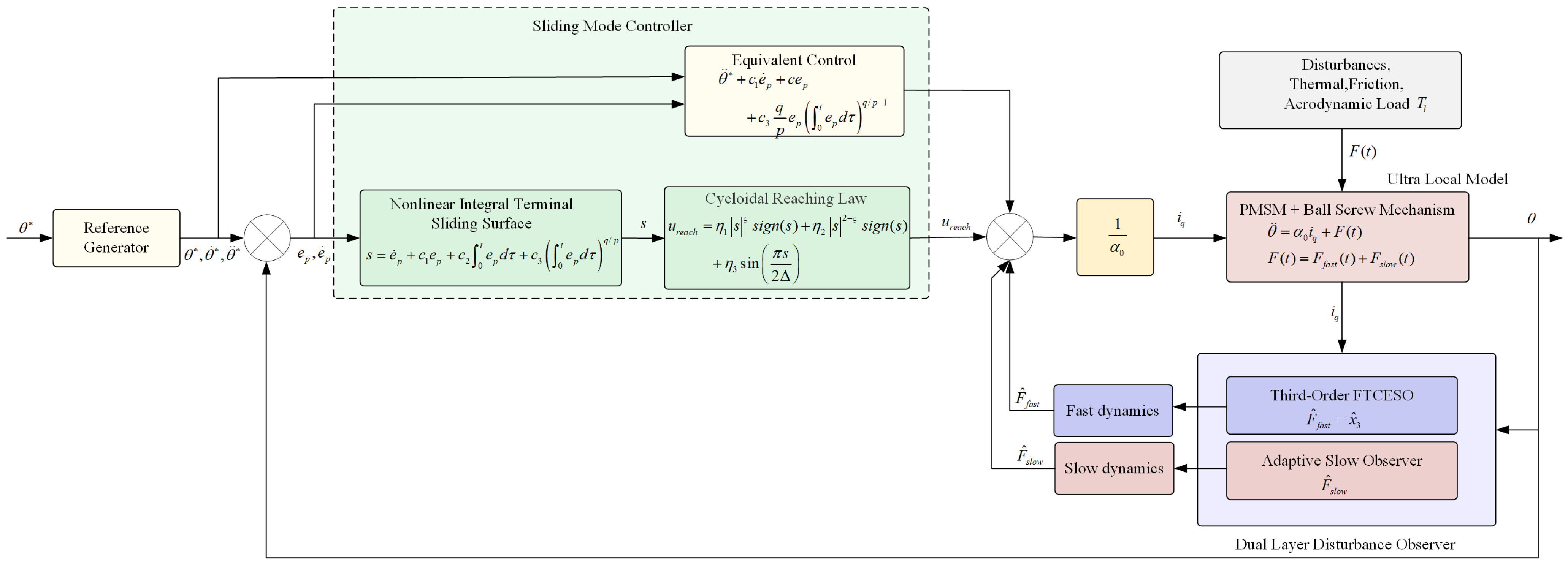
To achieve robust sliding mode control with chattering suppression, we employ a novel cycloidal reaching law:

$$u_{reach}={\eta }_1{\left|s\right|}^{\varsigma } sign(s)+{\eta }_2{\left|s\right|}^{2-\varsigma } sign(s)+{\eta }_3\sin \left({\displaystyle \frac{\pi s}{2\Delta }}\right)$$

(46)

where ${\eta }_1$, ${\eta }_2$, and ${\eta }_3>0$ are reaching law gains, $0<\varsigma <1$ determines convergence rate near equilibrium, and $\Delta$ is the boundary layer thickness.

The cycloidal term $\sin \left({\displaystyle \frac{\pi s}{2\Delta }}\right)$ provides smooth transition through the sliding surface, bounded control effort and effective chattering suppression.

Remark 5.

The boundary layer thickness $\mathsf{\Delta }$ in the cycloidal reaching law (46) introduces a design trade-off that is analyzed below.

• Boundary-layer trade-off analysis. Within the boundary layer $\left|s\right|\le \Delta$, the cycloidal term provides a smooth, bounded control contribution with maximum amplitude ${\eta }_3$. The chattering amplitude in steady state is bounded by ${\eta }_3\sin {\displaystyle \frac{\pi {\Delta }_{eff}}{2\Delta }}$, where ${\Delta }_{eff}\le \Delta$ is the effective switching band determined by the sampling period and sensor noise. Increasing Δ reduces this bound, yielding smoother control. Crucially, from Theorem 3, the residual sliding variable $s^{\ast }={\left({\displaystyle \frac{\overline{\epsilon }+{\epsilon }_0+{\eta }_3}{{\eta }_1}}\right)}^{1/\varsigma }$ and ultimate tracking error ${\epsilon }_{track}={\displaystyle \frac{s^{\ast }}{c_1}}+{\displaystyle \frac{2(\overline{\epsilon }+{\epsilon }_0)+{\overline{\epsilon }}_s}{c_2}}$ are independent of Δ; they are determined by the observer accuracy $\overline{\epsilon }$ controller gains (${\eta }_1$, ${\eta }_2$, ${\eta }_3$, $c_1$, $c_2$). This structural decoupling between chattering suppression (governed by Δ) and tracking accuracy (governed by the observer and controller gains) is an important advantage.
• Comparison with alternative approaches.

• Saturation function $sat(s/\Delta )$: Achieves $C^0$ continuity but has non-differentiable corner at $\left|s\right|=\Delta$, which can excite unmodeled high-frequency dynamics. The constant equivalent gain ${\Delta }^{-1}$ within the boundary layer does not decelerate the trajectory near $s=0$, potentially causing repeated boundary crossings under finite sampling rates.
• Exponential reaching law $\dot{s}=-ks-\epsilon sign(s)$: The proportional term $-ks$ improves reaching speed, but the discontinuous $sign(s)$ is retained, creating an inherent trade-off between chattering (small $\epsilon$) and robustness (large $\epsilon$). The steady-state accuracy ${\left|s\right|}_{ss}\le \epsilon /k$ directly couples chattering magnitude to tracking precision.
• Proposed cycloidal reaching law: The cycloidal term ${\eta }_3\sin (\pi s/2\Delta )$ provides $C^{\infty }$ smoothness throughout the entire state space. Its cosine-weighted equivalent gain ${\displaystyle \frac{\pi {\eta }_3\cos (\pi s/2\Delta )}{2\Delta }}$ naturally decreases as $\left|s\right|\to \Delta$ and reaches its maximum at $s=0$, creating a deceleration effect near the sliding surface that reduces boundary crossing under finite sampling. The steady-state tracking accuracy is determined by the ratio ${\eta }_3/{\eta }_1$ and the observer estimation error $\overline{\epsilon }$ (see Theorem 3), tunable independently of the chattering suppression mechanism. This independence constitutes a structural advantage over both the saturation function and exponential reaching law, where chattering suppression and tracking accuracy are inherently coupled through shared design parameters.

From (44) and (45) solving for $i_q$,

$$i_q={\displaystyle \frac{1}{{\alpha }_0}}\left[{\ddot{\theta }}^{\ast }-\widehat{F}+c_1{\dot{e}}_p+c{e}_p+c_3{\displaystyle \frac{q}{p}}{e}_p{\left({\displaystyle {\int }_0^t{e}_{p}d\tau }\right)}^{q/p-1}\right.\left.+{\eta }_1{\left|s\right|}^{\varsigma }sign(s)+{\eta }_2{\left|s\right|}^{2-\varsigma }sign(s)+{\eta }_3\sin \left({\displaystyle \frac{\pi s}{2\Delta }}\right)\right]$$

(47)

where $\widehat{F}={\widehat{x}}_3+{\widehat{F}}_{slow}$ is the total disturbance estimation from the dual-layer observer. Figure 3 presents the block diagram of the complete control system.

Remark 6.

The control law (47) requires the second derivative of the reference trajectory. In the experimental implementation, the reference trajectory is generated by a command shaping filter (second-order with known dynamics), so ${\ddot{\theta }}^{\ast }$ is analytically available. For applications where ${\ddot{\theta }}^{\ast }$ is not directly available, it can be estimated using a dedicated tracking differentiator or approximated by finite differences with appropriate filtering.

4.2. Stability Analysis of Complete Closed-Loop System

4.2.1. Composite Disturbance Estimation Error

The total disturbance acting on the system is $F(t)=F_{fast}(t)+F_{slow}(t)$, and the composite estimate from the dual-layer observer is $\widehat{F}={\widehat{x}}_3+{\widehat{F}}_{slow}$. Define the total disturbance estimation error as:

$$\tilde{F}=F(t)-\widehat{F}(t)={\tilde{F}}_{fast}+{\tilde{F}}_{slow}$$

(48)

Lemma 2 (Estimation Error Bounds).

Under the conditions of Theorems 1 and 2, there exists a finite time $T^{\ast }>0$ such that for all $t\ge T^{\ast }$:

$$\left|\tilde{F}(t)\right|\le \overline{\epsilon }+{\epsilon }_0$$

where $\overline{\epsilon }={\epsilon }_{fast}^{\ast }+\sqrt{{\displaystyle \frac{2D}{{\mu }_5}}}$ with ${\epsilon }_{fast}^{\ast }={\left({\displaystyle \frac{V_{res}}{p_3}}\right)}^{\varphi {\alpha }_2/2}$ and ${\epsilon }_0$ can be made arbitrarily small by appropriate choice of settling tolerance ${\epsilon }_s$.

Proof of Lemma 2.

From Theorem 1, for any ${\epsilon }_s>0$, there exists settling time $T_s({\epsilon }_s)={\displaystyle \frac{1}{{\mu }_5}}\ln \left({\displaystyle \frac{V_{slow}(0)}{{\epsilon }_s}}\right)$ such that for all $t\ge T_s({\epsilon }_s)$:

$$\left|{\tilde{F}}_{slow}(t)\right|\le \sqrt{{\displaystyle \frac{2D}{{\mu }_5}}}+\delta ({\epsilon }_s)$$

From Theorem 2, after finite time $T_f$, the FTCESO estimation errors satisfy $V(e)\le V_{res}$. From the Lyapunov function structure (32):

$$V(e)\ge p_3{\left|e_3\right|}^{2/(\varphi {\alpha }_2)}$$

Therefore, $V(e)\le V_{res}$ implies for $t\ge T_f$:

$$\left|e_3\right|=\left|{\tilde{F}}_{fast}\right|\le {\left({\displaystyle \frac{V_{res}}{p_3}}\right)}^{\varphi {\alpha }_2/2}={\epsilon }_{fast}^{\ast }$$

Define the effective settling time:

$$T^{\ast }=\max \left\{T_f,T_s({\epsilon }_s)\right\}$$

For $t\ge T^{\ast }$, applying the triangle inequality to (48):

$$\left|\tilde{F}(t)\right|\le {\epsilon }_{fast}^{\ast }+\sqrt{{\displaystyle \frac{2D}{{\mu }_5}}}+\delta ({\epsilon }_s)=\overline{\epsilon }+\delta ({\epsilon }_s)=\overline{\epsilon }+{\epsilon }_0$$

where ${\epsilon }_0=\delta ({\epsilon }_s)->0$ as ${\epsilon }_s->0$. $\square$

4.2.2. Finite-Time Convergence and Performance

Theorem 3.

Consider the closed-loop system consisting of the plant (8), the dual-layer disturbance observer (10) and (19), and the adaptive sliding mode controller (47). The closed-loop system achieves:

1. Finite-time observer convergence: The estimation errors $(e_1,e_2,e_3,{\tilde{F}}_{slow})$ converge to bounded residual sets within finite time $T^{\ast }$.

2. Finite-time sliding surface reaching: The sliding variable $s$ reaches the residual set $\mathrm{X}=\left\{s:\left|s\right|\le s^{\ast }\right\}$ within finite time $T_{reach}$ after $T^{\ast }$, where:

$$s^{\ast }={\left({\displaystyle \frac{\overline{\epsilon }+{\epsilon }_0+{\eta }_3}{{\eta }_1}}\right)}^{1/\varsigma }$$

3. Ultimate tracking error bound: The position tracking error satisfies:

$$\underset{t\to \infty }{{\displaystyle \lim \sup \left|e_p(t)\right|}}\le {\epsilon }_{track}$$

where ${\epsilon }_{track}={\displaystyle \frac{s^{\ast }}{c_1}}+{\displaystyle \frac{2(\overline{\epsilon }+{\epsilon }_0)+{\overline{\epsilon }}_s}{c_2}}$.

Proof of Theorem 3.

The stability analysis proceeds in three stages corresponding to observer convergence, sliding mode reaching and sliding phases.

Stage 1: Observer convergence

From Theorem 1 and 2, the FTCESO converges in time $T_f$, and the slow observer settles in time $T_s({\epsilon }_s)$. By Lemma 2, for $t\ge T^{\ast }=\max \left\{T_f,T_s({\epsilon }_s)\right\}$, $\left|\tilde{F}(t)\right|\le \overline{\epsilon }+{\epsilon }_0$.

Stage 2: Sliding mode reaching

Consider the Lyapunov function for the sliding mode surface.

$$V_s={\displaystyle \frac{1}{2}}{s}^2$$

(49)

Taking the time derivative using the control law (47):

$$\dot{s}=-\tilde{F}-{\eta }_1{\left|s\right|}^{\varsigma } sign(s)-{\eta }_2{\left|s\right|}^{2-\varsigma } sign(s)-{\eta }_3\sin \left({\displaystyle \frac{\pi s}{2\Delta }}\right)$$

(50)

The Lyapunov derivative becomes:

$$\begin{array}{l}{\dot{V}}_s=-s\tilde{F}-{\eta }_1{\left|s\right|}^{\varsigma +1} sign(s)-{\eta }_2{\left|s\right|}^{3-\varsigma } sign(s)-{\eta }_{3}s\sin \left({\displaystyle \frac{\pi s}{2\Delta }}\right)\\ \le \left|s\right|(\overline{\epsilon }+{\epsilon }_0+{\eta }_3)-{\eta }_1{\left|s\right|}^{\varsigma +1}-{\eta }_2{\left|s\right|}^{3-\varsigma }={\overline{\epsilon }}_t\left|s\right|-{\eta }_1{\left|s\right|}^{\varsigma +1}-{\eta }_2{\left|s\right|}^{3-\varsigma }\end{array}$$

where ${\overline{\epsilon }}_t=\overline{\epsilon }+{\epsilon }_0+{\eta }_3$.

The residual set boundary is determined by

$${\overline{\epsilon }}_t\left|s\right|-{\eta }_1{\left|s\right|}^{\varsigma +1}=0$$

We get $s^{\ast }={\left({\displaystyle \frac{\overline{\epsilon }+{\epsilon }_0+{\eta }_3}{{\eta }_1}}\right)}^{1{/}^{\varsigma }}$.

For $\left|s\right|\ge s^{\ast }$,

$${\dot{V}}_s\le -{\eta }_2{\left|s\right|}^{3-\varsigma }=-{\eta }_2{\left(2V_s\right)}^{(3-\varsigma )/2}\le 0$$

(51)

Integrating (51) from $s(T^{\ast })$ to $s^{\ast }$, we can get the convergence time to $s^{\ast }$:

$$T_{reach}\le {\displaystyle \frac{{\left|s^{\ast }\right|}^{\varsigma -1}-{\left|s(T^{\ast })\right|}^{\varsigma -1}}{{\eta }_2(1-\varsigma )}}$$

Stage 3: Sliding Dynamics and Tracking Error Analysis

Once $\left|s\right|\le s^{\ast }$, we analyze the tracking error dynamics.

Consider the sliding dynamics from (50):

$$\left|\dot{s}\right|\le \left|\tilde{F}\right|+{\eta }_1{\left|s\right|}^{\varsigma }+{\eta }_2{\left|s\right|}^{2-\varsigma }+{\eta }_3$$

Since $\left|s\right|<s^{\ast }={\left({\displaystyle \frac{\overline{\epsilon }+{\epsilon }_0+{\eta }_3}{{\eta }_1}}\right)}^{1/\varsigma }$,

$$\left|\dot{s}\right|\le \overline{\epsilon }+{\epsilon }_0+\overline{\epsilon }+{\epsilon }_0+{\eta }_3+{\eta }_2{\left({\displaystyle \frac{\overline{\epsilon }+{\epsilon }_0+{\eta }_3}{{\eta }_1}}\right)}^{(2-\varsigma )/\varsigma }+{\eta }_3=2(\overline{\epsilon }+{\epsilon }_0)+{\overline{\epsilon }}_s$$

(52)

where ${\overline{\epsilon }}_s=2{\eta }_3+{\eta }_2{\left({\displaystyle \frac{\overline{\epsilon }+{\epsilon }_0+{\eta }_3}{{\eta }_1}}\right)}^{(2-\varsigma )/\varsigma }$ is a higher-order correction term.

From (44),

$${\ddot{e}}_p=-c_1{e}_p-c_2{\dot{e}}_p-c_3{\displaystyle \frac{q}{p}}{\left({\displaystyle {\int }_0^t{e}_{p}d\tau }\right)}^{q/p-1}+\dot{s}$$

For small tracking errors in the quasi-sliding regime where the nonlinear term contribution is negligible, the linearized error dynamics reduce to:

$${\ddot{e}}_p+c_1{e}_p+c_2{\dot{e}}_p=\dot{s}$$

The transfer function from $\dot{s}$ to $e_p$ is:

$$G_{\dot{s}}(p)={\displaystyle \frac{1}{p^2+c_{1}p+c_2}}$$

With $\Delta =c_1^2-4c_2\ge 0$, the characteristic equation of the transfer functions is over-damped.

Combining the DC gain and the $\dot{s}$ contributions via the superposition principle for linear systems:

$$\underset{t\to \infty }{{\displaystyle \lim \sup \left|e_p(t)\right|}}\le {\displaystyle \frac{{\left|s\right|}_{\max }}{c_1}}+{\displaystyle \frac{{\left|\dot{s}\right|}_{\max }}{c_2}}\le {\displaystyle \frac{s^{\ast }}{c_1}}+{\displaystyle \frac{2(\overline{\epsilon }+{\epsilon }_0)+{\overline{\epsilon }}_s}{c_2}}={\epsilon }_{track}$$

The total time for the closed-loop system to reach the ultimate tracking error bound is:

$$T_{total}=T^{\ast }+T_{reach}$$

This establishes that the system achieves practical finite-time stability with the ultimate bound ${\epsilon }_{track}$. $\square$

Remark 7.

The linearization in Stage 3 of the proof is used only to derive an approximate bound on the ultimate tracking error within the quasi-sliding regime. The finite-time convergence to the sliding manifold (Stages 1–2) is established without any linearization. The nonlinear integral terminal term in (43) further improves convergence near the equilibrium, so the linearized bound is conservative.

5. Experimental Verification

5.1. Experimental System

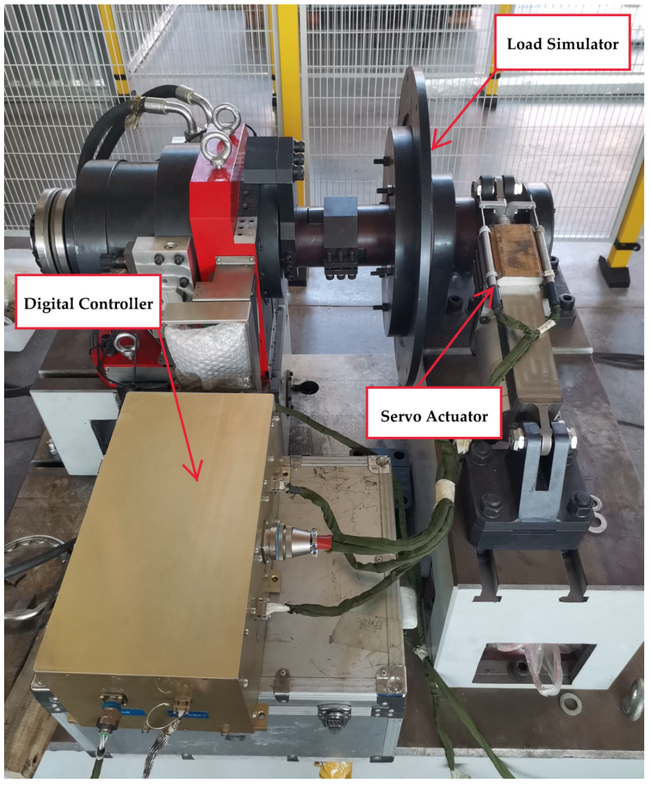
The proposed control algorithm was experimentally validated using a laboratory servo system prototype, the setup of which is illustrated in Figure 4. The experimental platform comprises a digital controller, a servo actuator, and a dynamic load simulator. The core processing unit of the digital controller is a TMS320F28335 DSP microprocessor. The system parameters are shown in

Table 1. Servo system parameters.

Parameter	Value	Parameter	Value
Nominal torque constant $K_{t0}$	0.035 N·m/A	External load torque $T_l$	≤0.8 N·m
Nominal inertia $J_0$	0.0000026 kg·m2	Temperature coefficient ${\beta }_K$	0.0012/°C
Viscous friction $B_0$	0.00025 N·m·s/rad	Temperature coefficient ${\beta }_J$	0.000024/°C
Coulomb friction $T_C$	0.02 N·m	Temperature coefficient ${\beta }_B$	0.0082/°C
Stribeck friction $T_s$	0.02 N·m	Temperature coefficient ${\beta }_{Tc}$	0.005/°C
Stribeck velocity ${\omega }_s$	1.0 rad/s	Temperature coefficient ${\beta }_{Ts}$	0.0082/°C
Velocity-dependent friction $B_v$	0.00025 N·m·s/rad	Temperature coefficient ${\beta }_{\omega s}$	0.02/°C
Transmission ratio $n$	180	Temperature coefficient ${\beta }_{Bv}$	0.0082/°C
Ambient temperature $T$	−40~280 °C

. The controller design parameters are listed in

Table 2. Controller design parameters.

Parameter	Value	Parameter	Value
FTCESO bandwidth $\rho$	150.7	Terminal exponent $q/p$	5/3
FTCESO gain $k_1$, $k_2$, $k_3$	1.5, 2.0, 2.5	Reaching law gains ${\eta }_1$, ${\eta }_2$, ${\eta }_3$	2.8, 0.55, 0.7
FTCESO exponent ${\alpha }_1$	0.75	Boundary layer $\Delta$	0.002
Slow observer bandwidth $\lambda$	0.8	Power exponent $\varsigma$	0.6
Adaptive gain $\gamma$	600	Sliding surface gain $c_1$, $c_2$, $c_3$	280, 28,000, 4.5
σ-modification σ	60

.

Based on the thermal models in Section 2.2 and the temperature coefficients in Table 1, the predicted parameter variations over the test range ΔT = 260 °C are as follows:

• Torque constant $K_t$ decreases by approximately 31.2% (Equation (3));
• Total inertia $J_{total}$ increases by approximately 0.62% (Equation (4)), which is negligible;
• Viscous damping $B$ decreases by approximately 88.1% (Equation (5));
• Coulomb friction $T_c$ increases by approximately 130% (Equation (6));
• Stribeck friction $T_s$ decreases by approximately 88.1% (Equation (6));
• Stribeck velocity ${\omega }_s$ increases by approximately 520% (Equation (6));
• Velocity-dependent friction $B_v$ decreases by approximately 88.1% (Equation (6)).

These values are model predictions based on the assumed thermal models and identified coefficients, not in situ measurements, as the actuator lacked embedded temperature sensors. Consistent with the design philosophy of the ultra-local model, all such parameter mismatches are absorbed into the lumped disturbance $F(t)$, which is estimated and compensated by the dual-layer observer without requiring real-time parameter identification.

The FTCESO switching gains $k_1$, $k_2$, and $k_3$ are selected based on the convergence conditions derived in the proof of Theorem 2. After the estimation errors enter the residual set $\Re$, exact finite-time convergence to zero requires: $k_1>{\chi }_2$ (the residual bound on $e_2$), $k_2>{\chi }_3$ (the residual bound on $e_3$), and $k_3>\overline{\xi }$ (the disturbance derivative bound in Assumption 2). For a well-tuned FTCESO with sufficiently large $\rho$, the residual $V_{res}$ is small, making ${\chi }_2$ and ${\chi }_3$ small. The values $k_1=1.5$, $k_2=2.0$, and $k_3=2.5$ satisfy these conditions with adequate margin. Their monotonically increasing pattern ($k_1<k_2<k_3$) reflects the progressively stronger correction required for higher-order estimation errors in the cascaded structure of Equation (12).

The proposed method is compared against three baseline controllers:

• PID—proportional-integral-derivative control with gain scheduling and anti-windup;
• LADRC—linear active disturbance rejection control with linear extended state observer;
• Conv. SMC—conventional sliding mode control with extended state observer.

The controller design parameters for the three baseline controllers are listed in

Table 3. Baseline controller design parameters.

Parameter	Value	Parameter	Value
PID proportional gain	30	LADRC compensation gain	78
PID integral gain	100	Conv. SMC ESO bandwidth	316 rad/s
PID derivative gain	1.5	Sliding surface coefficient	15
LADRC observer bandwidth	562 rad/s	Switching gain	20
LADRC controller bandwidth	180 rad/s	Boundary layer thickness	0.06

. All baseline controller parameters were individually tuned on the test platform. The PID gains were optimized via Ziegler–Nichols tuning, with subsequent manual refinement. LADRC observer bandwidth was selected following the standard guideline of 3–5 times the controller bandwidth. Conv. SMC ESO bandwidth was limited to 316 rad/s to avoid amplification of measurement noise in the single-layer observer structure. Each controller was tuned to achieve its best achievable performance under nominal conditions.

5.2. Experimental Results

5.2.1. Nominal Tracking Performance

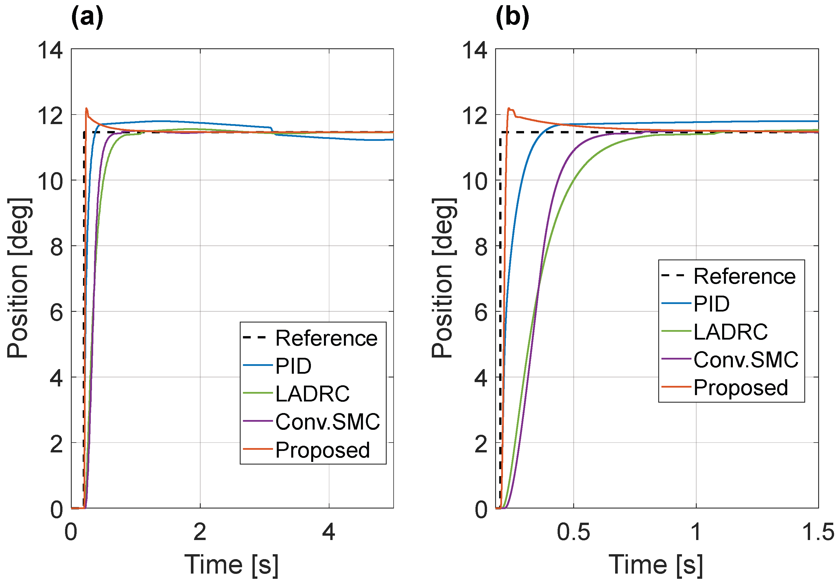
Under nominal operating conditions with constant temperature of 20 °C and absence of external disturbances, a step reference signal of 0.2 rad is applied at 0.2 s.

The tracking performance of the proposed scheme is compared with three other algorithms, as illustrated in Figure 5. Because of the finite-time convergence characteristics of both the FTCESO and the terminal sliding mode controller, the proposed method achieves the fastest transient response, with a rise time of 16 ms and an overshoot of 4.9%. In comparison, the PID controller exhibits a rise time of 92 ms and an overshoot of 4.2%. LADRC demonstrates a moderate response, characterized by a rise time of 285 ms and a notably low overshoot of 0.83%. Conventional sliding mode control (SMC) yields a rise time of 191 ms with a minimal overshoot of 0.37%. In terms of steady-state accuracy, the proposed method, along with LADRC and conventional SMC, maintains a tracking error below 0.05°. In contrast, the PID controller exhibits a comparatively larger steady-state error of approximately 0.10°.

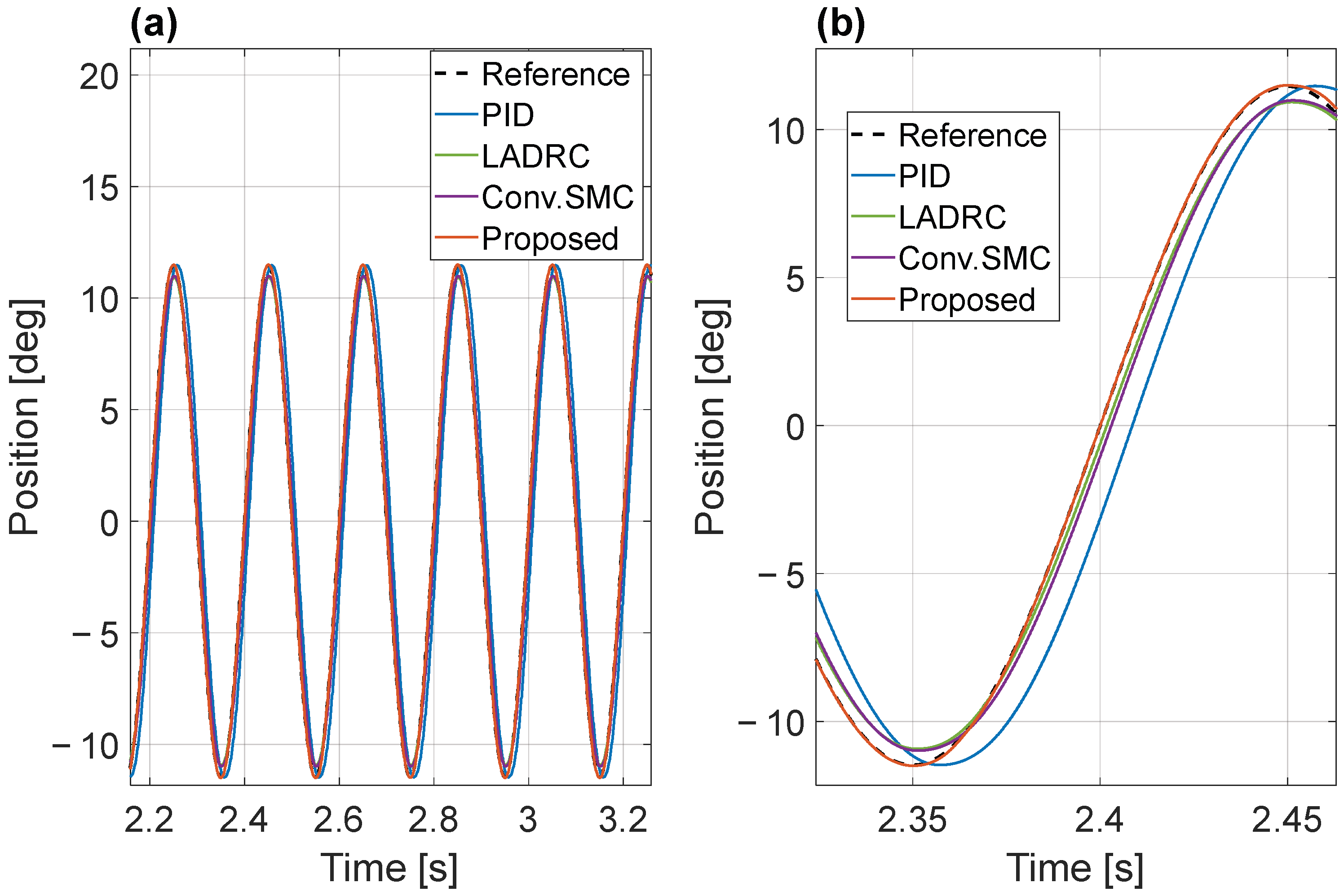
When tracking 0.2 rad amplitude, 5 Hz sinusoidal reference trajectory, the proposed method demonstrates superior tracking accuracy, maintaining a phase lag below 0.18° and an amplitude increase of 0.29%, shown in Figure 6. In comparison, the PID controller exhibits a significantly larger phase lag of approximately 15.30°, with a comparable amplitude increase of 0.20%. Both LADRC and conventional SMC offer moderate tracking performance: LADRC achieves a phase lag of about 3.24° along with an amplitude attenuation of 4.71%, while conventional SMC results in a phase lag of 5.04° and an amplitude attenuation of 4.17%. These results confirm that the proposed method provides the most effective preservation of both the phase and magnitude of the reference signal in the frequency domain.

5.2.2. High-Frequency Disturbance Rejection

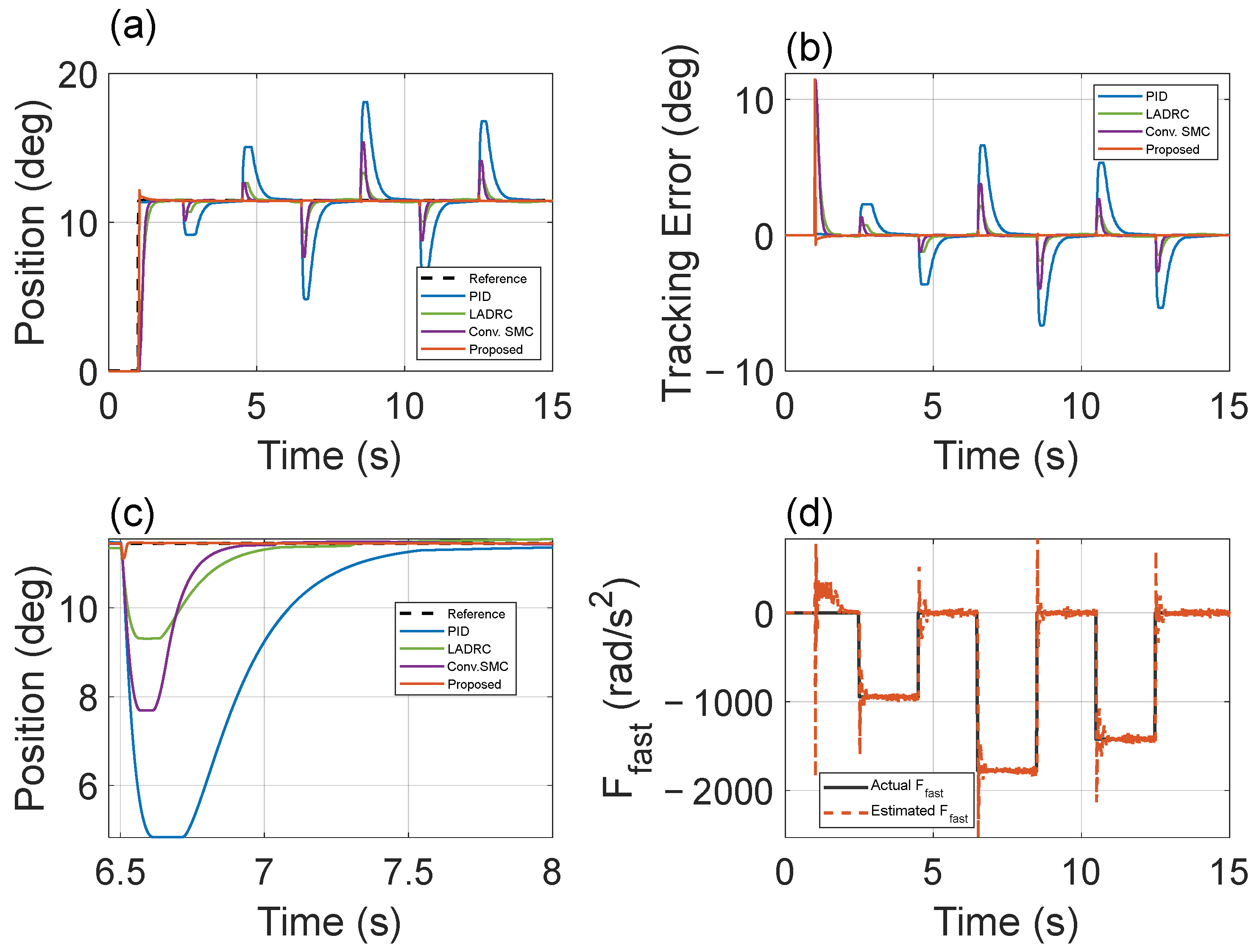
Under a step reference of 0.2 rad, step disturbance torques of 0.43 N·m, 0.80 N·m, and 0.64 N·m are sequentially applied to the servo system during the intervals t = 1.5–3.5 s, 6.5–8.5 s, and 10.5–12.5 s, respectively. The comparative results are shown in Figure 7. During the largest disturbance (0.80 N·m), the proposed method achieves the best disturbance rejection performance, with a minimum peak deviation of 0.30° and a recovery time—defined as the time required to return within a ±0.05° error band—of only 20 ms. In comparison, conventional SMC exhibits a peak deviation of 3.77° and a recovery time of 340 ms; LADRC yields a peak deviation of 2.15° with a recovery time of 488 ms; and PID control results in a peak deviation of 6.63° and requires 1140 ms to recover. The position tracking responses and error profiles clearly demonstrate the superior disturbance rejection capability of the proposed method. Figure 7d illustrates the FTCESO’s fast disturbance estimation performance, where ${\widehat{F}}_{fast}$ accurately tracks the actual injected disturbance $F_{fast}=-{\displaystyle \frac{T_l}{J_{0}n}}$ with rapid convergence.

5.2.3. Combined Severe Conditions

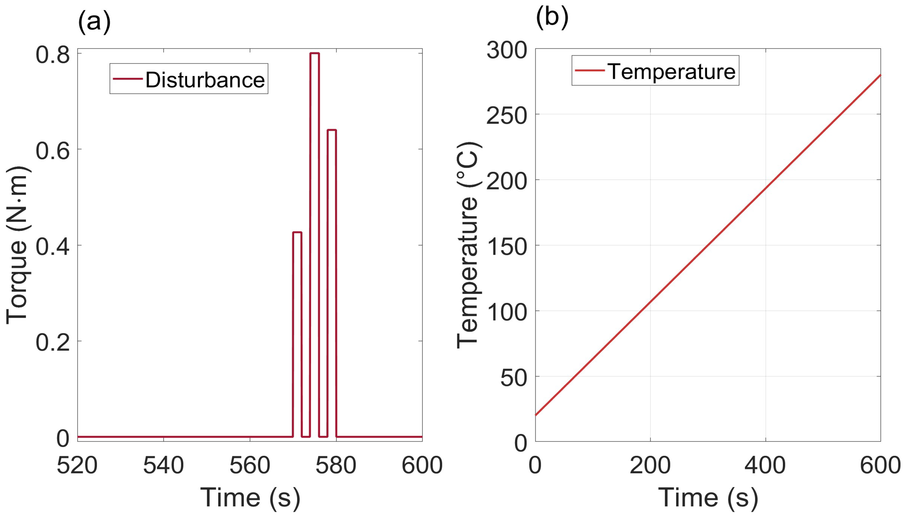
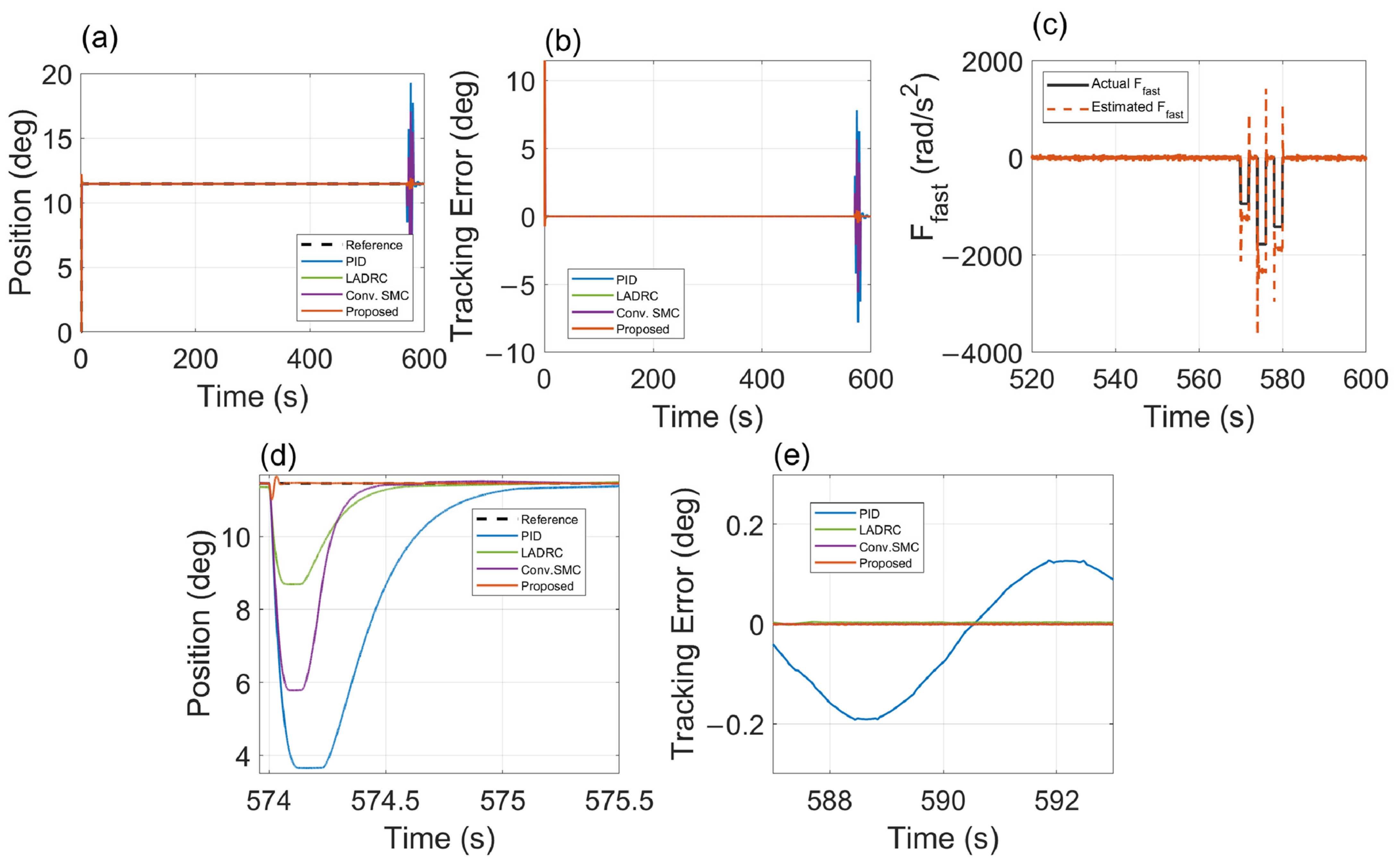
To evaluate the overall system robustness under the most demanding operational scenario—simultaneous thermal drift and high-frequency disturbances—a step reference of 0.2 rad is applied at t = 1 s, and step disturbance torques of 0.43 N·m, 0.80 N·m, and 0.64 N·m are then sequentially injected into the system during the intervals t = 570–572 s, 574–576 s and 578–580 s, respectively. Concurrently throughout the 600 s test, the ambient temperature of the servo mechanism was raised from 20 °C to 280 °C using a heating apparatus under a programmed thermal profile. The programmed temperature profile and applied load torque waveform are shown in Figure 8, and the corresponding experimental results are shown in Figure 9.

Under these combined stresses, the proposed method attains a maximum tracking error of 0.45°, occurring at t ≈ 574 s, when the largest disturbance coincides with a moderate thermal deviation. In contrast, conventional SMC yields a peak error of 5.68°, while PID and LADRC exhibit peak errors of 7.81° and 2.77°, respectively.

Following each disturbance, the proposed scheme recovers to within ±0.05° of the reference within 43 ms. By comparison, the PID controller requires 1150 ms to settle within the same bound, LADRC needs 524 ms, and conventional SMC takes 416 ms.

The proposed method, along with LADRC and conventional SMC, achieves a steady-state tracking error below 0.08°, while the PID controller exhibits a substantially larger error of approximately 0.2°.

Figure 9c demonstrates that the FTCESO accurately estimates fast disturbances $F_{fast}=-{\displaystyle \frac{T_l}{J_{0}n}}$ arising from external load torques.

The superior performance of the proposed method under such combined conditions stems from its dual-observer architecture, which independently addresses both fast and slow disturbances. Furthermore, the finite-time convergent properties of the FTCESO ensure rapid disturbance compensation, while the σ-modification adaptive law provides robustness against slow parameter drift without requiring explicit temperature measurement.

5.3. Discussion

The experimental results validate the effectiveness of the proposed dual-layer observer-based adaptive robust control strategy across three progressively challenging test scenarios. The key observations are:

• The FTCESO provides rapid and accurate estimation of fast-varying disturbances, with the finite-time convergence property ensuring predictable transient performance independent of initial conditions. As demonstrated in Figure 7d and Figure 9c, the estimated disturbance closely tracks the actual injected load disturbance.
• The slow adaptive observer effectively tracks temperature-induced parameter drifts without requiring direct temperature measurement, relying instead on the velocity estimation residual as an indirect indicator of thermal effects.
• The computational overhead is modest (400 μs per cycle on TMS320F28335), confirming suitability for embedded implementation in resource-constrained flight control systems.

It should be noted that the experimental thermal profile follows a monotonically increasing trajectory, and the external load disturbances are applied as step torques. These conditions represent a simplified abstraction of actual flight scenarios, where aerodynamic loads exhibit broadband time-varying characteristics and the thermal environment undergoes complex transient heating and cooling cycles. The step-type disturbance was adopted because it represents the worst-case scenario in terms of instantaneous disturbance magnitude, providing a stringent test of the controller’s transient rejection capability. The monotonic thermal profile was selected to systematically evaluate controller robustness across the full temperature range without introducing confounding variables from thermal cycling effects. Future work will incorporate time-varying sinusoidal and stochastic load profiles as well as mission-representative thermal trajectories derived from CFD simulations to further validate the proposed approach under more realistic conditions.

Due to the unidentified thermal dynamics of the actuator system, it remains uncertain whether the PMSM motor and mechanical components reached thermal equilibrium or what their actual temperatures were during the 600 s test duration. Future work will incorporate embedded temperature sensors to resolve this problem.

6. Conclusions and Future Work

6.1. Summary of Contributions

This paper has presented a comprehensive adaptive control strategy for PMSM-driven position servo systems operating under extreme thermal environments in high-speed flight vehicles. The key contributions and their validation are summarized as follows:

• Ultra-local model with comprehensive thermal effect integration: The ultra-local model formulation, motivated by physically consistent thermal analysis, provides a unified framework that captures temperature-dependent parameter variations without requiring real-time thermal measurements. A formal frequency-based criterion enables principled decomposition into fast and slow disturbance components.
• Dual-layer disturbance observer architecture: A systematic approach to multi-scale disturbance estimation is established through a novel two-layer observation structure, for which inter-layer stability and transient-state boundedness are rigorously proven.
• Nonlinear integral terminal sliding mode control: The controller with cycloidal reaching law achieves finite-time tracking error convergence, established via nonlinear Lyapunov analysis without linearization assumptions.
• Experimental validation: Three test scenarios demonstrate 83–94% reduction in disturbance-induced maximum position deviation and over 90% reduction in recovery time compared with PID, LADRC, and conventional SMC. Computational load analysis (400 μs per cycle) confirms real-time feasibility on the TMS320F28335 platform.

6.2. Future Work

We will focus on temperature sensing, machine learning integration, and fault-tolerant architectures.

• Temperature sensing: Deployment of distributed temperature sensor arrays within the actuator subsystem, encompassing PMSM windings and drivetrain components, to enable real-time thermal state monitoring and critical thermal zone identification.
• Machine learning integration: Development of data-driven adaptive mechanisms through the application of advanced machine learning techniques leveraging operational history data, enabling enhanced system adaptation and predictive maintenance capabilities.
• Fault-tolerant architectures: Extension of the proposed framework with redundant control pathways and real-time fault detection mechanisms to ensure reliable operation under critical failure conditions, including sensor failures and actuator degradation.

References

1. Ding, Y.; Yue, X.; Chen, G.; Si, J. Review of control and guidance technology on hypersonic vehicle. Chin. J. Aeronaut. 2022, 35, 1–18. [Google Scholar] [CrossRef]
2. Stevens, B.L.; Lewis, F.L.; Johnson, E.N. Aircraft Control and Simulation: Dynamics, Controls Design, and Autonomous Systems; John Wiley & Sons: Hoboken, NJ, USA, 2015. [Google Scholar]
3. Peters, A.B.; Zhang, D.; Chen, S.; Ott, C.; Oses, C.; Curtarolo, S.; McCue, I.; Pollock, T.M. Materials design for hypersonics. Nat. Commun. 2024, 15, 3328. [Google Scholar] [CrossRef] [PubMed]
4. Hoang, D.-T.; Nguyen, M.-D.; Kim, S.-M.; Bang, T.-K.; Kim, Y.-J.; Shin, K.-H.; Choi, J.-Y. Irreversible demagnetization prediction due to overload and high-temperature conditions in PMSM based on nonlinear analytical model. IEEE Trans. Energy Convers. 2024, 40, 2256–2267. [Google Scholar] [CrossRef]
5. Huang, K.; Ding, B.; Lai, C.; Feng, G. Flux linkage tracking-based permanent magnet temperature hybrid modeling and estimation for PMSMs with data-driven-based core loss compensation. IEEE Trans. Power Electron. 2024, 39, 1410–1421. [Google Scholar] [CrossRef]
6. Armstrong-Hélouvry, B.; Dupont, P.; de Wit, C.C. A survey of models, analysis tools and compensation methods for the control of machines with friction. Automatica 1994, 30, 1083–1138. [Google Scholar] [CrossRef]
7. de Wit, C.C.; Olsson, H.; Åström, K.J.; Lischinsky, P. A new model for control of systems with friction. IEEE Trans. Autom. Control 1995, 40, 419–425. [Google Scholar] [CrossRef]
8. Weng, L.; Gao, W.; Zhang, D.; Huang, T.; Duan, G.; Liu, T.; Shi, K. Analytical modeling of transient thermal characteristics of precision machine tools and real-time active thermal control method. Int. J. Mach. Tools Manuf. 2023, 186, 104003. [Google Scholar] [CrossRef]
9. Wang, M.; Lu, W.; Zhang, K.; Zhu, X.; Wang, M.; Yang, B.; Gao, X. Thermal error prediction of ball screws in full-time series using working condition data based on a mechanism and data hybrid-driven model. Int. J. Adv. Manuf. Technol. 2024, 133, 1443–1462. [Google Scholar] [CrossRef]
10. Li, C.; Xu, M.; Song, W.; Zhang, H. A review of static and dynamic analysis of ball screw feed drives, recirculating linear guideway, and ball screw. Int. J. Mach. Tools Manuf. 2023, 188, 104021. [Google Scholar] [CrossRef]
11. Gao, X.; Zhang, K.; Zhang, Z.; Wang, M.; Zan, T.; Gao, P. XGBoost-based thermal error prediction and compensation of ball screws. Proc. Inst. Mech. Eng. Part B J. Eng. Manuf. 2024, 238, 151–163. [Google Scholar] [CrossRef]
12. Hou, Q.; Zuo, Y.; Sun, J.; Lee, C.H.T.; Wang, Y.; Ding, S. Modified nonlinear active disturbance rejection control for PMSM speed regulation with frequency domain analysis. IEEE Trans. Power Electron. 2023, 38, 8126–8134. [Google Scholar] [CrossRef]
13. Zhao, C.; Guo, L. Towards a theoretical foundation of PID control for uncertain nonlinear systems. Automatica 2022, 142, 110360. [Google Scholar] [CrossRef]
14. Campos, V.C.S.; Nguyen, A.-T.; Palhares, R.M. Adaptive gain-scheduling control for continuous-time systems with polytopic uncertainties: An LMI-based approach. Automatica 2021, 132, 109856. [Google Scholar]
15. Zhang, S.; Shen, A.; Luo, X.; Tang, Q.; Li, Z. Multi-sliding mode current disturbance suppression scheme based model reference adaptive system for sensorless control of permanent magnet synchronous motor. ISA Trans. 2023, 137, 615–628. [Google Scholar] [CrossRef]
16. Gabbi, T.S.; de Araujo, M.B.; Rocha, L.R.; Scalcon, F.P.; Gründling, H.A.; Vieira, R.P. Discrete-time sliding mode controller based on backstepping disturbance compensation for robust current control of PMSM drives. ISA Trans. 2022, 128, 581–592. [Google Scholar] [CrossRef]
17. Guo, X.; Huang, S.; Lu, K.; Peng, Y.; Wang, H.; Yang, J. A fast sliding mode speed controller for PMSM based on new compound reaching law with improved sliding mode observer. IEEE Trans. Transp. Electrif. 2023, 9, 2955–2968. [Google Scholar] [CrossRef]
18. Ma, L.; Mei, K.; Ding, S.; Pan, T. Design of adaptive fuzzy fixed-time HOSM controller subject to asymmetric output constraints. IEEE Trans. Fuzzy Syst. 2023, 31, 2989–2999. [Google Scholar] [CrossRef]
19. Levant, A. Quasi-continuous high-order sliding-mode controllers. IEEE Trans. Autom. Control 2005, 50, 1812–1816. [Google Scholar] [CrossRef]
20. Shi, S.; Dai, L.; Min, H.; Yang, J.; Li, S. Prescribed-time nonsingular terminal sliding mode control and its application in PMSM servo systems. IEEE Trans. Ind. Electron. 2025, 72, 1734–1743. [Google Scholar] [CrossRef]
21. Han, J. From PID to active disturbance rejection control. IEEE Trans. Ind. Electron. 2009, 56, 900–906. [Google Scholar] [CrossRef]
22. Razmjooei, H.; Palli, G.; Janabi-Sharifi, F.; Alirezaee, S. Adaptive fast-finite-time extended state observer design for uncertain electro-hydraulic systems. Eur. J. Control 2023, 69, 100749. [Google Scholar] [CrossRef]
23. Benyahia, A.; Stanković, M.; Madonski, R.; Babayomi, O.; Manojlović, S. Improving control performance by cascading observers: Case of ADRC with cascade ESO. IEEE/CAA J. Autom. Sin. 2025, 12, 1702–1712. [Google Scholar] [CrossRef]
24. Fliess, M.; Join, C. Model-free control. Int. J. Control. 2013, 86, 2228–2252. [Google Scholar] [CrossRef]
25. Jia, T.; Liu, J.; Wang, Y.; Li, C.; Zhang, H. An improved LuGre friction model and its parameter identification of structural interface in thermal environment. Mech. Syst. Signal Process. 2024, 216, 111468. [Google Scholar] [CrossRef]
26. Yang, Y.; Li, L.; Zhang, H. Thermal demagnetization characteristics of NdFeB used in eddy current dampers. IEEE Access 2024, 12, 71304–71322. [Google Scholar] [CrossRef]
27. Callister, W.D., Jr.; Rethwisch, D.G. Materials Science and Engineering, 10th ed.; Wiley: Hoboken, NJ, USA, 2018. [Google Scholar]
28. Xiao, B.; Huang, J.; Tang, D.; Xu, Z. Dynamic modeling of the electrical actuation system of the hypersonic aircraft considering the temperature effects. Aerosp. Syst. 2024, 7, 385–393. [Google Scholar] [CrossRef]
29. Qiu, Y.; Zhou, C.; Ou, Y.; Feng, F. Theoretical and experimental analysis of the temperature rise of a ball screw. Int. J. Adv. Manuf. Technol. 2023, 127, 4455–4467. [Google Scholar] [CrossRef]
30. Bhat, S.P.; Bernstein, D.S. Finite-time stability of continuous autonomous systems. SIAM J. Control Optim. 2000, 38, 751–766. [Google Scholar] [CrossRef]
31. Bhat, S.P.; Bernstein, D.S. Geometric homogeneity with applications to finite-time stability. Math. Control Signals Syst. 2005, 17, 101–127. [Google Scholar] [CrossRef]
32. Zimenko, K.; Polyakov, A.; Efimov, D.; Kremlev, A. Homogeneity based finite/fixed-time observers for linear MIMO systems. Int. J. Robust Nonlinear Control 2023, 33, 8870–8889. [Google Scholar] [CrossRef]
33. Ioannou, P.A.; Kokotovic, P.V. Instability analysis and improvement of robustness of adaptive control. Automatica 1984, 20, 583–594. [Google Scholar] [CrossRef]
Figure 1. Schematic of the PMSM-driven position servo system.
Electronics 15 01742 g001
Figure 2. Dual-layer observer architecture.
Electronics 15 01742 g002
Figure 3. Complete control system block diagram.
Electronics 15 01742 g003
Figure 4. The experimental platform.
Electronics 15 01742 g004
Figure 5. Nominal tracking performance comparison for step response. (a) Step response; (b) step response detail (0.1–1.5 s).
Electronics 15 01742 g005
Figure 6. Nominal tracking performance comparison for sine response. (a) Sine response; (b) sinusoidal tracking detail (2.32.50 s).
Electronics 15 01742 g006
Figure 7. High-frequency disturbance rejection performance. (a) Position tracking under step disturbances; (b) tracking error comparison; (c) position tracking detail (6.4–8 s); (d) FTCESO disturbance estimation for proposed method.
Electronics 15 01742 g007
Figure 8. Combined severe conditions. (a) Applied load torque waveform (520–600 s); (b) programmed temperature profile.
Electronics 15 01742 g008
Figure 9. Combined severe conditions performance. (a) Position tracking under thermal drift and disturbance loading; (b) tracking error comparison; (c) FTCESO disturbance estimation for proposed method; (d) position tracking detail during disturbance events (573.8–574.3 s); (e) tracking error detail during no disturbance events (587–593 s).
Electronics 15 01742 g009