Article

Combining Interpolation Techniques and Lightweight Convolutional Neural Networks for Partial Discharge Image Signal Identification in Transformer Bushings


Department of Computer Science and Information Engineering, Ming Chuan University, Taoyuan Campus, Guishan District, Taoyuan City 333, Taiwan
Electronics 2026, 15(8), 1584; https://doi.org/10.3390/electronics15081584
Submission received: 20 March 2026 / Revised: 4 April 2026 / Accepted: 8 April 2026 / Published: 10 April 2026

Abstract

Partial discharge detection is a key technology for maintaining the normal operation of industrial power equipment. Oil-impregnated paper bushings are crucial components connecting transformers to the power grid. Insulation degradation leads to partial discharge, posing a significant threat to power system operation. Developing on-line diagnostics for partial discharge in transformer bushings and automatic identification of insulation defects can effectively protect system and personnel safety. Due to limitations of small sample sizes and lightweight networks, this study combines interpolation techniques with a lightweight convolutional neural network to improve identification accuracy. This network uses interpolation to maintain the undistorted sample signal from the initial input and reduces training defects from a small sample size. The neural network extracts partial discharge features to determine the defect type and its cause. This study uses a publicly available dataset with discharge signals from generators. Although from a different source from the discharge signals generated by oil-impregnated paper bushings, the signal distribution is similar, allowing for a fair analysis and providing a reference for evaluating discharge signals obtained from oil-impregnated paper bushings or other discharge devices. The experimental results show that the accuracy of this network improved from 97% to over 99% while maintaining low computational complexity and excellent real-time performance. Furthermore, this network was implemented and validated on existing industrial equipment.

1. Introduction

With the rise of artificial intelligence, stable power is the most important key factor in maintaining high-efficiency artificial intelligence results. Due to the influence of environmental factors such as electric field strength, temperature, humidity and other operating factors, the insulation system of primary equipment will deteriorate over time. How to predict this in advance is a topic of interest for all researchers and engineers. No system prediction or simulation can compare to the accuracy of timely detection of signals by sensors. Among them, partial discharge (PD) measurement is an efficient and highly sensitive method, but it requires high-level operational skills in data collection, processing and analysis [1,2]. The main reason is that in current industrial equipment, there is a lack of readily available sensors for installation and convenient fields for PD signal acquisition. Therefore, it is not easy to obtain a small amount of PD signals, and it is even more difficult to use neural networks that require a large amount of data for training. Oil-impregnated paper bushings are key components that are widely used in the outgoing lines and through-wall leads of power transformers. In power systems with voltage levels higher than 110 kV, oil-impregnated paper bushings are the main type of high-voltage bushings, with a usage rate of up to 93% [3].
In actual operation, these slender bushings must withstand high voltages, high currents and strong mechanical loads for a long time and are also affected by environmental factors such as internal and external temperature changes, rain, fog and pollution. Compared with other transmission lines and internal components, their insulation performance must be subjected to more severe tests. The insulation degradation of oil-impregnated paper bushings can lead to partial discharge, which poses a major threat to the safe operation of the power system, such as voltage instability or short circuits, and may also endanger other systems [4]. Different types of partial discharge reflect different insulation degradation mechanisms and the degree of damage to the insulation capacity of the equipment. Partial discharge signal identification mainly includes time-resolved partial discharge (TRPD) mode and phase-resolved partial discharge (PRPD) mode. The PRPD mode has the advantages of mature technology, good stability and low data requirements, and is widely used. It is a reference for the first step for researchers and industries to introduce PD detection function. Currently, the identification of partial discharge defect types mainly uses statistical algorithms for feature extraction [4,5,6], which relies on human experience and has certain limitations when classifying the partial discharge signals of oil-impregnated paper sleeves. Just like in image processing technology, a corresponding classifier needs to be designed for feature extraction. Furthermore, because the partial discharge signals of oil-impregnated paper sleeves have strong randomness, the traditional human experience method is bound to have certain instability [7].
In recent years, the ability of deep learning methods to adaptively extract data features has been widely recognized in academia and industry. Deep learning-based classification algorithms, such as deep neural networks and convolutional neural networks (CNNs), have been increasingly applied to the field of partial discharge pattern recognition [8,9]. However, deep learning requires a large number of different types of fault samples for training to achieve higher classification accuracy [10,11,12]. Discharge phenomena based on insulation degradation are low-probability events, resulting in insufficient fault samples, which poses a significant challenge to neural networks that require extensive data for training. Even with the design and construction of experimental platforms, it is difficult to obtain tens of thousands of partial discharge samples through manual experiments. Even with artificial simulation, it is extremely difficult to control in demanding power field environments. When samples are insufficient, complex deep feature extraction networks are prone to overfitting during training. Although researchers have proposed many lightweight neural network architectures in recent years, they mainly focused on the compression and optimization of large networks, and the network size remains relatively large. Although a research team designed a micro-convolutional neural network [13] structure based on small samples, which not only achieved higher classification accuracy but also showed strong real-time performance, the input data still needed to be reduced to a 28 × 28 resolution, and the accuracy could only be maintained at around 97%. In addition, the feasibility of this technology in practical industrial applications with limited hardware resources has not been explored.

2. Materials and Methods

To improve recognition accuracy and maintain a lightweight neural network model, this study proposes integrating an interpolation algorithm into the neural network. The following will introduce the interpolation algorithm and the integrated model.

Introduction to the Lanczos Interpolation Algorithm

Lanczos resampling is an advanced interpolation method used for digital signal processing, particularly for scaling images and other sampled data. It uses a truncated windowed sinc function as its kernel function to approximate an ideal low-pass filter, as shown in (1), thereby reconstructing a band-limited signal from discrete samples. This method effectively interpolates new pixel values by convolving the input signal with a Lanczos kernel while maintaining sharpness and minimizing aliasing, which is the most important concern in signal processing and the main factor affecting signal distortion [14]. After multiple experimental verifications, it has become the standard choice in graphics software and image processing workflows.
L x = s i n c x s i n c x a , i f a < x < a 0 , o t h e r w i s e
The core of Lanczos resampling lies in its kernel function, which is usually defined by parameter a (usually 2 or 3, which determines the width of the kernel). Windowing is achieved through a second sinc function, which limits the kernel to 2 × a neighboring sample. This method reduces ringing artifacts compared to unwindowed sinc interpolation while maintaining a better frequency response than polynomial-based methods such as Bicubic interpolation. For down-sampling, it acts as an anti-aliasing filter by attenuating frequencies higher than the new sampling rate. Since parameter a = 3 can better preserve details, it is usually preferred for photographic images, but larger values increase computation and may cause edge overshoot [14]. In practical applications, as shown in (2), taking a one-dimensional signal as an example, if the input signal is Si, where i is an integer value, then the output S(x) can be obtained by performing discrete convolution of Si with a Lanczos kernel.
S x = i = x a + 1 x + a s i L ( x i )
Despite the numerous advantages of Lanczos resampling, the oscillating nature of the sinc function can introduce slight overshoot and halos around sharp transition areas. This may require post-processing cropping in some applications. However, for PD signals, the need for visual detail is less critical than in image processing; maintaining signal consistency without distortion is sufficient. Therefore, overall, because Lanczos is based on Fourier analysis and has demonstrated excellent empirical performance in maintaining perceived image quality, it remains the benchmark for resampling quality.
A partial discharge architecture based on Lanczos interpolation and a lightweight CNN is proposed.
While CNNs extract intrinsic features from images using continuously learned convolutional kernels, they can achieve adaptive feature extraction without the need for manual statistical extraction. In addition, their performance far surpasses previously used and effective neural networks that use manually designed features, such as AlexNet, VGG, and ResNet, which rely on a small number of samples to identify partial discharge spectral patterns in bushing. This strategy is not only time-consuming, but it is also prone to overfitting due to the small sample size.
In the past, MNIST successfully applied the first generation of artificial intelligence to handwriting recognition neural networks using a small amount of data and a lightweight network design. Therefore, in order to reduce the complexity of CNNs and meet the requirements of a small sample size, a lightweight CNN was proposed [13]. Its implementation results are satisfactory, and it is believed that it can be ported to practical embedded systems. However, there are still two problems with this architecture: First, directly reducing the input resolution to 28 × 28 only achieves a recognition result of 97%, and additional methods are needed to further improve the accuracy to meet the high precision requirements of industry. Second, existing embedded systems with ADCs and DACs are needed to simulate and verify the sensor measurement results to ensure its feasibility.
Therefore, this study proposes an integrated interpolation algorithm and lightweight CNN method based on reference [13] and ported it to an embedded system. The overall system schematic is shown in Figure 1. First, at the input end, the input image is processed through the interpolation algorithm, and the 28 × 28 output is used as the subsequent lightweight convolutional neural network for training and recognition applications. This study implemented this CNN on an embedded system platform with ADC input, used the existing DAC connected to the embedded system to simulate the sensor output, and used the ADC to identify the measurement results on the embedded system.

3. Results

3.1. Partial Discharge Dataset Description

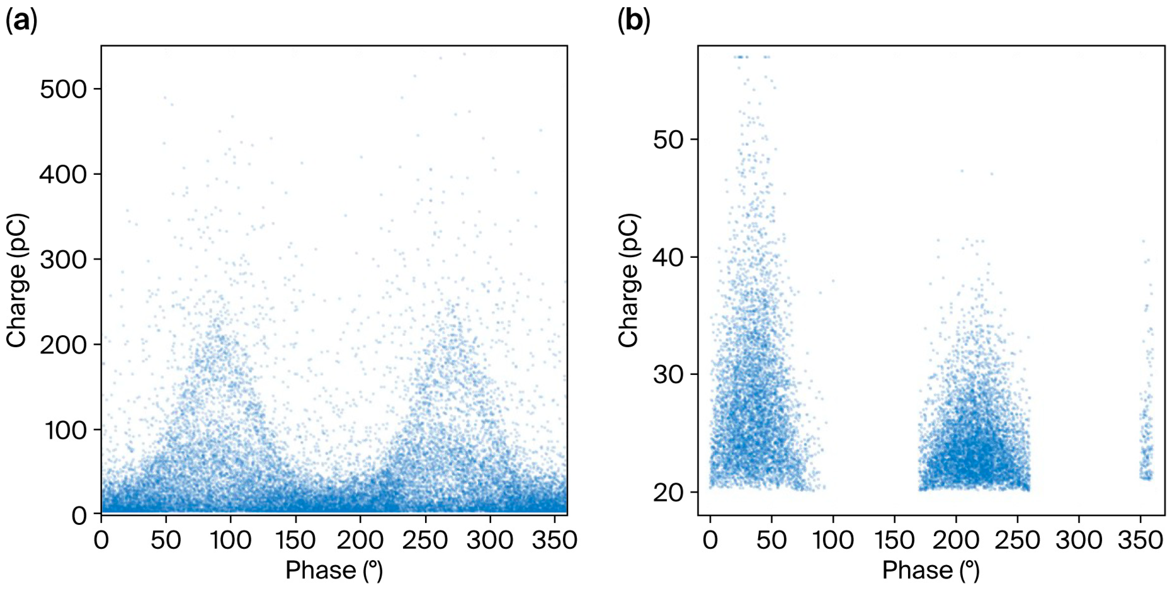
The transformer bushing PRPD signals from Ref. [13] and our simulation diagram are shown in Figure 2. However, obtaining the actual data is difficult, and there are also restrictions on obtaining it due to privacy rights. In comparison, analytical images of generator partial discharge phase mode are easier to obtain. In terms of signal distribution, the signal modes are similar, that is, the distributions of discharge signals with different phases and periods are similar. Therefore, the publicly available dataset of generator partial discharge phase modes [15] was used for simulation analysis.
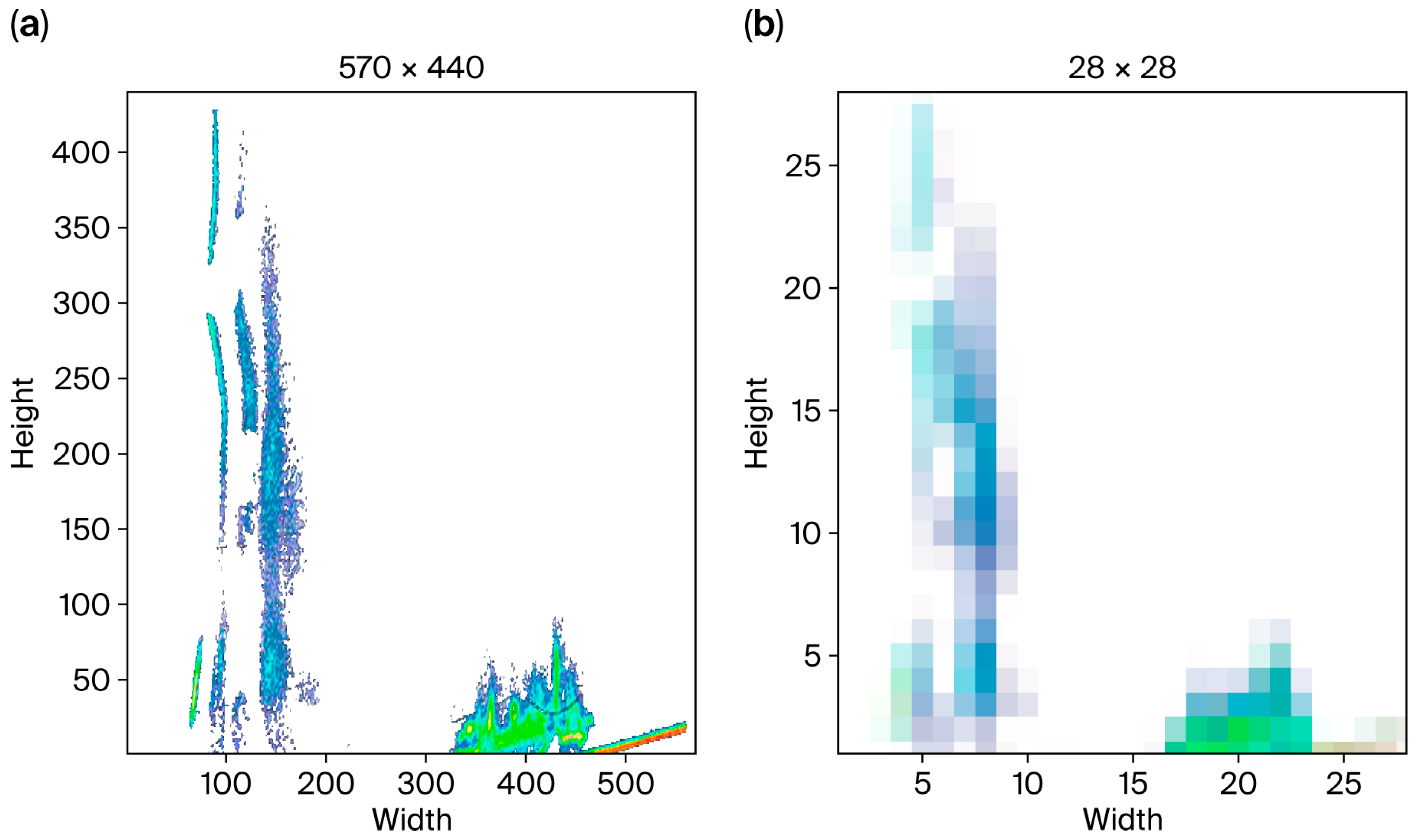
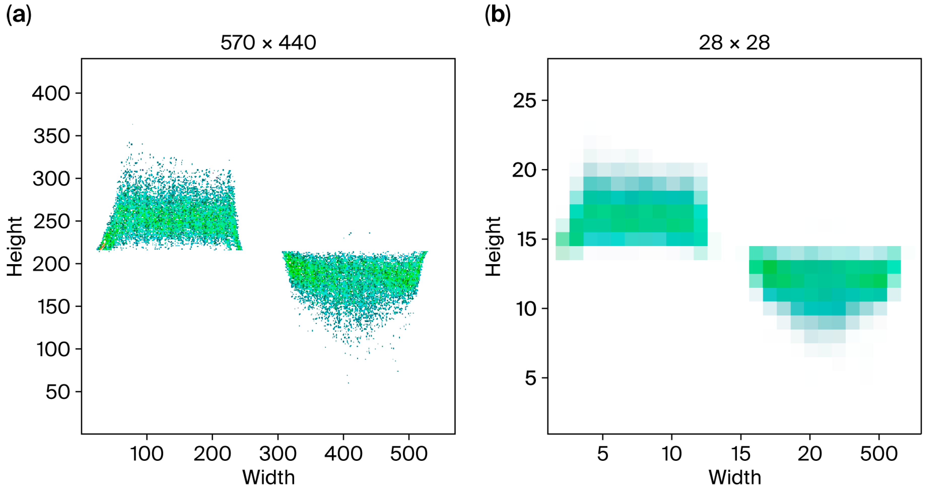
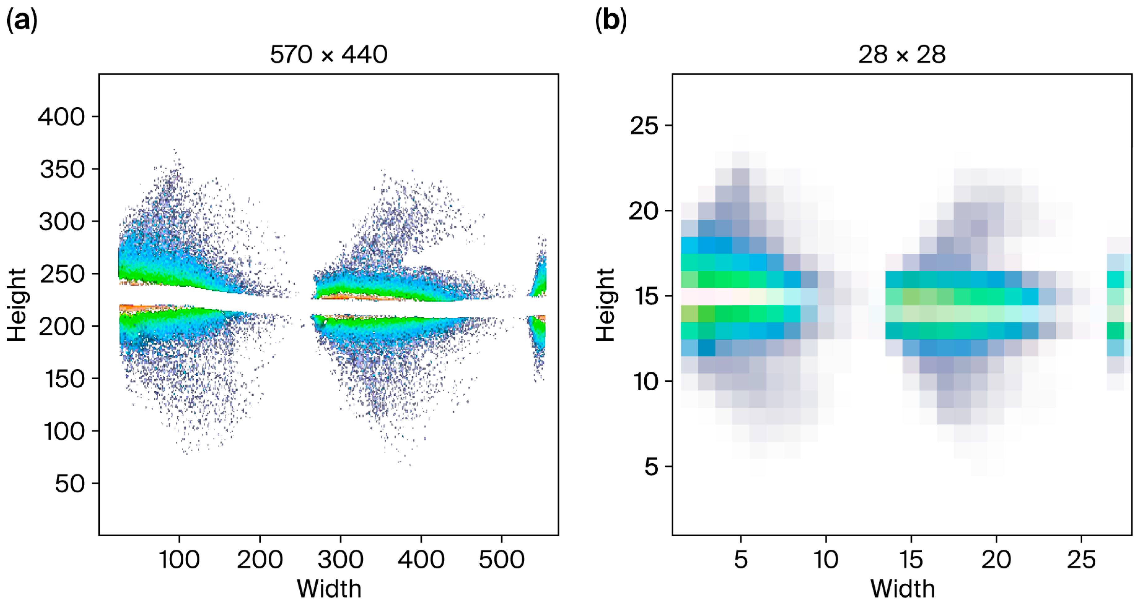
Through clustering statistics, the PRPD spectra of insulation defects were divided into three categories [15]: corona (616 images), internal (609 images), and surface (632 images). A total of 1857 PRPD spectra were obtained using this method. Figure 3, Figure 4 and Figure 5 show the resolution of the original input data and the resolution of the modified input data for different PD types. The input specification of analog-to-digital converters (ADCs) commonly used in existing industrial hardware is 50 M bits per second; therefore, 28 × 28 resolution images can be matched with existing hardware devices. To verify the network’s performance, 70% of the PRPD spectrum was randomly selected as the training set, and the remaining 30% as the test set. The dataset comprises a validation set and a test set, each accounting for 15%. Table 1 lists the sample size for the different types of discharge signals used for training, validation, and testing.

3.2. Data Simulation Analysis

For each piece of data used in training or testing, it was pre-processed using the Lanczos interpolation algorithm to convert it into 28 × 28 values. Regarding experimental parameter configuration, this study set the batch size to 4, the number of iterations to 500, the learning rate to 0.0001, the optimization rate to Adam, and used rules as the active function.
While accuracy is a commonly used metric in general applications, it is not the best tool for evaluating patterns because false positives are not included in the overall performance assessment. Therefore, recall should also be considered, especially in datasets with imbalanced sample distributions between categories. For defect detection applications, error tolerance becomes exceptionally important, and higher recall is even more crucial. Furthermore, to add a more comprehensive evaluation method, the F1 score is another effective reference metric. The F1 score can help us find the optimal balance between accuracy and recall. Regarding the subsequent data presentation, this study used accuracy, precision, recall, and F1 score to evaluate pattern performance. Table 2 lists the precision, recall, and F1 score for each defect category. These results are from one of ten random sampling training sessions. Since the results were nearly identical each time, only one set of results is presented.
Previous research [13] showed that directly sampling the raw input to 28 × 28 pixels without any compensation could achieve an average accuracy of approximately 97%, as shown in Table 2. This study proposes using the Lanczos interpolation algorithm to compensate for signal distortion during down sampling, thereby enhancing the effect of input correction to 28 × 28 pixels, thus improving the efficiency achieved by previous studies and bringing it closer to practical applications. Therefore, this study extends this advantage. At the same learning rate of 0.0001, the overall accuracy, precision of various defects, recall, and F1 score all exceeded 99%, meeting the performance requirements for partial discharge defect detection.
To more broadly compare the effects of different interpolation techniques on this neural network and explain why the Lanczos interpolation algorithm was chosen, this study also simulated the results of three other common and important interpolation algorithms using this neural network, namely Bilinear, Bicubic and B-Spline, as shown in Table 2. The data shows that Bilinear and Bicubic can achieve an average accuracy of about 98%, while B-Spline only achieves 97%. Compared with Lanczos, which was used in this study, there is a 1% difference. In terms of theoretical analysis, Bilinear and Bicubic use the values of the surrounding neighbors as compensation, which proportionally shrinks PD signals. However, compared with B-Spline, due to the large reduction ratio, the advantage of using multiple references compensates for prediction inaccuracy, which makes the results not as good as the neighbor shrinking method used in the original paper [13].
Among the accuracy metrics, Precision, Recall, and F1 score can reflect the overall performance of this neural network, but they cannot reflect its potential shortcomings or limitations in use. To further analyze this algorithm, this study used a confusion matrix to analyze this neural network’s misclassification of different signal samples. Table 3 lists four different interpolation methods, namely Nearest Neighbor, Bilinear, Bicubic, B-Spline, and Lanczos. Combined with the neural network [13], confusion matrix analysis was performed for three PD signals: corona, internal, and surface. The Lanczos interpolation method only misclassified internal and surface signals, while the other three interpolation methods misclassified two sets of signals. Further analysis of the reason for the misclassification of the Lanczos interpolation method reveals that when internal and surface signals are reduced to a low resolution of 28 × 28, their distributions are indeed similar, which can be observed visually from Figure 4b. For the remaining signal confusion comparisons, the Lanczos interpolation method performed better than the other interpolation methods.

3.3. Implementing Neural Networks in Embedded Systems with ADCs and DACs

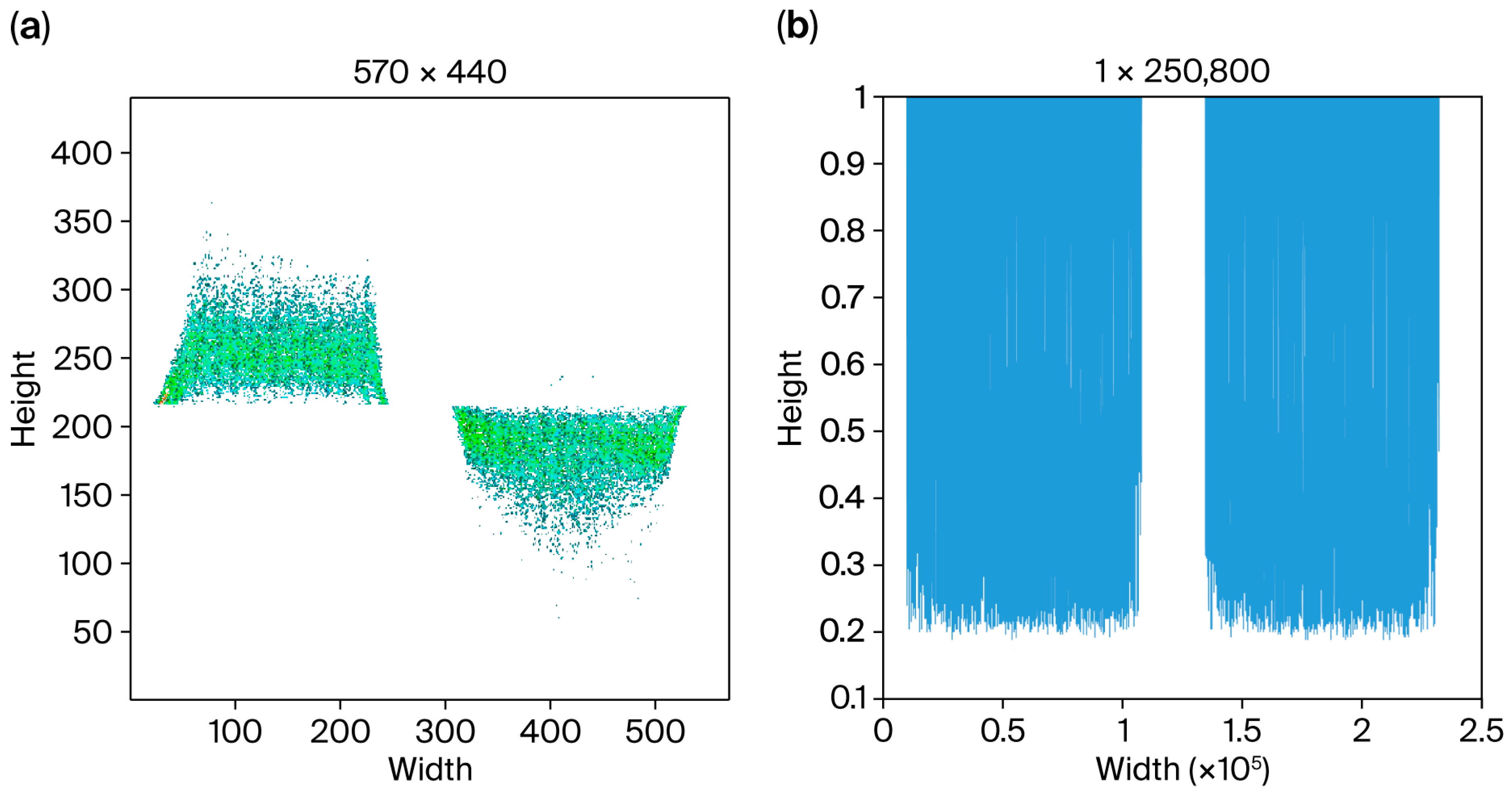
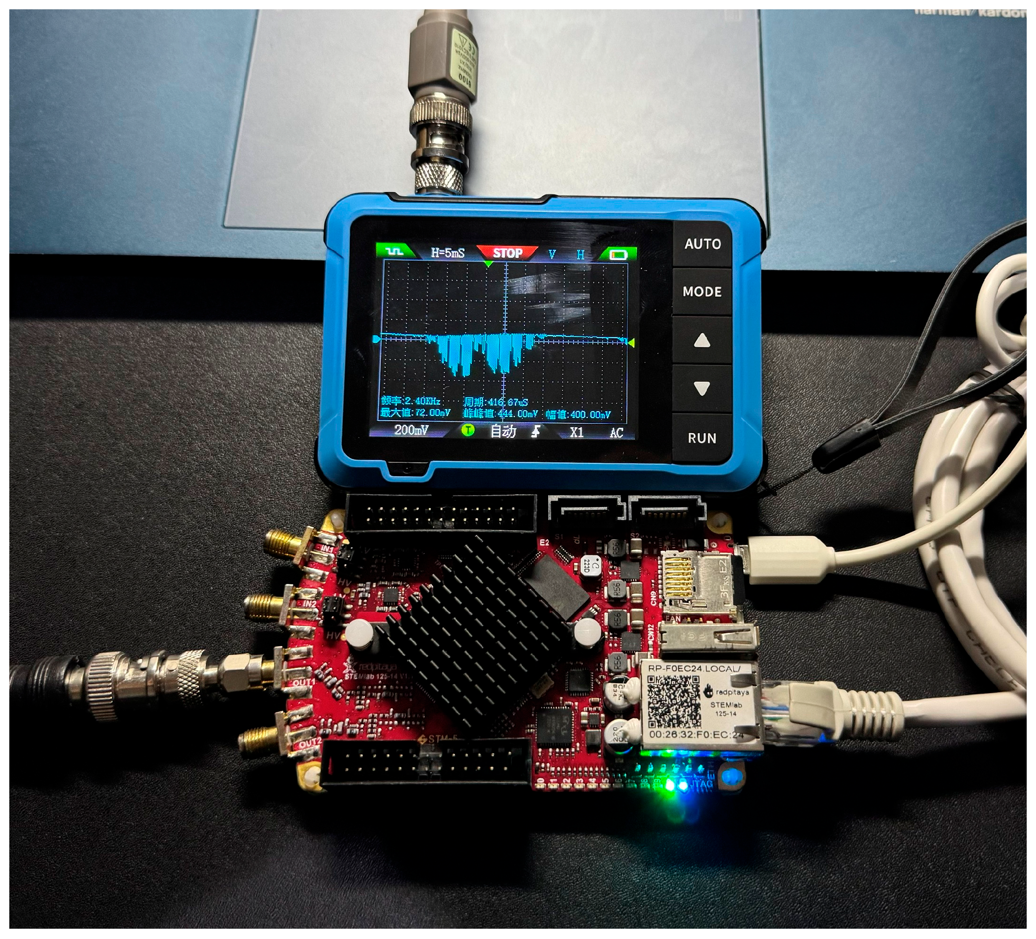
In the laboratory testing, we used an embedded system [16] to convert three different partial discharge signals using a digital-to-analog converter (DAC) and observed these signals on an oscilloscope to verify their consistency with the simulation results, which confirmed that the subsequent testing equipment could obtain accurate data. The Zynq 7000 SoC host device is equipped with a dual-core Arm Cortex-A9 processor clocked at 866 MHz with 1 GB of RAM. For example, we converted the image from 570 × 440 pixels to 1 × (570 × 440) pixels and used the DAC configured in the embedded system as its output to simulate the sensor measurement results, as shown in Figure 6 and Figure 7. In this way, we can simulate the signals actually measured by the sensor based on different databases, making it closer to a real environment. After the signal generation verification is completed using the DAC, the signal reception can be performed using the ADC, and the proposed neural network algorithm can be used for discharge identification. To achieve a broader comparison, three common lightweight neural networks—ShuffleNetV2, MobileNetV2, and ResNet-18—were also tested in combination with different interpolation algorithms. Table 4 shows the computation time required for the different interpolation algorithms combined with a neural network that were executed on an embedded system. While the other three neural networks also possess lightweight characteristics, they still require more network layers compared to the proposed network. In terms of time, the network proposed in this study can complete the inference of a single image in just 49.67 ms, of which, the neural network takes 34 ms and the interpolation algorithm takes 15 ms. Even MobileNetV2 still required 54.55 ms of computation time. Therefore, the results indicate that it is the fastest network among all currently existing lightweight networks. The actual neural network computation time is listed in Table 4. The ADC runs at 48 Mbps, and the number of frames per second can be estimated based on the input sample data. According to the resolution of 570 × 440 bytes proposed in [15], 48,000,000/(570 × 440 × 8) = 24 fps. The number of parameters and amount of memory needed for the different models are listed in Table 5.
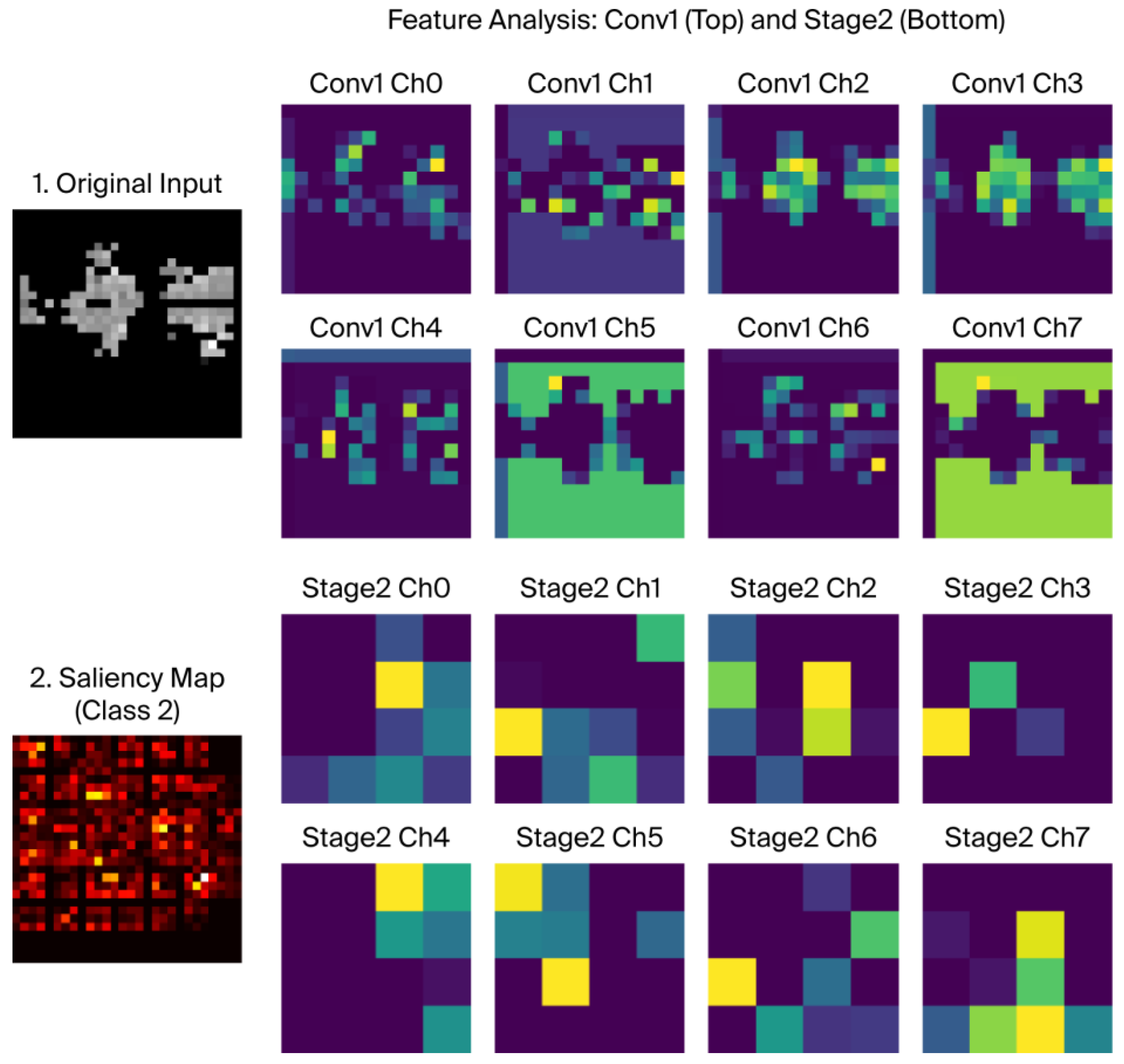
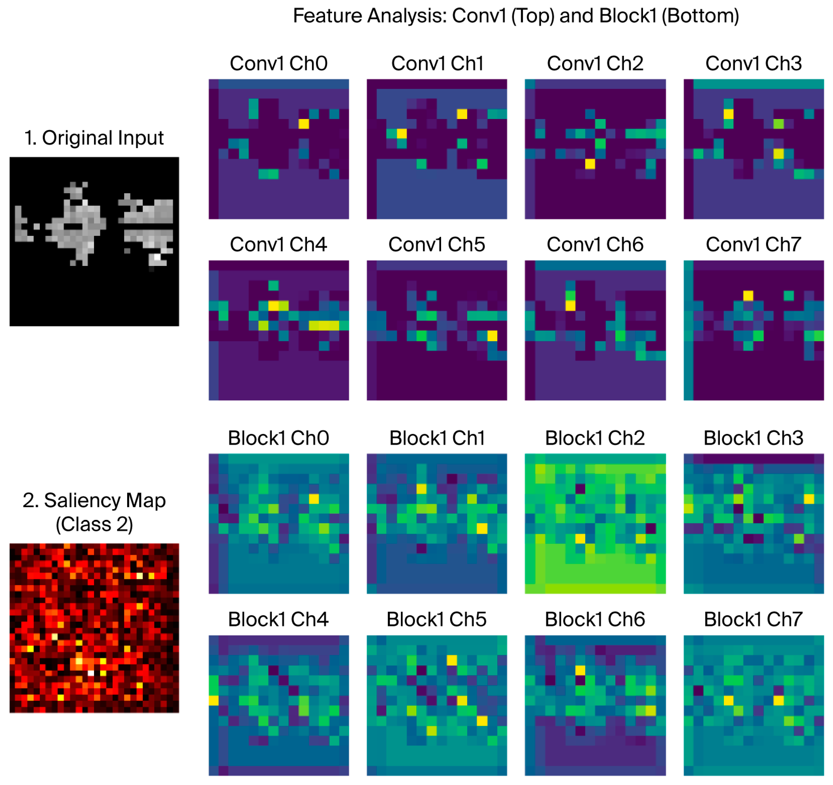
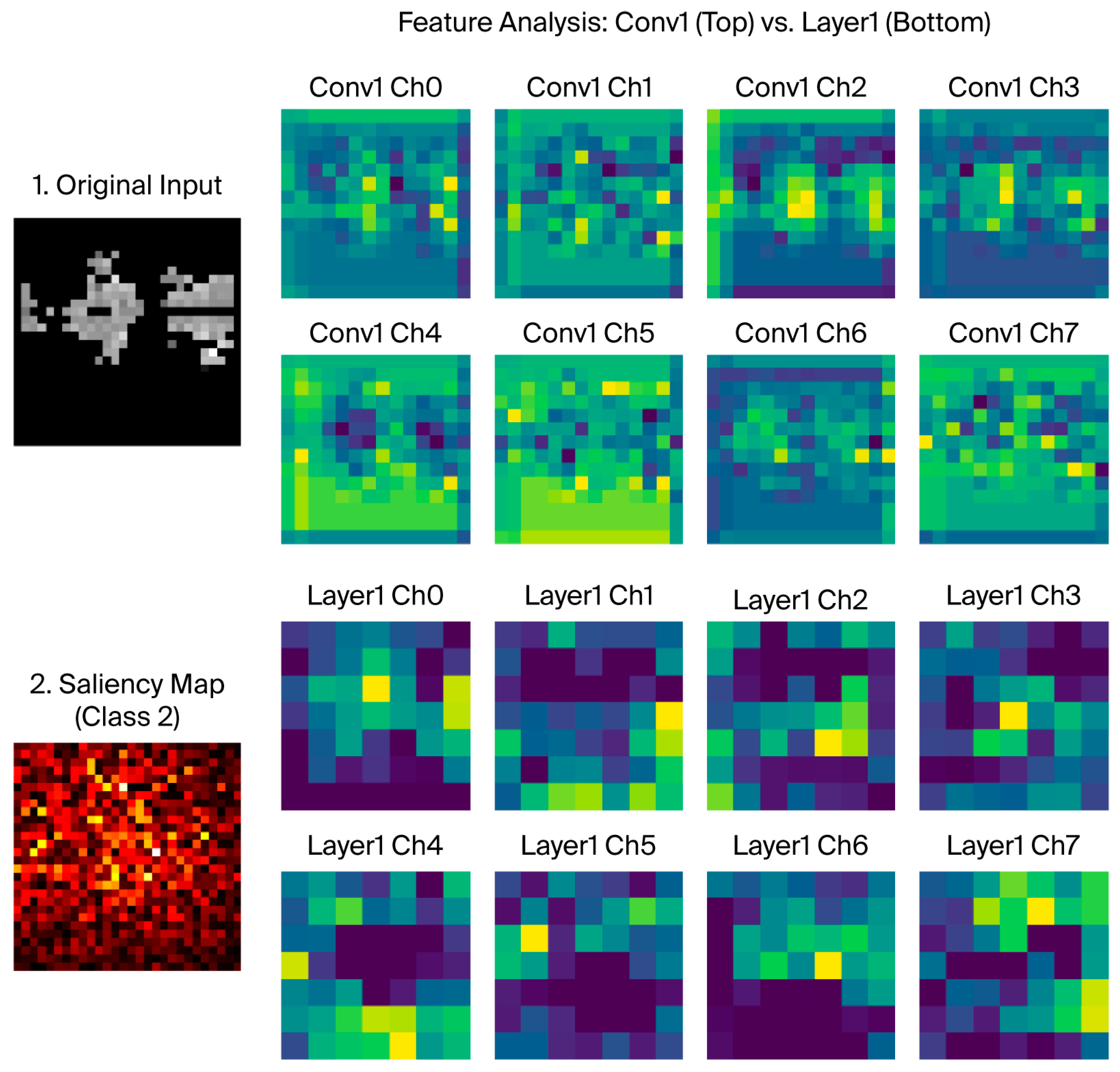
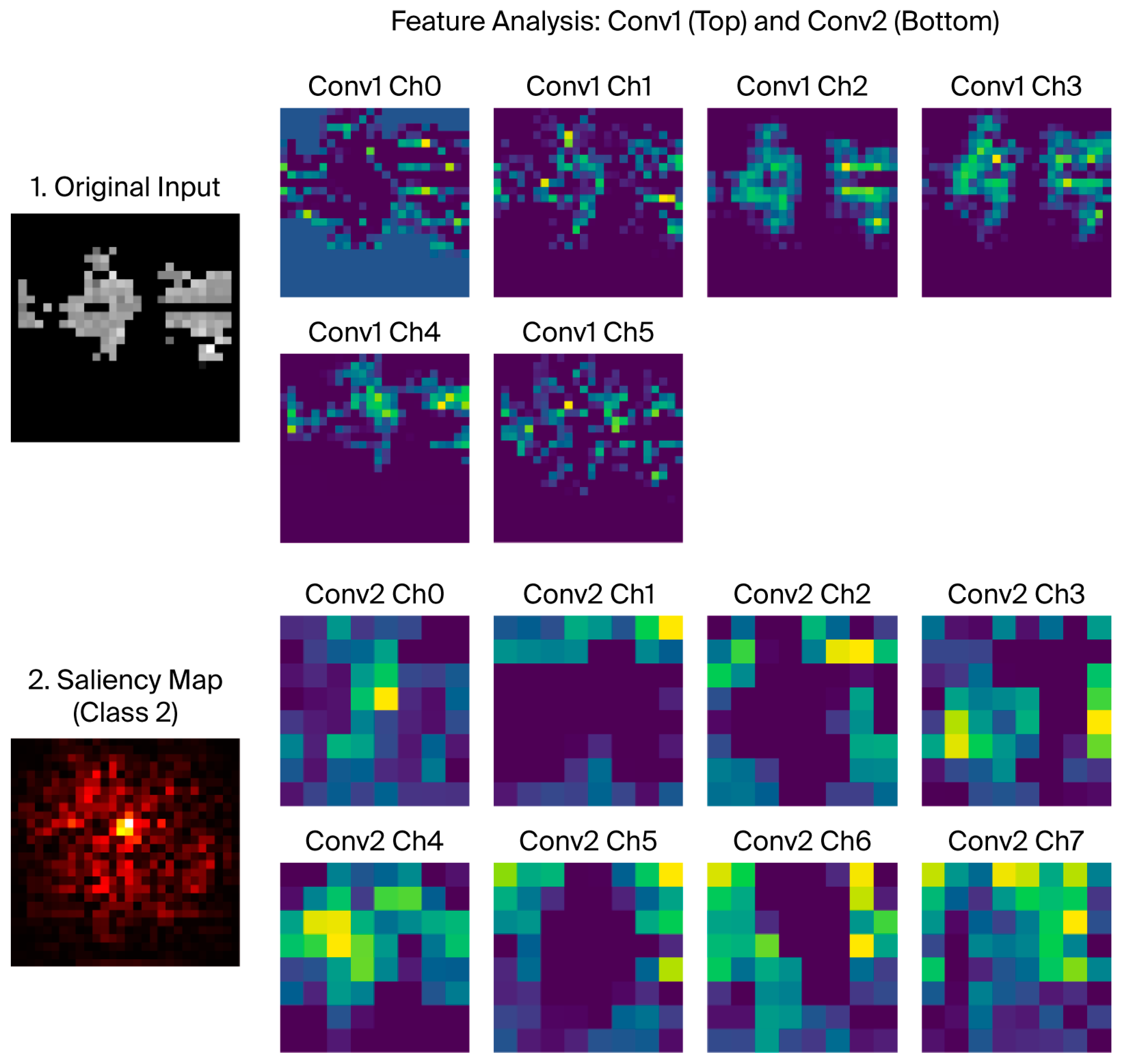
Table 5 lists the number of parameters and weights required for the different networks. ResNet-18 had the largest number of parameters and weights, although ShuffleNetV2 and MobileNetV2 reduced the number of parameters or weights by a factor of ten. However, the network from Ref. [13] is more lightweight than ShuffleNetV2 and MobileNetV2, and the confusion matrix in Table 6 shows that it also had the fewest misclassifications. Therefore, the network architecture proposed in this study, which combines Lanczos with the neural network from [13], is acceptable. Figure 8, Figure 9, Figure 10 and Figure 11 shows the saliency maps and feature maps for the different neural networks, providing a visual representation. The neural network architecture proposed in this study, as clearly shown in Figure 9, Figure 10 and Figure 11, has clearer saliency maps and feature maps than the other networks.

3.4. System Applicability and Overfitting Experimental Analysis

Based on the original dataset, three different types of noise (Additive Gaussian Noise, Uniform Noise, and Speech Noise), a 10-degree left–right rotation, and a ±5% signal shift were added, resulting in a total of seven different interference conditions. During training, each sample was randomly selected using one of these interference conditions to verify the robustness of the proposed model and to assess the risk of overfitting. Table 7 shows, similar to the confusion matrix in Table 2, that the method used in this study can still maintain nearly the same results under the different training and testing conditions with seven different types of interference. Therefore, it can be inferred that the model has stable performance under different interference conditions and that there is no risk of overfitting.

4. Conclusions

This paper proposes an integrated high-performance interpolation algorithm and a lightweight convolutional neural network for discharge detection. Considering data licensing factors, this study used publicly available generator discharge signal datasets. Although the sources differ from those of discharge signals generated by oil-impregnated paper bushings, the signal distribution is similar, allowing for a fair analysis and providing a reference for evaluating discharge signals generated by oil-impregnated paper bushings or other discharge devices. This network can be trained and applied to small sample datasets to identify partial discharge patterns in oil-impregnated paper bushings. It avoids overfitting caused by excessive extraction of training set features and achieves high scores in performance metrics such as accuracy and recall. More importantly, this network has a simple structure, few parameters, and low computational cost. Since training data for partial discharges in oil-impregnated paper bushings is difficult to obtain, this study used publicly available datasets to simulate approximate signals. The results can provide a reference for researchers with available data. Comparisons with several commonly used lightweight networks were performed, and the confusion matrix confirmed that this study’s proposed network achieved the best results. Compared to interpolation algorithms used in previous studies, it effectively improved the accuracy from 97% to 99%. This network was also successfully ported to embedded systems and, using validation data as input, was used to approximate the operating state of oil-impregnated paper bushings for online diagnostics, thereby enabling early warning of insulation defects and ensuring the safety of transmission lines.

Funding

This work was supported by the National Science and Technology Council (NSTC) in Taiwan under grant number 114-2222-E-130-002-.

Data Availability Statement

The original contributions presented in this study are included in the article. Further inquiries can be directed to the corresponding author.

Conflicts of Interest

The author declares no conflicts of interest.

References

  1. Chan, J.C.; Ma, H.; Saha, T.K.; Ekanayake, C. Stochastic noise removal on partial discharge measurement for transformer insulation diagnosis. In Proceedings of the 2014 IEEE PES General Meeting|Conference & Exposition, National Harbor, MD, USA, 27–31 July 2014; pp. 1–5. [Google Scholar] [CrossRef]
  2. Gulski, E. Digital analysis of partial discharges. IEEE Trans. Dielectr. Electr. Insul. 1995, 2, 822–837. [Google Scholar] [CrossRef]
  3. Feng, D.; Ke, C.; Wu, K. Simulation of Oil-Paper Sleeve Condition Assessment Based on Frequency Domain Dielectric Spectrum Analysis. Transfomer 2015, 52, 52–54. [Google Scholar] [CrossRef]
  4. Qin, X.; Qian, Y.; Xu, Y.; Sheng, G.; Jiang, X. Application of Feature Extraction Method Based on 2D-LPEWT in Cable Partial Discharge Analysis. Trans. China Electrotech. Soc. 2019, 34, 170–178. [Google Scholar] [CrossRef]
  5. Li, C.; Peng, X.; Ling, P.; Liu, T.; Zhou, J.; Zhang, Y. Phase resolved partial discharge patterns of typical defects from generator stators with different size of samples. In Proceedings of the 2024 IEEE International Conference on High Voltage Engineering and Applications (ICHVE), Berlin, Germany, 18–22 August 2024; pp. 1–4. [Google Scholar] [CrossRef]
  6. Zhu, Y.; Jia, Y.; Wang, L.; Li, L.; Zheng, Y.Y. Feature Extraction and Classification on Partial Discharge Signals of Power Transformers Based on Improved Variational Mode Decomposition and Hilbert Transform. Trans. China Electrotech. Soc. 2017, 32, 221–235. [Google Scholar] [CrossRef]
  7. Zhu, Y.; Yu, Y.; Chen, X.; Sheng, G.; Jiang, X. Pattern Recognition of Partial Discharges in DC XLPE Cables Based on Convolutional Neural Network. Trans. China Electrotech. Soc. 2020, 35, 659–668. [Google Scholar] [CrossRef]
  8. Song, H.; Dai, J.; Zhang, W.; Bi, K.; Sheng, G.; Jiang, X. Partial discharge pattern recognition based on deep convolutional networks under complex data sources. High Volt. Eng. 2018, 44, 3625–3633. [Google Scholar] [CrossRef]
  9. Li, Z.; Wang, J.; Zhou, X.; Huang, S.; Yan, R.; Xia, Z. Influence of chamber structure on arc quenching in multigap system. High Volt. Appar. 2020, 5, 313–318. [Google Scholar] [CrossRef]
  10. Wen, L.; Li, X.; Gao, L.; Zhang, Y. A New Convolutional Neural Network-Based Data-Driven Fault Diagnosis Method. IEEE Trans. Ind. Electron. 2018, 65, 5990–5998. [Google Scholar] [CrossRef]
  11. Liu, Y.; Pei, S.; Fu, W.; Zhang, K.; Ji, X.; Yin, Z. The discrimination method as applied to a deteriorated porcelain insulator used in transmission lines on the basis of a convolution neural network. IEEE Trans. Dielectr. Electr. Insul. 2017, 24, 3559–3566. [Google Scholar] [CrossRef]
  12. Jiang, J.; Bie, Y.; Li, J.; Yang, X.; Ma, G.; Lu, Y.; Zhang, C. Fault diagnosis of the bushing infrared images based on mask R-CNN and improved PCNN joint algorithm. High Volt. 2020, 6, 116–124. [Google Scholar] [CrossRef]
  13. Liu, Y.; Hu, M.; Dai, Q.; Le, H.; Liu, Y. Online recognition method of partial discharge pattern for transformer bushings based on small sample ultra-micro-CNN network. AIP Adv. 2021, 11, 045221. [Google Scholar] [CrossRef]
  14. Getreuer, P. Linear Methods for Image Interpolation. Image Process. Line 2011, 1, 238–259. [Google Scholar] [CrossRef]
  15. Henao, J.D.Z.; Tamayo, H.A.T.; Segura, J.A.J.; Diaz, H.; Paz, A. Images of Resolved Phase Patterns of Partial Discharges in Electric Generators. Mendeley Data. Version 8. 2023. Available online: https://data.mendeley.com/datasets/xz4xhrc4yr/8 (accessed on 16 February 2026).
  16. AMD Zynq™ Evaluation Kit. Available online: https://xilinx-wiki.atlassian.net/wiki/spaces/A/pages/189530183/Zynq-7000 (accessed on 16 February 2026).
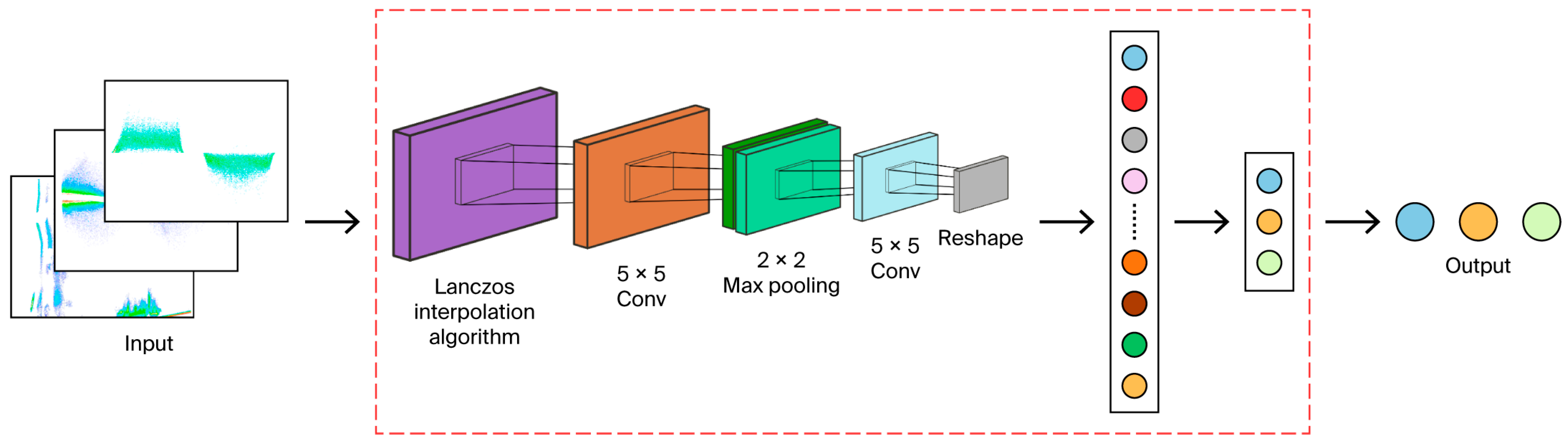
Figure 1. The diagram illustrates the lightweight CNN architecture proposed in this study.
Electronics 15 01584 g001
Figure 2. PRPD spectrum characteristics of different defect types: (a) PRPD type 1, (b) PRPD type 2.
Electronics 15 01584 g002
Figure 3. PRPD spectrum characteristics of corona defect types at different resolutions: (a) 570 × 440, (b) 28 × 28. The obtained pulse patterns are represented in RGB color, which aids in assessing the repeatability of pulses across their distribution.
Electronics 15 01584 g003
Figure 4. PRPD spectrum characteristics of internal defect types at different resolutions: (a) 570 × 440, (b) 28 × 28. The obtained pulse patterns are represented in RGB color, which aids in assessing the repeatability of pulses across their distribution.
Electronics 15 01584 g004
Figure 5. PRPD spectrum characteristics of surface defect types at different resolutions: (a) 570 × 440, (b) 28 × 28. The obtained pulse patterns are represented in RGB color, which aids in assessing the repeatability of pulses across their distribution.
Electronics 15 01584 g005
Figure 6. The output partial discharge signal was set to the signal mode measured by the sensor. (a) Original database. (b) 570 × 440 resolution converted to 1 × (570 × 440) output points.
Electronics 15 01584 g006
Figure 7. Partial discharge signal output by Zynq 7000 series embedded system. Verification results are displayed on oscilloscope.
Electronics 15 01584 g007
Figure 8. ShuffleNetV2 saliency maps and feature maps for different channels and network layers. It tells us the degree to which each pixel in the image affects the image’s classification score.
Electronics 15 01584 g008
Figure 9. MobileNetV2 saliency maps and feature maps for different channels and network layers. It tells us the degree to which each pixel in the image affects the image’s classification score.
Electronics 15 01584 g009
Figure 10. ResNet-18 saliency maps and feature maps for different channels and network layers. It tells us the degree to which each pixel in the image affects the image’s classification score.
Electronics 15 01584 g010
Figure 11. Proposed method’s saliency maps and feature maps for different channels and network layers. It tells us the degree to which each pixel in the image affects the image’s classification score.
Electronics 15 01584 g011
Table 1. Training, validation, and testing data allocation for different PD types.
PRPD TypeTraining Set
(70%)
Validation Set
(15%)
Testing Set
(15%)
Total
Corona4319293616
Internal4269291609
Surface4429595632
Table 2. Performance metrics for different types of partial discharge and different types of interpolation methods combined with neural networks [13].
PRPD TypePrecision (%)Recall (%)F1 Score (%)
Input 28 × 28 via Nearest Neighbor down sampling
Corona100.0100.0100.0
Internal98.995.697.2
Surface95.998.997.4
Input 28 × 28 via Bilinear down sampling
Corona98.9100.099.5
Internal100.097.898.9
Surface99.0100.099.5
Input 28 × 28 via Bicubic down sampling
Corona98.9100.099.5
Internal98.997.898.3
Surface98.998.998.9
Input 28 × 28 via B-Spline down sampling
Corona100.0100.0100.0
Internal98.995.697.2
Surface95.998.997.4
Input 28 × 28 via Lanczos down sampling (proposed method)
Corona100.0100.0100.0
Internal97.8100.098.9
Surface100.097.998.9
Table 3. Confusion matrix of different types of interpolation methods combined with neural networks [13].
PRPD TypeCoronaInternalSurface
Input 28 × 28 via Nearest Neighbor down sampling
Corona9300
Internal0871
Surface0494
Input 28 × 28 via Bilinear down sampling
Corona9310
Internal0890
Surface0195
Input 28 × 28 via Bicubic down sampling
Corona9310
Internal0891
Surface0194
Input 28 × 28 via B-Spline down sampling
Corona9300
Internal0871
Surface0494
Input 28 × 28 via Lanczos down sampling (proposed method)
Corona9300
Internal0912
Surface0093
Table 4. Comparison of computation time for different interpolation methods and neural network combinations.
InterpolationCNN
ShuffleNetV2MobileNetV2ResNet-18[13]
42 ms39 ms531 ms34 ms
Nearest43.7440.29532.4135.73
Bilinear46.7144.29536.3239.28
Bicubic50.4447.95539.9043.01
Lanczos57.0354.55547.6549.67
Table 5. Comparison of neural network parameters and weights of different interpolation methods and neural network combinations.
InterpolationCNN
ShuffleNetV2MobileNetV2ResNet-18[13]
Neural network parameter counts1,256,2472,227,13911,171,77928,883
Weight size4.96 MB8.73 MB42.6 MB117 KB
Table 6. Confusion matrix for different types of partial discharge.
PRPD TypeCoronaInternalSurface
ShuffleNetV2
Corona741613
Internal106021
Surface91561
MobileNetV2
Corona773617
Internal123716
Surface41862
ResNet-18
Corona9300
Internal0861
Surface0594
[13]
Corona9300
Internal0871
Surface0494
Table 7. Performance metrics for different types of partial discharges and different types of interpolation methods combined with neural networks (with training and testing with various types of noise interference).
PRPD TypeCoronaInternalSurface
Input 570 × 440
Corona51703
Internal39724193
Surface1884564
Input 28 × 28 via Nearest Neighbor down sampling
Corona52214
Internal49715200
Surface17312556
Input 28 × 28 via Bicubic down sampling
Corona534010
Internal74716153
Surface13612597
Input 28 × 28 via B-Spline down sampling
Corona54301
Internal26714192
Surface17514567
Input 28 × 28 via Lanczos down sampling (proposed method)
Corona560022
Internal64720120
Surface1208618
Disclaimer/Publisher’s Note: The statements, opinions and data contained in all publications are solely those of the individual author(s) and contributor(s) and not of MDPI and/or the editor(s). MDPI and/or the editor(s) disclaim responsibility for any injury to people or property resulting from any ideas, methods, instructions or products referred to in the content.