Ensemble Graph Neural Networks for Probabilistic Sea Surface Temperature Forecasting via Input Perturbations

Abstract

Accurate regional ocean forecasting requires models that are both computationally efficient and capable of representing predictive uncertainty. This work investigates ensemble learning strategies for sea surface temperature (SST) forecasting using Graph Neural Networks (GNNs), with a focus on how input perturbation design affects forecast skill and uncertainty representation. We adapt a GNN architecture to the Canary Islands region in the North Atlantic and implement a homogeneous ensemble approach inspired by bagging, where diversity is introduced during inference by perturbing initial ocean states rather than retraining multiple models. Several noise-based ensemble generation strategies are evaluated, including Gaussian noise, Perlin noise, and fractal Perlin noise, with systematic variation of noise intensity and spatial structure. Ensemble forecasts are assessed over a 15-day horizon using deterministic metrics (RMSE and bias) and probabilistic metrics, including the Continuous Ranked Probability Score (CRPS) and the Spread–skill ratio. The results show that, while deterministic skill remains comparable to the single-model forecast, the type and structure of input perturbations influence uncertainty representation, particularly at longer lead times. Ensembles generated with spatially coherent perturbations, such as low-resolution Perlin noise, achieve improved calibration and lower CRPS compared to purely random Gaussian perturbations. These findings highlight the role of noise structure and scale in ensemble GNN design, indicating that specifically structured input perturbations can improve ensemble diversity and calibration without additional training cost. These results provide a methodological contribution toward the study of ensemble-based GNN approaches for regional ocean forecasting.

1. Introduction

The increasing relevance of the blue economy [1], the accelerating impacts of climate change, and the objectives defined within the Sustainable Development Goals have intensified the demand for accurate and timely ocean forecasting systems [2]. Reliable predictions of oceanographic variables, such as sea surface temperature (SST), are essential for maritime operations, ecosystem monitoring, fisheries management, and climate-related decision-making. Traditionally, these forecasts have relied on numerical ocean models that explicitly solve the physical equations governing ocean dynamics. While physically grounded and robust, such models are computationally expensive and often restricted to large operational centers, limiting their accessibility and adaptability to regional and high-resolution applications [3].

Recent advances in machine learning (ML) have introduced an alternative paradigm for geophysical prediction, enabling data-driven models to learn complex spatiotemporal relationships directly from observations and reanalysis products [4]. Leveraging modern hardware accelerators, ML-based models offer orders-of-magnitude faster inference compared to numerical solvers, making them particularly attractive for operational and near-real-time forecasting. Although many state-of-the-art ML climate models operate at global scales, recent work has demonstrated their growing potential for regional applications, where higher spatial resolution is required to capture localized ocean processes such as coastal upwelling and mesoscale variability.

Within this context, Graph Neural Networks (GNNs) have emerged as a powerful framework for modeling geophysical systems defined over irregular spatial domains [5]. By representing spatial locations as nodes and their physical relationships as edges, GNNs naturally handle complex geometries such as coastlines and bathymetry, which are difficult to model using regular grids. Architectures such as GraphCast [6] and its regional adaptations [7] have demonstrated that GNNs can achieve competitive or superior performance to traditional numerical models in medium-range forecasting while maintaining high computational efficiency. Recent works [8,9] extend this approach to regional ocean prediction through a hierarchical encoder–processor–decoder GNN tailored to oceanographic data.

Despite these advances, a major limitation of most deep learning-based forecasting systems is their deterministic nature, which hampers their ability to represent forecast uncertainty—an essential component for operational oceanography and climate services [10]. Ensemble forecasting [11] is the standard approach for uncertainty quantification in numerical weather and ocean prediction, typically achieved through perturbed initial conditions or stochastic parameterizations. Recently, ensemble methodologies have also been adopted in machine learning-based forecasting systems, including AIFS ENS [12], GenCast [13], NeuralGCM [14], and Pangu-Weather [15], demonstrating that ML ensembles can provide calibrated probabilistic forecasts at a fraction of the computational cost of traditional ensemble systems.

Ensemble learning relies fundamentally on diversity among its members: individual forecasts must differ sufficiently so that their errors are weakly correlated, allowing aggregation to improve robustness and reliability [16,17]. In the context of deep learning, diversity can be introduced through heterogeneous architectures, multiple independently trained models, or perturbations applied to inputs, parameters, or latent representations. However, training multiple high-capacity models is often computationally prohibitive, particularly for regional GNNs operating on high-resolution meshes.

This work explores a computationally efficient ensemble strategy for regional ocean forecasting using GNNs, implemented through input perturbation during inference rather than repeated training. Building on SeaCast [8], we adapt the model to the Canary Islands region in the North Atlantic, and investigate how different noise-based perturbation strategies affect ensemble performance. Specifically, we compare Gaussian noise and spatially structured perturbations based on Perlin and fractal Perlin noise, systematically analyzing the influence of noise intensity and spatial resolution.

The ensemble forecasts are evaluated using both deterministic metrics (RMSE and bias) and probabilistic metrics from WeatherBench [18], including the Continuous Ranked Probability Score (CRPS) and the spread–skill ratio. These metrics allow us to assess not only forecast accuracy but also ensemble calibration and uncertainty representation across multiple lead times. By focusing on inference-time perturbations and ensemble design choices, this study aims to clarify how uncertainty can be effectively represented in GNN-based regional ocean forecasts through lightweight ensemble construction.

In contrast to recent generative or multi-model ensemble approaches, this work focuses on lightweight ensemble construction aimed at reducing computational overhead in high-resolution GNN-based forecasting systems. Rather than retraining multiple networks or introducing stochasticity during training, we investigate how structured perturbations of the initial ocean state at inference time can induce forecast diversity while relying on a single trained model. This design enables ensemble generation from a single model and serves as a proof-of-concept for obtaining probabilistic information without the need for multiple independently trained models.

The main contributions of this work are threefold: First, we present an efficient ensemble framework for regional SST forecasting based on inference-time input perturbations applied to a hierarchical GNN; second, we provide a systematic comparison of unstructured (Gaussian) versus spatially coherent (Perlin and fractal Perlin) noise, showing that the latter is associated with more stable uncertainty estimates at longer lead times; third, we offer empirical guidance on noise scale and structure for ensemble GNN design in regional ocean applications.

The remainder of the paper is organized as follows: Section 2 reviews related work on ML-based geophysical forecasting and ensemble methods; Section 3 describes the dataset, GNN architecture, and ensemble generation strategies; Section 4 outlines the experimental setup and evaluation metrics; Section 5 presents the results; and Section 6 discuss the implications of our findings and conclude with directions for future research.

2. Related Work

Ensemble forecasting is central to uncertainty quantification in numerical weather prediction (NWP), where diversity is typically introduced through perturbed initial conditions and stochastic parameterizations. As ML models increasingly complement or replace traditional solvers in atmospheric and ocean forecasting, ensemble methodologies have been adapted to neural architectures [19] to provide probabilistic predictions. Recent work in ML-based geophysical forecasting can be organized into four principal ensemble paradigms: (i) independently trained multi-model ensembles, (ii) generative probabilistic models, (iii) hybrid physics–ML systems with stochastic components, and (iv) inference-time perturbation ensembles.

Operational AI systems such as AIFS ENS [12] follow the classical ensemble paradigm by training or fine-tuning multiple model instances. Diversity arises from independent optimization trajectories, initialization differences, or data subsampling, consistent with ensemble theory [16,20,21]. This strategy benefits from strong variance reduction and often yields well-calibrated forecasts. However, it requires substantial computational resources, limiting scalability for regional, high-resolution domains where training multiple large neural models is prohibitive.

A second paradigm is represented by diffusion-based systems such as GenCast [13]. These models learn the conditional distribution of future states and directly generate multiple coherent forecast trajectories. By optimizing distributional objectives, they achieve competitive CRPS performance relative to operational ensemble systems. Nevertheless, generative approaches [22,23,24] introduce considerable training complexity, high computational costs, and reduced interpretability, as uncertainty is encoded implicitly in latent representations rather than explicitly through physically motivated perturbations.

NeuralGCM [14] exemplifies a hybrid strategy in which neural components are embedded within a physically inspired dynamical core. Stochastic perturbations are applied to learned tendencies, and probabilistic losses such as CRPS guide training. This approach enhances physical consistency and uncertainty representation but increases architectural complexity and coupling between model components, complicating adaptation to irregular regional meshes and ocean-specific geometries.

Recent work highlights the importance of spatially coherent perturbations. Pangu-Weather [15] demonstrated that structured Perlin noise [25] applied to initial states can generate meaningful ensemble diversity while preserving spatial smoothness. Compared to spatially independent Gaussian perturbations, structured noise better respects geophysical correlation scales, reducing artificial high-frequency artifacts. However, prior studies have primarily focused on global atmospheric forecasting and have not systematically examined how perturbation resolution and scale influence probabilistic skill, particularly in regional ocean contexts.

In parallel, GNNs [26,27] have emerged as powerful tools for geophysical prediction [5,28] on irregular domains [29,30]. Systems such as GraphCast [6] demonstrate that encoder–processor–decoder GNN architectures achieve state-of-the-art medium-range forecasting skill with high computational efficiency. Yet these models are predominantly deterministic, and ensemble strategies for GNN-based geophysical forecasting remain underexplored. Broader GNN ensemble approaches introduce diversity via architectural variation or subgraph sampling [31,32], but these strategies typically require retraining and are not tailored to probabilistic forecasting metrics.

Existing ensemble paradigms reveal a trade-off: generative and multi-model systems offer strong probabilistic calibration but incur high computational cost, while simple perturbation schemes are inexpensive but may lack physical realism. This work explores homogeneous ensembles for hierarchical GNNs [7,33] in regional sea surface temperature forecasting [8,9,34], introducing diversity exclusively at inference time through controlled perturbations of the initial ocean state. We provide a systematic comparison between unstructured Gaussian noise and spatially coherent Perlin-based perturbations, explicitly analyzing the impact of noise structure and resolution on CRPS and spread–skill ratio [18,35,36]. Our results suggest that spatial coherence plays a key role in achieving well-calibrated medium-range forecasts, while the effect of perturbation complexity appears to be secondary under the evaluated configurations.

By focusing on structured inference-time perturbations within a regional GNN framework, this study proposes a lightweight approach to probabilistic ocean forecasting, exploring the trade-off between deterministic neural models and more resource-intensive generative ensemble systems in a computationally efficient setting.

3. Methods and Data

3.1. Dataset

This study relies on three primary data types: oceanographic, atmospheric forcing, and bathymetry. Oceanographic data were obtained from the Copernicus Marine Service (CMEMS), specifically the European North-West Shelf/Iberia–Biscay–Irish Seas High-Resolution L4 Sea Surface Temperature Reprocessed product. This Level 4 reanalysis merges satellite observations with quality control and gap-filling, providing consistent daily SST data from 1 January 1982 to 31 December 2023, at 0.05° × 0.05° resolution over the North Atlantic, Bay of Biscay, Irish Sea, and part of the western Mediterranean. The spatial domain is bounded by the coordinates listed in

Table 1. Coordinates delimiting the area of study.

Parameter	Value
Maximum latitude	34.525°
Minimum latitude	19.55°
Maximum longitude	−5.975°
Minimum longitude	−20.97°

. SST is measured at 20 cm depth, with an accompanying error field (not used for model training, as this study focuses on evaluating ensemble uncertainty generated through perturbations rather than propagating observational uncertainty). Data were processed into daily matrices. Figure 1 shows the SST for 1 January 2018, in our domain.

Atmospheric forcing data were obtained from the Copernicus Climate Data Store (C3S) ERA5 hourly data on single levels (1940–present). Two variables were selected: the east–west ($u10$) and north–south ($v10$) components of 10 m wind speed. Data were aggregated to daily means and interpolated to the CMEMS SST grid using bilinear interpolation, without the application of additional smoothing or filtering. The resulting fields were stored as daily arrays of ocean points. Figure 2 shows u and v winds for 1 January 2018.

Bathymetry data were obtained from NOAA’s ETOPO Global Relief Model 2022, providing ocean depth and land elevation at 0.0083° resolution. Depths were extracted for the study area, resampled to the SST grid, and land values were set to zero. Figure 3 shows the processed bathymetry.

3.2. Graph Neural Network: Adapting to the North-Atlantic Subregion

SeaCast is a GNN designed for high-resolution, medium-term ocean predictions. The model leverages the complex geometry of the oceans through an autoregressive approach that combines historical oceanographic states, external forcings, and static information to predict future states. Originally developed for the Mediterranean Sea, it has been adapted in this study to the North Atlantic region.

It formalizes the prediction problem using temporal windows. Let the historical states of the oceanographic variables be denoted as

$$X^{-h:0}=(X^{-h},\dots ,X^0),$$

where $X^{-h}$ represents the state h days in the past and $X^0$ the current state. The future prediction window is

$$X^{1:T}=(X^1,\dots ,X^T),$$

where T denotes the prediction horizon in days. Forcing factors are defined analogously as

$$F^{1:T}=(F^1,\dots ,F^T).$$

The prediction relies on four components: initial and target states, forcings, and static data. The initial states consist of the previous day and the current value, while the target states correspond to the oceanographic variables over the T forecasted days. In this study, we set $T=1$ for training and validation, and $T=15$ for testing. During training, the model only requires one day of forcing information, as it is trained to predict one time step ahead. Thanks to its autoregressive design, predictions can be extended to any length T by sequentially generating states ${\widehat{X}}^{1:T}$, starting from $X^0$. Figure 4 illustrates the autoregressive process.

The forecasting model used in this work was intentionally selected without autoregressive steps, as preliminary experiments showed only minor performance differences compared to a model trained with four autoregressive steps, while exhibiting substantially lower computational cost. A comparison between single-step and four-step autoregressive configurations is provided in Appendix A, confirming the small performance gap between both approaches.

The purpose of this work is not to optimize the forecasting model itself, but to analyze the effects of ensemble perturbation strategies on a fixed baseline. Using a single-step trained model allows us to isolate and study the impact of different noise configurations on prediction diversity without introducing additional variability from model retraining. However, this choice implies that the model is not specifically optimized for long autoregressive horizons, and therefore, results at longer lead times should be interpreted with caution.

While this may accumulate errors in autoregressive prediction, as observed in medium-range weather forecasting systems such as Pangu-Weather [15], all compared ensemble configurations are evaluated under the same rollout procedure. Therefore, any bias induced by long-horizon propagation affects all methods equally, preserving the validity of relative comparisons between ensemble strategies.

In this work, SeaCast is used as a fixed baseline model, and no modifications are introduced to its core architecture. The changes applied are limited to domain adaptation to the North Atlantic region and adjustments required by computational constraints. Therefore, the focus of this study is placed on the analysis of ensemble perturbation strategies applied to a fixed forecasting backbone, rather than on model design.

SeaCast employs an encoder–processor–decoder architecture on a hierarchical mesh graph [7], where each stage uses an independent interaction network [37] to capture relationships between nodes and external influences. Inputs from the latitude–longitude grid are first projected onto the hierarchical mesh by the encoder, processed through sequential updates of latent representations in the processor, and finally mapped back to the grid by the decoder. The model predicts residual changes at each grid cell as:

$${\widehat{X}}_r^t=X_r^{t-1}+{\mathrm{MLP}}^{\mathrm{pred}}\left(v_r^G\right),$$

(1)

where $v_r^G$ is the latent graph representation of cell r obtained from the mesh-to-grid connections. This residual formulation improves training stability and prediction accuracy while preserving the core GNN architecture.

To adapt the model to the North Atlantic, we made the following changes:

• Input constants were modified to accommodate new data sources, grid dimensions, and the number of oceanographic and atmospheric variables.
• The hierarchical mesh was adapted to the north-west African coast, including the Canary Islands.
• The mesh consists of three resolution levels (81, 27, 9 nodes per side), with the finest level including 81 × 81 nodes.
• Nodes and edges crossing land were removed, resulting in a total of 38,714 nodes and 49,061 grid-to-mesh connections.
• The number of neighbors per node in the hierarchy was reduced from 16 to 1 to improve computational efficiency.
• The processor includes four GNN layers, and hidden vector representations in the GNNs and MLPs have a dimension of 128.
• Training was performed on a single GPU with 32 GB RAM, requiring sequential processing of daily data and limiting batch size to one.
• Autoregressive steps were initially increased from one to four, but later reduced to one in the final training to reduce computational cost.
• A noise module was introduced to generate diverse ensemble predictions.
• Evaluation tools from WeatherBench were modified to handle the custom data format.
• The final model included ∼5.6 million trainable parameters.

These modifications allow efficient operation in the North Atlantic while maintaining the core GNN architecture and autoregressive prediction capabilities. The model was trained to minimize the Mean Squared Error (MSE), considering the sequence of states generated by autoregressive steps, also known as rollout. The loss function is given by:

$$L={\displaystyle \frac{1}{T_{\mathrm{rollout}}}}\sum _{t=1}^{T_{\mathrm{rollout}}}\sum _{i=1}^C\sum _{l=1}^{L_i}{\displaystyle \frac{1}{\left|G_l\right|}}\sum _{v\in G_{l\left(i\right)}}{a}_v{\lambda }_i{\left({\widehat{X}}_{v,i}^t-X_{v,i}^t\right)}^2,$$

(2)

where $T_{\mathrm{rollout}}$ is the number of autoregressive steps, C is the total number of variables, $L_i$ is the number of depth levels of feature i, and $G_l$ represents the number of grid points in the ocean at level l. The term $a_v$ represents the weighting according to cell size, calculated as the cosine of latitude for each cell v and depth level l. Finally, ${\lambda }_i$ is the inverse of the variance of the estimates for variable i [8].

3.3. Ensemble Method

Our ensemble learning strategy combines multiple models to generate a prediction during inference. This approach, inspired by the wisdom of the crowd, relies on the expectation that individual model errors will partially cancel out, yielding more accurate predictions than a single model. The outputs are combined using an aggregation function [20].

For an ensemble to outperform an individual model, base models must be better than random, and their errors should be as independent as possible [16]. Diversity among models is crucial: heterogeneous ensembles use different architectures (e.g., Stacking), while homogeneous ensembles use identical architectures with variations in inputs or parameters.

In this study, we adopted a bagging-inspired homogeneous ensemble strategy. Instead of retraining multiple models on bootstrapped datasets, a single GNN model is employed, and diversity is introduced at inference time by perturbing the oceanographic input data with noise. Predictions generated from perturbed initial states are aggregated through their mean to produce the final forecast. The types of noise and their characteristics are described in the following subsections.

It is important to note that this ensemble strategy primarily captures initial-condition uncertainty. All ensemble members share the same model parameters; therefore, model uncertainty associated with parameter estimation is not represented. The focus of this study is to evaluate how different types and configurations of input noise affect prediction diversity, rather than to construct a full ensemble covering all sources of uncertainty.

3.3.1. Gaussian

The simplest approach to introducing variability into the data is by adding random perturbations drawn from a normal distribution. Gaussian noise is widely used due to its prevalence in natural processes and favorable statistical properties. The distribution is given by

$$p\left(x\right)={\displaystyle \frac{1}{\sqrt{2\pi {\sigma }^2}}}{e}^{-\frac{{(x-\mu )}^2}{2{\sigma }^2}},$$

(3)

where $\mu$ denotes the mean and ${\sigma }^2$ the variance. Gaussian noise has been employed in several state-of-the-art climate modeling frameworks included in performance benchmarks [36], such as ArchesWeatherGen [22], NeuralGCM [14], FuXi [38], and FourCastNet [39].

Figure 5 illustrates the effect of varying the standard deviation of the sampling distribution on noise intensity, assuming zero mean in all cases. A standard deviation of 1 yields perturbations that can reach values close to 4 in the distribution tails, whereas a standard deviation of 0.5 produces noticeably lower-amplitude noise due to reduced dispersion. When the standard deviation is set to 0.1, the perturbations become barely perceptible at the shared visualization scale. Despite these differences in magnitude, all realizations exhibit a spatially uncorrelated structure, resulting in uniformly scattered patterns across the domain.

3.3.2. Perlin Noise

In the context of ensemble construction, Perlin noise [25] offers a structured approach to promoting diversity while preserving spatial correlations. In contrast to Gaussian noise, which introduces spatially independent perturbations, Perlin noise generates smooth variations with controllable correlation lengths determined by the selected spatial resolution. This property enables the creation of ensemble members that differ in a physically consistent manner, maintaining large-scale coherence while introducing localized variability. Consequently, this type of noise facilitates diversification without injecting spurious high-frequency artifacts, making it particularly suitable for perturbing geophysical variables characterized by strong spatial dependencies. Perlin noise has been notably applied in Pangu-Weather [15] to generate random perturbations.

To generate the noise, a three-dimensional grid is first considered, whose points have integer coordinates. These points, which act as the vertices of the grid cubes, are assigned pseudo-random values and gradient vectors through a hash function H, which produces four mutually independent real values. For a point with coordinates $(x,y,z)$, this assignment is represented by the following equation:

$$[a,b,c,d]=H(x,y,z),$$

(4)

where a, b and c represent the gradient and d the value of the function at the point $(x,y,z)$.

If the evaluated point $(x,y,z)$ coincides with a grid point, then the noise value equals d. Otherwise, if the point lies within the volume bounded by the vertices of a cube, the noise is computed through smooth interpolation (e.g., a cubic polynomial) using the values and gradients of the surrounding vertices. This interpolation is performed first along the x-axis (between edges), then along the y-axis (across cube faces), and finally along the z-axis (between planes). This procedure allows the generation of noise with a spatial component.

Figure 6 shows two different Perlin noise configurations that differ in the spatial resolution applied. In the case of higher spatial resolution on the latitude and longitude axes (2, 12, 12), a greater number of noise patterns can be observed, while in the low-resolution configuration (2, 3, 3), the patterns are larger and it is clearer to see how the interpolation smooths the transitions within each cell. Another important feature is that the higher resolution noise has a slightly higher intensity.

3.3.3. Fractal Perlin Noise

Another alternative for generating noise is the fractal Perlin noise. This function is distinguished by the use of three additional parameters. The first is octaves, which represent the number of iterations of the noise. Then there is persistence, which acts as the scaling factor for the noise amplitude between consecutive octaves. Finally, lacunarity is the factor of increase in frequency between two octaves. Its equation is given as:

$$F(x,y,z)=\alpha ·\sum _{i=0}^{O-1}{a}_i·H(x,y,z;f_i),$$

(5)

where $\alpha$ represents the noise scale, O represents the number of octaves, $a_i$ is the noise amplitude, and $f_i$ is the frequency that modifies the resolution. The lacunarity, persistence, and resolution evolve as follows:

$${\mathrm{resolution}}_i=f_i·{\mathrm{resolution}}_0;f_i=\mathrm{lacunarity}·f_{i-1};a_i=\mathrm{persistence}·a_{i-1}.$$

(6)

The noise resolution applied in each octave must always be an exact divisor of the dimensions of the desired noise shape.

Figure 7 shows two different configurations of fractal Perlin noise that differ only in the spatial resolution applied. Three octaves are used in the noise iteration, with a persistence of 0.5, which means that the intensity decreases progressively with each iteration. The lacunarity is two, which means that as the octaves progress, smaller and smaller patterns are used, resulting in more detailed and complex noise. In addition, a noise scalability coefficient ($\alpha =0.2$) is applied to the noise resulting after the last octave.

4. Experimental Setup

4.1. Evaluation Metrics

Two sets of metrics are used in this study: probabilistic metrics to evaluate the ensemble predictions generated from noisy inputs, and classical deterministic metrics, such as RMSE or Bias, to compare predictions against a single model without noise. This section focuses on the probabilistic metrics.

Table 2. Notation used in the metrics [36].

Symbol	Rank	Description
f	-	Prediction
o	-	Observation
t	$1,\dots ,T$	Verification time
l	$1,\dots ,L$	Prediction horizon
i	$1,\dots ,I$	Latitude index
j	$1,\dots ,J$	Longitude index
m	$1,\dots ,M$	Set member index

summarizes the notation used throughout the metric definitions.

The CRPS evaluates the accuracy of ensemble predictions, balancing the error against the internal dispersion of the set. For individual members X and observation Y, the CRPS is given by

$${\mathrm{CRPS}}_{\mathrm{skill}}=\mathbb{E}|X-Y|,$$

(7)

$${\mathrm{CRPS}}_{\mathrm{spread}}=\mathbb{E}[X-X^{\prime }],$$

(8)

$$\mathrm{CRPS}={\mathrm{CRPS}}_{\mathrm{skill}}-{\displaystyle \frac{1}{2}}{\mathrm{CRPS}}_{\mathrm{spread}}=\mathbb{E}|X-Y|-{\displaystyle \frac{1}{2}}\mathbb{E}|X-X^{\prime }|.$$

(9)

The CRPS used in this study accounts for all set members and verification times [35] and is calculated as

$${\mathrm{CRPS}}_l:={\displaystyle \frac{1}{T}}\sum _t^T\left({\displaystyle \frac{1}{M}}\sum _{m=1}^M{∥f^{\left(m\right)}-o∥}_{t,l}-{\displaystyle \frac{1}{2M(M-1)}}\sum _{m=1}^M\sum _{\begin{array}{c}n=1\\ n\ne m\end{array}}^M{∥f^{\left(m\right)}-f^{\left(n\right)}∥}_{t,l}\right).$$

(10)

The first term of the metric measures the average error of ensemble members relative to observations, and the second term provides an unbiased estimate of internal dispersion to correct for finite ensemble size.

The Spread–Skill Ratio evaluates ensemble calibration by comparing the ensemble dispersion to the RMSE of the ensemble mean. The spread is defined as

$${\mathrm{Spread}}_l=\sqrt{{\displaystyle \frac{1}{TIJ}}\sum _t^T\sum _i^I\sum _j^J{\mathrm{var}}_m\left(f_{t,l,i,j,m}\right)},$$

(11)

with the variance of ensemble members given by

$${\mathrm{var}}_m\left(f_{t,l,i,j,m}\right)={\displaystyle \frac{1}{M-1}}\sum _{m=1}^M{\left(f_{t,l,i,j,m}-{\overline{f}}_{t,l,i,j}\right)}^2.$$

(12)

The spread–skill ratio is calculated as follows:

$$R_l={\displaystyle \frac{{\mathrm{Spread}}_l}{{\mathrm{RMSE}}_l\left(\overline{f}\right)}}.$$

(13)

A value of $R_l\approx 1$ indicates good calibration, where ensemble dispersion reflects the actual prediction error. Values greater than one indicate overestimated uncertainty, while values below one indicate insufficient ensemble variability. Unlike CRPS, which balances error and dispersion, the spread–skill ratio directly measures the calibration of the ensemble [40,41].

In this work, a bias-corrected RMSE is used to reduce systematic errors when calculating the spread–skill ratio, providing a more reliable estimate of ensemble calibration.

4.2. Implementation

The preprocessing pipeline consists of organizing the raw atmospheric, oceanographic, and static data into structured samples based on predefined date ranges for training, validation, and testing. Each sample includes two initial ocean states and the corresponding forcing variables. Before training, all input variables are normalized using precomputed mean and standard deviation values derived from the training set. Static features such as bathymetry and spatial coordinates are also incorporated as additional inputs.

Noise is introduced during the data loading stage by adding perturbations to the initial ocean states only, while forcing variables remain unchanged. Each ensemble member corresponds to a different random realization of the noise, ensuring variability in the predictions.

The code used in this study is publicly available at: https://github.com/Alejeglez/ensemble-gnn-sst, accessed on 5 April 2026.

The Python (version 3.10.16) implementation adds Gaussian noise to each grid point using numpy.random.normal() (NumPy version 1.26.4), with configurable mean and standard deviation. Perlin noise is generated using the Python library perlin-numpy available at: https://github.com/pvigier/perlin-numpy, accessed on 5 April 2026.

4.3. Training Procedure

We employed a training period spanning 21 years of data with the dataset divided as follows: training data from 2003 to 2019 (17 years), validation data from 2020 to 2021 (2 years), and test data from 2022 to 2023 (2 years). This corresponds to approximately 81% of the data for training and 9.5% for validation and testing.

The model was trained using the AdamW optimizer with parameters ${\beta }_1=0.9$, ${\beta }_2=0.95$, and weight decay $\lambda =0.1$. The initial learning rate was set to $1\times {10}^{-5}$, with five warm-up epochs and a cosine decay schedule to progressively adjust the learning rate.

Network hyperparameters were selected as follows: hidden layers of 128 neurons, resulting in 128-dimensional vector representations within the GNNs and associated MLPs; four processing layers in the model processor; and a hierarchical mesh with three uniform levels at resolutions of 81, 27, and 9, respectively. Training was conducted for 150 epochs without autoregressive steps due to computational constraints.

The training environment consisted of a desktop workstation with an Intel Core i9-9900K processor (3.60 GHz, 8 cores, 16 threads), 32 GB of RAM, and an NVIDIA GeForce RTX 3060 GPU with 12 GB of VRAM, which enabled efficient handling of large datasets and accelerated computation.

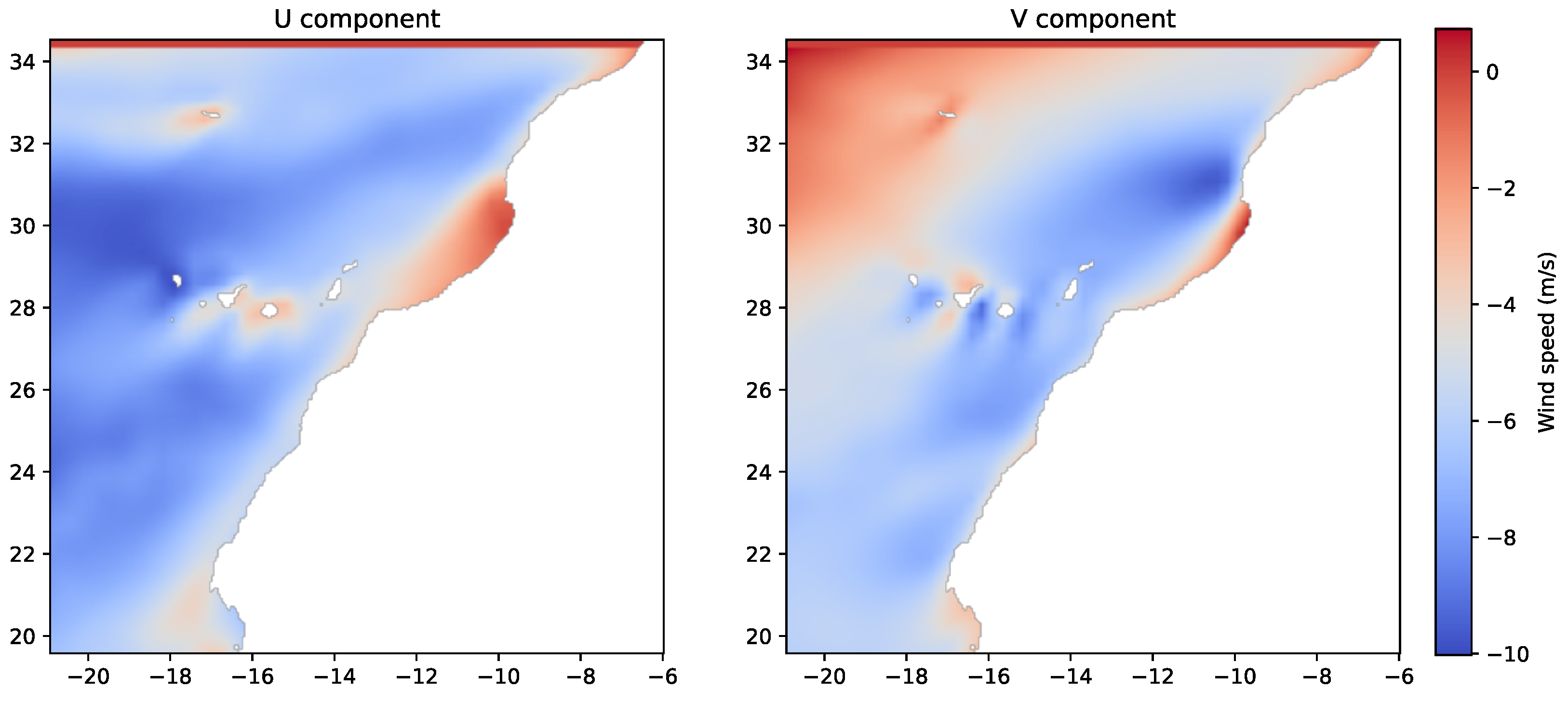
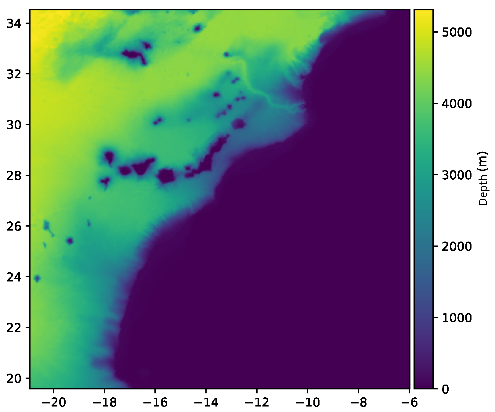
Before training, static features, such as bathymetry, coordinates, and normalization statistics, were computed, and differences between consecutive states were normalized to facilitate residual learning. The structure of the hierarchical mesh and bipartite connections were generated and stored for efficient access.

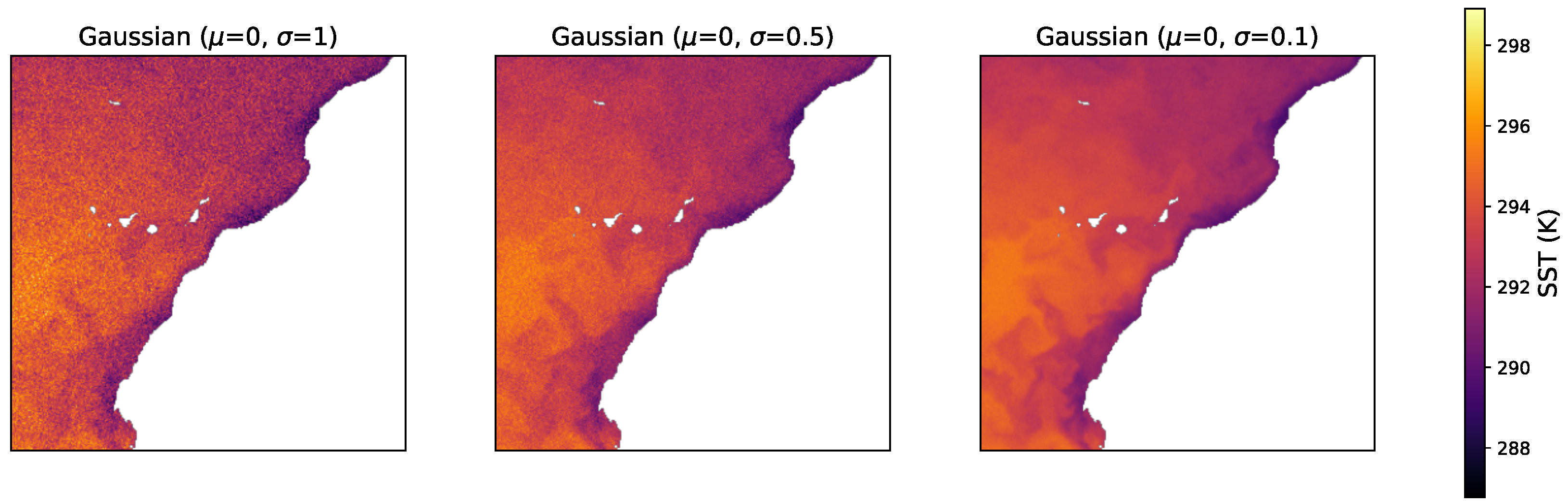
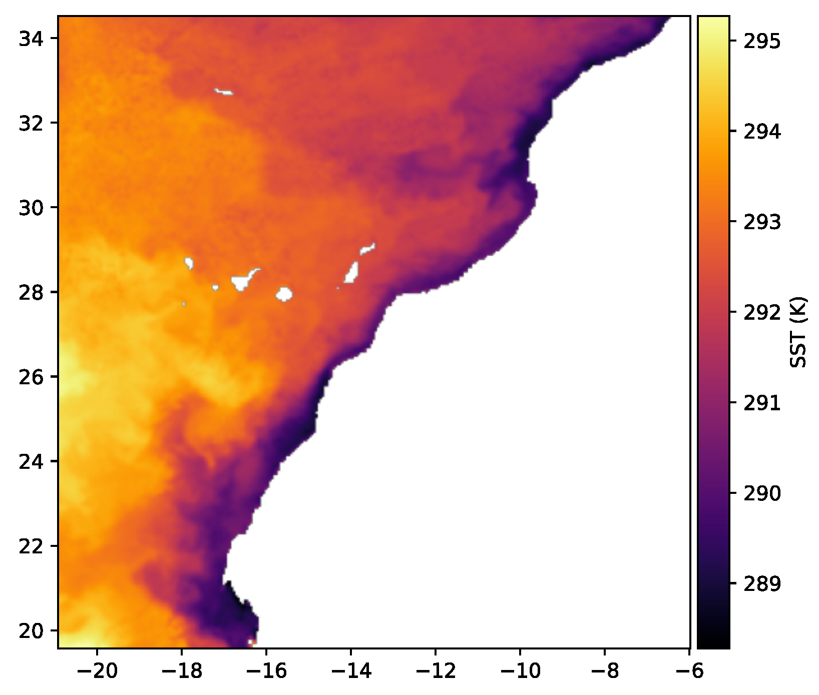
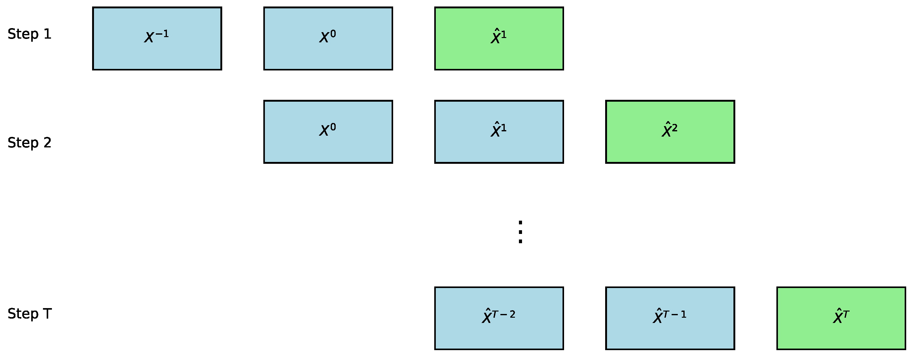
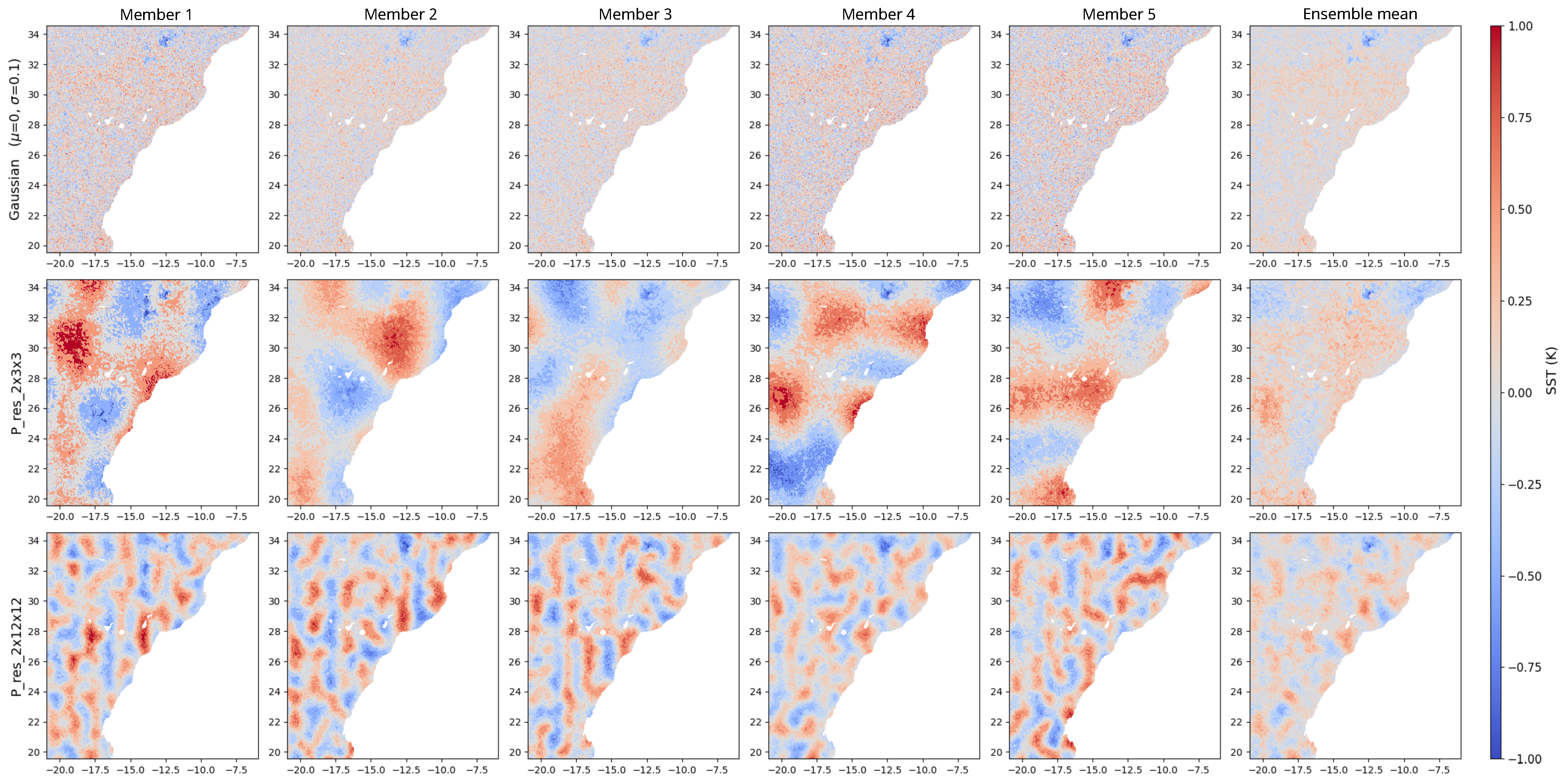
During training, the model learns to predict one-step-ahead oceanographic states. For evaluation, ensemble predictions are generated by introducing diversity in the initial states through noise perturbations (Gaussian, Perlin, and Perlin fractal). The ensemble predictions are then aggregated via daily averages, enabling both probabilistic and deterministic assessment of model performance.

4.4. Test Configurations

A preliminary parameter calibration phase was conducted before the ensemble experiments to define suitable noise configurations and to ensure a structured and reproducible exploration of the parameter space. Rather than performing a dense grid search, we adopt a controlled sensitivity analysis strategy aimed at sampling representative regions of each noise family.

In this phase, candidate parameter values for each noise type were evaluated based on their impact on forecast accuracy. Specifically, a one-factor-at-a-time approach was employed, in which each parameter was varied while the remaining ones were kept fixed, allowing us to isolate its individual effect. Each configuration was evaluated by computing the RMSE at each forecast lead time for 29 randomly selected initialization dates, drawn using a fixed random seed to ensure reproducibility, and then averaging across initialization dates to obtain a representative RMSE curve as a function of lead time.

This procedure defines a parameter screening stage, in which an initial set of candidate values is explored and a reduced number of representative configurations is selected for the subsequent ensemble experiments. The selection is guided by RMSE performance and aims to retain configurations that capture distinct behavioral regimes while avoiding redundancy.

The goal of this study was not to perform an exhaustive exploration of the full parameter space, but to compare qualitatively different types of perturbations under practical computational constraints. Therefore, the selected configurations should be understood as representative cases designed to illustrate differences in noise structure and behavior.

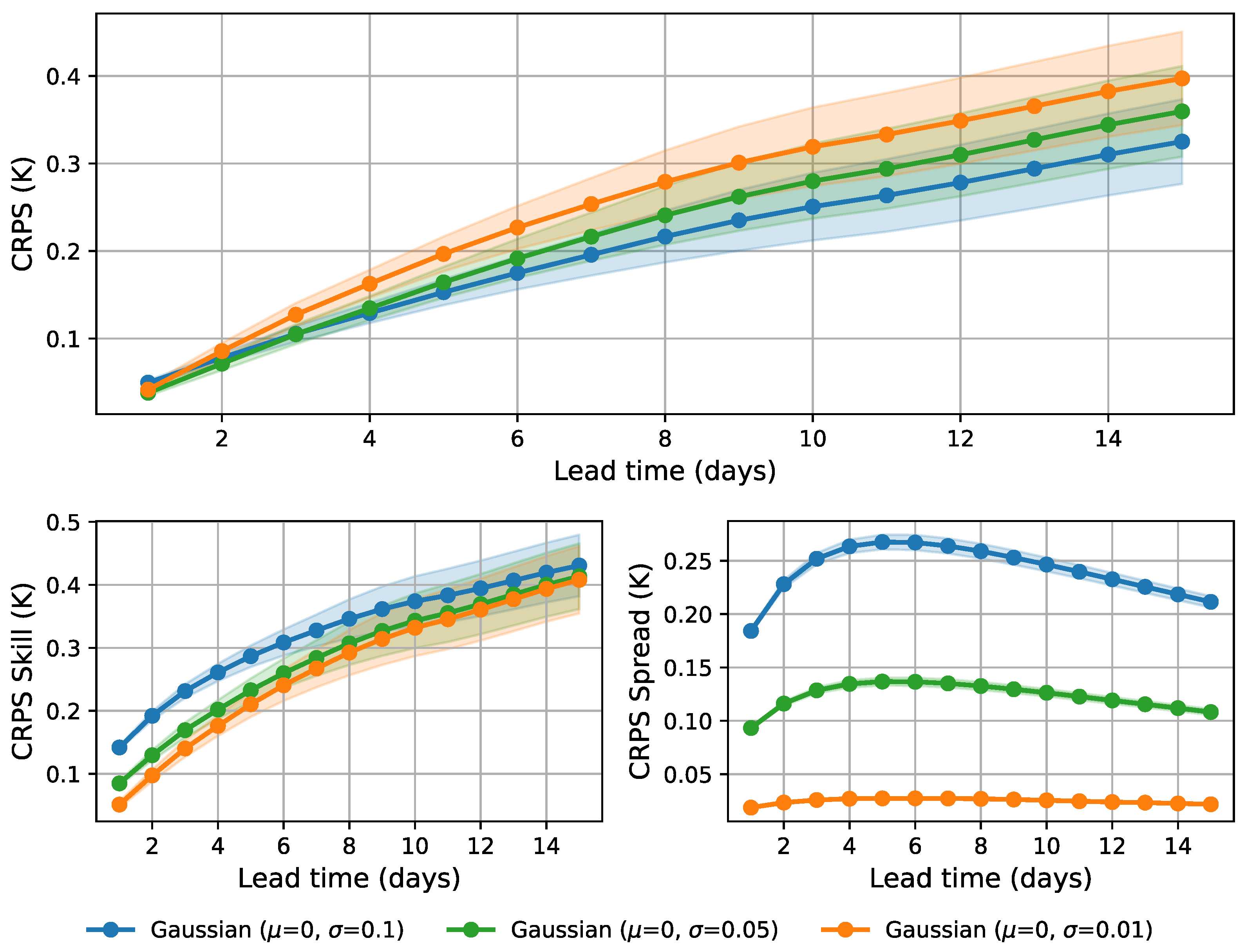
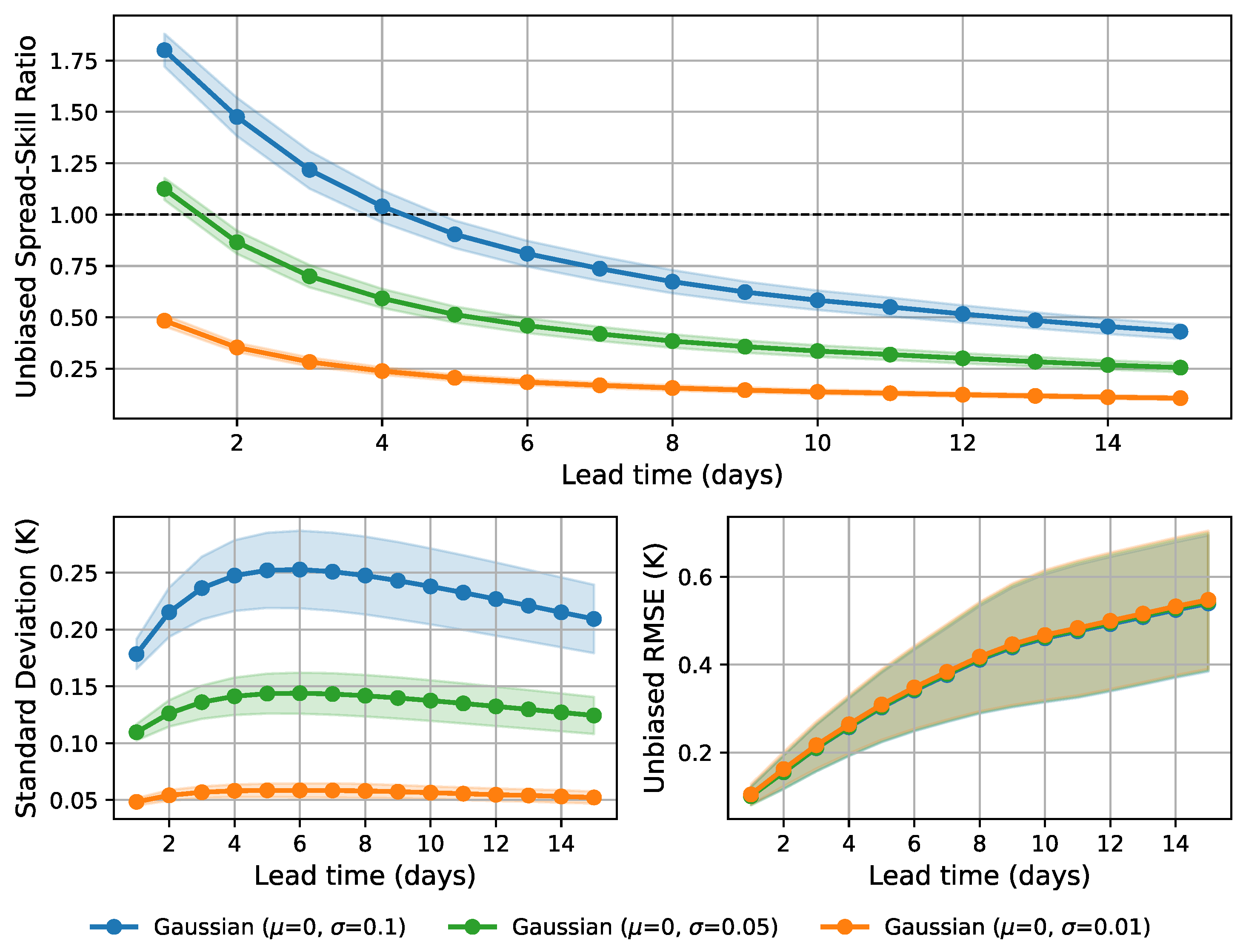
In addition, the parameter values were chosen such that the overall noise intensity remained roughly comparable across Gaussian and Perlin-based perturbations. This allows the comparison to focus on structural differences rather than differences in magnitude. For the Gaussian noise model, the standard deviation of the noise distribution was the only parameter considered for exploration, as it directly controls the amplitude of the perturbations.

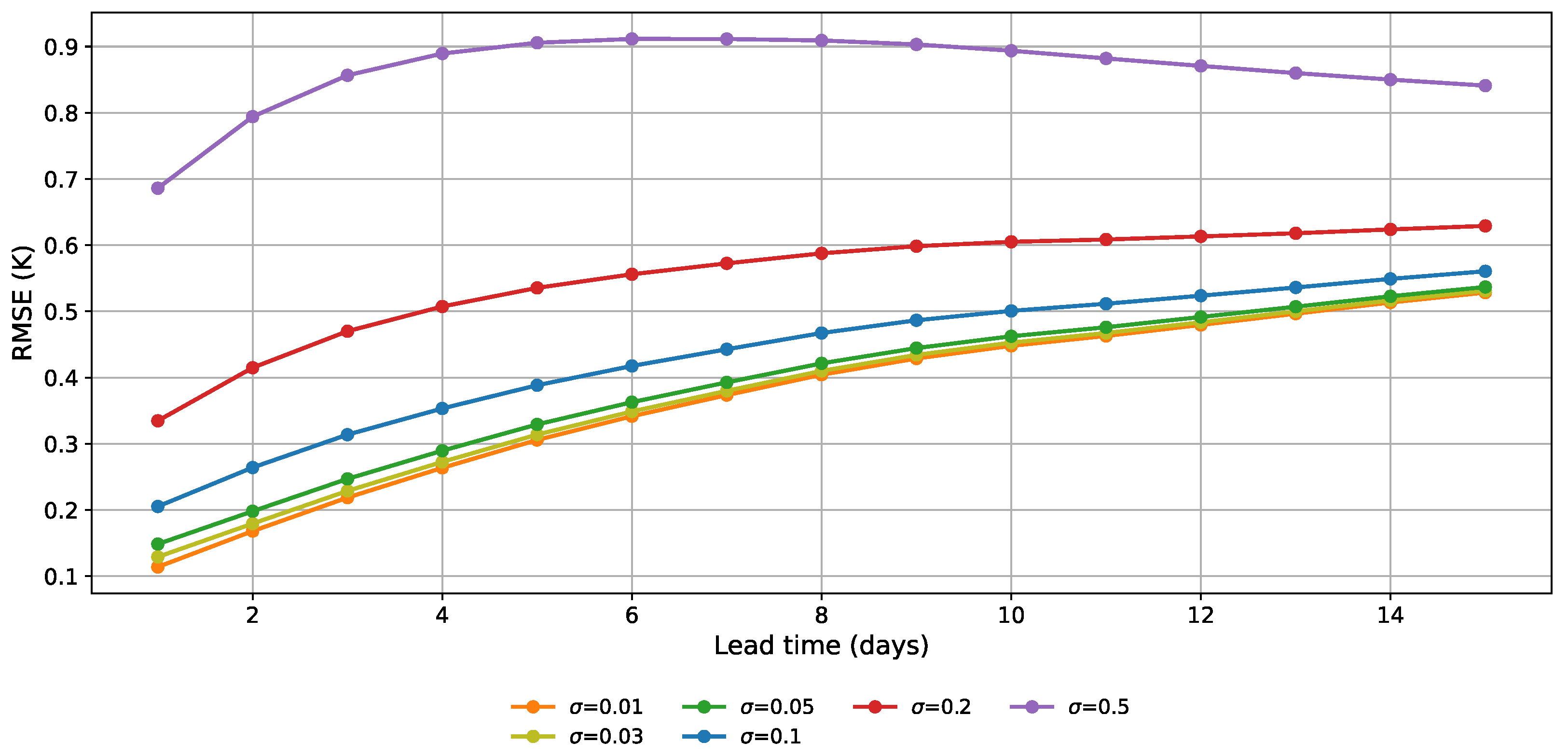
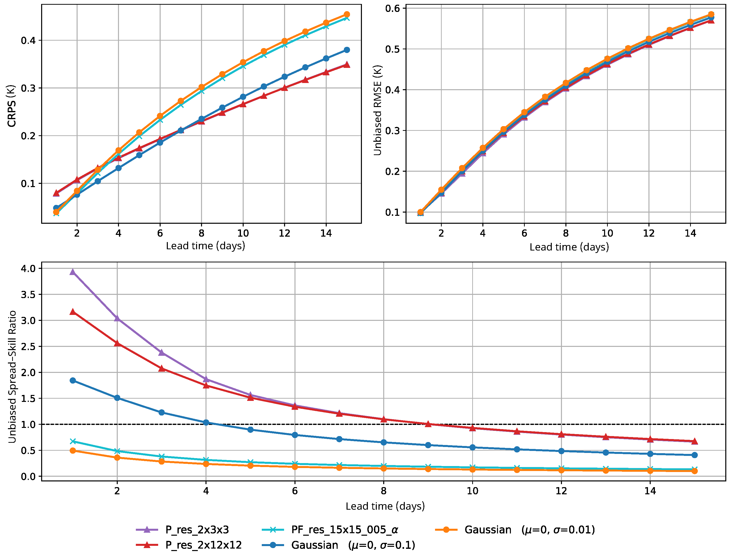
The standard deviations used ($\sigma$ = 0.01, 0.03, 0.05, 0.1, 0.2, 0.5) correspond to approximately 0.5%, 1.4%, 2.3%, 4.5%, 9.1%, and 22.7% of the observed SST variability in the study region (standard deviation ≈ 2.2 K). These values were selected as part of an initial systematic exploration of the Gaussian noise amplitude, spanning a wide range of perturbation regimes from weak to strongly forced conditions.

As shown in Figure 8, the best RMSE performance is consistently obtained for the lowest noise amplitudes. A gradual degradation of forecast skill is observed as the standard deviation increases, with a noticeable change in slope around $\sigma =0.1$, beyond which performance deteriorates more rapidly, and a stronger increase in error is observed for $\sigma \ge 0.2$.

Based on this behavior, the selected configurations ($\sigma$ = 0.01, 0.05, 0.1) are chosen to represent low to intermediate noise amplitudes within the explored range. In particular, $\sigma =0.01$ and $\sigma =0.05$ correspond to weak or near-deterministic perturbations, while $\sigma =0.1$ lies at the upper end of the low-noise regime. The selected Gaussian configurations are summarized in

Table 3. Gaussian noise configurations used during the tests.

Noise Type	Mean ($\mathit{\mu }$)	Standard Deviation ($\mathit{\sigma }$)
Gaussian ($\mu$ = 0, $\sigma$ = 0.1)	0.0	0.1
Gaussian ($\mu$ = 0, $\sigma$ = 0.05)	0.0	0.05
Gaussian ($\mu$ = 0, $\sigma$ = 0.01)	0.0	0.01

.

For the Perlin noise model, two parameters are considered: the spatial scale of the noise and the tileability constraint. The spatial scale is controlled by the number of grid subdivisions used to generate the noise field, which determines the size of the resulting spatial structures. The tileability parameter is set to enforce spatial continuity along the latitude dimension, ensuring coherent perturbations across domain boundaries. Spatial coherence is enforced by construction through the tileability constraint.

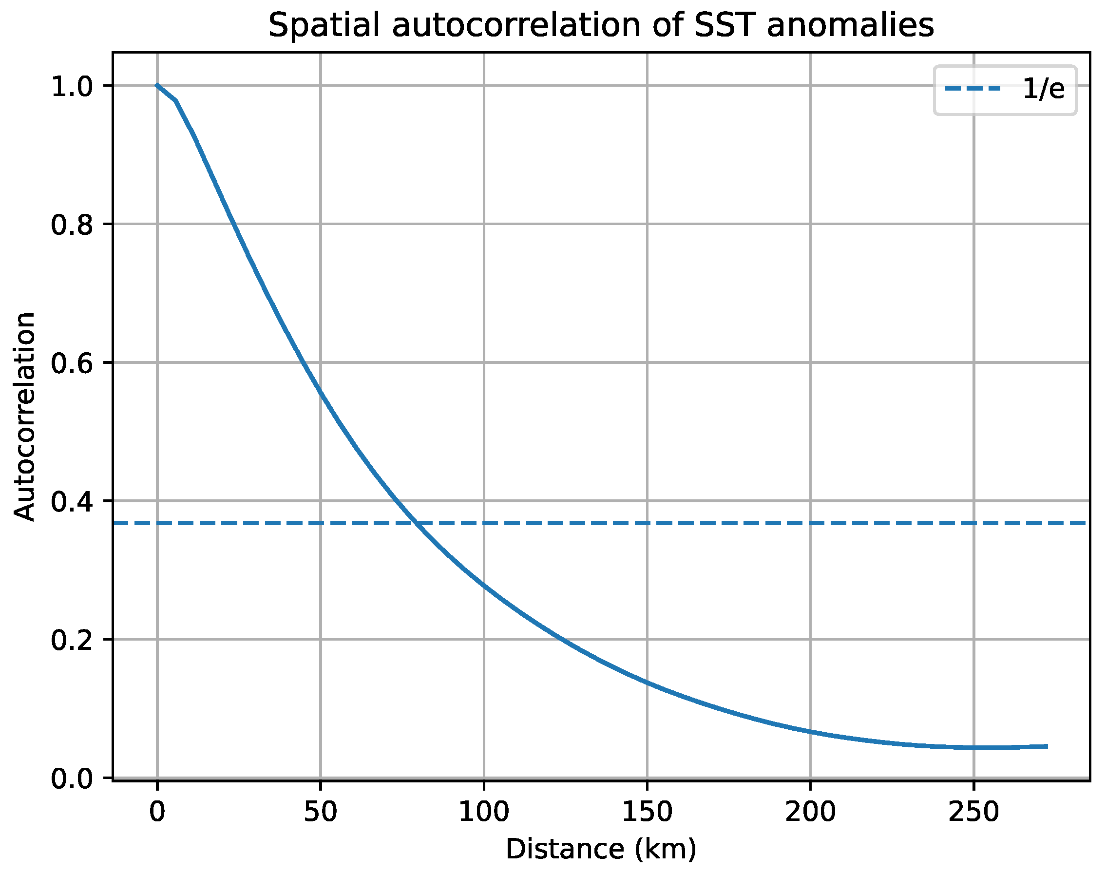
The resolutions of the Perlin noise were chosen based on the spatial autocorrelation structure and characteristic spatial scales of the SST field in the study region. Analysis of SST anomalies derived from the CMEMS product at 0.05° × 0.05° resolution indicates a dominant spatial scale of approximately 15 pixels (≈83 km), as shown in Figure 9.

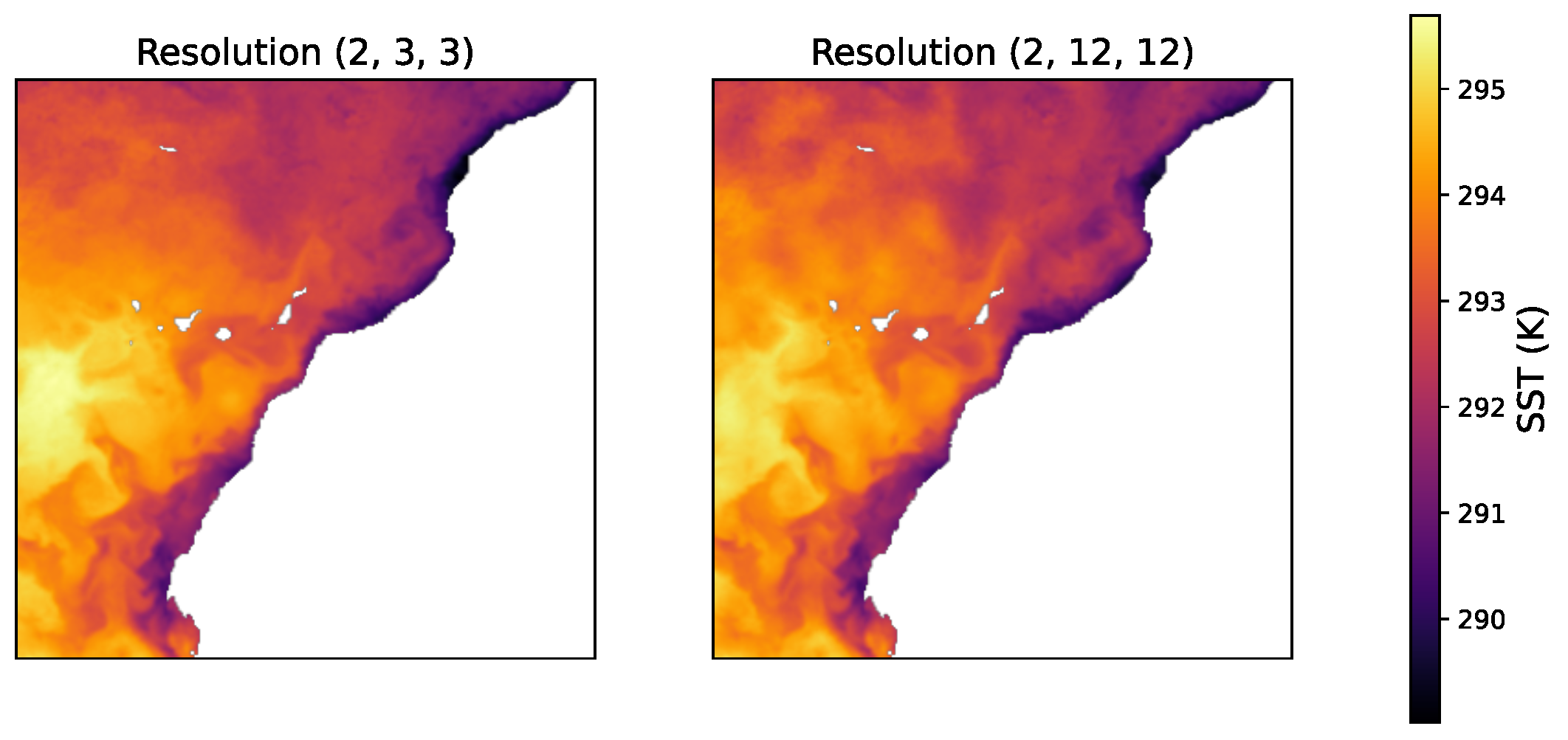
A configuration with 15×15 resolution on the 300 × 300 pixel domain generates perturbations of roughly 20 pixels (≈111 km), comparable in magnitude to the observed SST structures. This ensures that the noise captures physically meaningful spatial patterns. The classic Perlin noise configuration with 12 × 12 resolution produces slightly larger and coarser patterns, allowing evaluation of the effect of pattern size and density on forecast performance. A 3 × 3 base Perlin noise was also included to test very coarse, low-detail patterns.

Based on this physical constraint, the explored configurations are defined by varying the number of spatial subdivisions (3, 5, 6, 12, 15, and 25), which correspond to progressively finer spatial scales. This range spans scales both larger and smaller than the dominant SST variability (15 pixels), enabling a structured exploration of how the noise field interacts with physically relevant spatial scales.

The tileability parameter was also evaluated under a fixed-resolution setting (2 × 6 × 6) to assess its potential influence. However, no significant differences were observed in forecast performance between tileable and non-tileable configurations, suggesting a limited impact within the considered experimental setup. As a result, tileability is not further considered in the remainder of the study.

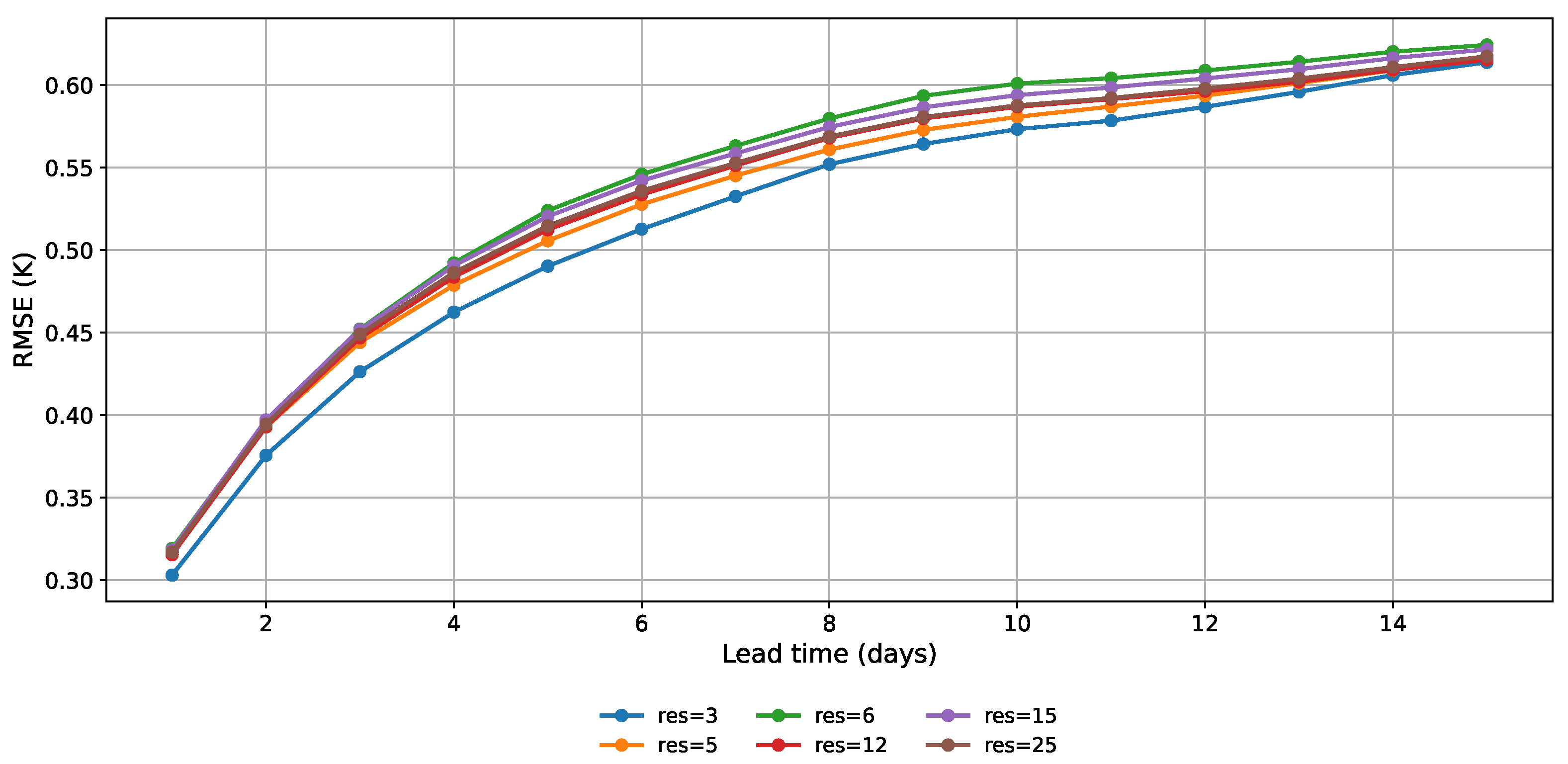
The RMSE analysis, as shown in Figure 10, indicates that the coarsest configuration (3 subdivisions) yields slightly better performance at early forecast lead times. However, no monotonic relationship is observed between spatial scale and forecast error. In particular, the finest-scale configuration does not consistently exhibit the worst performance, and intermediate and fine-scale configurations produce comparable RMSE values. As lead time increases, differences across configurations further diminish, indicating a weak sensitivity of forecast skill to the spatial scale of the perturbations.

Based on this behavior, two representative configurations (3 × 3 and 12 × 12 resolutions) are selected for the subsequent evaluation stage. These configurations are chosen to represent contrasting levels of spatial detail: a coarse-scale regime characterized by large spatial structures, and an intermediate-scale regime with finer variability. In addition, they differ from the resolution configurations selected for the fractal Perlin noise model, enabling a clearer comparison between noise types. The selected Perlin configurations are summarized in

Table 4. Classic Perlin noise configurations used during the tests.

Noise Type	Resolution	Repeatable
P_res_2x3x3	(2, 3, 3)	(T, F, F)
P_res_2x12x12	(2, 12, 12)	(T, F, F)

, where we use the following systematic naming scheme:

• Classic Perlin noise uses P_res_XxYxZ, where XxYxZ indicates the spatial resolution along each dimension.
• Fractal Perlin noise uses PF_res_XxY, where XxY indicates the 2D spatial resolution. Optional modifications are added as suffixes: ($\alpha$=value) indicates a modified scale factor applied to the noise.

For the fractal Perlin noise configurations, three parameters are explored: spatial resolution, tileability, and noise scale ($\alpha$). As in the previous configurations, the tileability constraint does not lead to noticeable differences in the spatial structure of the perturbations under the considered experimental setup and is therefore not further explored in detail.

The baseline configuration is derived from the setup proposed in Pangu-Weather [15], which uses a fractal Perlin noise with 15 × 15 spatial resolution, three octaves, persistence of 0.5, lacunarity of 2, and a noise scale of 0.2. In this study, octaves, persistence, and lacunarity are kept fixed to the recommended values from Pangu-Weather to preserve the multi-scale structure of the noise and isolate the effect of the selected control parameters.

Spatial resolutions are chosen to ensure compatibility with the iterative octave construction, where each successive octave modifies the effective spatial scale according to the lacunarity factor. Given the 300 × 300 domain, the studied configurations (5 × 5, 15 × 15 and 25 × 25) are designed to be compatible with the domain discretization and the previous spatial analysis, while providing a comparable setting to the base Perlin configurations.

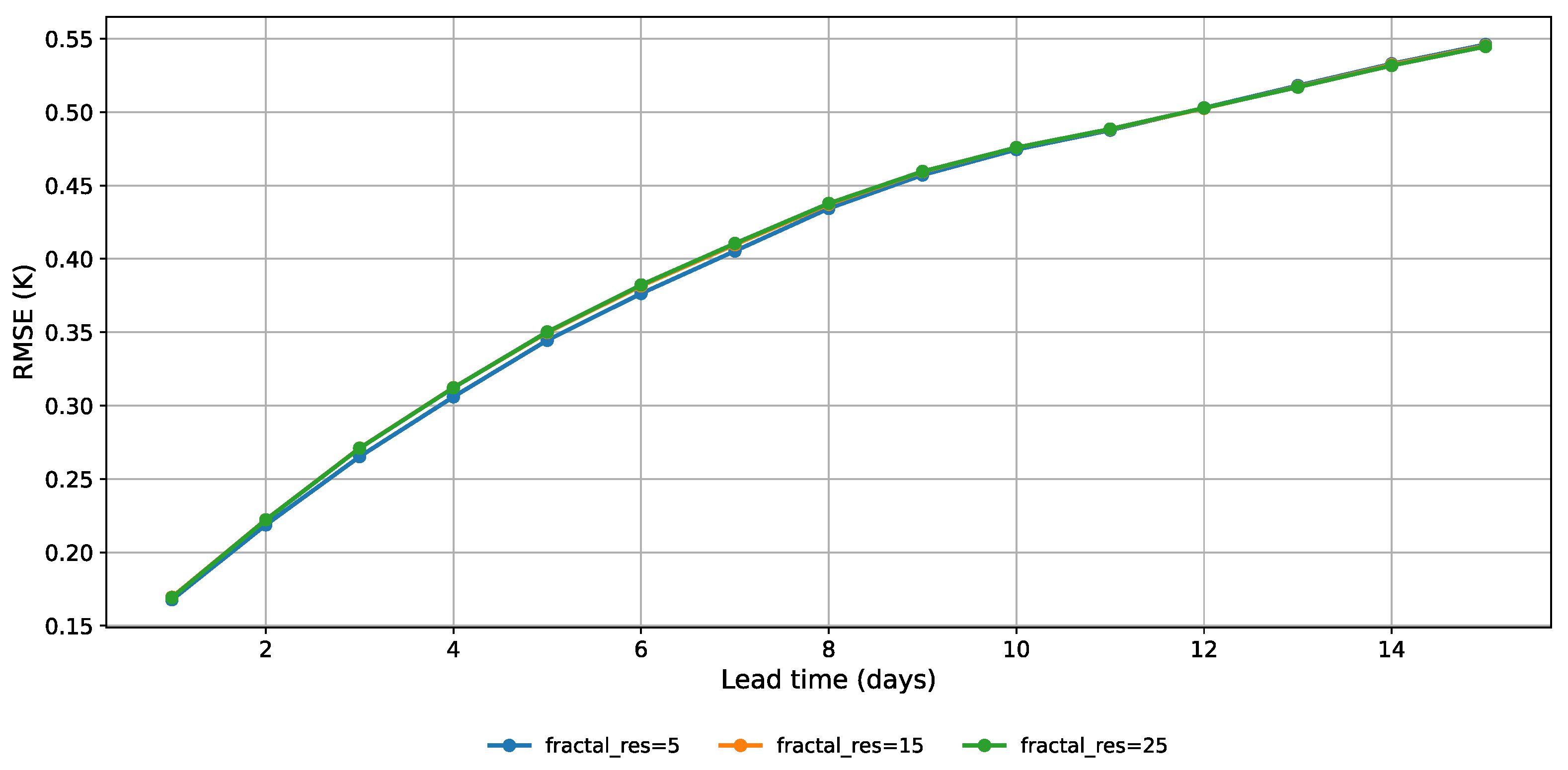
Unlike standard Perlin noise, which can be formulated in a fully spatio-temporal (3D) framework, the implementation used here is purely two-dimensional in space. Due to the octave-based construction, the noise field is generated independently for each temporal state, and therefore, no explicit coherence is enforced between noise realizations at consecutive time steps. However, as shown in Figure 11, the RMSE analysis does not reveal a consistent sensitivity to resolution within this range, indicating that performance differences are not strongly driven by spatial resolution, as was also observed for the base Perlin configuration. Accordingly, the final analysis focuses on two representative resolutions: 5 × 5 and 15 × 15, corresponding respectively to higher and lower levels of spatial subdivision within the tested range.

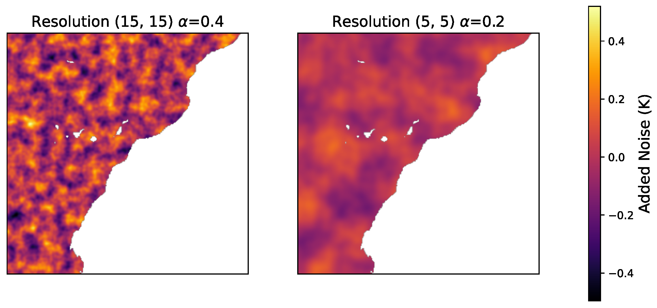
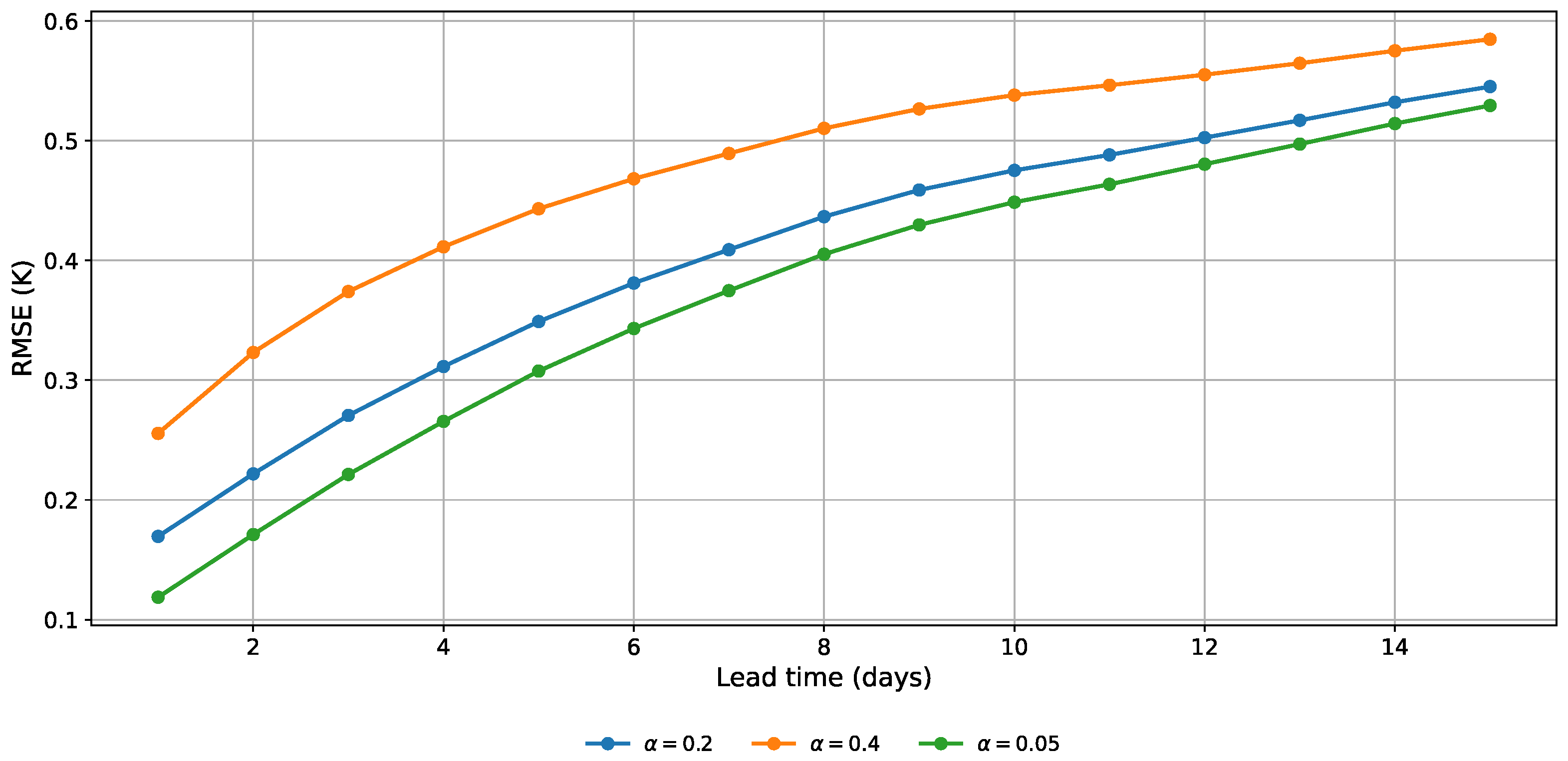
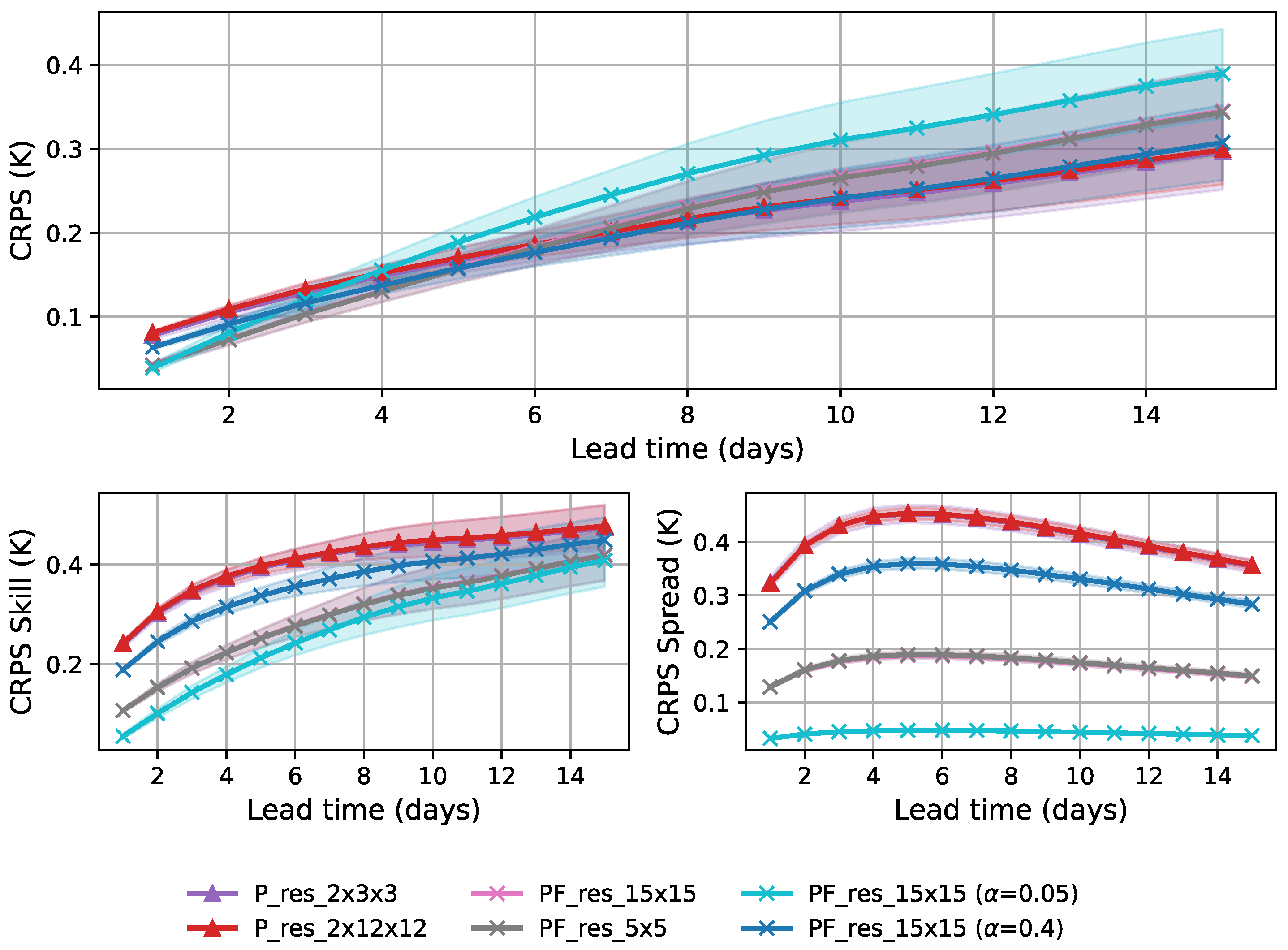
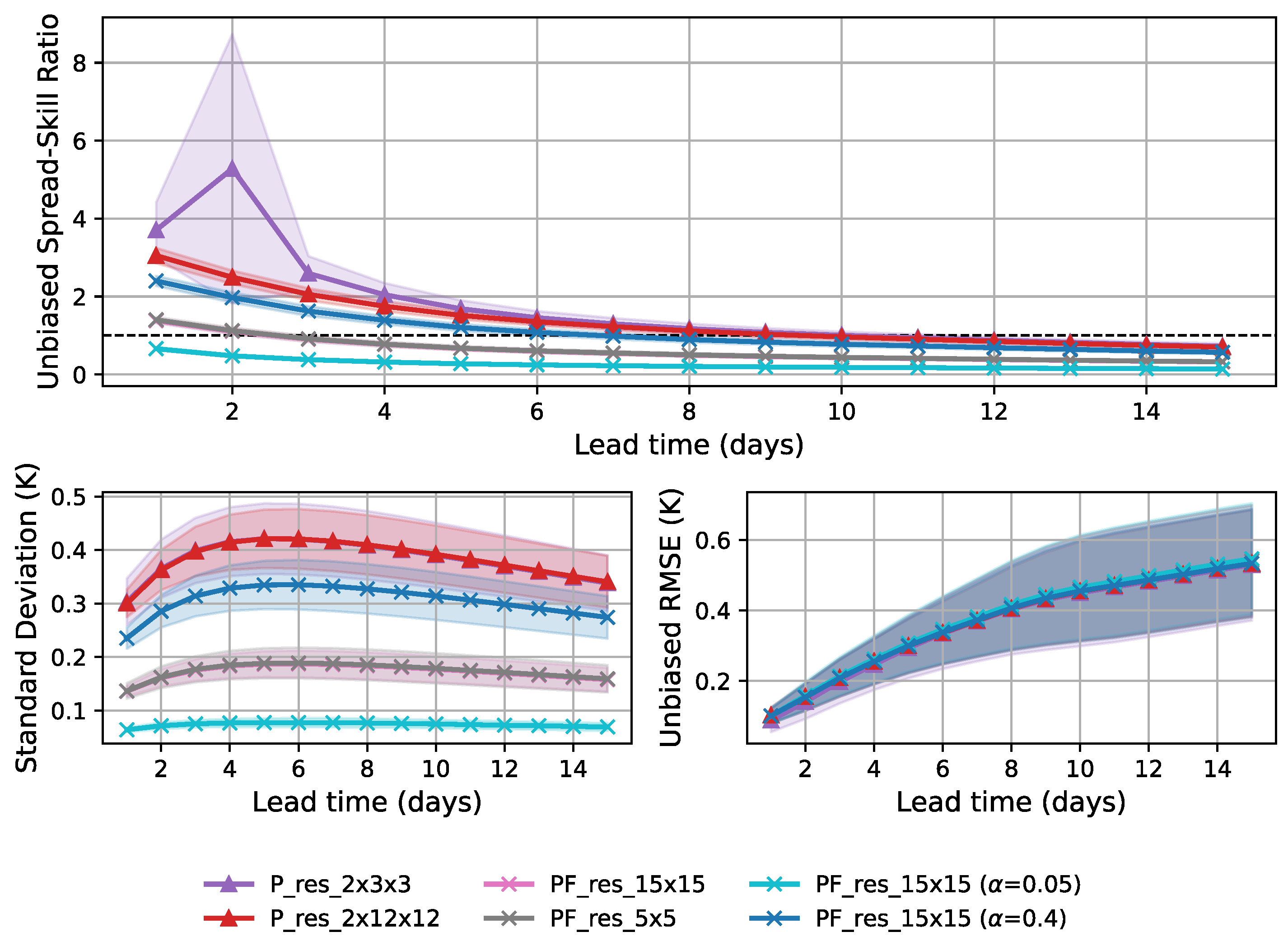
The noise scale parameter is analyzed because it directly controls how strong the random perturbations are. Three values are tested: 0.05, 0.2, and 0.4. The smallest value (0.05) represents a weak-perturbation case that is close to deterministic behavior, while 0.2 corresponds to the baseline used in previous work (Pangu-Weather), and 0.4 represents a strongly perturbed case where random effects become dominant. As shown in Figure 12, the RMSE clearly depends on this parameter. Lower noise values consistently lead to better forecast accuracy. Because of this, all three values are kept for the final evaluation to cover the full range of model behavior under different noise strengths. The selected fractal Perlin configurations are summarized in

Table 5. Fractal Perlin noise configurations used during the tests. The IDs correspond to: (A) PF_res_15x15; (B) PF_res_5x5; (C) PF_res_15x15 ($\alpha$ = 0.05); and (D) PF_res_15x15 ($\alpha$ = 0.4).

ID	Resolution	Repeatable	Persistence	Octaves	Scale	Lacunarity
A	(15, 15)	(F, T)	0.5	3	0.2	2.0
B	(5, 5)	(F, T)	0.5	3	0.2	2.0
C	(15, 15)	(F, T)	0.5	3	0.05	2.0
D	(15, 15)	(F, T)	0.5	3	0.4	2.0

.

All experiments were conducted using an ensemble-based approach. Unless otherwise specified, the default ensemble size was 5 members, each corresponding to a different random realization of the noise. Preliminary tests were first performed using 29 randomly selected initialization dates from the test dataset, matching those used in the noise analysis stage. This stage was used to assess the relative performance of different noise configurations under multiple initial conditions and to discard clearly underperforming candidates, including probabilistic metrics.

To characterize variability, results are reported using empirical 95% confidence intervals computed over evaluation metrics across initialization dates and ensemble members, providing an estimate of performance dispersion under stochastic initialization. No formal statistical significance testing is performed. Therefore, comparisons between configurations are interpreted in terms of relative performance trends and observed variability rather than strict statistical significance.

The configurations selected from this preliminary analysis were then evaluated in a full test setting spanning two years, starting on 1 January 2022. This final evaluation uses continuous forecasts initialized throughout the entire test period, ensuring that results reflect performance across a wide range of meteorological conditions rather than a limited set of initial states.

5. Results

In this section, we compare ensemble prediction with the deterministic forecast. Then, we analyze the differences observed in preliminary experiments using Gaussian and Perlin noise, emphasizing how specific noise parameters influence performance when initial conditions are perturbed.

Table 6. RMSE absolute values and relative increase (%) over different lead times for each noise configuration, with respect to the deterministic model without noise.

Configuration	1 Day	5 Days	15 Days
Deterministic (ref)	0.109 (–)	0.308 (–)	0.586 (–)
Gaussian (${\sigma }^2=0.01$)	0.109 (+0.55%)	0.308 (+0.03%)	0.586 (+0.00%)
Gaussian (${\sigma }^2=0.1$)	0.140 (+28.96%)	0.325 (+5.36%)	0.588 (+0.43%)
PF_res_15x15 ($\alpha =0.05$)	0.110 (+1.56%)	0.309 (+0.16%)	0.586 (+0.02%)
P_res_2x12x12	0.178 (+64.01%)	0.357 (+15.90%)	0.595 (+1.62%)
P_res_2x3x3	0.175 (+61.17%)	0.354 (+14.83%)	0.594 (+1.47%)

reports the RMSE averaged over 1, 5, and 15 days, relative to the deterministic forecast without noise. None of the ensemble configurations consistently outperforms the deterministic model across all horizons, which is expected given that the model was trained under deterministic conditions.

RMSE increases with forecast horizon due to the autoregressive formulation. Ensemble predictions also exhibit higher RMSE at short lead times because the input observations are explicitly perturbed. The largest initial degradations are observed for P_res_2x12x12, P_res_2x3x3, and Gaussian ($\mu =0$, $\sigma =0.1$), reflecting their higher input variability. However, this effect decreases with lead time, and performance converges toward stable values by the final forecast day.

Overall, these results indicate that introducing diversity in the initial conditions helps compensate for forecast errors and promotes exploration of alternative future states, which becomes increasingly important as uncertainty grows in autoregressive predictions. The primary objective of this work was not to improve deterministic accuracy, but to evaluate how different ensemble strategies and input perturbations impact uncertainty characterization.

Figure 13 shows the bias on prediction day 1 for different members of the ensemble and their mean value. The members show greater variability, while the mean of the set is more accurate.

5.1. Comparison of Gaussian Noise Configurations

Table 7. Mean CRPS (SST) for Gaussian noise configurations across lead-time ranges.

Noise Type	1–2d	3–4d	5–6d	7–8d	9–10d	11–12d	13–14d	15–16d
Gaussian ($\mu$ = 0, $\sigma$ = 0.1)	0.064	0.117	0.164	0.206	0.243	0.271	0.302	0.325
Gaussian ($\mu$ = 0, $\sigma$ = 0.05)	0.055	0.120	0.178	0.229	0.271	0.302	0.336	0.360
Gaussian ($\mu$ = 0, $\sigma$ = 0.01)	0.064	0.145	0.212	0.266	0.310	0.341	0.374	0.397

summarizes the mean CRPS for the different Gaussian noise configurations across lead-time ranges.

Figure 14 shows the CRPS (10) and its components, CRPS skill (7) and CRPS spread (8), for the selected Gaussian noise configurations. Values closer to zero indicate better performance of the set, as they reflect a balance between accuracy (low error of the predicted distribution) and adequate dispersion among the predictions of the set, which favors prediction sets that explore more alternatives with controlled error.

In this configuration, the CRPS is higher at the beginning of the forecast horizon when the first two entries correspond to noisy initial states. The figure shows that the CRPS skill curve reflects greater disagreement with actual observations in the early steps. Although the contribution of the CRPS spread helps to mitigate the error, it is not sufficient to achieve the values obtained with lower noise levels. In the latter cases, the lower disturbance of the initial conditions results in better performance in the first days of the forecast.

However, these configurations show a change in trend over the time horizon, reaching their worst performance at the end. This can be understood by analyzing the CRPS skill graph, where the differences in error between the configurations are minimal at the end of the time horizon. As their dispersion (CRPS spread) is lower, these errors are not corrected adequately. Therefore, although the dispersion between the members decreases slightly from the sixth day onwards, the model with the highest noise ends up being the one that best represents the predicted distribution compared to the actual observations.

Table 8. Mean spread–skill ratio (unbiased, SST) for Gaussian noise configurations across lead-time ranges.

Noise Type	1–2d	3–4d	5–6d	7–8d	9–10d	11–12d	13–14d	15–16d
Gaussian ($\mu$ = 0, $\sigma$ = 0.1)	1.638	1.129	0.857	0.705	0.603	0.533	0.470	0.430
Gaussian ($\mu$ = 0, $\sigma$ = 0.05)	0.995	0.646	0.486	0.402	0.346	0.309	0.276	0.255
Gaussian ($\mu$ = 0, $\sigma$ = 0.01)	0.418	0.260	0.195	0.162	0.141	0.127	0.114	0.106

summarizes the mean unbiased spread–skill ratio for the different Gaussian noise configurations across lead-time ranges.

Figure 15 depicts the evolution of the unbiased spread–skill ratio (13) and its components: the standard deviation (11) and the unbiased RMSE. The horizontal line at value 1 on the y-axis represents the reference threshold. This would be the case when the dispersion of the predictions of the set with respect to their mean can completely explain the errors of that mean, indicating perfect calibration.

In this case, the configuration with standard deviation equal to 0.01 presents a subdispersed behavior throughout the entire prediction horizon, with insufficient dispersion with respect to the error committed by its mean. This can be verified by comparing the graph of standard deviation with respect to RMSE, where it is always a lower value. The other two configurations are overdispersed at the beginning, with greater dispersion with respect to their mean. However, a common pattern is detected in the evolution of the spread–skill ratios, as they begin to stabilize from the sixth day onwards. This is consistent with the fact that the standard deviation of the sets grows until day 6, followed by a progressive decline. Furthermore, at this point it is also detected that the RMSE exceeds the standard deviation, which explains the coefficient of less than one in the case of a standard deviation equal to 0.1. Therefore, although all configurations end up being underdispersed, it can be deduced that with a slightly larger but controlled disturbance, it would be possible to achieve a calibration of the set close to one at the end.

5.2. Comparison of Perlin Noise Configurations

Table 9. Mean CRPS (SST) for Perlin noise configurations across lead-time ranges.

Noise Type	1–2d	3–4d	5–6d	7–8d	9–10d	11–12d	13–14d	15–16d
(A)	0.092	0.139	0.176	0.207	0.232	0.253	0.277	0.296
(B)	0.095	0.143	0.178	0.209	0.236	0.257	0.280	0.299
(C)	0.058	0.117	0.171	0.219	0.259	0.289	0.322	0.345
(D)	0.058	0.117	0.169	0.217	0.257	0.287	0.320	0.344
(E)	0.060	0.138	0.204	0.258	0.302	0.333	0.366	0.390
(F)	0.077	0.127	0.167	0.203	0.235	0.258	0.286	0.307

Legend: (A) P_res_2x3x3; (B)  P_res_2x12x12; (C) PF_res_15x15; (D) PF_res_5x5; (E) PF_res_15x15 ($\alpha$ = 0.05); (F) PF_res_15x15 ($\alpha$ = 0.4).

summarizes the mean CRPS for the different Perlin noise configurations across lead-time ranges.

The Perlin noise results corresponding to the first days of prediction for CRPS are shown in Figure 16. The configurations with base Perlin noise (P_res_2x3x3 and P_res_2x12x12) show lower initial performance. However, these experiments end up being the best at the end of the time horizon compared to the fractal Perlin configurations, following a similar trend to Gaussian noise ($\mu$ = 0, ${\sigma }^2$ = 0.1). The configurations with Perlin fractal noise start with initial CRPS values close to the ideal, but their performance deteriorates over time.

One of the differences between the two groups is the complexity of the noise. Perlin fractal noise uses multiple iterations to refine the pattern, each with a higher resolution. However, the influence of these last octaves is minor, so only fine details are added. In contrast, base Perlin noise is simpler, as it generates the noise only once with the input resolution. Furthermore, fractal Perlin noise configurations incorporate a noise scalability factor, represented by $\alpha$, which is applied to the output to attenuate its impact.

The magnitude of the Perlin fractal noise with a scalability of 0.4 is comparable to the base Perlin noise. However, the dispersion between members is lower in this case, despite using a similar noise intensity. This suggests that fractal Perlin noise is not beneficial due to noise refinement through octaves, which generates complex spatial patterns with less structural coherence, thus affecting uncertainty.

Table 10. Mean spread–skill ratio (unbiased, SST) for Perlin noise configurations across lead-time ranges.

Noise Type	1–2d	3–4d	5–6d	7–8d	9–10d	11–12d	13–14d	15–16d
(A)	4.492	2.319	1.571	1.238	1.041	0.909	0.795	0.723
(B)	2.772	1.903	1.434	1.174	0.999	0.879	0.770	0.703
(C)	1.243	0.838	0.633	0.521	0.447	0.396	0.351	0.322
(D)	1.261	0.846	0.640	0.528	0.452	0.401	0.355	0.327
(E)	0.569	0.349	0.259	0.215	0.187	0.168	0.152	0.141
(F)	2.187	1.507	1.143	0.940	0.803	0.709	0.623	0.569

Legend: (A) P_res_2x3x3; (B) P_res_2x12x12; (C) PF_res_15x15; (D) PF_res_5x5; (E) PF_res_15x15 ($\alpha$ = 0.05); (F) PF_res_15x15 ($\alpha$ = 0.4).

summarizes the mean unbiased spread–skill ratio for the different Perlin noise configurations across lead-time ranges.

Regarding the unbiased spread–skill ratio, Figure 17 shows that the basic Perlin configurations stand out once again. Although they exhibit overdispersion over the time horizon, on the 9th day of prediction they reach a value close to one, indicating an almost perfect calibration. Furthermore, it can be seen that in all sets, the standard deviation begins to decrease from the sixth day, as was already the case with Gaussian noise. This decrease, together with a less pronounced increase in unbiased RMSE, causes the spread–skill ratio to stabilize. On the contrary, due to the low intensity of the initial noise, most fractal Perlin configurations end up being underdispersed during most of the prediction period.

Regarding the RMSE in the unified predictions,

Table 11. Mean RMSE (SST) for Perlin noise configurations across lead-time ranges.

Noise Type	1–2d	3–4d	5–6d	7–8d	9–10d	11–12d	13–14d	15–16d
(A)	0.197	0.289	0.362	0.418	0.457	0.485	0.513	0.534
(B)	0.206	0.299	0.369	0.424	0.466	0.492	0.520	0.540
(C)	0.154	0.250	0.331	0.394	0.443	0.474	0.507	0.530
(D)	0.154	0.250	0.329	0.393	0.441	0.473	0.505	0.528
(E)	0.140	0.241	0.323	0.389	0.438	0.471	0.505	0.528
(F)	0.184	0.276	0.351	0.409	0.453	0.481	0.510	0.532

Legend: (A) P_res_2x3x3; (B) P_res_2x12x12; (C) PF_res_15x15; (D) PF_res_5x5; (E) PF_res_15x15 ($\alpha$ = 0.05); (F) PF_res_15x15 ($\alpha$ = 0.4).

shows that higher noise levels tend to result in worse performance across the forecast horizon. However, as observed in the previous noise selection phase, differences between Perlin configurations are generally modest, with most approaches converging to similar error values at longer lead times.

5.3. Comparison Between Types of Noise

The most promising noises underwent an additional test in which predictions were made starting on the same days as the previous ones, but with the set size increased to 10. However, in this case, the results did not show significant differences, with minimal changes relative to prior trends. In the final evaluation, the noises with the best performance according to the previous metrics for each group were selected, along with one representative of each type of noise with the worst results for comparison purposes.

Table 12. Mean CRPS (SST) for Perlin noise and Gaussian configurations across lead-time ranges.

Noise Type	1–2d	3–4d	5–6d	7–8d	9–10d	11–12d	13–14d	15–16d
A	0.093	0.142	0.183	0.221	0.257	0.292	0.325	0.349
B	0.094	0.143	0.184	0.221	0.257	0.292	0.325	0.349
C	0.058	0.142	0.216	0.279	0.333	0.380	0.420	0.447
D	0.062	0.118	0.172	0.223	0.270	0.313	0.353	0.380
E	0.062	0.149	0.224	0.287	0.342	0.388	0.428	0.454

Legend: (A) P_res_2x3x3; (B) P_res_2x12x12; (C) PF_res_15x15 ($\alpha$ = 0.05); (D) Gaussian ($\mu$ = 0, ${\sigma }^2$ = 0.1); (E) Gaussian ($\mu$ = 0, ${\sigma }^2$ = 0.01).

,

Table 13. Mean Spread–skill ratio (unbiased, SST) for Perlin noise and Gaussian configurations across lead-time ranges.

Noise Type	1–2d	3–4d	5–6d	7–8d	9–10d	11–12d	13–14d	15–16d
A	3.484	2.124	1.464	1.156	0.964	0.831	0.729	0.666
B	2.863	1.911	1.425	1.149	0.968	0.838	0.738	0.676
C	0.579	0.348	0.256	0.208	0.178	0.158	0.142	0.133
D	1.676	1.132	0.846	0.684	0.578	0.502	0.444	0.408
E	0.427	0.261	0.193	0.157	0.135	0.119	0.108	0.101

Legend: (A) P_res_2x3x3; (B) P_res_2x12x12; (C) PF_res_15x15 ($\alpha$ = 0.05); (D) Gaussian ($\mu$ = 0, ${\sigma }^2$ = 0.1); (E) Gaussian ($\mu$ = 0, ${\sigma }^2$ = 0.01).

and

Table 14. Mean RMSE (unbiased, SST) for Perlin noise and Gaussian configurations across lead-time ranges.

Noise Type	1–2d	3–4d	5–6d	7–8d	9–10d	11–12d	13–14d	15–16d
A	0.122	0.219	0.311	0.386	0.447	0.498	0.541	0.570
B	0.123	0.225	0.315	0.388	0.449	0.500	0.542	0.570
C	0.124	0.230	0.322	0.398	0.460	0.512	0.555	0.584
D	0.122	0.225	0.317	0.393	0.455	0.506	0.549	0.577
E	0.127	0.233	0.324	0.400	0.462	0.513	0.556	0.585

Legend: (A) P_res_2x3x3; (B) P_res_2x12x12; (C) PF_res_15x15 ($\alpha$ = 0.05); (D) Gaussian ($\mu$ = 0, ${\sigma }^2$ = 0.1); (E) Gaussian ($\mu$ = 0, ${\sigma }^2$ = 0.01).

summarize the mean CRPS, unbiased spread–skill ratio, and RMSE, respectively, for Perlin noise and Gaussian configurations across lead-time ranges.

Figure 18 is consistent with the trends observed in the preliminary experiments, where noise intensity appears important for ensuring sufficient ensemble diversity (e.g., for a Gaussian standard deviation of 0.1). Unlike the preliminary analysis based on single initialization dates, the results shown here are obtained by averaging the metrics over all prediction start dates in the test period (2022–2023), providing a broader assessment. Under this evaluation, overall performance decreases, and the differences between configurations become smaller. Nevertheless, Perlin noise still shows better performance than the Gaussian noise configurations.

Despite the difference in the statistical distribution of noise between the configurations of both groups, the noise intensities are similar in those with comparable performance (e.g., Gaussian noise $\sigma =0.1$ and Perlin base P_res_12x12). This suggests that the models benefit from initial perturbations that combine adequate noise intensity with some spatial structure.

6. Discussion

While deterministic error remains comparable to the single-model forecast, the predictions reveal important patterns in ensemble performance and uncertainty, providing a basis for further investigation.

The analysis of the initial perturbations shows differences depending on their structure and intensity. Perturbations generated with moderate noise and structured spatial patterns (such as Perlin noise) appear more effective than those generated with unstructured noise (e.g., Gaussian noise), which does not incorporate explicit spatial structure. Furthermore, iterating over spatial noise patterns by introducing finer-scale details in successive steps (as in Perlin fractal noise) did not lead to noticeable improvements.

A limitation of this study is that, although the noise configurations are explored through a structured sensitivity analysis, the parameter space is not exhaustively sampled in a global sense. Instead, we focus on a set of representative configurations selected from predefined parameter ranges in order to enable controlled comparisons of different perturbation structures under computational constraints. While this ensures a systematic and interpretable analysis, it may still omit configurations that could further improve performance or reveal additional behaviors.

In addition to these findings, it is important to consider the characteristics of the base model when interpreting the results. The model is relatively simple, both in terms of the number of variables and the training procedure, and it was trained deterministically. Despite this, some predictions obtained by perturbing the initial state perform similarly to the original, unperturbed model in this specific case. This suggests that adding small changes at inference time can introduce some forecast variability without changing the training process. However, more work is needed to understand whether this result would hold for more complex models or datasets. Although ensemble predictions tend to perform worse at early stages, differences between individual predictions seem to balance out over time, leading to an average result similar to the deterministic model.

The current model is limited by the use of the SST and surface winds, which restricts its ability to capture complex oceanographic processes, such as coastal upwelling, mesoscale circulation, or vertical mixing. Incorporating additional physical variables in future work could improve the dynamical realism of forecasts and allow ensemble perturbations to better represent variability from these processes.

Future work could explore incorporating CMEMS error estimates to scale ensemble perturbations or weight training samples. Doing so would allow the ensemble to more accurately reflect observational uncertainty, particularly in regions with strong variability such as the Canary Islands upwelling region.

It is important to note that the model was trained using a single-step objective (T = 1) and extended to 15-day forecasts via autoregressive rollout during testing. This discrepancy between the training and inference horizons is a known limitation of one-step training and can contribute to error accumulation at longer lead times. The primary goal of this work is not to optimize the forecasting model itself, but to evaluate how ensemble perturbation strategies influence prediction diversity on a fixed baseline. Incorporating multi-step rollouts during training could improve long-term stability and represents a potential direction for future work.

This study identified several issues for further research beyond the exclusive perturbation of initial oceanographic data during inference. One possible direction is to train the model with autoregressive steps, which could improve the accuracy of long-term predictions. In this work, noise was added exclusively to the initial oceanographic states of the model. Considering that only one variable was used, this diversity may not be sufficient to capture complex phenomena such as coastal upwelling, which probably requires a greater number of variables to explain adequately. This scenario would also allow us to validate the conclusions drawn in this work regarding the types of noise that are most beneficial for creating larger-scale prediction sets.

Similarly, other types of ensemble learning techniques could be used for comparison, including the use of lagged predictions, the perturbation of initial forcing states, or the modification of the model parameters. As one of the advantages of ensemble learning techniques is their great flexibility, future work could focus on introducing diversity in the training phase rather than inference, provided the necessary computational resources are available. Although no significant improvements were obtained in this work by increasing the number of ensemble members, this is likely due to the small number of predictions used, conditioned by computational limitations. This deficiency was evident in the analysis of the unbiased RMSE, where in several scenarios the results changed dramatically.

Therefore, this work aims to serve as an initial reference in the study of the types of noise applied during the inference phase as a mechanism for introducing diversity into prediction sets. However, as discussed throughout this section, the possibilities for configuring and incorporating diversity in this type of technique are extensive. As a result, future lines of research could focus on improving the results obtained in this work using the same techniques or exploring any of the other options mentioned.