Article

A Taxonomy of Generative Models with a Focus on Diffusion Models and Denoising Techniques

1
Washkewicz College of Engineering, Cleveland State University, Cleveland, OH 44115, USA
2
Department of Computer Science, Kent State University, Kent, OH 44242, USA
3
Khoury College of Computer Sciences, Northeastern University, Boston, MA 02115, USA
4
Khoury College of Computer Sciences, Roux Institute at Northeastern University, Portland, ME 04101, USA
*
Author to whom correspondence should be addressed.
Electronics 2026, 15(6), 1293; https://doi.org/10.3390/electronics15061293
Submission received: 15 February 2026 / Revised: 16 March 2026 / Accepted: 18 March 2026 / Published: 19 March 2026
(This article belongs to the Special Issue Autonomous Intelligence: Concepts and Applications of Agentic AI)

Abstract

Diffusion models have emerged as a powerful class of generative models, demonstrating impressive results across visual domains such as image and video synthesis. This survey provides a comprehensive taxonomy of generative models, with a particular focus on diffusion models and their applications in enhancing visual fidelity for text-to-image and text-to-video generation. We discuss the theoretical foundations of diffusion models, including their formulation through stochastic differential equations, and analyze the forward noising and reverse denoising processes that enable stable training and high-quality generation. The survey further categorizes diffusion architectures, including pixel-space and latent-space models, and examines their design choices, training strategies, and trade-offs across different resolution regimes. In addition, we review noise characteristics in real-world imaging domains and discuss their implications for diffusion-based models. Denoising strategies are analyzed by distinguishing between in-model denoising mechanisms and external denoising techniques used in preprocessing and post-processing pipelines. The survey also summarizes commonly used datasets and evaluation metrics for generative modeling, providing a practical perspective on benchmarking and model comparison. Finally, we discuss current challenges, including computational efficiency, scalability, and robustness to diverse noise distributions, and outline potential directions for future research. This survey aims to provide a structured reference for understanding diffusion models and their applications in visual generation tasks.

1. Introduction

Diffusion models have rapidly gained prominence as a powerful class of generative models, demonstrating significant potential across diverse domains, from image synthesis and video generation to molecular design and audio processing. Their success stems from their ability to simulate complex data distributions, which has enabled remarkable advances in producing realistic and high-fidelity media content. With the growing availability of data and computational resources, diffusion models are increasingly being applied in various fields to generate high-quality images, videos, and other data representations from simple prompts or latent inputs. For instance, text-to-image diffusion models have revolutionized the creative arts and design industries by generating photorealistic and stylistic images from text descriptions, transforming how artists and content creators envision and produce visual assets. In medical imaging, diffusion models are being explored for enhanced diagnostic tools, aiming to reconstruct high-resolution images from noisy or incomplete scans, thereby improving accuracy and accessibility of medical care. Similarly, diffusion models are making strides in environmental science and remote sensing, where they enable improved data generation for predictive modeling and enhanced satellite imagery interpretation. One of the core strengths of diffusion models lies in their unique noising and denoising mechanisms. These processes, based on principles from stochastic differential equations, involve systematically introducing noise into data and learning to reverse this process to reconstruct or generate new data samples. This sequence of steps allows diffusion models to explore complex data manifolds and accurately approximate underlying data distributions, enhancing their capacity for generating realistic outputs. In image and video generation, the noising process helps diffusion models learn the intricate details of visual data, making them highly effective in producing nuanced textures, colors, and shapes. Conversely, the denoising process plays a pivotal role in reconstructing high-quality outputs, as it allows the model to iteratively refine the data, removing unwanted noise and amplifying relevant features to achieve visual fidelity. These techniques have shown impressive results in reducing artifacts and enhancing the clarity of generated media, proving particularly beneficial in applications where high-resolution and detailed outputs are critical.
Despite the advancements, diffusion models face challenges, particularly in terms of computational efficiency and robustness. The iterative noising and denoising processes require substantial computational power, often demanding extended training times and significant energy resources, which can limit their applicability in real-time or large-scale deployments. Moreover, diffusion models must contend with maintaining temporal consistency in video generation, as even minor inconsistencies can disrupt the flow of generated frames, reducing the realism of the output. Addressing these challenges is crucial for further advancing the field, making it essential to explore innovative architectures, optimized training methods, and resource-efficient techniques that can scale diffusion models for broader and more sustainable use.
This survey aims to provide a comprehensive taxonomy of generative models, with a particular focus on diffusion models and their noising and denoising techniques for enhancing visual fidelity in text-to-image and text-to-video applications. By delving into the mathematical foundations, architectures, and training methodologies of diffusion models, this survey seeks to bridge the gap in the existing literature, where detailed classifications and comparisons of these models are often lacking.
While several recent surveys have reviewed diffusion models from specific perspectives, such as architectural design or application domains, most adopt a single axis of categorization (e.g., grouping models by architecture alone or by application area). In contrast, this survey introduces a five dimensional classification system that simultaneously organizes diffusion models along representation space, forward process formulation, reverse parameterization, sampling strategy, and conditioning mechanism. This multi axis perspective enables a more granular comparison of models that may share certain design choices while differing in others, thereby revealing structural relationships that are not apparent from single axis taxonomies. To our knowledge, this is the first survey to provide such a unified, orthogonal classification framework for diffusion models, offering both theoretical clarity and practical guidance for model selection.
The contributions of this paper are as follows:
  • Position diffusion models within a broader taxonomy of generative models, including explicit likelihood-based models, variational or score-based models, and implicit models.
  • Provide a structured taxonomy of diffusion models based on key design dimensions, including representation space, forward process formulation, reverse parameterization, sampling strategy, and conditioning mechanisms.
  • Analyze architectural variations in diffusion models, including pixel-space, latent-space, and transformer-based approaches.
  • Discuss noise characteristics in real-world imaging domains, and their impact on diffusion-based generative modeling.
  • Summarize commonly used datasets and evaluation metrics for diffusion models, covering pixel-level, perceptual, and distribution-based measures.
  • Highlight practical trade-offs across models, including computational cost, memory requirements, sampling efficiency, and output fidelity across different resolution regimes.
By consolidating architectural, theoretical, and evaluation perspectives, this overview is intended as a reference for researchers and practitioners working with diffusion-based visual generation systems. The remainder of this paper is organized as follows: Section 2 presents a taxonomy of generative models. Section 3 introduces the formulation of diffusion models, including forward and reverse processes. Section 4 discusses noise characteristics in imaging and video domains. Section 5 reviews denoising strategies in diffusion models. Section 6 summarizes commonly used datasets. Section 7 presents evaluation metrics. Section 8 provides a comparative analysis of representative models. Finally, Section 9 concludes the paper and outlines future directions.

2. Taxonomy by Architecture Generative Models for Image and Video Generation

Generative models aim to learn the underlying probability distribution of observed data so that new samples can be generated that resemble the training data. Formally, given data samples x p data ( x ) , the goal of a generative model is to learn a model distribution p θ ( x ) that approximates the true data distribution.
In likelihood-based modeling, training typically involves maximizing the log-likelihood l o g   p θ ( x ) , which is equivalent to minimizing the divergence between the learned distribution and the true data distribution under standard assumptions. This probabilistic perspective provides a principled statistical foundation for generative modeling.
Different generative paradigms vary in how they represent and optimize this distribution. Some models define and evaluate likelihoods directly, others optimize approximations to likelihood, and some avoid explicit likelihood modeling altogether
From this perspective, generative models can be broadly categorized into three groups:
  • Explicit Density Models;
  • Variational/Score-Based Density Models;
  • Implicit Models.
This taxonomy (Figure 1) provides a principled foundation for positioning diffusion models within the broader generative landscape and clarifies how different modeling assumptions lead to distinct training objectives, computational trade-offs, and sampling procedures.

2.1. Explicit Density Models

Explicit density models are generative models that define a tractable probability density function p θ ( x ) over the data space. In these models, the likelihood of an observed sample can be computed exactly and optimized directly via maximum likelihood estimation (MLE). Formally, training consists of maximizing:
L ( θ ) = E x d a t a [ l o g   p θ ( x ) ]
Because the likelihood is explicitly defined and computable, these models provide strong statistical interpretability and stable optimization objectives. A key characteristic of explicit density models is that they either: Factorize the joint distribution into conditionals that are easy to evaluate or Apply invertible transformations with tractable Jacobian determinants. This category primarily includes autoregressive models and flow-based models.

2.1.1. Autoregressive Models

Autoregressive (AR) models define joint distribution over data as a product of conditional probabilities using the chain rule of probability:
p θ ( x ) = i = 1 D p θ   x i   x i )
here x i denotes all variables preceding x i .
In image modeling, this corresponds to generating pixels sequentially; in language modeling, tokens are generated one at a time. Examples include PixelRNN [1], and PixelCNN [2]. These models are widely used in text, audio, and image generation, particularly where spatial or temporal dependencies are critical. Because each conditional distribution is explicitly modeled, the likelihood can be computed exactly. This makes AR models statistically well-founded and straightforward to train via maximum likelihood.
However, sampling is inherently sequential. Generation requires one forward pass per dimension, leading to high computational cost for high-resolution images or long sequences. This limits their scalability in large visual domains.

2.1.2. Flow-Based Models

Flow-based models learn an invertible transformation between the data space and a simple latent distribution (Figure 2), typically a multivariate Gaussian. Unlike autoregressive models, they enable exact likelihood evaluation while maintaining a bidirectional mapping between data and latent variables. Let:
z = f θ ( x )
where x X is a data sample, z Z is a latent variable drawn from a simple prior distribution (e.g., N ( 0 , I ) ), and f θ is an invertible transformation parameterized by neural network parameters θ . Because f θ is invertible, reconstruction is obtained via
x = f θ 1 ( z )
The exact data likelihood is computed using the change-of-variables formula:
log p θ x = log p z   l o g d e t f θ x
Here, the second term represents the log-determinant of the Jacobian of the transformation. Flow architectures such as coupling layers and invertible 1 × 1 convolutions are specifically designed to ensure that this Jacobian determinant is tractable, allowing exact likelihood computation during training. Notable flow-based models, such as NICE [3], RealNVP [4] and Glow [5], allow for reversible data transformations, making them suitable for image generation and tasks requiring precise control over generated data.

2.2. Variational and Score-Based Density Models

Unlike explicit density models, which compute tractable likelihoods directly, this class models the data distribution by optimizing either a variational lower bound or a score-matching objective. In these approaches, the likelihood is not always computed in closed form but is approximated through auxiliary objectives that remain probabilistically grounded.

2.2.1. Variational Autoencoders (VAEs)

Variational Autoencoders (VAEs) model the data distribution using latent variables and optimize a variational lower bound on the log-likelihood [6,7,8,9,10,11].
Given an observed data x , a latent variable z is introduced with prior p ( z ) . The marginal likelihood is defined as:
p θ ( x ) = p θ ( x z ) p ( z )   d z
Because this integral is generally intractable, VAEs introduce an approximate posterior distribution q ϕ ( z x ) and maximize the Evidence Lower Bound (ELBO):
l o g   p θ ( x ) E q ϕ ( z x ) [ l o g   p θ ( x z ) ] D K L ( q ϕ ( z x ) p ( z ) )
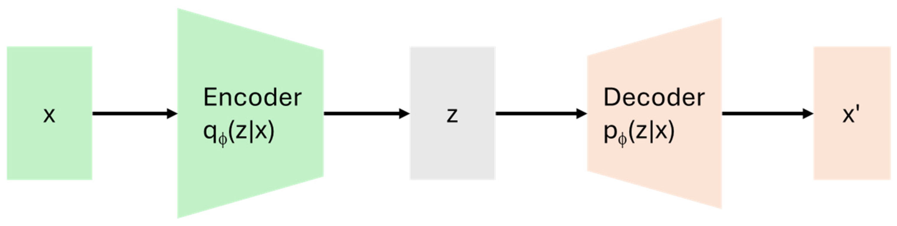
The first term corresponds to the reconstruction objective, while the second term regularizes the approximate posterior toward the prior distribution. This formulation enables stable training while maintaining a probabilistic interpretation. The encoder learns q ϕ ( z x ) , mapping data to a continuous latent space, and the decoder models p θ ( x z ) , enabling reconstruction and generation (Figure 3). VAEs are commonly suitable for tasks such as image reconstruction, latent interpolation, representation learning, and anomaly detection. Notable VAE variants include Conditional VAE (CVAE), Graph Convolutional VAE (GCN-VAE), and Vector Quantized VAE (VQ-VAE). Table 1 discusses the key features of these variants.

2.2.2. Diffusion and Score-Based Models

Diffusion models learn to approximate the data distribution by reversing a gradual noise corruption process. During training, data are progressively perturbed by a predefined forward process. A neural network then learns to invert this process, effectively modeling the score function or a variational objective equivalent to denoising score matching. Score-based generative modeling via stochastic differential equations provides a continuous-time interpretation of diffusion models and unifies discrete diffusion probabilistic models with score-matching frameworks. A detailed discussion of the forward and reverse processes, score-matching interpretation, and sampling formulations is provided in Section 3. Diffusion models have emerged as a dominant paradigm in visual generation due to their stability, scalability, and high sample quality. In this survey, we organize diffusion methods along architectural and formulation axes introduced in the subsequent sections.

2.3. Implicit Models

Implicit generative models do not define or evaluate a tractable likelihood function. Instead of modeling p θ ( x ) explicitly, they learn to generate samples whose distribution matches the data distribution through adversarial or distribution-matching objectives.
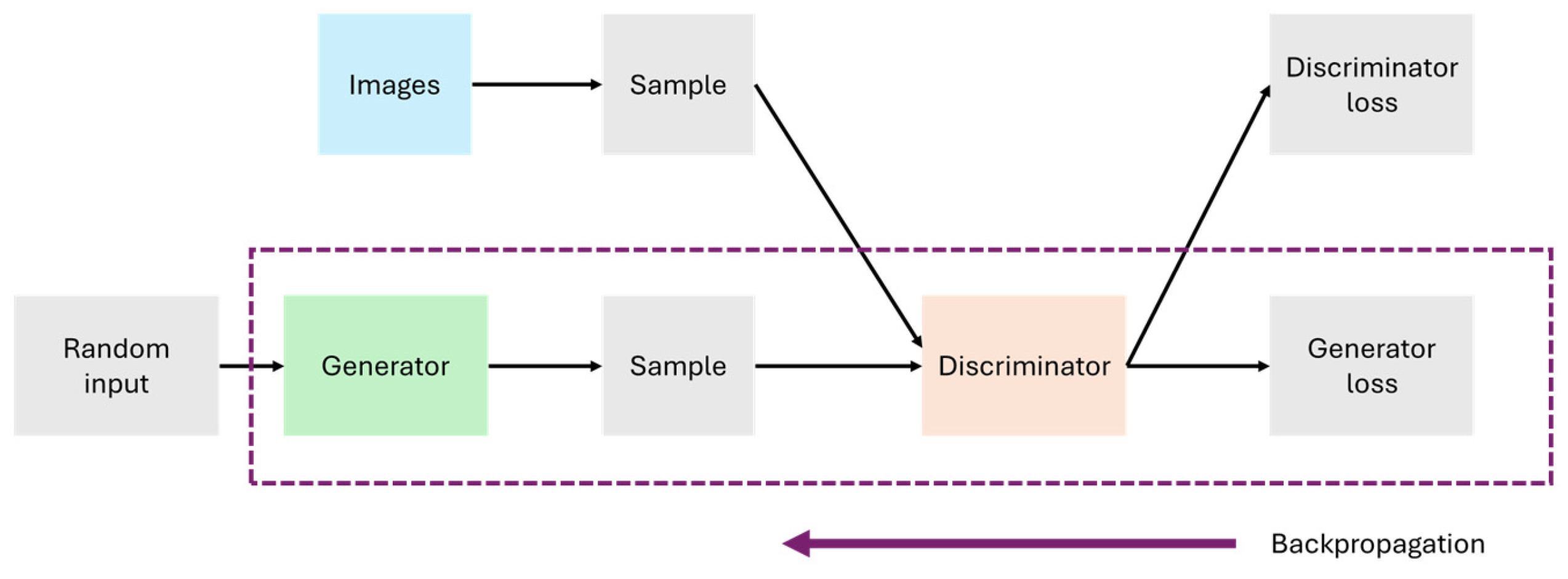
Generative Adversarial Networks (GANs) are the most prominent example of this class [12,13,14]. A GAN consists of two components (Figure 4):
  • A generator G ( z ) , which maps a latent variable z p ( z ) to the data space.
  • A discriminator D ( x ) , which attempts to distinguish real samples from generated ones.
Training is formulated as a minimax objective:
min G   max D   E x p d a t a [ l o g D ( x ) ] + E z p ( z ) [ l o g ( 1 D ( G ( z ) ) ) ]
Rather than maximizing likelihood directly, GANs implicitly minimize a divergence between the model distribution and the data distribution through adversarial learning.
GANs have been widely applied to image synthesis and related generative tasks. Representative variants include StyleGAN, CycleGAN, InfoGAN, MaskGAN, and others. These variants primarily differ in architectural design and training objectives, rather than in their fundamental implicit modeling principle as illustrated in Table 2.
Despite the growing dominance of diffusion models in generative tasks, GANs retain several notable advantages in certain settings. In particular, GANs perform inference through a single forward pass of the generator network, enabling real time image synthesis that is orders of magnitude faster than iterative diffusion sampling. The adversarial training objective also encourages the generator to produce outputs with sharp, realistic details, which can be advantageous for tasks such as super resolution and style transfer where perceptual quality is paramount [12,13].
Moreover, recent work has explored integrating the strengths of both paradigms. For example, Denoising Diffusion GANs [27] combine the stable, multi step denoising framework of diffusion models with adversarial training, using a GAN to model each denoising step as a multimodal conditional distribution rather than a simple Gaussian. This hybrid approach significantly reduces the number of sampling steps required while maintaining high sample quality, effectively addressing one of the primary limitations of pure diffusion models. Such integrations suggest that adversarial and diffusion-based methods are not mutually exclusive but can be combined to leverage the efficiency of GANs and the distributional coverage of diffusion models.

2.4. Comparative Summary of Generative Model Paradigms

To provide a unified perspective on the generative modeling landscape, Table 3 presents a systematic comparison of the four major paradigm families discussed in this survey: Variational Autoencoders (VAEs), Generative Adversarial Networks (GANs), flow-based models, and diffusion models. The comparison spans key dimensions that are relevant to both researchers and practitioners when selecting a generative framework for a given application.
As Table 3 illustrates, diffusion models offer a distinctive balance of training stability, sample quality, and mode coverage, though at the cost of slower sampling. GANs remain competitive in scenarios that demand rapid inference, while VAEs and flow-based models offer complementary strengths in latent representation and exact likelihood computation, respectively. This comparison motivates the detailed taxonomy of diffusion models presented in Section 3, where we further differentiate diffusion approaches along five orthogonal design dimensions.

3. Diffusion Model: Foundations and Taxonomy

3.1. Diffusion Model

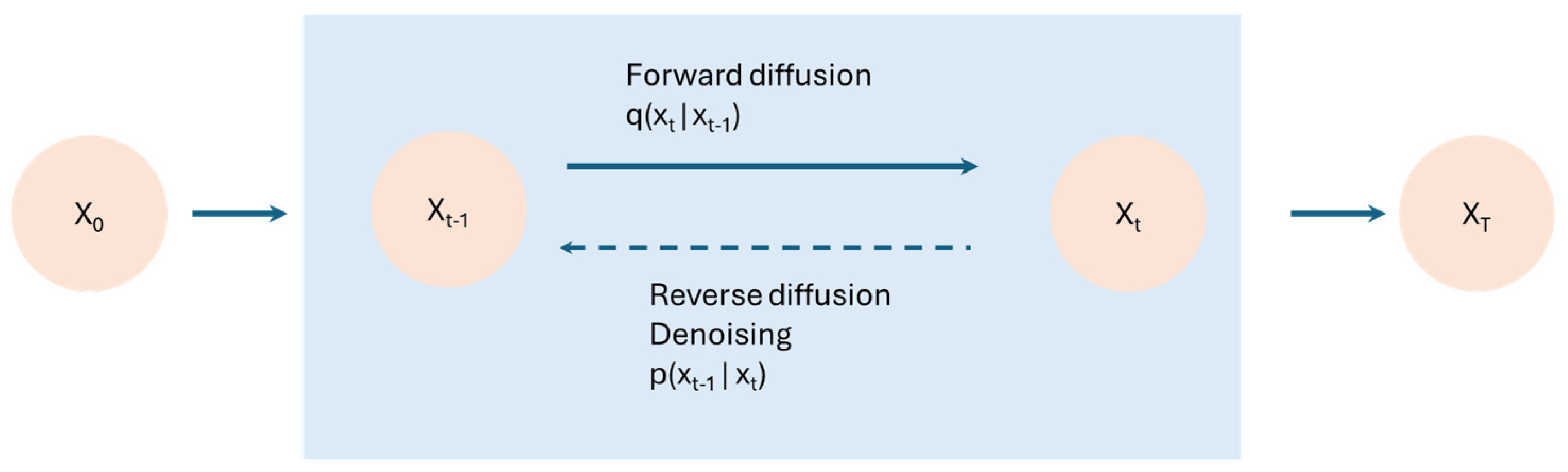
Diffusion models are a class of generative models that approximate the data distribution by reversing a gradual noise corruption process. Starting from a random noise sample, the model generates data through an iterative denoising procedure governed by a learned reverse process (Figure 5).
During training, a forward process progressively perturbs data by adding noise over a sequence of steps. A neural network is then trained to approximate the reverse transformation, enabling the reconstruction of data from noisy inputs. This formulation can be interpreted as learning a sequence of conditional distributions and is closely related to variational inference and score-based modeling approaches. Diffusion models have been widely applied to generative tasks such as image and video synthesis. Representative approaches include Denoising Diffusion Probabilistic Models (DDPM) [28], Stable Diffusion [29], Latent Diffusion Models (LDM) [30], and Text-Guided Diffusion Models [31].

3.1.1. Forward Diffusion Process

The forward diffusion process progressively perturbs data by adding noise over a sequence of discrete time steps. Given an initial data sample x 0 p data ( x ) , the forward process is defined as a Markov chain:
q ( x t x t 1 ) = N ( x t ;   ( 1 β t )   x t 1 , β t I )
where β t ( 0,1 ) is a predefined variance schedule controlling the amount of noise added at each step.
By repeatedly applying this process, the data is gradually transformed into noise:
x 0 x 1 x T
After a sufficient number of steps T , the distribution of x T approaches a standard Gaussian distribution:
x T N ( 0 , I )  
The forward process is fixed and does not involve learnable parameters. It defines the corruption process that the model learns to invert.

3.1.2. Reverse Diffusion Process

The reverse diffusion process aims to reconstruct data by reversing the forward noising process. This is modeled as a sequence of conditional distributions:
p θ ( x t 1 x t )
Each reverse step is typically parameterized as a Gaussian distribution:
p θ ( x t 1 x t ) = N ( x t 1 ; μ θ ( x t , t ) , Σ θ ( x t , t ) )
where a neural network predicts the parameters of the distribution conditioned on the current noisy sample x t and the time step t .
Starting from noise x T N ( 0 , I ) , the model iteratively applies the reverse transitions:
x T x T 1 x 0
to generate a sample from the data distribution.

3.1.3. Training Objective

Training diffusion models can be formulated as maximizing a variational bound on the data likelihood. In practice, this objective is often simplified to a denoising loss.
A common formulation trains the model to predict the noise added during the forward process:
L = E x 0 , ϵ , t ϵ ϵ θ ( x t , t ) 2
where the noisy sample x t is constructed as:
x t = α ¯ t x 0 + 1 α ¯ t ϵ , ϵ N ( 0 , I )
This objective can be interpreted as a form of denoising score matching and is equivalent, under certain assumptions, to optimizing a variational lower bound.

3.2. Diffusion Model Variants

Diffusion models have evolved into several variants that differ in how they represent data, formulate the diffusion process, parameterize the reverse dynamics, and perform sampling. Rather than treating these models as independent architectures, this work organizes them along a set of design dimensions introduced in the following section. Here, we briefly outline representative classes of diffusion models.

3.2.1. Denoising Diffusion Probabilistic Models (DDPM)

Denoising Diffusion Probabilistic Models (DDPM) [28] serve as the foundational framework for modern diffusion models. They rely on a forward process that gradually adds Gaussian noise to the data over a series of timesteps, effectively transforming the data into pure noise. During the reverse process, DDPM learns to sequentially remove the noise at each step to reconstruct the original data. This step-by-step refinement allows DDPMs to generate outputs that are both high-quality and diverse, as depicted Figure 6. The model leverages variational inference to optimize the reverse process and has demonstrated exceptional capabilities in tasks such as image generation, inpainting, and super-resolution.

3.2.2. Latent Diffusion Models

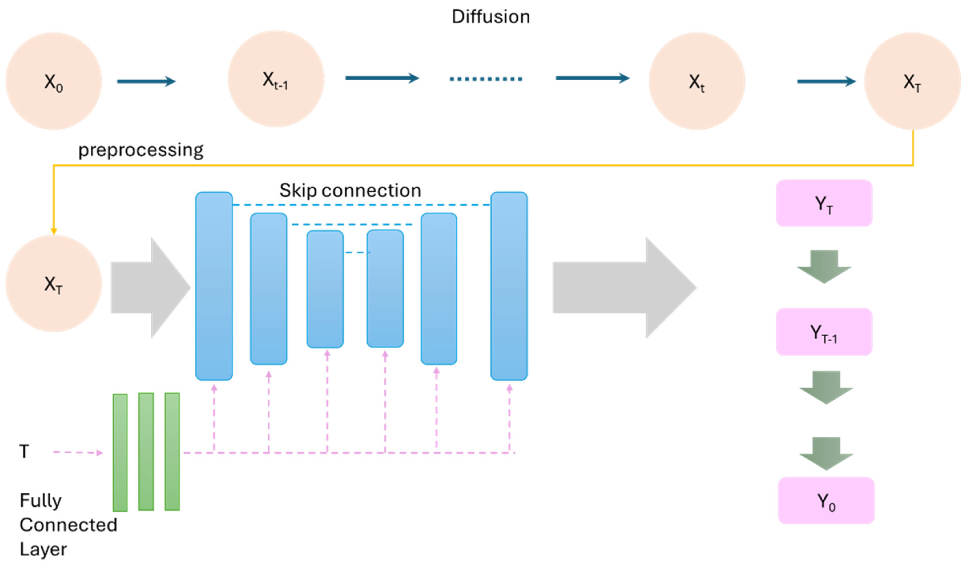
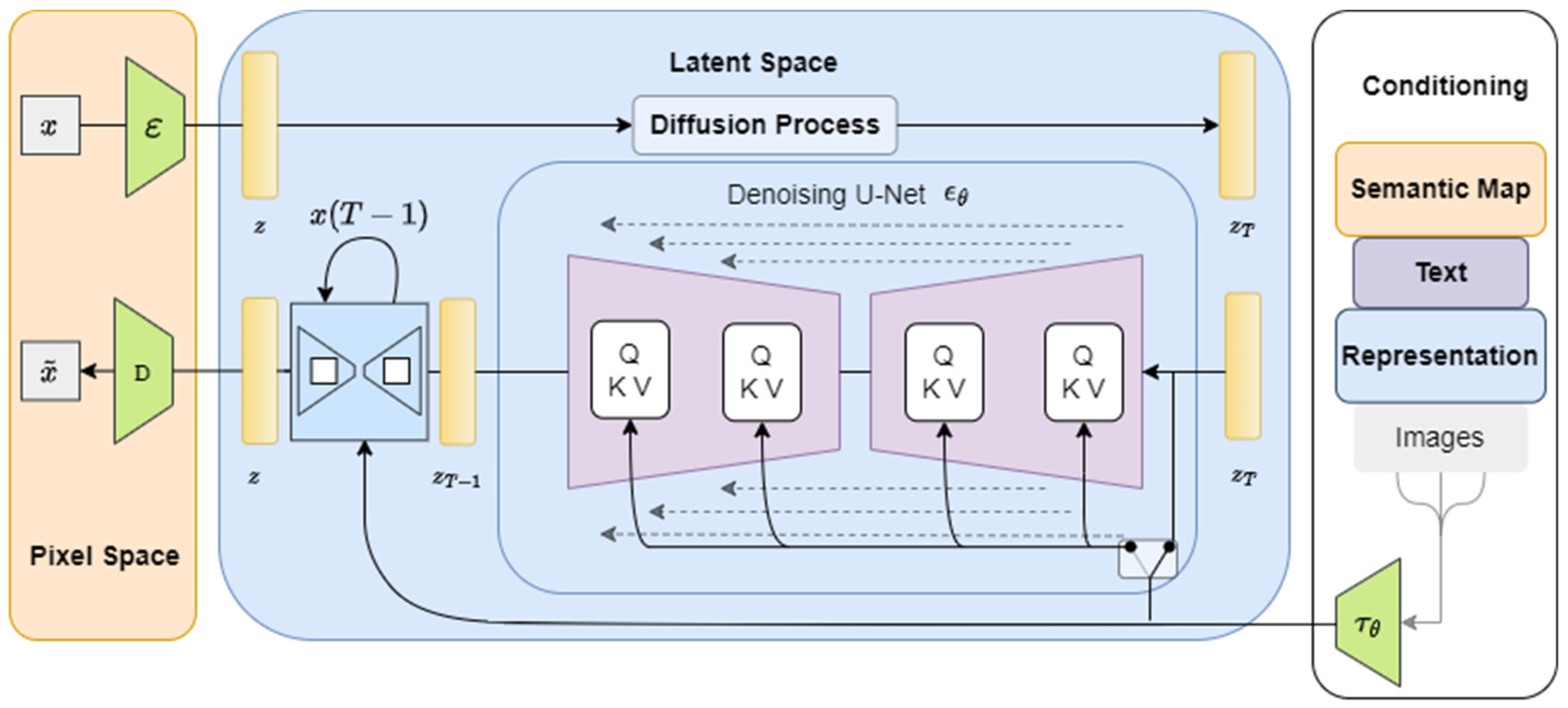
Latent Diffusion Models (LDMs) [29] are designed to improve the efficiency and scalability of diffusion models by operating in the latent space rather than the pixel space. By leveraging a pre-trained encoder–decoder architecture, LDMs reduce the dimensionality of the input data, allowing the diffusion process to focus on a more compact and semantically meaningful representation (Figure 7). This approach reduces computational costs while preserving the quality of the generated outputs. LDMs have been successfully used for high-resolution image generation, video synthesis, and other tasks requiring large-scale data modeling.
One of the most notable implementations of LDMs are Stable Diffusion [29]. Stable Diffusion builds upon the principles of DDPMs but introduces significant optimizations that make the approach scalable and efficient for high-resolution image generation. Unlike traditional diffusion models, Stable Diffusion operates in the latent space of pre-trained encoder–decoder models, such as Variational Autoencoders (VAEs). By working in a compressed representation space, Stable Diffusion significantly reduces the computational burden while maintaining fidelity and quality in the outputs, as depicted in Figure 8. This scalability has enabled its application in commercial and creative domains, where large-scale image synthesis and customization are required.

3.2.3. Text-Guided Diffusion

Text-Guided Diffusion Models such as DiffusionCLIP [32] or GLIDE [31] or ZeCon [33], extend diffusion models by incorporating textual information as a conditioning mechanism. These models utilize text embeddings derived from natural language descriptions to guide the denoising process, enabling the generation of images that align with the specified textual prompts. The integration of text guidance expands the applicability of diffusion models to creative and interactive tasks, including generating photorealistic images, creating artworks, and performing detailed image edits based on user-provided instructions.

3.2.4. Score-Based Generative Models

Score-based generative modeling [34,35] via stochastic differential equations unifies diffusion probabilistic frameworks and score-matching approaches. A forward SDE gradually perturbs data with noise, while the corresponding reverse-time SDE removes noise to recover the original distribution. The reverse dynamics depend solely on the time-dependent score of the perturbed data, i.e., the gradient of its log-density which is learned via neural networks using denoising score matching. Sampling then proceeds by integrating the learned score field backward in time with numerical SDE solvers or equivalent neural ordinary differential equation (ODE) techniques. Enhancements such as predictor–corrector schemes further reduce discretization error, and the same framework readily extends to inverse tasks like inpainting, class-conditional generation, and colorization.

3.2.5. Sampling Acceleration Techniques

Denoising Diffusion Implicit Models (DDIMs) [36] introduce a family of non-Markovian reverse processes that share the original DDPM training objective but permit a deterministic, implicit mapping from noise to data. By inverting the forward noising in closed form, DDIMs dramatically reduce the number of sampling steps trading off stochasticity for speed while preserving high sample quality and enabling semantically meaningful interpolation in the latent space.
DPM-Solver [37] treats diffusion sampling as solving an associated ordinary differential equation exactly. It analytically integrates the linear component of the diffusion ODE and then applies a dedicated high-order numerical solver with convergence guarantees. This yields high-fidelity samples in as few as 10–20 function evaluations without any additional training and achieves substantial speedups over prior sampling methods.

3.2.6. Large Language Diffusion Models

Large language diffusion models (LLDMs) [38] extend the denoising diffusion paradigm from continuous domains to discrete text data, treating language modeling as a principled forward–reverse masking process. A prime example is LLaDA (“Large Language Diffusion with mAsking”), which replaces the autoregressive next-token formulation with a masked diffusion framework: during pre-training, tokens are randomly masked at varying ratios t ∈ [0, 1], and a Transformer-based mask predictor is trained to recover all masked tokens simultaneously, optimizing an upper bound on the negative log-likelihood. At inference, LLaDA samples from a fully masked sequence by iteratively denoising and remasking, yielding bidirectional context modeling, parallelizable generation, and a natural trade-off between quality and speed. Empirically, LLaDA scales effectively to 8 B parameters—demonstrating in-context learning, instruction following, and reversal reasoning on par with leading autoregressive LLMs—while inherently avoiding the “reversal curse” and offering unique advantages such as non-causal attention and balanced forward/reverse performance.

3.2.7. Transformer-Based Models

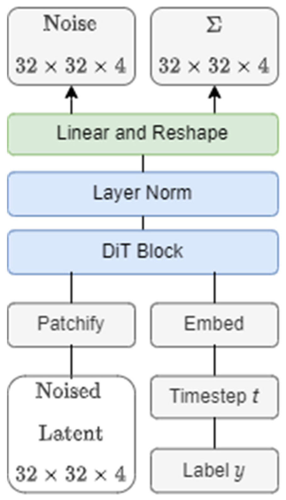
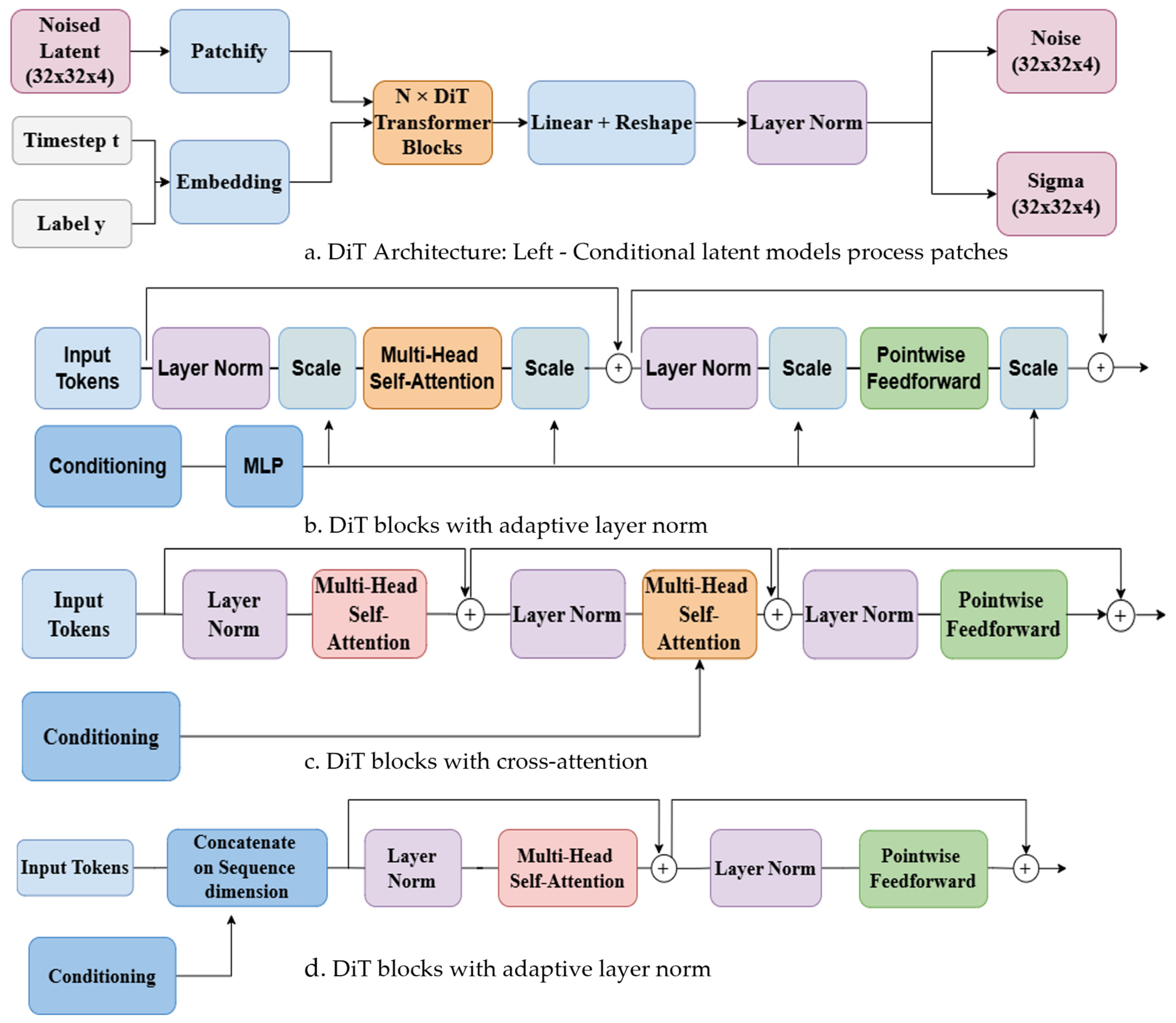
Transformers, particularly in autoregressive settings, have gained significant popularity for generative tasks across text, image, and video domains [39,40,41,42]. Their ability to model dependencies over large contexts makes them highly effective for high-level generative tasks such as story creation, video synthesis, and multimodal applications. These models leverage the self-attention mechanism to capture global relationships in data, making them well-suited for complex generation tasks. Transformer-based diffusion models, like Diffusion Transformers (DiTs) [43], represent a significant advancement by combining the strengths of Transformers with the noise-to-data mapping capability of denoising diffusion models. This integration enables DiTs to capture intricate dependencies in data while producing high-quality, detailed outputs, often surpassing traditional convolutional architectures in tasks like image and video generation. Within the family of Transformer-based diffusion models (as shown in Figure 9), there are several architectural variations that optimize their performance for specific applications:
Standard DiT Block
The foundational component of Diffusion Transformers uses adaptive layer normalization (adaLN) to dynamically adjust the feature scaling and shifting based on conditioning inputs. Combined with multi-head self-attention and feed-forward layers, this structure excels at modeling dependencies in noisy latent representations for high-quality data generation.
DiT Block with Cross-Attention
This variation incorporates a multi-head cross-attention mechanism, enabling the model to condition its output on external information such as text or labels. This is particularly powerful for text-to-image or text-to-video tasks, where the model needs to integrate semantic guidance into the generation process
DiT Block with In-Context Conditioning
This configuration concatenates conditioning information (e.g., labels or temporal data) directly to the input sequence, allowing the Transformer to jointly process input tokens and context in a unified manner. This setup is effective for scenarios requiring close interaction between data and context, such as temporal video generation or multimodal synthesis.
While Transformer-based diffusion models such as DiT [44] achieve excellent generation quality, their computational cost presents a significant obstacle for practical deployment. The standard self attention mechanism operates with quadratic complexity O(n^2) in the sequence length, meaning that as image resolution increases and the number of patch tokens grows, both memory consumption and computation time scale rapidly. For high resolution generation tasks, this bottleneck can render full attention infeasible without specialized hardware or distributed training setups. To mitigate this limitation, several lines of recent research have proposed efficient attention variants. Reformer [45] introduces locality sensitive hashing to approximate attention with reduced complexity. FlashAttention [46] provides an IO aware implementation that significantly reduces memory overhead while computing exact attention. Sparse attention mechanisms restrict the attention pattern to local or structured subsets of tokens, achieving substantial speedups with minimal quality degradation. These developments are critical for making Transformer-based diffusion models scalable to high resolution and real time applications, and represent an active area of ongoing research.

3.2.8. Consistency and Distillation-Based Models

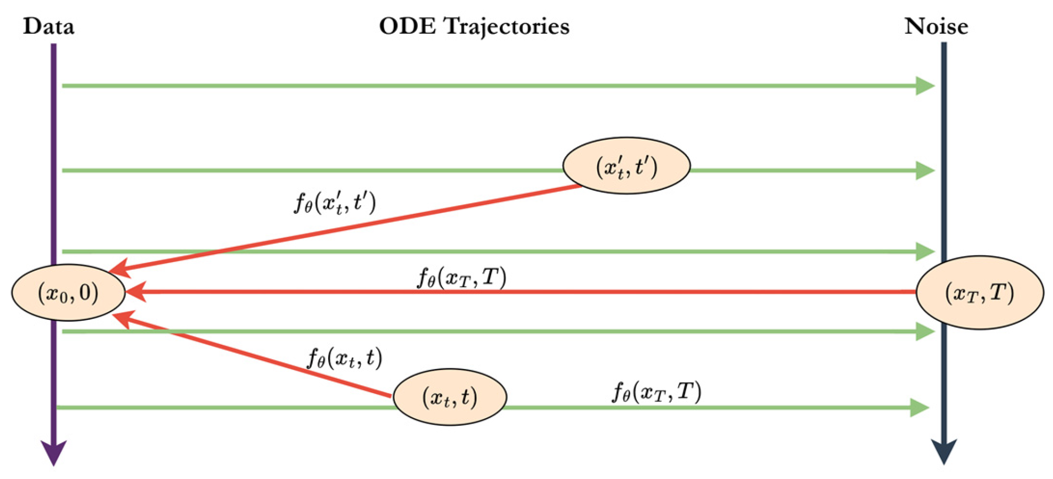
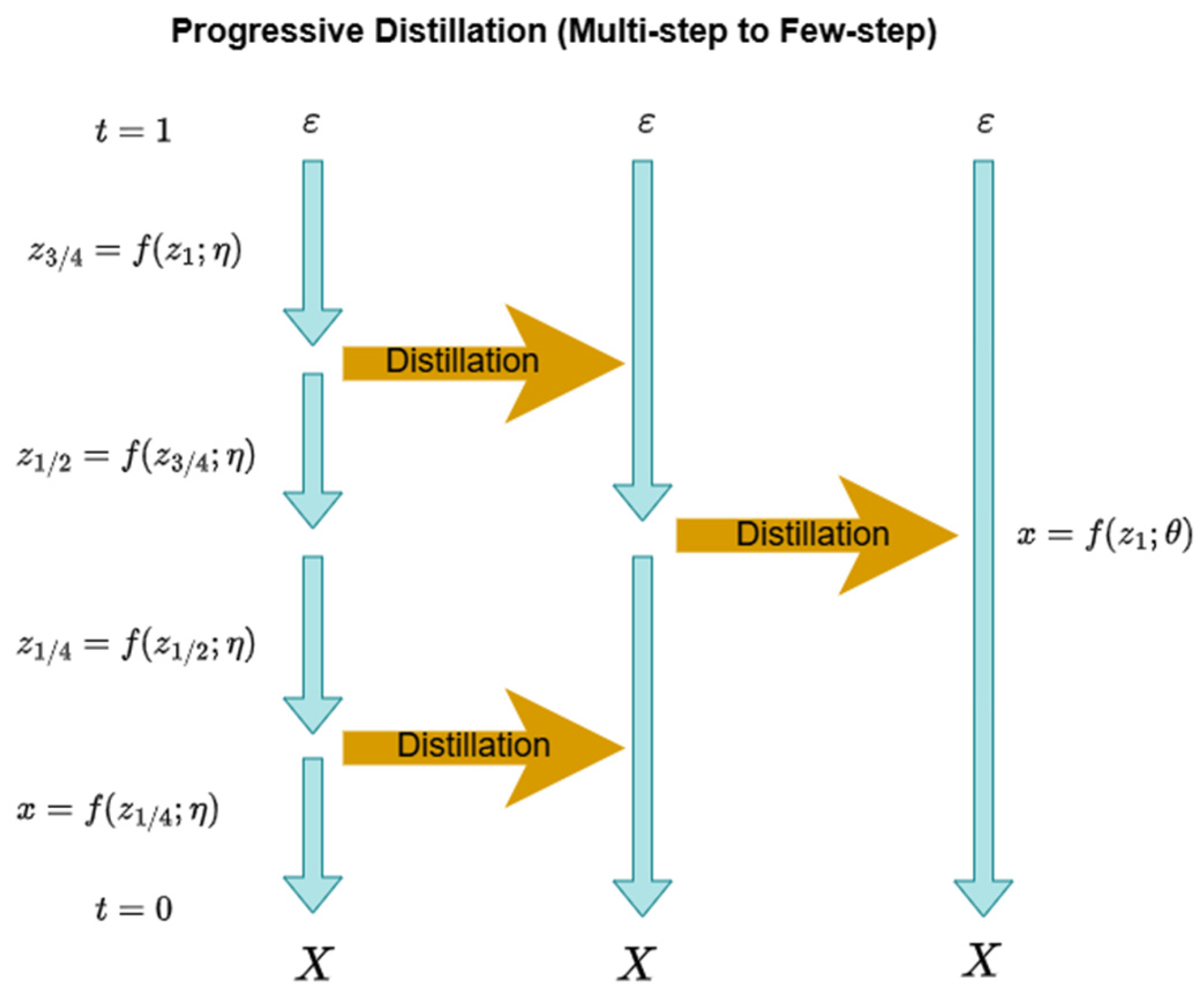
Consistency models [44,47,48] and distillation-based approaches [49] aim to reduce the number of sampling steps required for generation as depicted in Figure 10 and Figure 11. These methods train a model to produce consistent outputs across different noise levels, enabling few-step or even single-step generation. Such approaches significantly improve inference efficiency while maintaining sample quality, making them suitable for real-time applications.

3.2.9. Flow Matching and Rectified Flow Models

Flow matching [50] and rectified flow [51] approaches reformulate diffusion models as deterministic transformations between noise and data. Instead of modeling stochastic transitions, these methods learn a velocity field that maps samples from a simple distribution to the data distribution. This perspective simplifies training and enables efficient sampling using ordinary differential equation solvers.

3.2.10. Hybrid Diffusion Models

Hybrid approaches [27] combine diffusion models with other generative frameworks, such as variational autoencoders or adversarial models. These methods leverage the strengths of different paradigms, for example using diffusion for high-quality generation and adversarial training for sharper outputs. Such combinations enable improved performance in specific applications.
Summary of Diffusion Model Variant Tradeoffs: The diffusion model variants described above offer complementary strengths and limitations. DDPM provides a principled probabilistic framework with stable training, but its reliance on pixel space computation and hundreds to thousands of sampling steps limits scalability. Latent Diffusion Models address the computational bottleneck by operating in a compressed representation space, enabling high resolution generation at reduced cost, though they introduce a dependency on the quality of the pretrained encoder and decoder. Score-based SDE models offer theoretical elegance and continuous time formulations that unify discrete and continuous diffusion, but their practical implementation can be sensitive to the choice of SDE solver and discretization scheme. Transformer-based approaches such as DiT achieve excellent quality by leveraging global self attention, but face quadratic complexity challenges at high resolutions. Consistency models and distillation-based methods dramatically improve inference speed, though often with some reduction in sample diversity or quality. Flow matching approaches offer deterministic, efficient sampling but are relatively newer and less extensively benchmarked. These tradeoffs reinforce the value of the multi dimensional taxonomy introduced in Section 3.3, which allows systematic comparison of models along independent design axes rather than treating each variant as a monolithic architecture.

3.3. Taxonomy of Diffusion Models

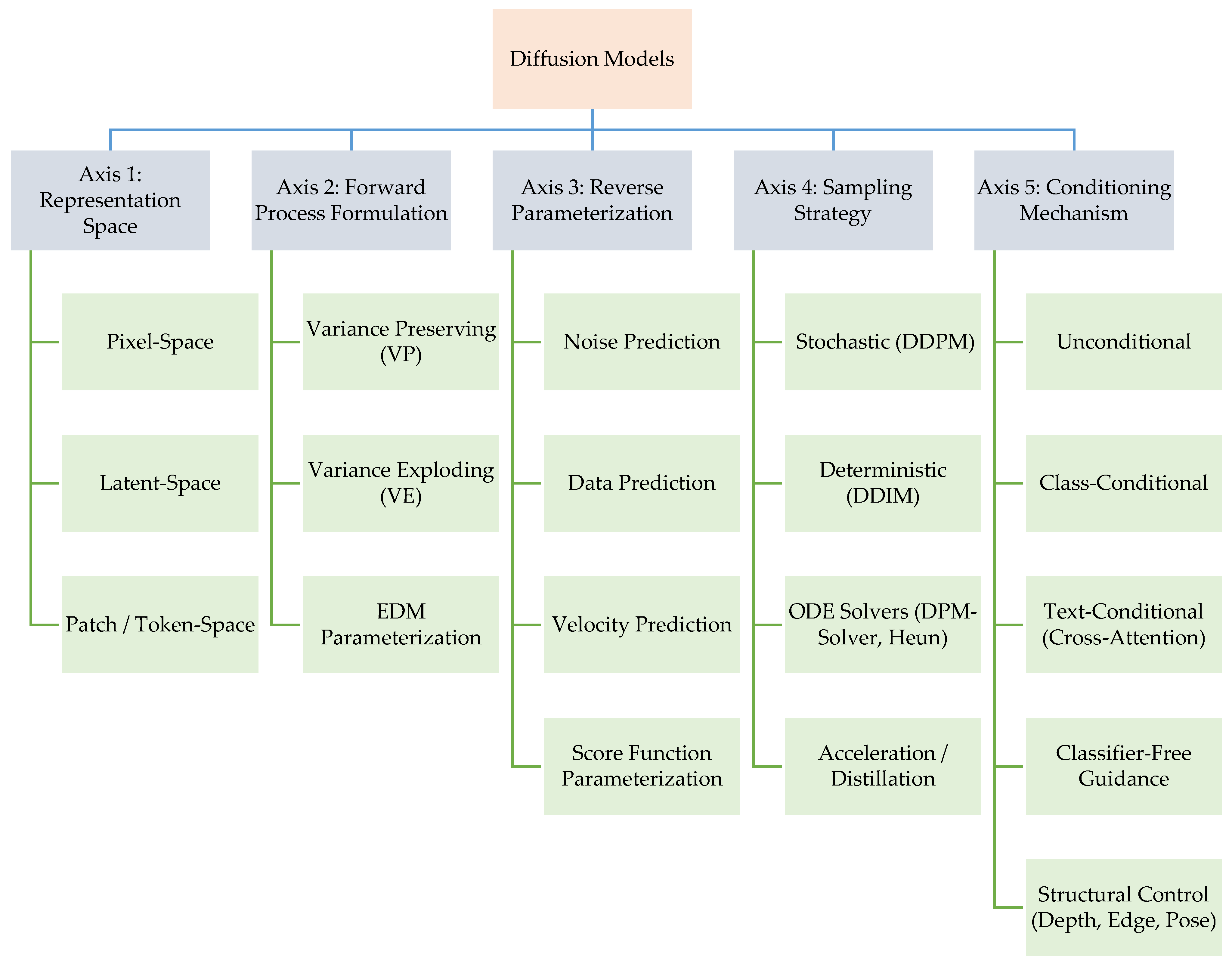
Diffusion models can be described along multiple design dimensions rather than a single architectural category. To systematically organize existing methods and to address the gap identified in prior surveys that typically classify models along a single dimension, we categorize diffusion models along five orthogonal axes (as illustrated in Figure 12):
  • Representation Space;
  • Forward Process Formulation;
  • Reverse Parameterization;
  • Sampling Strategy;
  • Conditioning Mechanism.
Each axis captures a distinct design choice that influences model behavior, computational cost, and applicability across domains. This taxonomy provides a structured view of diffusion models and enables comparison across different formulations and architectures.

3.3.1. Axis 1: Representation Space

This axis describes the space in which the diffusion process operates. Diffusion models can be applied directly to high-dimensional data (e.g., pixels) or to a transformed representation that reduces dimensionality or introduces structure. The choice of representation affects computational cost, memory requirements, and the type of patterns the model can capture.
  • Pixel-Space: Diffusion is applied directly to raw data (e.g., images). This provides full fidelity but is computationally expensive.
  • Latent-Space: Data are first encoded into a lower-dimensional representation, and diffusion is performed in this latent space. This reduces computational cost while preserving semantic structure.
  • Patch/Token-Space: Data are represented as discrete or continuous tokens (e.g., patches or embeddings), enabling transformer-based diffusion models.

3.3.2. Axis 2: Forward Process Formulation

This axis defines how noise is added to the data during the forward diffusion process. The forward process gradually perturbs data into noise through a sequence of stochastic transformations. Different formulations correspond to different noise schedules and continuous-time interpretations.
  • Variance Preserving (VP): Maintains a bounded variance during the diffusion process, commonly used in discrete-time diffusion models such as DDPM.
  • Variance Exploding (VE): Increases variance over time, often used in score-based generative models formulated via stochastic differential equations.
  • EDM Parameterization: A continuous formulation that generalizes noise scaling and improves stability and sampling efficiency.

3.3.3. Axis 3: Reverse Parameterization

This axis describes what the model predicts during the reverse diffusion process. The reverse process is implemented using a neural network that predicts a quantity related to the clean data. Different parameterizations correspond to different training objectives and numerical stability properties.
  • Noise Prediction (ε-prediction): The model predicts the noise added at each step. This is the standard formulation in DDPM.
  • Data Prediction (x0-prediction): The model directly predicts the original clean data.
  • Velocity Prediction (v-prediction): The model predicts a combination of data and noise, improving stability in some settings.
  • Score Function Parameterization: The model predicts the gradient of the log-density (score), connecting diffusion models to score-based generative modeling.

3.3.4. Axis 4: Sampling Strategy

This axis defines how samples are generated from the learned reverse process. Sampling involves iteratively applying the reverse dynamics. Different strategies trade off between sample quality, computational cost, and stochasticity.
  • Stochastic Sampling (DDPM): Uses a Markov chain with injected noise at each step, leading to diverse samples but higher computational cost.
  • Deterministic Sampling (DDIM): Uses a non-Markovian deterministic mapping, enabling faster generation with fewer steps.
  • ODE-Based Solvers (e.g., DPM-Solver, Heun): Treat sampling as solving an ordinary differential equation, allowing efficient high-quality generation.
  • Acceleration/Distillation: Reduces the number of sampling steps through learned or approximated processes.

3.3.5. Axis 5: Conditioning Mechanism

This axis describes how additional information is incorporated into the generation process. Conditioning allows diffusion models to generate outputs aligned with external inputs such as labels, text, or structural constraints.
  • Unconditional: Generation is based only on the learned data distribution.
  • Class-Conditional: Conditioning on discrete labels.
  • Text-Conditional (Cross-Attention): Uses text embeddings to guide generation.
  • Classifier-Free Guidance (CFG) [52]: Combines conditional and unconditional predictions to control generation strength without requiring a separate classifier.
  • Structural Control (e.g., depth, edges, pose): Incorporates spatial constraints or control signals.
Diffusion models are not defined by a single architectural category. Instead, a given model corresponds to a combination of design choices across these axes. Each axis represents an independent dimension of the model design space, and different diffusion models can be understood as selecting specific configurations along these dimensions. This perspective enables a systematic comparison of models that may differ in one or more aspects while sharing common components.

3.4. Mapping Diffusion Models to Taxonomy

To demonstrate the practical relevance of the proposed taxonomy, we map representative diffusion models to the defined axes. Each model corresponds to a specific configuration across the five dimensions, illustrating how different design choices lead to distinct modeling behaviors as illustrated in Table 3.
Table 4 illustrates how representative diffusion models map onto the proposed five dimensional taxonomy. Each row corresponds to a specific model configuration, and each column represents one of the five design axes. This mapping reveals that many widely used models share common choices along certain axes (for example, most employ Variance Preserving forward processes and noise prediction) while differing on others (such as representation space or conditioning mechanism). This structured view enables researchers to identify underexplored combinations of design choices and to reason systematically about how changing one dimension (e.g., switching from pixel space to latent space) affects other aspects of model behavior. We note that quantitative performance benchmarks (such as FID scores) are intentionally omitted from this table, as they depend heavily on dataset, resolution, and implementation details; Section 8 provides a dedicated empirical comparison along these lines.

4. Noise in Imaging and Video Domains

This section explores noise in imaging and video domains, categorizing it by domain, source, and distribution. Noise varies significantly across applications such as low-light photography, medical imaging, and remote sensing, creating unique challenges for clarity and accuracy. The sources of noise include sensor limitations, environmental effects, and compression artifacts, and it can be classified as signal-independent or signal-dependent. Noise also adheres to specific distributions (e.g., Gaussian or Poisson), which characterize its statistical behavior. Understanding these factors is critical for improving model robustness and achieving higher visual fidelity in generative and denoising tasks.

4.1. Domain

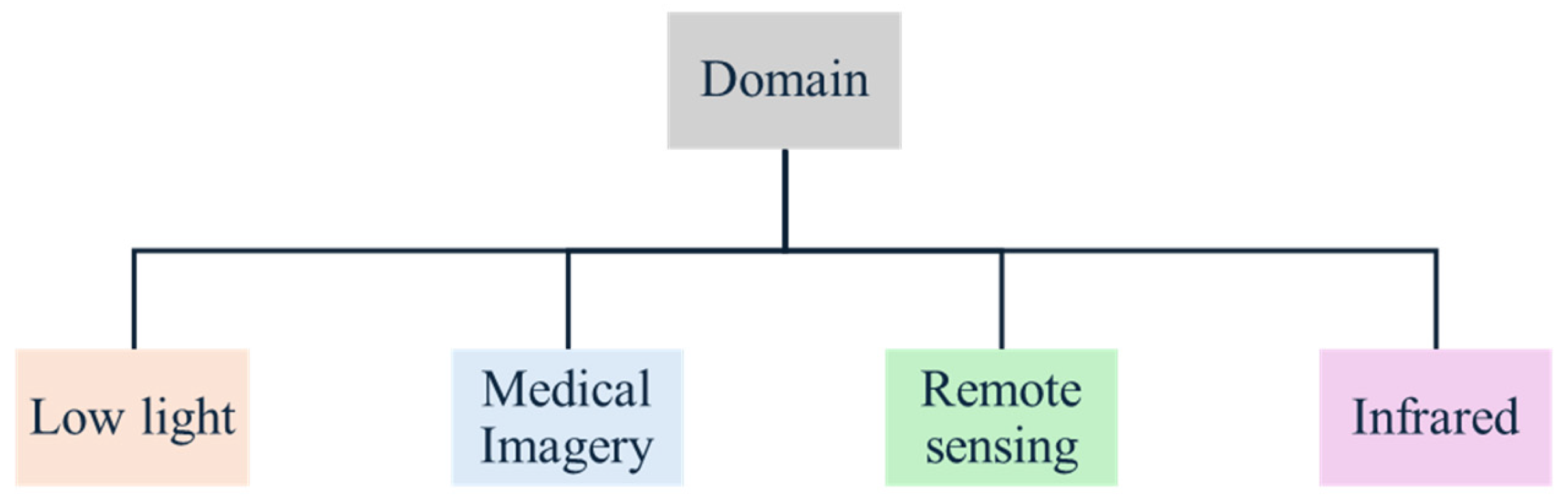
Imaging systems across domains (Figure 13) introduce unique types of noise that degrade visual fidelity and complicate image interpretation. From photon shot noise in low-light photography to speckle in ultrasound and atmospheric distortion in remote sensing, understanding the statistical properties of noise is essential for effective denoising. This section outlines major domain-specific noise types and their implications for generative modeling.

4.1.1. Low Light Images

Images captured in low-light conditions often suffer from shot noise or quantum noise, which arises as grainy artifacts or random color speckles due to the sensor’s increased sensitivity in dim lighting. This type of noise results from the inherent randomness of photon arrivals at the sensor and is modeled by a Poisson distribution, where the variance of the noise is directly proportional to the signal intensity. Due to photon limitations in dim lighting, this noise significantly degrades image quality by reducing detail and color fidelity. Let I(x) represent the pixel intensity, and n(x) ∼ Poisson (I(x)). The observed noisy pixel intensity is given by:
I x = I x + n ( x )
where n(x) introduces noise, and denoising aims to minimize the effect of n(x). Promising advancements, such as the application of deep image priors, leverage deep learning architectures to effectively learn and mitigate noise patterns, enabling improved low-light denoising directly from image data [53,54].

4.1.2. Medical Imaging

In medical imaging, noise can hinder accurate diagnosis and analysis. Ultrasound, for example, is impacted by speckle noise, a granular noise arising from the coherent nature of the imaging process. Speckle noise obscures fine details in anatomical structures, making it difficult for medical professionals to interpret images.
This noise can be modeled using a Rayleigh distribution, where the probability density function is given by:
p x = x s   2 e x p x   2 2 s   2 ,   x 0
where σ represents the scale parameter of the distribution.
Variational methods, along with compressed sensing techniques, have been explored to enhance image clarity and preserve detail in medical imaging, improving the diagnostic potential of such images while reducing the speckle noise [55,56].

4.1.3. Remote Sensing

Remote sensing applications, such as multispectral and synthetic aperture radar (SAR) imaging, are often affected by atmospheric effects, sensor noise, and quantization errors. InSAR (Interferometric SAR) in particular faces noise challenges such as temporal and spatial decorrelation, as well as atmospheric disturbances, complicating the interpretation of geospatial and environmental changes. Gaussian noise is frequently assumed for its simplicity and applicability in many scenarios:
p x = 1 2 π s   2 e x p ( x m )   2 2 s   2
where m is the mean, and s is the standard deviation of the noise.
Denoising methods, including variational and bilateral filtering techniques, have shown effectiveness in enhancing image quality by mitigating these issues [57,58].

4.1.4. Infrared Imaging

Infrared images, widely used in surveillance and environmental monitoring, often suffer from electronic noise and thermal variations due to detector non-uniformity. This noise can obscure crucial details, reducing the precision of thermal measurements. Techniques like multiscale wavelet denoising and total variation-based enhancement are employed to improve the signal-to-noise ratio, providing clearer insights in applications ranging from night vision to environmental studies [59,60,61]. If I is the image and W(⋅) represents the wavelet transform, the denoised image I’ can be obtained as:
I = W 1 ( T ( W I ) )
where T(⋅) is a thresholding function applied to suppress noise in the wavelet domain.

4.2. Sources of Noise

Noise in images and videos arises from various sources, each contributing distinct distortions that impact the clarity and fidelity of the data. These noise sources are deeply intertwined with the imaging process, influenced by sensor limitations, environmental conditions, and data encoding methods. Noise can be broadly classified into signal-independent and signal-dependent categories. Signal-independent noise remains constant across varying image content, while signal-dependent noise changes in intensity or distribution based on the captured scene or signal. Understanding these noise sources is critical for designing robust generative models, particularly in denoising diffusion models, which aim to reconstruct clean data from noisy observations. The subsequent discussion outlines the major sources of noise, detailing their origins, statistical properties, and implications for image and video generation tasks.

4.2.1. Sensor Noise

Sensor noise, a fundamental source of distortion, arises during the image capture process. This includes photon shot noise, which results from the inherent randomness in photon arrivals at the sensor. Photon shot noise becomes particularly pronounced in low-light conditions, where fewer photons are available, leading to grainy or speckled patterns. Mathematically, this noise can be modeled as
I x = I x + n s e n s o r x ,     n s e n s o r x ~ G a u s s i a n ( 0 ,   s   2 )
where n s e n s o r (x) is Gaussian-distributed noise with zero mean and variance s 2 .
In addition to photon noise, thermal noise is caused by the thermal agitation of electrons within the sensor that further degrades image quality. Advanced sensor technologies and post-processing algorithms aim to mitigate these effects, but they remain a significant challenge, particularly in high-speed imaging or low-light scenarios.

4.2.2. Compression Artifacts

Compression artifacts are distortions introduced during lossy compression techniques such as JPEG. These artifacts manifest as blocky patterns or “ringing” effects, particularly around high-frequency image components like edges or textures. The root cause lies in the quantization and truncation of image data during compression, which simplifies storage but sacrifices fidelity. Such artifacts can be mathematically modeled as:
I x = I x + n c o m p r e s s i o n x
where n c o m p r e s s i o n x represents the distortions introduced during compression.
Compression noise is especially detrimental in tasks requiring high-frequency detail preservation, such as medical imaging or artistic rendering. Advanced denoising approaches, such as total variation minimization or transform-domain techniques, are commonly employed to suppress these artifacts and restore visual quality.

4.2.3. Quantization Noise

Quantization noise emerges during the digitization process, where continuous analog signals are converted into discrete digital values. This process introduces a granularity in the image, particularly noticeable in low-intensity or flat regions. A specific manifestation of quantization noise is speckle noise, prevalent in coherent imaging systems such as ultrasound and synthetic aperture radar (SAR). Speckle noise arises from the coherent summation of scattered wavefronts, leading to granular distortions that obscure fine details.
I x = I x + n q u a n t i z a t i o n
where n q u a n t i z a t i o n represents the error introduced by finite-level quantization.
Quantization noise is particularly challenging in applications requiring high precision, such as depth estimation or 3D reconstruction. Advanced denoising techniques, such as speckle reduction filtering or adaptive quantization, have been developed to address this issue.

4.2.4. Low Light/High ISO Noise

Low-light conditions exacerbate noise due to the reduced availability of photons, leading to shot noise. Additionally, the amplification of sensor signals under high ISO settings introduces read noise, further degrading the image. The combined effect results in visible distortions, such as grainy textures or color inconsistencies, which obscure image details. Mathematically, this noise can be described as:
I x = I x + n s h o t x +   n r e a d x
State-of-the-art denoising algorithms, such as BM3D (Block-Matching 3D), are highly effective in these scenarios, leveraging non-local filtering and collaborative patch processing to reduce noise while preserving image details.

4.2.5. Environmental Effects (Atmospheric Distortion)

Environmental factors, such as atmospheric distortion, introduce additional noise in imaging and video data. These effects, often referred to as ground truth noise, are common in remote sensing applications where images are captured over long distances or through turbulent media. Distortions include scattering, absorption, and refraction, which alter the intensity and spatial coherence of the captured signal. This noise can be modeled using Gaussian distributions for simplicity:
p x = 1 2 π s   2 e x p ( x m )   2 2 s   2
However, atmospheric noise often exhibits non-Gaussian characteristics in real-world scenarios, requiring specialized denoising strategies such as variational filtering or wavefront correction to mitigate its effects.

4.2.6. Implications for Diffusion Models

The noise characteristics observed across imaging domains introduce important challenges for diffusion-based generative models. While classical denoising approaches often rely on explicit noise models such as Gaussian, Poisson, or Rayleigh distributions, standard diffusion models typically assume a Gaussian forward noise process. Consequently, the learned reverse process is optimized for Gaussian perturbations, which may not accurately reflect real-world noise conditions.
In practical settings, imaging data frequently exhibits non-Gaussian noise, including photon shot noise in low-light photography, speckle noise in medical imaging, and atmospheric distortions in remote sensing. These discrepancies between assumed and actual noise distributions can degrade denoising performance and limit generalization.
To address this mismatch, recent research explores several strategies, including adapting the forward noise process, incorporating domain-specific conditioning, and fine-tuning models on target distributions. Understanding the statistical properties of noise in different domains is therefore critical for improving the robustness and fidelity of diffusion-based generative models.

4.3. Noise Distributions

Noise distributions are closely linked with various types of noise and sensor technologies. Among these, the Gaussian noise family, which includes Laplacian and Generalized Gaussian noise, represents a common model for many types of real-world noise. On the simpler end of the spectrum, Uniform and Impulse noise distributions provide basic models for random fluctuations. More complex distributions such as Rayleigh, Poisson, Gamma, and Exponential are associated with specific phenomena across different modalities. Each of these distributions characterizes the statistical behavior of noise in different imaging contexts, reflecting the diverse nature of disturbances that can affect signal quality.

4.4. Practical Guidance for Noise Aware Diffusion Model Design

The preceding sections establish that different imaging domains exhibit distinct noise characteristics, each governed by a specific statistical distribution. For practitioners designing diffusion models for domain-specific applications, understanding how to align the forward process formulation and data preprocessing strategy with the target noise type is critical for achieving robust performance. Table 5 summarizes recommended design considerations for several common noise scenarios encountered in practice.
This table is intended as a starting point for model developers. The optimal configuration will depend on the specific dataset characteristics, resolution requirements, and computational constraints of each application. In cases where multiple noise types coexist (e.g., combined shot noise and read noise in low light high ISO settings), a combination of preprocessing steps and an appropriately flexible forward process formulation may be necessary.

5. Denoising Strategies in Diffusion Models

Diffusion models rely on a learned denoising process to progressively reconstruct data from noise. During training, a clean image x is gradually perturbed by Gaussian noise n, producing a noisy version x + n. The model then learns a denoising function Dθ that approximates the reverse of this process:
x =   D θ   x + n
captures the core idea, that diffusion denoising is in fact an iterative process, where the model removes noise step-by-step using learned conditional distribution. The goal of this process is not to recover the original image exactly, but to generate a new sample drawn from the same data distribution. In supervised denoising or image reconstruction, quality is often assessed using metrics like Peak Signal-to-Noise Ratio (PSNR) and Structural Similarity Index (SSIM). However, for unconditional generation, especially in diffusion models, distribution-based and perceptual metrics such as Fréchet Inception Distance (FID), CLIPScore, and LPIPS are more appropriate.
While diffusion models perform denoising as a core generative mechanism, traditional denoising techniques—like median filters, BM3D, or wavelet shrinkage—can still be applied as pre-processing (to clean training data) or post-processing (to refine outputs from fast samplers). These approaches fall into two categories:
(1) In-model denoising, which refers to the learned, iterative reverse process that defines diffusion-based generation; and (2) External denoising techniques, which include classical and learned filters applied before or after generation to clean training data or refine outputs.
The following subsections elaborate on these two categories, highlighting their principles, roles, and practical distinctions.

5.1. In-Model Denoising Techniques in Diffusion Models

In diffusion models, “denoising” refers to the process by which a neural network approximates the reverse of a fixed forward noise process applied during training. This learned process lies at the heart of generation. The network is trained to predict one of three possible targets:
  • ε: the noise added at each step.
  • x0: the original uncorrupted data.
  • v: a combination of x0 and ε (velocity formulation), which stabilizes training and improves conditioning.
The forward process progressively adds Gaussian noise using a schedule (e.g., linear, cosine), which determines how aggressively noise is injected over time. The reverse process is implemented using various samplers:
  • DDPM (stochastic sampling);
  • DDIM (deterministic, non-Markovian);
  • DPM-Solver, EDM (few-step ODE-based solvers).
Classifier-free guidance (CFG) [52] modifies the denoised output at each step to steer it toward conditional inputs (e.g., text), trading off between fidelity and diversity.

5.2. External Denoising Techniques

External denoising techniques are not part of the diffusion model architecture. They can be used to:
  • Pre-process training data (e.g., removing compression artifacts);
  • Post-process outputs (e.g., cleaning up residual noise from low-step samplers).
These include both classical and learned methods, each with specific properties. To guide practitioners in selecting appropriate external denoising techniques within a diffusion model pipeline, the following application level recommendations are offered. For preprocessing of training data, bilateral filtering is particularly suited for smoothing non Gaussian noise (such as speckle noise in medical ultrasound datasets) because its edge-preserving properties retain structural detail that the diffusion model needs to learn. Median filtering is effective for removing impulse noise (salt and pepper artifacts) from corrupted training images. For post processing of generated outputs, BM3D [62] is recommended for fine detail preservation and enhancement, especially when outputs from accelerated samplers (e.g., few step DDIM or DPM Solver) exhibit residual high frequency noise. Wavelet transform denoising is well suited for domain-specific post processing in medical imaging and remote sensing, where multi scale analysis allows targeted noise suppression without over smoothing diagnostically relevant features. Transform domain methods (DCT, Fourier) are appropriate for removing structured artifacts such as banding or ringing introduced by compression or quantization.

5.2.1. Mean Filter

Given an input image I, with its pixels at position (u,v) denoted by I (u,v), the mean filter operates by calculating the average value within a local neighborhood R surrounding each pixel position (u,v). For each output pixel I′(u,v), the mean value is computed as follows:
I ( u , v ) = 1 R ( i , j ) R I ( u + i , v + j )
In this formula, i and j represent offsets within the local neighborhood R from the central pixel position (u,v). This process replaces each pixel in the original image with the mean (average) value of its neighboring pixels, effectively smoothing the image and reducing noise.

5.2.2. Median Filter

Given an input image I, with its pixels at position (u,v) denoted by I(u,v), the median filter operates by calculating the median value within a local neighborhood W surrounding each pixel position (u,v). For each output pixel I′(u,v), the mean value is computed as follows:
I ( u , v ) = m e d i a n   { I ( u + i , v + j )   |   ( i , j )     W   }
where I′(u,v) is the output pixel value after applying the median filter, and W represents the window of neighbors around the pixel (u,v) including itself. The sizes of W can vary but are typically chosen to be odd, such as 3 × 3, 5 × 5, etc., to ensure there is a central pixel. Unlike the mean filter, which uses the average of the pixel values, the median filter uses the median value, which is less sensitive to outliers. This characteristic makes the median filter particularly effective at removing ‘salt and pepper’ noise from images, while preserving edges better than a mean filter.

5.2.3. Non-Local Filtering

Block-matching 3D (BM3D) is an advanced non-local filtering algorithm that operates across the entire image. The process begins with block matching (BM), where the algorithm searches the image to find blocks (small sub-regions of the image) that are similar to each other. These similar blocks are then grouped together to form 3D data arrays, or “cubes.” Once the blocks are arranged into 3D cubes, they are collectively filtered to reduce noise. This is done by exploiting the redundancy of structural information in the grouped blocks. After the filtering process, the denoised blocks are reassembled back into the image, ensuring that the overall structure and details are preserved while noise is significantly reduced. The parameter σ plays a crucial role in BM3D. It is an estimation of the noise level within the image, acting as a control measure for the denoising strength. By adjusting σ, users can fine-tune the extent of denoising applied, balancing noise reduction and detail preservation according to the specific needs of the image. This makes BM3D a highly effective and adaptable denoising technique for a wide range of applications.

5.2.4. Transform Domain Denoising

Transform domain denoising applies filters in the frequency or wavelet space, where noise and signal components are more separable. By selectively attenuating high-frequency components, noise can be reduced while preserving essential image details.
One common approach is Discrete Cosine Transform (DCT) denoising, where the image is transformed into the DCT domain. Noise, which primarily resides in higher frequencies, is suppressed by thresholding or smoothing high-frequency coefficients. The denoised image is then reconstructed via inverse DCT:
I x = D C T 1 ( T ( D C T I x ) )
This method effectively removes compression artifacts and fine-grained noise, enhancing image quality in generative tasks.
Similarly, Fourier Transform denoising filters high-frequency noise by applying low-pass filters in the Fourier domain, making it particularly useful for structured noise or periodic artifacts. The ability to operate in the transform domain allows for flexible, high-fidelity denoising in diffusion models.

5.2.5. Bilateral Filtering

Bilateral filtering is a non-linear, edge-preserving denoising technique that smooths images while retaining sharp edges. Unlike mean or median filters that uniformly apply smoothing, bilateral filters consider both spatial proximity and pixel intensity differences to reduce noise selectively. The denoised pixel value I’(u,v) is calculated as:
I u , v = 1 W i , j ϵ W I u + i , v + j f d | I u + i , v + j I u , v | f s | i , j u , v |
where fd represents the intensity difference weight, fs is the spatial weight, and W normalizes the sum. This approach effectively suppresses noise while preserving textures and important details, making it suitable for enhancing the visual fidelity of generated images in diffusion models.

5.2.6. Wavelet Transform Denoising

Wavelet transform denoising involves decomposing an image into multiple frequency bands using wavelet coefficients. Noise typically manifests at higher-frequency bands, while essential image details reside in lower-frequency bands. By thresholding or shrinking the wavelet coefficients corresponding to high-frequency components, the noise is reduced without blurring the image.
I x = W 1 ( T ( W I x ) )
where W and W−1 denote the wavelet transform and its inverse, respectively, and T is a thresholding function applied to the coefficients. This method effectively balances denoising with detail preservation, enhancing the quality of outputs generated by diffusion models across domains like medical imaging and remote sensing.

5.2.7. Denoising Autoencoders (DAE)

Denoising autoencoders are neural networks trained to reconstruct clean data from noisy inputs. During training, noise is artificially added to input data, and the autoencoder learns to predict the original uncorrupted image. This process enhances the model’s robustness and helps diffusion models generate high-quality images by mitigating noise artifacts during the denoising steps.
x = D θ x + n
where Dθ represents the autoencoder with learnable parameters θ. DAEs contribute significantly to the noise reduction stages of diffusion processes, particularly for high-dimensional data like images and videos. While the expression x′ provides intuition about denoising, diffusion models apply this operation iteratively across many timesteps. Each step removes a small portion of noise conditioned on the learned distribution, using samplers such as DDPM, DDIM, or ODE-based solvers.
These additional techniques complement the traditional methods described earlier, offering diverse approaches to denoising that improve the performance and visual quality of diffusion models in various generative tasks. To summarize and compare these methods, Table 6 presents a comparative analysis of widely used external denoising techniques in diffusion models, highlighting their key characteristics and performance. These techniques are not part of the in-model denoising in diffusion models. They may be used as preprocessing (e.g., to clean training data) or post-processing (e.g., to remove residual noise after fast sampling).

5.3. Architectural and Denoising Design Choices Across Applications

Table 7 presents use cases of diffusion models, associated architectures, and optional post-processing techniques. It is important to note that external filters such as BM3D or median filtering are not part of the core model architecture. They may be used after sampling to refine visual outputs, particularly in tasks requiring very high image fidelity.

6. Datasets

Datasets play a critical role in the development and evaluation of generative models, particularly diffusion models, which rely on large-scale and diverse data distributions to learn high-fidelity generation. The choice of dataset directly influences model performance, generalization, and the ability to generate realistic outputs across different domains.
Generative modeling tasks span a wide range of modalities, including images, videos, 3D scenes, and multimodal data. As a result, datasets vary significantly in scale, annotation type, and domain specificity. Large-scale datasets such as ImageNet and LAION-5B enable training of high-capacity models, while domain-specific datasets such as KITTI or medical imaging collections support specialized applications.
To provide a structured overview, datasets used in diffusion and generative modeling can be broadly categorized based on their primary application:
  • Image generation datasets, such as ImageNet, LSUN, and FFHQ, which are commonly used for unconditional and class-conditional generation;
  • Text-to-image datasets, including LAION-5B, CC3M, and CC12M, which enable multimodal conditioning;
  • Video datasets, such as Kinetics-700 and Vimeo90K, used for temporal generation and motion modeling;
  • 3D and scene datasets, including ShapeNet, SUNCG, and Matterport, supporting spatial and geometric modeling;
  • Autonomous driving datasets, such as KITTI and Cityscapes, which provide structured real-world environments;
  • Domain-specific datasets, including medical, remote sensing, and infrared imaging datasets, which introduce unique noise characteristics.
These datasets differ not only in scale but also in annotation richness, ranging from simple labels to dense segmentation maps, captions, and multimodal annotations. Such variations influence how diffusion models are trained, particularly in conditioning mechanisms and evaluation strategies. Table 8 provides a curated list of commonly used datasets in diffusion and generative modeling, along with their characteristics and typical applications.

Implications of Dataset for Diffusion Models

The choice of dataset directly affects the performance and design of diffusion models. Large-scale datasets with diverse distributions enable better generalization and higher-quality generation. Multimodal datasets, such as image–text pairs, are essential for conditional diffusion models, particularly in text-to-image generation. Domain-specific datasets introduce additional challenges, including non-Gaussian noise distributions and varying data characteristics. In such cases, diffusion models may require adaptation of the forward process or fine-tuning to account for domain-specific noise patterns. Consequently, dataset selection plays a central role in determining the effectiveness of diffusion models across different applications, from high-resolution image synthesis to video generation and scientific imaging.

7. Evaluation Metrics

Evaluating the quality of outputs from diffusion models depends heavily on the task: for reconstruction tasks (e.g., super-resolution, inpainting), pixel-level metrics like PSNR and SSIM may be used; however, for unconditional generation or text-to-image tasks, distribution-based and perceptual metrics are preferred. Below, we summarize commonly used evaluation metrics, their strengths and limitations, and appropriate use cases.

7.1. Peak Signal-to-Noise Ratio (PSNR)

The Peak Signal-to-Noise Ratio (PSNR) [122] measures pixel-wise fidelity between a reconstructed image and its ground truth. Mathematically, it is defined as:
P S N R = 10   ·   log 10 R 2 / M S E
where MSE (Mean Squared Error) represents the average squared difference between the original and reconstructed images, and R is the maximum pixel intensity (e.g., R = 255 for an 8-bit image). Higher PSNR values indicate lower distortion, but the metric correlates poorly with human perception. It is appropriate for supervised denoising or super-resolution tasks.

7.2. Structural Similarity Index (SSIM) and Multi-Scale SSIM (MS-SSIM)

Structural Similarity Index Metric (SSIM) [123] measures similarity by comparing corresponding patches in the ground truth and denoised images across three components: Luminance (l): The mean intensity of the patch; Contrast (c): The variation or standard deviation of the patch; and Structure (s): The correlation (or structural alignment) of the patch. Multi-Scale SSIM (MS-SSIM) [124] extends SSIM by assessing image quality at multiple scales (or resolutions), offering a more comprehensive, multi-scale perspective on perceptual fidelity. By comparing changes in luminance, contrast, and structure, SSIM and MS-SSIM yield a more perceptually aligned measure of image quality than purely pixel-based metrics. Higher SSIM or MS-SSIM scores indicate greater similarity to the ground truth, meaning the denoised image preserves essential visual characteristics in a way that aligns more closely with human perception. SSIM better reflects perceived quality than PSNR but still lacks semantic awareness.

7.3. Perceptual Similarity

Perceptual similarity metrics [125], such as those derived from deep neural networks (e.g., VGG or Learned Perceptual Image Patch Similarity), evaluate feature-level rather than pixel-level differences, aiming to more closely reflect human visual perception. These metrics comprise two main components: (1) Deep Feature Extraction, where images are passed through a pre-trained network (e.g., VGG) and intermediate layers capture edges, textures, and other discriminative features; and (2) Distance Calculation, often using L2 or cosine distance, between the feature maps of the denoised and ground-truth images. Lower distances in this feature space imply higher perceptual similarity. By focusing on semantic and structural attributes, perceptual similarity metrics align more accurately with how humans perceive visual differences. They are especially valuable in generative tasks where photo-realism or stylistic consistency is paramount, as opposed to pixel-perfect replication.

7.4. Mean Opinion Score (MOS)

Mean Opinion Score (MOS) [126] is a subjective evaluation measure rooted in human judgments. In an MOS test, a panel of participants rates the quality of denoised or reconstructed images on a predefined scale (e.g., 1 = bad, 5 = excellent). The average score across all participants and all evaluated images constitutes the final MOS. By capturing direct human perception, MOS provides indispensable insights into user experience, making it particularly valuable in domains such as entertainment, art, and consumer photography. However, conducting MOS evaluations can be time-consuming and expensive, and the results are inherently prone to biases, inconsistencies, and raters fatigue.

7.5. Fréchet Inception Distance (FID)

Fréchet Inception Distance (FID) [127] measures the distance between feature representations of real images and generated images. Features are typically extracted from a pre-trained Inception v3 network at a specific layer (often the pool3 or pool5 layer). If μ r , r represent the mean and covariance of real-image features, and μ g , g represent those of generated-image features, the FID is defined as:
F I D = μ r μ g 2 + t r r +   g 2 r g 1 2
Lower FID indicates that the distribution of generated images is closer to the distribution of real images in the learned feature space, suggesting higher quality and more realistic outputs. FID captures both mean shifts and covariance differences, making it sensitive to image quality and diversity. FID is widely used in evaluating GANs, diffusion models, and other generative frameworks for tasks like image synthesis and style transfer. Especially important for comparing how well a model captures the overall distribution of real data.

7.6. Fréchet Video Distance (FVD)

Fréchet Video Distance (FVD) [128] extends the idea of Fréchet Inception Distance (FID) framework to the video domain by comparing spatio-temporal features of real versus generated clips. Features are extracted from a pre-trained I3D network (typically at its final pooling layer), and clip-level activations are modeled as Gaussians for both real and generated sets. Computing the Fréchet (Wasserstein) distance between those Gaussians yields a single scalar that captures both spatial fidelity and temporal coherence, which correlates strongly with human judgments of video realism. Lower FVD implies that generated videos better match the real-video distribution in feature space. This metric has become standard for benchmarking video-generation models especially diffusion- and GAN-based approaches in tasks like text-to-video synthesis, future-frame prediction, and style transfer.

7.7. Inception Score (IS)

Inception Score (IS) [129] evaluates two properties of generated images. (1) Quality: How recognizable the generated images are to a classifier (often Inception v3); and (2) Diversity: How varied the generated images are across different classes. Mathematically, if p(y∣x) is the conditional label distribution of a generated image x under a pre-trained classifier, and p(y) is the marginal distribution of labels, the Inception Score is defined as:
I S = e x p E x D K L p y | x | |   p ( y )
where DKL is the Kullback–Leibler divergence. A High IS implies that each generated image is easily classifiable into a single class (good quality), and the distribution of classes across images is uniform or diverse. IS does not require real data for comparison and can be misleading if the label space is misaligned or if the classifier does not capture the nuances of generative quality. Often used in image generation tasks as a quick checkpoint of how “diverse and realistic” generated samples appear to a standard model.

7.8. Kernel Inception Distance (KID)

Kernel Inception Distance is a variation in Inception-based metrics that relies on Maximum Mean Discrepancy (MMD) in a feature space (again typically from Inception v3) [130]. Unlike FID, which assumes the feature distributions are multivariate Gaussian, KID uses a non-parametric kernel-based approach. The KID value is computed as:
M M D 2 = E x r , x r k ( x r , x r ) +   E x g , x g k ( x g , x g ) 2   E x r , x g k ( x r , x g )
where k is a polynomial kernel, and x r , x r   are real features, x g , x g are generated features. Lower KID indicates better alignment between the real and generated feature distributions. Non-parametric approach makes KID more robust when real data distributions deviate from Gaussian assumptions. KID can be a complement or alternative to FID, especially in scenarios where the Gaussian assumption in FID might not hold. KID can also be applied to video data.

7.9. Learned Perceptual Image Patch Similarity (LPIPS)

Learned Perceptual Image Patch Similarity (LPIPS) compares feature representations of two images in a deep neural network, such as VGG or AlexNet, which may be fixed or fine-tuned for perceptual tasks. Given two images x and y, LPIPS measures the distance between their normalized feature maps at multiple layers:
L P I P S x , y = l 1 H l W l   h . w w l f ^ l x h , w f ^ l y h , w 2
where f ^ is the normalized feature map at layer l, wl are learned weights, and ⊙ denotes element-wise multiplication. Lower LPIPS values indicate higher perceptual similarity between two images. Unlike pixel-wise errors, LPIPS captures structural and semantic similarities learned by deep networks. This metric is commonly employed in scenarios where human perception of visual differences is crucial such as super-resolution, style transfer, or generative image comparisons and is especially relevant in diffusion and GAN research, where outputs are judged for perceptual realism.
Table 9 provides a comparative overview of key performance evaluation metrics. Each of these metrics evaluates a different aspect of denoising or generative quality. In summary, PSNR and SSIM are appropriate for supervised image-restoration tasks where a ground truth is available. However, for unconditional or text-conditioned generation, perceptual and distribution-based metrics such as FID, KID, LPIPS, and CLIPScore better capture realism and alignment with human perception. While LPIPS and MOS reflect how outputs are perceived visually, metrics like FID and FVD assess how closely generated distributions match real data. In practice, a combination of structure, perceptual, and distribution metrics gives the most comprehensive evaluation.

8. Experimental Results and Model Comparison

This section presents a comparison analysis of three widely studied diffusion-based generative models: DDPM, Stable Diffusion, and Latent Diffusion. The evaluation spans two datasets with differing resolution characteristics: CIFAR-10 [75] for low-resolution benchmarking and DIV2K [80] for perceptual evaluation. Rather than focusing on absolute performance values, this analysis aims to highlight general trends and trade-offs across models using commonly adopted evaluation metrics in the literature, including pixel-level metrics (PSNR, SSIM), perceptual metrics (LPIPS), and distribution-based metrics (FID, IS, KID).

8.1. Comparative Results

Table 10 summarizes representative performance trends across models and datasets. The results illustrate how architectural design influences performance across different evaluation criteria:
  • DDPM (Pixel-space models): DDPMs demonstrate strong performance in low-resolution settings, where direct pixel-space modeling enables accurate reconstruction and high structural fidelity. However, as resolution increases, the computational cost and memory requirements grow significantly, which can limit scalability.
  • Stable Diffusion (Latent-space models with conditioning): Stable Diffusion models exhibit strong performance in high-resolution and perceptual tasks, benefiting from latent-space compression and conditioning mechanisms such as text guidance. These models tend to produce visually realistic outputs, although pixel-level fidelity metrics may not fully capture perceptual quality.
  • Latent Diffusion Models (LDM): Latent Diffusion models provide a balanced trade-off between computational efficiency and output quality. By operating in a compressed latent space, they reduce resource requirements while maintaining competitive perceptual performance, making them suitable for scalable generation tasks.

8.2. Model Performance and Practical Trade-Offs

The comparative analysis highlights several important trends:
  • Pixel-space diffusion models tend to achieve higher scores on reconstruction-based metrics (e.g., PSNR, SSIM) in low-resolution settings. However, their computational cost increases significantly with resolution.
  • Latent diffusion models perform better on perceptual and distribution-based metrics (e.g., FID, LPIPS), especially at higher resolutions.
  • Conditioning mechanisms (e.g., text guidance) improves semantic alignment but may not always improve pixel-level fidelity.
  • No single model consistently outperforms others across all metrics, emphasizing the importance of task-specific model selection.
These findings underscore a key trade-off in generative modeling: DDPM excels in low-resolution, pixel-level fidelity, whereas Latent and Stable Diffusion models favor perceptual quality, generalizability, and high-resolution performance. The observed variance in model performance across datasets highlights the importance of use-case-specific model selection, as no single diffusion architecture universally outperforms others across all evaluation metrics. Overall, these observations reflect a fundamental trade-off between reconstruction accuracy, perceptual quality, and computational efficiency.
It is also important to acknowledge the practical limitations of diffusion models as a class. Despite their impressive generation quality, diffusion models require iterative sampling, which is inherently slower than single pass methods such as GANs or VAEs. Memory consumption during training and inference scales with image resolution and the number of diffusion steps, posing challenges for deployment on resource constrained hardware. Temporal consistency in video generation remains an open problem, as independently denoising individual frames can introduce flickering and incoherent motion. Additionally, diffusion models trained on domain-specific data (e.g., medical images) may not transfer well to other domains without significant fine tuning or adaptation of the noise schedule and conditioning mechanism.

8.3. Implementation Challenges and Practical Considerations

Practical deployment of diffusion models involves several considerations related to data resolution, computational cost, and model design:
  • Latent-space models may require input sizes compatible with the encoder–decoder architecture, particularly for low-resolution datasets.
  • High-resolution datasets often require preprocessing steps such as resizing or padding to maintain consistency during training.
  • Pixel-space models can be computationally intensive at higher resolutions due to the iterative sampling process, necessitating memory-efficient training strategies.
These considerations highlight the importance of aligning model architecture and preprocessing pipelines with the characteristics of the target dataset.

8.4. Scope and Limitations

The experimental comparison presented in this section is intentionally scoped to illustrate representative trends across three well studied diffusion model architectures (DDPM, Stable Diffusion, and Latent Diffusion) using two commonly adopted datasets: CIFAR 10 for low resolution benchmarking and DIV2K for perceptual quality evaluation. This design choice enables controlled comparison of pixel space versus latent space formulations, but it does not capture the full breadth of diffusion model capabilities.
Several important limitations should be noted. First, the evaluation does not include larger and more challenging benchmarks such as ImageNet (256 × 256 and 512 × 512), LSUN, CelebA HQ, or LAION 5B, which are widely used in the recent literature to assess scalability and generalization. For reference, Dhariwal and Nichol [131] reported FID scores of 4.59 on ImageNet 256 × 256 using a guided diffusion model, demonstrating that diffusion models can achieve competitive performance on large scale, high resolution datasets. Second, this comparison does not include mainstream diffusion variants such as consistency models, flow matching approaches, or recent Transformer-based architectures (e.g., DiT), which represent important directions in the field. Third, data preprocessing steps, including resizing and normalization protocols, can influence evaluation metrics and were kept minimal in this study.
Future work should expand the empirical analysis to encompass a wider range of diffusion model variants, incorporate more diverse and challenging datasets, and provide detailed ablation studies that isolate the impact of individual design choices (e.g., noise schedule, sampler, and conditioning mechanism) on generation quality. Despite these limitations, the trends observed in this comparison are consistent with the broader literature and serve to illustrate the fundamental tradeoffs between pixel level fidelity, perceptual quality, and computational efficiency.

9. Conclusions

This survey has examined the core principles, taxonomy, and architectural developments of diffusion-based generative models, with a focus on their role in producing high-fidelity visual content. Diffusion models, which operate through iterative noise addition and removal, provide a flexible framework for tasks such as image synthesis, denoising, and conditional generation.
We reviewed representative architectures, including DDPM, Stable Diffusion, and Latent Diffusion, and discussed their behavior across datasets with different resolution characteristics. The comparison highlights general trends reported in the literature. Pixel space models such as DDPM are well suited for low resolution settings and reconstruction tasks, while latent space approaches offer improved scalability and perceptual quality for higher resolution generation. These observations underscore the importance of selecting model architectures based on task requirements and computational constraints.
In addition, we examined denoising strategies within diffusion pipelines, distinguishing between in model denoising and external denoising techniques applied during data preprocessing or post processing. We also organized commonly used datasets into application oriented categories, including general image benchmarks, high fidelity generation datasets, multimodal data, video datasets, and 3D scene representations. Widely used evaluation metrics for assessing generative performance were also summarized.
By consolidating theoretical foundations, architectural design choices, and practical considerations, this survey provides a structured overview of diffusion models and their applications. Drawing on the five-dimensional taxonomy introduced in this work, we identify several specific directions for future research.
First, along the forward process axis, designing noise schedules and SDE formulations that explicitly account for non-Gaussian noise distributions could significantly improve diffusion model performance in domain-specific applications. Examples include Poisson noise in low light imaging and speckle noise in ultrasound. Second, along the sampling strategy axis, reducing the computational cost of iterative sampling remains a priority. Recent progress in consistency models, progressive distillation, and flow matching suggests that single step or few step generation with minimal quality loss is increasingly feasible. Third, along the conditioning mechanism axis, developing more expressive and controllable conditioning schemes that integrate multimodal inputs could enable more precise and versatile content generation. Such inputs might combine text, spatial layout, and depth information simultaneously. Fourth, along the representation space axis, extending latent space diffusion to 3D scene representations and video sequences with temporal coherence remains an open challenge. Finally, improving the theoretical understanding of how architectural choices interact with the other taxonomy dimensions would enable more principled model selection and design. Transformer-based designs with efficient attention mechanisms are of particular interest in this regard. These directions, grounded in the classification framework presented in this survey, offer actionable pathways for advancing the field.

Author Contributions

A.S., Y.V., N.K.C. and A.E. wrote the manuscript. A.S., A.E. and N.K.C. prepared all figures. A.S., A.E., S.K. and T.T.K. prepared all tables. Y.V. and N.K.C. performed the experiment analysis. All authors reviewed the manuscript. All authors have read and agreed to the published version of the manuscript.

Funding

This research received no external funding.

Institutional Review Board Statement

Not applicable.

Informed Consent Statement

Not applicable.

Data Availability Statement

Publicly available datasets were analyzed in this study, CIFAR-10 [102] and DIV2K [75], which are cited appropriately in the text. No new datasets were generated for this study.

Conflicts of Interest

The authors declare no conflicts of interest.

References

  1. van den Oord, A.; Kalchbrenner, N.; Kavukcuoglu, K. Pixel recurrent neural networks. arXiv 2016, arXiv:1601.06759. [Google Scholar]
  2. Salimans, T.; Karpathy, A.; Chen, X.; Kingma, D.P. PixelCNN++: Improving the PixelCNN with discretized logistic mixture likelihood and other modifications. arXiv 2017, arXiv:1701.05517. [Google Scholar]
  3. Dinh, L.; Krueger, D.; Bengio, Y. NICE: Non-linear independent components estimation. arXiv 2014, arXiv:1410.8516. [Google Scholar]
  4. Dinh, L.; Sohl-Dickstein, J.; Bengio, S. Density estimation using Real NVP. arXiv 2016, arXiv:1605.08803. [Google Scholar]
  5. Kingma, D.P.; Dhariwal, P. Glow: Generative flow with invertible 1x1 convolutions. Adv. Neural Inf. Process. Syst. 2018, 31, 10215–10224. [Google Scholar]
  6. Kingma, D.P.; Welling, M. Auto-encoding variational Bayes. In Proceedings of the 2nd International Conference on Learning Representations (ICLR), Banff, AB, Canada, 14–16 April 2014. [Google Scholar]
  7. Doersch, C. Tutorial on variational autoencoders. arXiv 2016, arXiv:1606.05908. [Google Scholar]
  8. Sohn, K.; Lee, H.; Yan, X. Learning structured output representation using deep conditional generative models. Adv. Neural Inf. Process. Syst. 2015, 28, 3483–3491. [Google Scholar]
  9. Kipf, T.N.; Welling, M. Variational graph autoencoders. arXiv 2016, arXiv:1611.07308. [Google Scholar]
  10. Zhang, C.; Barbano, R.; Jin, B. Conditional variational autoencoder for learned image reconstruction. Computation 2021, 9, 114. [Google Scholar] [CrossRef]
  11. Oord, A.V.; Vinyals, O.; Kavukcuoglu, K. Neural Discrete Representation Learning. Neural Inf. Process. Syst. 2017, 30, 6309–6318. [Google Scholar]
  12. Goodfellow, I.; Pouget-Abadie, J.; Mirza, M.; Xu, B.; Warde-Farley, D.; Ozair, S.; Courville, A.; Bengio, Y. Generative adversarial nets. Adv. Neural Inf. Process. Syst. 2014, 27, 2672–2680. [Google Scholar]
  13. Karras, T.; Laine, S.; Aila, T. A style-based generator architecture for generative adversarial networks. In Proceedings of the IEEE/CVF Conference on Computer Vision and Pattern Recognition, Long Beach, CA, USA, 15–20 June 2019; pp. 4401–4410. [Google Scholar]
  14. Zhu, J.Y.; Park, T.; Isola, P.; Efros, A.A. Unpaired image-to-image translation using cycle-consistent adversarial networks. In Proceedings of the IEEE International Conference on Computer Vision (ICCV), Venice, Italy, 27–29 October 2017; pp. 2223–2232. [Google Scholar]
  15. Zhu, J.; Park, T.; Isola, P.; Efros, A.A. BicycleGAN: Toward Realistic Image Decomposition and Translation. In Proceedings of the IEEE/CVF International Conference on Computer Vision (ICCV), Venice, Italy, 24–27 October 2017. [Google Scholar]
  16. Brock, A.; Donahue, J.; Simonyan, K. Large Scale GAN Training for High Fidelity Natural Image Synthesis. In Proceedings of the International Conference on Learning Representations (ICLR), Vancouver, BC, Canada, 30 April–3 May 2018. [Google Scholar]
  17. Radford, A.; Metz, L.; Chintala, S. Unsupervised Representation Learning with Deep Convolutional Generative Adversarial Networks. In Proceedings of the International Conference on Learning Representations (ICLR), San Juan, Puerto Rico, 2–4 May 2016. [Google Scholar]
  18. Park, T.; Liu, M.Y.; Wang, T.C.; Zhu, J.Y. GauGAN: Semantic Image Synthesis with Spatially-Adaptive Normalization. In Proceedings of the IEEE/CVF Conference on Computer Vision and Pattern Recognition (CVPR), Long Beach, CA, USA, 15–20 June 2019; pp. 2337–2346. [Google Scholar]
  19. Chen, X.; Duan, Y.; Houthooft, R.; Schulman, J.; Sutskever, I.; Abbeel, P. InfoGAN: Interpretable Representation Learning by Information Maximizing Generative Adversarial Nets. In Proceedings of the 30th International Conference on Neural Information Processing Systems (NIPS), Barcelona, Spain, 5–10 December 2016. [Google Scholar]
  20. Li, Y.; Huang, X.; Hu, Z.; Zhang, L.; Liu, L. LayoutGAN: Generating Graphic Layouts with Layout Variational Autoencoders. In Proceedings of the IEEE/CVF Conference on Computer Vision and Pattern Recognition (CVPR), Long Beach, CA, USA, 15–20 June 2019. [Google Scholar]
  21. Zhang, L.; Zhang, X.; Wang, H.; Sun, Y. MaskGAN: Towards High-Resolution Image Manipulation with Deep Generative Models. IEEE Trans. Image Process. 2020, 29, 4387–4400. [Google Scholar]
  22. Liu, X.; Xu, L.; Zhang, H.; Jin, X. Object-Centric Generative Adversarial Networks. In Proceedings of the 33rd AAAI Conference on Artificial Intelligence (AAAI), Honolulu, HI, USA, 27 January–1 February 2019. [Google Scholar]
  23. Zhang, H.; Goodfellow, I.; Metaxas, D.; Odena, A. Self-Attention Generative Adversarial Networks. In Proceedings of the 36th International Conference on Machine Learning (ICML), Long Beach, CA, USA, 9–15 June 2019. [Google Scholar]
  24. Miyato, T.; Kataoka, T.; Koyama, M.; Yoshida, Y. Spectral Normalization for Generative Adversarial Networks. In Proceedings of the International Conference on Learning Representations (ICLR), Vancouver, BC, Canada, 30 April–3 May 2018. [Google Scholar]
  25. Ledig, C.; Theis, L.; Huszár, F.; Caballero, J.; Cunningham, A.; Acosta, A.; Aitken, A.; Tejani, A.; Totz, J.; Wang, Z.; et al. Photo-Realistic Single Image Super-Resolution Using a Generative Adversarial Network. In Proceedings of the IEEE Conference on Computer Vision and Pattern Recognition (CVPR), Honolulu, HI, USA, 21–26 July 2017; pp. 4681–4690. [Google Scholar]
  26. Esser, P.; Rombach, R.; Ommer, B. Taming Transformers for High-Resolution Image Synthesis. In Proceedings of the IEEE/CVF Conference on Computer Vision and Pattern Recognition (CVPR), Seattle, WA, USA, 13–19 June 2020; pp. 12873–12882. [Google Scholar]
  27. Xiao, Z.; Kreis, K.; Vahdat, A. Tackling the Generative Learning Trilemma with Denoising Diffusion GANs. In Proceedings of the International Conference on Learning Representations, Virtual, 25–29 April 2022. [Google Scholar]
  28. Ho, J.; Jain, A.; Abbeel, P. Denoising diffusion probabilistic models. arXiv 2020, arXiv:2006.11239. [Google Scholar]
  29. Rombach, R.; Blattmann, A.; Lorenz, D.; Esser, P.; Ommer, B. High-Resolution Image Synthesis with Latent Diffusion Models. arXiv 2022, arXiv:2112.10752. [Google Scholar]
  30. Sohl-Dickstein, J.; Weiss, E.; Maheswaranathan, N.; Ganguli, S. Deep unsupervised learning using nonequilibrium thermodynamics. In Proceedings of the 32nd International Conference on Machine Learning (ICML), Lille, France, 6–11 July 2015; pp. 2256–2265. [Google Scholar]
  31. Nichol, A.; Dhariwal, P.; Ramesh, A.; Shyam, P.; Mishkin, P.; McGrew, B.; Sutskever, I.; Chen, M. GLIDE: Towards Photorealistic Image Generation and Editing with Text-Guided Diffusion Models. arXiv 2022, arXiv:2112.10741. [Google Scholar]
  32. Kim, G.; Kwon, T.; Ye, J.C. DiffusionCLIP: Text-Guided Diffusion Models for Robust Image Manipulation. In Proceedings of the 2022 IEEE/CVF Conference on Computer Vision and Pattern Recognition (CVPR), New Orleans, LA, USA, 18–24 June 2022; pp. 2416–2425. [Google Scholar] [CrossRef]
  33. Yang, S.; Hwang, H.; Ye, J.C. Zero-Shot Contrastive Loss for Text-Guided Diffusion Image Style Transfer. In Proceedings of the 2023 IEEE/CVF International Conference on Computer Vision (ICCV), Paris, France, 1–6 October 2023; pp. 22816–22825. [Google Scholar] [CrossRef]
  34. Lim, S.; Yoon, E.; Byun, T.; Kang, T.; Kim, S.; Lee, K.; Choi, S. Score-based generative modeling through stochastic evolution equations in Hilbert spaces. In Proceedings of the 37th International Conference on Neural Information Processing Systems (NeurIPS ’23); Curran Associates Inc.: Red Hook, NY, USA, 2023; Volume 1645, pp. 37799–37812. [Google Scholar]
  35. Song, Y.; Sohl Dickstein, J.; Kingma, D.P.; Kumar, A.; Ermon, S.; Poole, B. Score Based Generative Modeling through Stochastic Differential Equations. In Proceedings of the International Conference on Learning Representations (ICLR), Virtual, 3–7 May 2021. [Google Scholar]
  36. Song, J.; Meng, C.; Ermon, S. Denoising Diffusion Implicit Models. arXiv 2022, arXiv:2010.02502. [Google Scholar]
  37. Lu, C.; Zhou, Y.; Bao, F.; Chen, J.; Li, C.; Zhu, J. DPM-Solver: A fast ODE solver for diffusion probabilistic model sampling in around 10 steps. In Proceedings of the 36th International Conference on Neural Information Processing Systems (NeurIPS ’22); Curran Associates Inc.: Red Hook, NY, USA, 2022; pp. 5775–5787. [Google Scholar]
  38. Nie, S.; Zhu, F.; You, Z.; Zhang, X.; Ou, J.; Hu, J.; Zhou, J.; Lin, Y.; Wen, J.-R.; Li, C. Large Language Diffusion Models. arXiv 2025, arXiv:2502.09992. [Google Scholar]
  39. Ramesh, A.; Pavlov, M.; Goh, G.; Gray, S.; Voss, C.; Radford, A.; Chen, M.; Sutskever, I. Zero-shot text-to-image generation. In Proceedings of the 38th International Conference on Machine Learning (ICML), Virtual, 18–24 July 2021; pp. 8821–8831. [Google Scholar]
  40. Vaswani, A.; Shazeer, N.; Parmar, N.; Uszkoreit, J.; Jones, L.; Gomez, A.N.; Kaiser, L.; Polosukhin, I. Attention is all you need. Adv. Neural Inf. Process. Syst. 2017, 30, 5998–6008. [Google Scholar]
  41. Brown, T.B.; Mann, B.; Ryder, N.; Subbiah, M.; Kaplan, J.; Dhariwal, P.; Neelakantan, A.; Shyam, P.; Sastry, G.; Askell, A.; et al. Language models are few-shot learners. Adv. Neural Inf. Process. Syst. 2020, 33, 1877–1901. [Google Scholar]
  42. Dosovitskiy, A.; Beyer, L.; Kolesnikov, A.; Weissenborn, D.; Zhai, X.; Unterthiner, T.; Dehghani, M.; Minderer, M.; Heigold, G.; Gelly, S.; et al. An Image is Worth 16 × 16 Words: Transformers for Image Recognition at Scale. arXiv 2020, arXiv:2010.11929. [Google Scholar]
  43. Peebles, W.; Xie, S. Scalable Diffusion Models with Transformers. In Proceedings of the 2023 IEEE/CVF International Conference on Computer Vision (ICCV), Paris, France, 1–6 October 2023; pp. 4195–4205. [Google Scholar]
  44. Luo, S.; Tan, Y.; Huang, L.; Li, J.; Zhao, H. Latent Consistency Models: Synthesizing High-Resolution Images with Few-Step Inference. arXiv 2023, arXiv:2310.04378. [Google Scholar]
  45. Kitaev, N.; Kaiser, L.; Levskaya, A. Reformer: The Efficient Transformer. In Proceedings of the International Conference on Learning Representations (ICLR), Virtual, 26 April–1 May 2020. [Google Scholar]
  46. Dao, T.; Fu, D.; Ermon, S.; Rudra, A.; Re, C. FlashAttention: Fast and Memory Efficient Exact Attention with IO Awareness. In Proceedings of the Advances in Neural Information Processing Systems (NeurIPS), New Orleans, LA, USA, 28 November–9 December 2022; pp. 16344–16359. [Google Scholar]
  47. Song, Y.; Dhariwal, P.; Chen, M.; Sutskever, I. Consistency Models. In Proceedings of the 40th International Conference on Machine Learning (ICML), Honolulu, HI, USA, 23–29 July 2023; Volume 202, pp. 32211–32252. [Google Scholar]
  48. Luo, S.; Tan, Y.; Patil, S.; Gu, D.; von Platen, P.; Passos, A.; Huang, L.; Li, J.; Zhao, H. LCM-LoRA: A Universal Stable-Diffusion Acceleration Module. arXiv 2023, arXiv:2311.05556. [Google Scholar]
  49. Salimans, T.; Ho, J. Progressive Distillation for Fast Sampling of Diffusion Models. arXiv 2022, arXiv:2202.00512. [Google Scholar]
  50. Lipman, Y.; Chen, R.T.; Ben-Hamu, H.; Nickel, M.; Le, M. Flow Matching for Generative Modeling. In Proceedings of the 11th International Conference on Learning Representations, ICLR 2023, Kigali, Rwanda, 1–5 May 2023. [Google Scholar]
  51. Liu, Q. Rectified flow: A marginal preserving approach to optimal transport. arXiv 2022, arXiv:2209.14577. [Google Scholar]
  52. Ho, J.; Salimans, T. Classifier Free Diffusion Guidance. In Proceedings of the NeurIPS 2021 Workshop on Deep Generative Models and Downstream Applications, Virtual, 14 December 2021. [Google Scholar]
  53. Jo, Y.; Chun, S.Y.; Choi, J. Rethinking Deep Image Prior for Denoising. In Proceedings of the IEEE/CVF International Conference on Computer Vision (ICCV), Montreal, QC, Canada, 10–17 October 2021; pp. 5067–5076. [Google Scholar]
  54. Su, H.; Yu, L.; Jung, C. Joint Contrast Enhancement and Noise Reduction of Low Light Images via JND Transform. IEEE Trans. Multimed. 2022, 24, 17–32. [Google Scholar] [CrossRef]
  55. Yu, H.; Wang, G. Compressed Sensing Based Interior Tomography. Phys. Med. Biol. 2009, 54, 2791–2805. [Google Scholar] [CrossRef]
  56. Jensen, J.A.; Svendsen, N.B. Calculation of Pressure Fields from Arbitrarily Shaped, Apodized, and Excited Ultrasound Transducers. IEEE Trans. Ultrason. Ferroelectr. Freq. Control. 1992, 39, 262–267. [Google Scholar] [CrossRef] [PubMed]
  57. Yan, F.; Wu, S.; Zhang, Q.; Liu, Y.; Sun, H. Destriping of Remote Sensing Images by an Optimized Variational Model. Sensors 2023, 23, 7529. [Google Scholar] [CrossRef]
  58. Geng, J.; Jiang, W.; Deng, X. Multi-Scale Deep Feature Learning Network with Bilateral Filtering for SAR Image Classification. ISPRS J. Photogramm. Remote Sens. 2020, 167, 201–213. [Google Scholar] [CrossRef]
  59. Cui, G.M.; Feng, H.J.; Xu, Z.H.; Li, Q.; Chen, Y.T. Multi-Scale Detail-Preserving Denoising Method of Infrared Image via Relative Total Variation. In International Symposium on Photoelectronic Detection and Imaging 2013: Infrared Imaging and Applications; SPIE: Bellingham, WA, USA, 2013; Volume 8907, pp. 268–274. [Google Scholar]
  60. Wang, E.; Jiang, P.; Li, X.; Cao, H. Infrared Stripe Correction Algorithm Based on Wavelet Decomposition and Total Variation-Guided Filtering. J. Eur. Opt. Soc.-Rapid Publ. 2020, 16, 1. [Google Scholar] [CrossRef]
  61. Ni, C.; Li, Q.; Xia, L.Z. A Novel Method of Infrared Image Denoising and Edge Enhancement. Signal Process. 2008, 88, 1606–1614. [Google Scholar] [CrossRef]
  62. Dabov, K.; Foi, A.; Katkovnik, V.; Egiazarian, K. Image Denoising by Sparse 3D Transform Domain Collaborative Filtering. IEEE Trans. Image Process. 2007, 16, 2080–2095. [Google Scholar] [CrossRef]
  63. Meng, Q.; Li, L.; Nießner, M.; Dai, A. LT3SD: Latent Trees for 3D Scene Diffusion. arXiv 2024, arXiv:2409.08215. [Google Scholar]
  64. Yang, B.; Luo, Y.; Chen, Z.; Wang, G.; Liang, X.; Lin, L. LAW-Diffusion: Complex Scene Generation by Diffusion with Layouts. In Proceedings of the 2023 IEEE/CVF International Conference on Computer Vision (ICCV), Paris, France, 1–6 October 2023; pp. 22612–22622. [Google Scholar]
  65. Zhang, R. Perceptual Similarity Guidance and Text Guidance Optimization for Editing Real Images using Guided Diffusion Models. arXiv 2023, arXiv:2312.06680. [Google Scholar]
  66. Sui, J.; Ma, X.; Zhang, X.; Pun, M.-O.; Wu, H. Adaptive Semantic-Enhanced Denoising Diffusion Probabilistic Model for Remote Sensing Image Super-Resolution. IEEE J. Sel. Top. Appl. Earth Obs. Remote Sens. 2025, 18, 892–906. [Google Scholar] [CrossRef]
  67. Sui, J.; Wu, Q.; Pun, M.-O. Denoising Diffusion Probabilistic Model with Adversarial Learning for Remote Sensing Super-Resolution. Remote Sens. 2024, 16, 1219. [Google Scholar] [CrossRef]
  68. Tan, W.; Liu, B.; Zhang, J.; Song, R.; Fu, J. RoLD: Robot Latent Diffusion for Multi-task Policy Modeling. arXiv 2024, arXiv:2403.07312. [Google Scholar]
  69. Shaoul, Y.; Mishani, I.; Vats, S.; Li, J.; Likhachev, M. Multi-Robot Motion Planning with Diffusion Models. arXiv 2024, arXiv:2410.03072. [Google Scholar]
  70. Fung, A.; Benhabib, B.; Nejat, G. LDTrack: Dynamic People Tracking by Service Robots using Diffusion Models. arXiv 2024, arXiv:2402.08774. [Google Scholar]
  71. Wang, Z.; Hao, Z.; Lin, J.; Feng, Y.; Guo, Y. UP-Diff: Latent Diffusion Model for Remote Sensing Urban Prediction. arXiv 2024, arXiv:2407.11578. [Google Scholar]
  72. Tang, K.; Chen, J. ChangeAnywhere: Sample Generation for Remote Sensing Change Detection via Semantic Latent Diffusion Model. arXiv 2024, arXiv:2404.08892. [Google Scholar]
  73. Zhou, J.-Y.; Fu, T.-H. Word card generation for language education using latent diffusion model. IET Conf. Proc. 2024, 2023, 146–147. [Google Scholar] [CrossRef]
  74. Arbelaez, P.; Maire, M.; Fowlkes, C.; Malik, J. Contour Detection and Hierarchical Image Segmentation. IEEE Trans. Pattern Anal. Mach. Intell. 2011, 33, 898–916. [Google Scholar]
  75. Krizhevsky, A.; Hinton, G. Learning Multiple Layers of Features from Tiny Images; Technical Report; University of Toronto: Toronto, ON, Canada, 2009. [Google Scholar]
  76. Deng, J.; Dong, W.; Socher, R.; Li, L.J.; Li, K.; Fei-Fei, L. ImageNet: A Large-Scale Hierarchical Image Database. In Proceedings of the IEEE Conference on Computer Vision and Pattern Recognition (CVPR), Miami, FL, USA, 20–25 June 2009. [Google Scholar]
  77. Yu, F.; Zhang, Y.; Song, S.; Funkhouser, T.; Xiao, J. LSUN: Construction of a Large-scale Image Dataset using Deep Learning with Humans in the Loop. arXiv 2015, arXiv:1506.03365. [Google Scholar]
  78. Zhou, B.; Lapedriza, A.; Khosla, A.; Oliva, A.; Torralba, A. Places: A 10 Million Image Database for Scene Recognition. IEEE Trans. Pattern Anal. Mach. Intell. 2017, 40, 1452–1464. [Google Scholar] [CrossRef] [PubMed]
  79. Lee, C.-H.; Liu, Z.; Wu, L.; Luo, P. MaskGAN: Towards Diverse and Interactive Facial Image Manipulation. In Proceedings of the IEEE Conference on Computer Vision and Pattern Recognition (CVPR), Seattle, WA, USA, 13–19 June 2020. [Google Scholar]
  80. Agustsson, E.; Timofte, R. NTIRE 2017 Challenge on Single Image Super-Resolution: Dataset and Study. In CVPR Workshops; IEEE: New York, NY, USA, 2017; pp. 1122–1131. [Google Scholar]
  81. Zhou, B.; Zhao, H.; Puig, X.; Fidler, S.; Barriuso, A.; Torralba, A. Scene Parsing through ADE20K Dataset. In Proceedings of the IEEE Conference on Computer Vision and Pattern Recognition (CVPR), Honolulu, HI, USA, 21–26 July 2017. [Google Scholar]
  82. Caesar, H.; Uijlings, J.; Ferrari, V. COCO-Stuff: Thing and Stuff Classes in Context. In Proceedings of the IEEE Conference on Computer Vision and Pattern Recognition (CVPR), Salt Lake City, UT, USA, 18–23 June 2018. [Google Scholar]
  83. Chao, Y.-W.; Liu, Y.; Liu, X.; Zeng, H.; Deng, J. Learning to Detect Human-Object Interactions. In Proceedings of the IEEE Winter Conference on Applications of Computer Vision (WACV), Lake Tahoe, NV, USA, 12–15 March 2018. [Google Scholar]
  84. Lin, T.-Y.; Maire, M.; Belongie, S.; Bourdev, L.; Girshick, R.; Hays, J.; Perona, P.; Ramanan, D.; Zitnick, C.L.; Dollár, P. Microsoft COCO: Common Objects in Context. In Proceedings of the European Conference on Computer Vision (ECCV), Zurich, Switzerland, 6–12 September 2014. [Google Scholar]
  85. Kuznetsova, A.; Rom, H.; Alldrin, N.; Uijlings, J.; Krasin, I.; Pont-Tuset, J.; Kamali, S.; Popov, S.; Malloci, M.; Kolesnikov, A.; et al. The Open Images Dataset V4. Int. J. Comput. Vis. 2020, 128, 1956–1981. [Google Scholar] [CrossRef]
  86. Everingham, M.; Van Gool, L.; Williams, C.K.I.; Winn, J.; Zisserman, A. The PASCAL Visual Object Classes (VOC) Challenge. Int. J. Comput. Vis. 2010, 88, 303–338. [Google Scholar] [CrossRef]
  87. Sharma, P.; Ding, N.; Goodman, S.; Soricut, R. Conceptual Captions: A Cleaned, Hypernymed, Image Alt-text Dataset for Automatic Image Captioning. In Proceedings of the 56th Annual Meeting of the Association for Computational Linguistics, Melbourne, Australia, 15–20 July 2018. [Google Scholar]
  88. Changpinyo, S.; Sharma, P.; Ding, N.; Soricut, R. Conceptual 12M: Pushing Web-Scale Image-Text Pre-Training to Recognize Long-Tail Visual Concepts. In Proceedings of the IEEE/CVF Conference on Computer Vision and Pattern Recognition (CVPR), Nashville, TN, USA, 20–25 June 2021. [Google Scholar]
  89. Young, P.; Lai, A.; Hodosh, M.; Hockenmaier, J. From Image Descriptions to Visual Denotations: New Similarity Metrics for Semantic Inference over Event Descriptions. Trans. Assoc. Comput. Linguist. 2017, 2, 67–78. [Google Scholar] [CrossRef]
  90. Schuhmann, C.; Beaumont, R.; Vencu, R.; Gordon, C.; Wightman, R.; Cherti, M.; Coombes, T.; Katta, A.; Mullis, C.; Wortsman, M.; et al. LAION-5B: An Open Large-Scale Dataset for Training Next Generation Image-Text Models. In Proceedings of the Advances in Neural Information Processing Systems (NeurIPS), New Orleans, LA, USA, 28 November–9 December 2022; Volume 35, pp. 25278–25294. [Google Scholar]
  91. Chua, T.-S.; Tang, J.; Hong, R.; Li, H.; Luo, Z.; Zheng, Y. NUS-WIDE: A Real-World Web Image Database from National University of Singapore. In Proceedings of the ACM International Conference on Image and Video Retrieval, Santorini Island, Greece, 8–10 July 2009. [Google Scholar]
  92. Krishna, R.; Zhu, Y.; Groth, O.; Johnson, J.; Hata, K.; Kravitz, J.; Chen, S.; Kalantidis, Y.; Li, L.J.; Shamma, D.A.; et al. Visual Genome: Connecting Language and Vision Using Crowdsourced Dense Image Annotations. Int. J. Comput. Vis. 2017, 123, 32–73. [Google Scholar] [CrossRef]
  93. Sigurdsson, G.A.; Varol, G.; Wang, X.; Farhadi, A.; Laptev, I.; Gupta, A. Hollywood in Homes: Crowdsourcing Data Collection for Activity Understanding. In Proceedings of the European Conference on Computer Vision (ECCV), Amsterdam, The Netherlands, 11–14 October 2016; pp. 510–526. [Google Scholar]
  94. Pont-Tuset, J.; Perazzi, F.; Caelles, S.; Arbeláez, P.; Sorkine-Hornung, A.; Van Gool, L. The 2017 DAVIS Challenge on Video Object Segmentation. arXiv 2017, arXiv:1704.00675. [Google Scholar]
  95. Kuehne, H.; Jhuang, H.; Garrote, E.; Poggio, T.; Serre, T. HMDB: A Large Video Database for Human Motion Recognition. In Proceedings of the International Conference on Computer Vision (ICCV), Barcelona, Spain, 6–13 November 2011. [Google Scholar]
  96. Carreira, J.; Zisserman, A. Quo Vadis, Action Recognition? A New Model and the Kinetics Dataset. In Proceedings of the IEEE Conference on Computer Vision and Pattern Recognition (CVPR), Honolulu, HI, USA, 21–26 July 2017. [Google Scholar]
  97. Karpathy, A.; Toderici, G.; Shetty, S.; Leung, T.; Sukthankar, R.; Fei-Fei, L. Large-Scale Video Classification with Convolutional Neural Networks. In Proceedings of the IEEE Conference on Computer Vision and Pattern Recognition (CVPR), Columbus, OH, USA, 23–28 June 2014. [Google Scholar]
  98. Wang, X.; Wu, J.; Chen, J.; Li, L.; Wang, Y.-F.; Wang, W.Y. VaTeX: A Large-Scale, High-Quality Multilingual Dataset for Video-and-Language Research. In Proceedings of the IEEE International Conference on Computer Vision (ICCV), Seoul, Republic of Korea, 27 October–2 November 2019; pp. 4581–4591. [Google Scholar]
  99. Xue, T.; Chen, B.; Wu, J.; Wei, D.; Freeman, W.T. Video Enhancement with Task-Oriented Flow. Int. J. Comput. Vis. 2019, 127, 1106–1125. [Google Scholar] [CrossRef]
  100. Abu-El-Haija, S.; Kothari, N.; Lee, J.; Natsev, P.; Toderici, G.; Varadarajan, B.; Vijayanarasimhan, S. YouTube-8M: A Large-Scale Video Classification Benchmark. arXiv 2016, arXiv:1609.08675. [Google Scholar]
  101. Fu, H.; Cai, B.; Gao, L.; Zhang, L.; Wang, J.; Li, C.; Xun, Z.; Sun, C.; Jia, R.; Zhao, B.; et al. 3D-FRONT: 3D Furnished Rooms with Layout and semaNTics. In Proceedings of the IEEE/CVF International Conference on Computer Vision (ICCV), Montreal, QC, Canada, 11–17 October 2021. [Google Scholar]
  102. Hu, Z.; Iscen, A.; Jain, A.; Kipf, T.; Yue, Y.; Ross, D.A.; Schmid, C.; Fathi, A. SceneCraft: An LLM Agent for Synthesizing 3D Scenes as Blender Code. In Proceedings of the 32nd ACM International Conference on Multimedia (MM), Melbourne, Australia, 28 October–1 November 2024. [Google Scholar]
  103. Chang, A.; Dai, A.; Funkhouser, T.; Halber, M.; Nießner, M.; Savva, M.; Song, S.; Zeng, A.; Zhang, Y. Matterport3D: Learning from RGB-D Data in Indoor Environments. In Proceedings of the International Conference on 3D Vision (3DV), Qingdao, China, 10–12 October 2017. [Google Scholar]
  104. Wu, Z.; Song, S.; Khosla, A.; Yu, F.; Zhang, L.; Tang, X.; Xiao, J. 3D ShapeNets: A Deep Representation for Volumetric Shapes. In Proceedings of the IEEE Conference on Computer Vision and Pattern Recognition (CVPR), Boston, MA, USA, 7–12 June 2015. [Google Scholar]
  105. Chen, W.; Qian, S.; Fan, D.; Kojima, N.; Hamilton, M.; Deng, J. OASIS: A Large-Scale Dataset for Single Image 3D in the Wild. In Proceedings of the IEEE/CVF Conference on Computer Vision and Pattern Recognition (CVPR), Seattle, WA, USA, 13–19 June 2020; pp. 679–688. [Google Scholar]
  106. Wu, W.; Fu, X.M.; Tang, R.; Wang, Y.; Qi, Y.H.; Liu, L. Data-Driven Interior Plan Generation for Residential Buildings. ACM Trans. Graph. 2019, 38, 1–12. [Google Scholar] [CrossRef]
  107. Dai, A.; Chang, A.; Savva, M.; Halber, M.; Funkhouser, T.; Nießner, M. ScanNet: Richly-annotated 3D Reconstructions of Indoor Scenes. In Proceedings of the IEEE Conference on Computer Vision and Pattern Recognition (CVPR), Honolulu, HI, USA, 21–26 June 2017. [Google Scholar]
  108. Chang, A.X.; Funkhouser, T.; Guibas, L.; Hanrahan, P.; Huang, Q.; Li, Z.; Savarese, S.; Savva, M.; Song, S.; Su, H.; et al. ShapeNet: An Information-Rich 3D Model Repository. arXiv 2015, arXiv:1512.03012. [Google Scholar]
  109. Song, S.; Yu, F.; Zeng, A.; Chang, A.X.; Savva, M.; Funkhouser, T. Semantic Scene Completion from a Single Depth Image. In Proceedings of the IEEE Conference on Computer Vision and Pattern Recognition (CVPR), Honolulu, HI, USA, 21–26 June 2017. [Google Scholar]
  110. Chen, W.; Qian, S.; Deng, J. Learning Single-Image Depth from Videos Using Quality Assessment Networks. In Proceedings of the IEEE/CVF Conference on Computer Vision and Pattern Recognition (CVPR), Long Beach, CA, USA, 15–20 June 2019; pp. 5604–5613. [Google Scholar]
  111. Cordts, M.; Omran, M.; Ramos, S.; Rehfeld, T.; Enzweiler, M.; Benenson, R.; Franke, U.; Roth, S.; Schiele, B. The Cityscapes Dataset for Semantic Urban Scene Understanding. In Proceedings of the IEEE Conference on Computer Vision and Pattern Recognition (CVPR), Las Vegas, NV, USA, 27–30 June 2016. [Google Scholar]
  112. Varma, G.; Subramanian, A.; Namboodiri, A.; Chandraker, M.; Jawahar, C.V. IDD: A Dataset for Exploring Problems of Autonomous Navigation in Unconstrained Environments. In Proceedings of the IEEE Conference on Computer Vision and Pattern Recognition (CVPR), Long Beach, CA, USA, 15–20 June 2019. [Google Scholar]
  113. Geiger, A.; Lenz, P.; Urtasun, R. Are We Ready for Autonomous Driving? The KITTI Vision Benchmark Suite. In Proceedings of the IEEE Conference on Computer Vision and Pattern Recognition (CVPR), Providence, RI, USA, 16–21 June 2012. [Google Scholar]
  114. Wrenninge, M.; Unger, M. Synscapes: A Photorealistic Synthetic Dataset for Street Scene Parsing. arXiv 2018, arXiv:1810.08705. [Google Scholar]
  115. Calli, B.; Walsman, A.; Singh, A.; Srinivasa, S.; Abbeel, P.; Dollar, A.M. Benchmarking in Manipulation Research: The YCB Object and Model Set and Benchmarking Protocols. In Proceedings of the IEEE/RSJ International Conference on Intelligent Robots and Systems (IROS), Hamburg, Germany, 28 September–2 October 2015. [Google Scholar]
  116. Vasudevan, S.; Bleyer, M.; Geiger, A. DIODE: A Dense Indoor and Outdoor Depth Dataset. arXiv 2019, arXiv:1908.01940. [Google Scholar]
  117. Li, Z.; Snavely, N. MegaDepth: Learning Single-View Depth Prediction from Internet Photos. In Proceedings of the IEEE Conference on Computer Vision and Pattern Recognition (CVPR), Salt Lake City, UT, USA, 18–23 June 2018. [Google Scholar]
  118. Johnson, J.; Hariharan, B.; van der Maaten, L.; Fei-Fei, L. CLEVR-G: A Diagnostic Dataset for Compositional Language and Elementary Visual Reasoning. In Proceedings of the IEEE Conference on Computer Vision and Pattern Recognition (CVPR), Honolulu, HI, USA, 21–26 July 2017. [Google Scholar]
  119. LeCun, Y.; Cortes, C.; Burges, C. The MNIST Database of Handwritten Digits. 1998. Available online: http://yann.lecun.com/exdb/mnist (accessed on 15 March 2026).
  120. Liu, Z.; Luo, P.; Wang, X.; Tang, X. DeepFashion: Powering Robust Clothes Recognition and Retrieval. In Proceedings of the IEEE Conference on Computer Vision and Pattern Recognition (CVPR), Las Vegas, NV, USA, 27–30 June 2016. [Google Scholar]
  121. Xiao, H.; Rasul, K.; Vollgraf, R. Fashion-MNIST: A Novel Image Dataset for Benchmarking Machine Learning Algorithms. arXiv 2017, arXiv:1708.07747. [Google Scholar]
  122. Wang, Y.; Ostermann, J.; Zhang, Y. Video Processing and Communications; Prentice Hall: Upper Saddle River, NJ, USA, 2001. [Google Scholar]
  123. Wang, Z.; Bovik, A.C.; Sheikh, H.R.; Simoncelli, E.P. Image quality assessment: From error visibility to structural similarity. IEEE Trans. Image Process. 2004, 13, 600–612. [Google Scholar] [CrossRef] [PubMed]
  124. Wang, Z.; Simoncelli, E.P.; Bovik, A.C. Multiscale structural similarity for image quality assessment. Proc. IEEE Int. Conf. Image Process. (ICIP) 2003, 2, 1398–1402. [Google Scholar]
  125. Zhang, R.; Isola, P.; Efros, A.A.; Shechtman, E.; Wang, O. The unreasonable effectiveness of deep features as a perceptual metric. In Proceedings of the IEEE/CVF Conference on Computer Vision and Pattern Recognition (CVPR), Salt Lake City, UT, USA, 18–23 June 2018; pp. 586–595. [Google Scholar]
  126. ITU-T. Recommendation P.910: Subjective Video Quality Assessment Methods for Multimedia Applications; ITU: Geneva, Switzerland, 2008. [Google Scholar]
  127. Heusel, M.; Ramsauer, H.; Unterthiner, T.; Nessler, B.; Hochreiter, S. GANs trained by a two time-scale update rule converge to a local Nash equilibrium. Adv. Neural Inf. Process. Syst. 2017, 30, 6626–6637. [Google Scholar]
  128. Unterthiner, T.; van Steenkiste, S.; Kurach, K.; Marinier, R.; Michalski, M.; Gelly, S. Towards accurate generative models of video. arXiv 2018, arXiv:1812.01717. [Google Scholar]
  129. Salimans, T.; Goodfellow, I.; Zaremba, W.; Cheung, V.; Radford, A.; Chen, X. Improved techniques for training GANs. Adv. Neural Inf. Process. Syst. 2016, 29, 2234–2242. [Google Scholar]
  130. Bińkowski, M.; Sutherland, D.J.; Arbel, M.; Gretton, A. Demystifying MMD GANs. arXiv 2021, arXiv:1801.01401. [Google Scholar]
  131. Dhariwal, P.; Nichol, A. Diffusion Models Beat GANs on Image Synthesis. In Proceedings of the Advances in Neural Information Processing Systems (NeurIPS), Virtual, 6 December–14 December 2021; pp. 8780–8794. [Google Scholar]
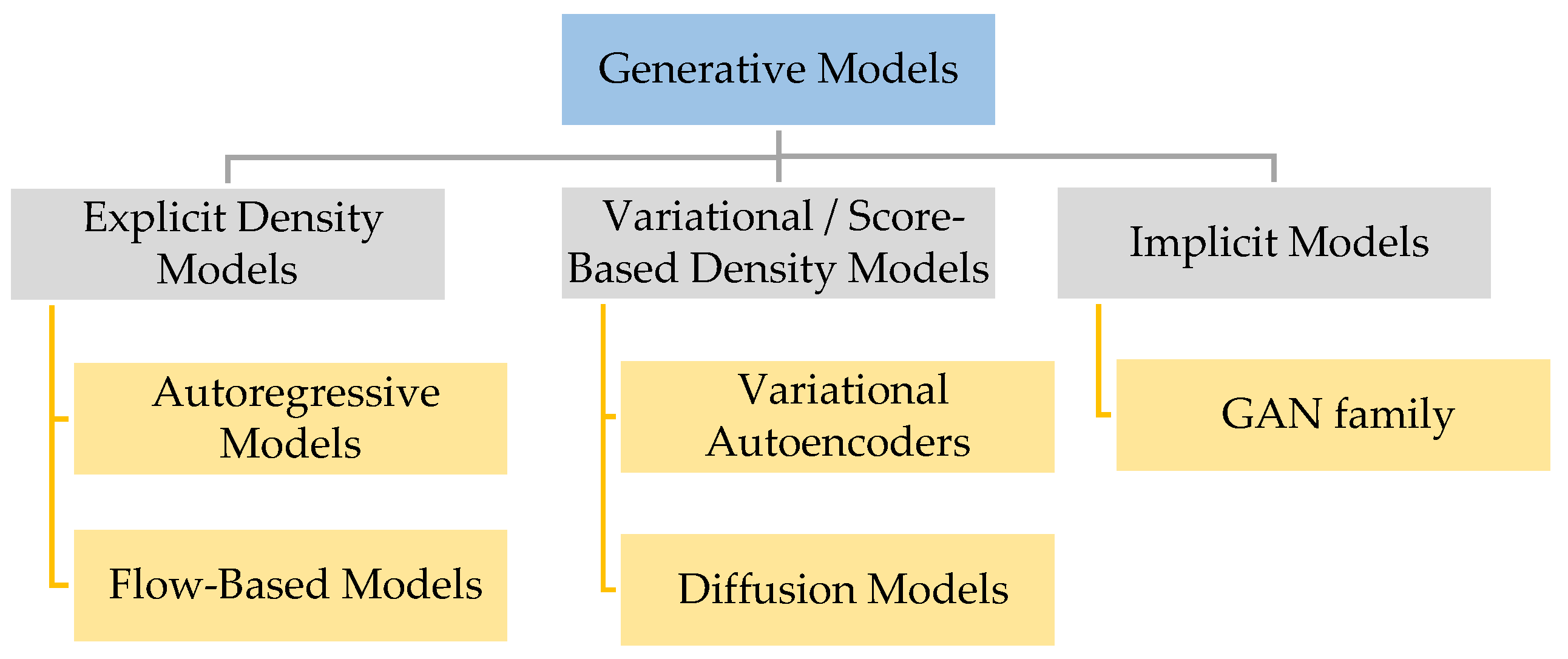
Figure 1. Taxonomy of Generative Models. This diagram organizes generative models into three principal families: explicit density models (which compute tractable likelihoods directly), variational and score-based density models (which optimize approximate or score-matching objectives), and implicit models (which learn to match distributions without explicit likelihood computation). Arrows indicate that diffusion and score-based models bridge variational inference and score-matching perspectives, while implicit models such as GANs can be combined with diffusion frameworks (e.g., Denoising Diffusion GANs) to form hybrid approaches.
Electronics 15 01293 g001
Figure 2. An Overview of Flow-Based Models.
Electronics 15 01293 g002
Figure 3. An overview of VAE architecture.
Electronics 15 01293 g003
Figure 4. An Overview of GAN architecture. The green and orange boxes denote the generator and discriminator networks, respectively. Black arrows indicate forward data flow and the pink arrow indicates backpropagation for generator updates.
Electronics 15 01293 g004
Figure 5. An Overview of Forward Diffusion and Reverse Diffusion. Beige circles denote sample states at different timesteps. The blue shaded area marks the diffusion stage. Solid arrows represent the forward noising process q ( x t x t 1 ) , while dashed arrows represent the reverse denoising process p ( x t 1 x t ) .
Electronics 15 01293 g005
Figure 6. An overview of DDPM. The top row illustrates the forward diffusion process from X 0 to X T , where beige circles denote sample states at different timesteps and blue arrows indicate the diffusion flow, with the blue dotted segment representing intermediate steps. The yellow line and arrow denote preprocessing that routes the noisy sample X T into the network. In the middle, blue blocks represent network layers and blue dashed lines indicate skip connections. The green blocks denote fully connected layers, while pink dashed arrows represent timestep conditioning by T . On the right, pink boxes show intermediate outputs from Y T to Y 0 , and green arrows indicate the reverse denoising progression.
Electronics 15 01293 g006
Figure 7. An overview of Latent Diffusion Architecture.
Electronics 15 01293 g007
Figure 8. An overview of Stable Diffusion Architecture, a Latent Diffusion Model trained with text conditioning. The beige panel on the left denotes pixel space, where the input image x   is encoded by the green encoder E into the latent representation z , and the reconstructed image x ~   is obtained through the green decoder D . The blue panel in the center denotes the latent space, where diffusion is performed on latent variables from z   to z T ; yellow blocks indicate latent states, solid black arrows show the main data flow, and curved arrows indicate the iterative noising and denoising steps. Inside the latent space, the purple U-Net blocks represent the denoising network ϵ θ , the gray QKV boxes denote attention modules, and the gray dashed arrows indicate information flow across U-Net stages. The gray panel on the right denotes the conditioning module, where orange, purple, blue, and light gray boxes represent semantic map, text, representation, and image-based conditioning inputs, respectively, which are processed by the green conditioning network τ θ and injected into the denoising U-Net.
Electronics 15 01293 g008
Figure 9. (a) DiT Architecture: Conditional latent models process patches. (b) DiT blocks with adaptive layer norm, (c) cross-attention, and extra tokens; (d) adaptive layer norm performs best.
Electronics 15 01293 g009
Figure 10. Consistency models map any point on a PF-ODE trajectory to its origin. Adapted from [47].
Electronics 15 01293 g010
Figure 11. Progressive Distillation (Multi-step to Few-step). Adapted from [49].
Electronics 15 01293 g011
Figure 12. Five-dimensional taxonomy of diffusion models along representation space, forward process, reverse parameterization, sampling strategy, and conditioning mechanism.
Electronics 15 01293 g012
Figure 13. Noise Domain.
Electronics 15 01293 g013
Table 1. VAE Variant.
VariantConditioning/StructureLatent RepresentationArchitectural ModificationRepresentative Use CasesKey Advantage
CVAE [10]Uses auxiliary conditions (e.g., class labels, side information) in both encoder and decoderContinuous latent distribution conditioned on inputsEncoder and decoder take conditional inputs; optimize conditional ELBOClass-conditional generation, controlled synthesisEnables guided generation using auxiliary information
VGAE [9]Designed for graph-structured data; node features are encodedContinuous latent embeddings per graph nodeGCN layers in encoder; inner-product decoderLink prediction, graph embeddingCaptures relational and topological structure
VQ-VAE [11]Unconditional or conditional via codebook guidanceDiscrete codebook of latent embeddingsEncoder outputs nearest codebook vector; commitment lossesHigh-fidelity image/audio generation, tokenized representationsDiscrete latent codes improve representation and alleviate posterior collapse.
Table 2. Representative GAN Variants and Their Core Modifications.
GAN VariantCore ModificationPrimary ApplicationKey Features
BicycleGANAdds a bijection between output and latent space to prevent models from generating few repetitive samples.Diverse image-to-image translationMaps output back to latent space; avoids repetitive sample generation [15]
BigGANExpands model size with increased batch size and layer width, adding skip connections and orthogonal regularization.High-fidelity class-conditional synthesisLarge model size; improved performance with skip connection; orthogonal regularization [16]
CycleGANWorks in a cyclic manner, mapping input to output and vice versa, supporting paired and unpaired images.Unpaired image-to-image translationCycle consistency loss; mapping between paired/unpaired images; mean squared error calculation [14]
DCGANsUses convolutional layers to generate realistic images, effective in unsupervised learning.General image synthesisConvolutional layers in both generator and discriminator; hierarchical image representation learning [17]
FRVSR-GAN (Frame Recurrent VSR-GAN)Designed for video super-resolution, generating high-quality frames sequentially using a recurrent architecture.Video super-resolutionFrame-to-frame dependency; recurrent neural network architecture for video frames.
GauGANDeveloped by NVIDIA, generates images based on text, semantic segmentation, sketches, and style.Semantic image synthesisMulti-input capability; supports interactive sketch-based generation [18]
InfoGANMaximizes mutual information to learn interpretable features, separating style from content (e.g., writing style from digit shape).Disentangled representation learningMutual information maximization; interpretable latent variables [19]
LayoutGANGenerates object layouts with multiple self-attention layers on 2D planes to create semantic relationships.Graphic and layout generationMulti-layer attention for layout generation; rendering layer for layout [20]
MaskGANMaps semantic segmentation to target images, allowing interactive manipulation of segmentation maps to produce new images.Semantic editing and manipulationDense Mapping Network and Editing Behavior Simulator; interactive manipulation of segmentation maps [21]
OC-GANAddresses complex scenes with multiple objects, avoiding spurious or overlapping object generation using bounding boxes.Multi-object scene synthesisObject-centric approach; bounding box generation and management [22]
SAGAN (Self-Attention GAN)Uses self-attention mechanisms to capture long-range dependencies, allowing fine-grained details in high-resolution images.High-resolution synthesisSelf-attention layers; long-range dependency modeling for detailed image consistency [23]
SN-GAN (Spectral Normalization GAN)Resolves gradient vanishing/exploding and model collapse issues using spectral normalization.Stable adversarial trainingSpectral normalization for stability; improved training process [24]
SRGANEnhance low-resolution images to high-resolution ones by leveraging adversarial training and perceptual loss, producing photo-realistic detailsSuper-resolutionPerceptual loss, realistic outputs, texture preservation, adversarial training, and versatile applications [25]
StyleGANEmploys an alternative generator architecture inspired by style transfer, with progressive training and mixing regularization to improve image generation quality.High-fidelity image synthesisProgressive growing, style vectors from latent variables, mixing regularization [13]
VQ-GAN (Vector Quantised GAN)Combines Vector Quantized approach with GAN to produce higher-quality images with reduced noise.High-resolution synthesisVector quantizer with discrete codebook vectors; noise reduction and object constraints [26]
Table 3. Comparative Summary of Generative Model Paradigms.
CriterionVAEGANFlowDiffusion
LikelihoodVariational lower bound (ELBO)Not applicable (implicit)Exact (change in variables)Variational bound or score matching
Training StabilityStable; straightforward optimizationProne to mode collapse and instabilityStable; bijective constraintStable; simple denoising objective
Sample QualityModerate; often blurryHigh; sharp and realisticModerate to highHigh; comparable or superior to GANs
Sampling SpeedFast (single forward pass)Fast (single forward pass)Fast (single forward pass)Slow (iterative; 10 to 1000 steps)
Mode CoverageGood but may underfitProne to mode droppingFull (bijective)Excellent coverage
ControllabilityLatent interpolationLimited without auxiliary lossesInvertible; supports editingStrong (CFG, ControlNet)
ScalabilityModerateHigh with progressive trainingLimited by invertibilityHigh with latent space formulations
Typical ApplicationsRepresentation learning, anomaly detectionImage synthesis, style transferDensity estimation, exact inferenceImage/video synthesis, inpainting, conditional generation
Table 4. Mapping Diffusion Models to the taxonomy axes.
ModelRepresentation SpaceForwardReverse ParameterizationSampling StrategyConditioning Mechanism
DDPMPixelVPNoiseStochasticNone
DDIMPixelVPNoiseDeterministicNone
Score-SDEPixelVEScoreODE/SDEOptional
LDMLatentVPNoiseDDIM/ODEText
Stable DiffusionLatentVPNoiseDDIM + CFGText
DiTLatent/PatchVPNoise/VelocityODEText
ControlNetLatentVPNoiseDDIMStructural
Consistency ModelPixel/LatentVP/VEScore/DataSingle-step/Few-step ODEOptional/CFG
Progressive DistillationPixel/LatentVPNoiseFew-step Distilled SamplerSame as base model
VP: Variance Preserving; VE: Variance Exploding; CFG: Classifier-Free Guidance.
Table 5. Recommended Diffusion Model Design Choices by Noise Type.
Noise TypeDomainDistributionRecommended Forward ProcessPreprocessing Strategy
Photon shot noiseLow light photographyPoissonVariance Exploding (VE) SDEVariance stabilizing transform (e.g., Anscombe)
Speckle noiseMedical ultrasoundRayleigh/multiplicativeVE SDE with adapted scheduleLog transform; bilateral filtering for smoothing
Gaussian sensor noiseGeneral photographyGaussianVariance Preserving (VP) SDE (standard DDPM)Standard normalization
Compression artifactsJPEG images, web imagesStructured/blockyVP SDEDCT domain denoising as preprocessing
Thermal/read noiseHigh ISO, infraredGaussian mixtureVP or EDM parameterizationBM3D or wavelet denoising as preprocessing
Atmospheric distortionRemote sensing, satelliteNon Gaussian (complex)VE SDE or EDMWavefront correction; variational filtering
Table 6. Comparison of External Denoising Techniques Relevant to Diffusion Pipelines.
TechniqueKey IdeaAdvantagesLimitationsTypical Use Cases (with Diffusion Models)
Mean FilterReplaces each pixel with the average value of its local neighborhood.
  • Simple to implement
  • Reduces random noise
  • Blurs edges
  • Not robust to outliers
Rarely used; coarse smoothing in early preprocessing.
Median FilterReplaces each pixel with the median value of its local neighborhood.
  • Good at removing salt-and-pepper noise
  • Preserves edges better than mean filter
  • More computationally expensive than mean filter
  • Not ideal for all noise types
Preprocessing for corrupted training data with impulse noise.
Non-Local Filtering (BM3D)Groups similar blocks (patches) into 3D arrays and applies collaborative filtering.
  • State-of-the-art performance
  • Preserves fine details and textures
  • Computationally intensive
  • Relies on accurate block-matching
Optional post-processing for fine-detail preservation in high-fidelity outputs.
Transform Domain Denoising
(e.g., DCT, Fourier)
Transforms the image to a frequency domain, then thresholds or smooths high-frequency coefficients.
  • Effective for structured or periodic noise
  • Reduces compression artifacts
  • Risk of oversmoothing delicate details
  • Requires careful threshold selection
Removing banding or ringing artifacts in post-processing.
Bilateral FilteringUses spatial and intensity differences to weight neighboring pixels, preserving edges while smoothing.
  • Edge-preserving
  • Avoids halo artifacts around edges
  • Slower compared to linear filters
  • Parameter tuning (spatial/intensity sigma) can be tricky
Post-processing when edge fidelity is visually important.
Wavelet Transform DenoisingDecomposes image into wavelet coefficients; thresholds high-frequency coefficients to reduce noise.
  • Multi-scale analysis
  • Preserves edges well
  • Adaptable thresholding
  • Choice of wavelet family
  • Threshold setting can be non-trivial
High-resolution domains (e.g., medical imaging, remote sensing) after generation.
Denoising Autoencoders (DAE)Neural networks trained to map noisy inputs to clean outputs, learning complex noise patterns.
  • Highly flexible
  • Learns data-specific noise characteristics
  • Can handle high-dimensional data (images/videos)
  • Requires large, diverse training data
  • Possible overfitting if noise distributions differ from training conditions
Post-processing in domain-specific pipelines (e.g., scientific visualization, medical content).
Table 7. Diffusion Model Use Cases, Key Architectural Features, and Evaluation Metrics.
Use CasePreferred Architecture (s)Conditioning/Post-ProcessingKey Metrics for Evaluation
Movie & Scene GenerationStable Diffusion,
Latent Diffusion [63,64]
BM3D,
Non-local filtering
PSNR,
SSIM
Recreational ContentText-Guided Diffusion [31,32,65]Mean/Median filteringVGG-based perceptual similarity
Robotics,
Remote Sensing
DDPM [66,67],
Latent Diffusion [68,69,70,71,72]
Robust detail-preserving methodsSSIM, Temporal Consistency
Educational ContentDDPM, Latent Diffusion [73]Transform domain denoisingSSIM, Perceptual Similarity
Table 8. Curated list of Datasets Used in Diffusion and Generative Models.
CategoryDatasetImages/FrameDescriptionUse Case
General Image Generation BenchmarksBSDS500 [74] 500 imagesBoundary detection dataset, beneficial for edge detection and segmentation applications.Edge detection, boundary analysis
CIFAR-10 [75]60,000 images (50 k train, 10 k test)Low-resolution (32 × 32) natural images across 10 object classes; widely used as a benchmark dataset for generative modeling and diffusion modelsBenchmarking diffusion models, low-resolution image generation
Imagenet [76]14 millionWidely used image classification dataset covering a broad spectrum of object categories.Image classification, foundational model training
LSUN [77]1 million+High-quality images for large-scale scene understanding, covering bedrooms, churches, outdoor scenes, etc.Large-scale scene generation
Places365 [78]1.8 millionScene dataset covering various place types, such as landscapes, urban areas, and indoor scenes.Scene generation, place recognition
High-Fidelity Image GenerationBigGAN [16]14 millionDataset specifically curated for GAN training, covering multiple high-quality categories.High-fidelity image generation
CelebAMask-HQ [79]~30,000High-resolution face images with facial segmentation masks.High-fidelity face generation
DIV2K [80]1000 high-resolution imagesHigh-quality 2K resolution images designed for super-resolution tasks, containing diverse natural scenes with fine detailsSuper-resolution, high-fidelity image generation
FFHQ (Flickr-Faces-HQ) [13]70,000High-quality dataset of human faces for training and evaluating face generation models.Face generation, high-resolution synthesis
Scene UnderstandingADE20K [81]25,574 (train), 2000 (val)Used for segmentation and object detection.Scene segmentation, object detection
COCO-Stuff [82]118 k (train), 5 k (val)Scene understanding tasks, including segmentation, object detection, and image captioning.Scene generation, object detection
HICO-DET [83]15,963 (train), 4034 (val)Focuses on detecting Human–Object Interactions (HOI).Human–object interaction modeling
MS-COCO [84]328 kObject Detection, Segmentation, Captioning, and Keypoint detection dataset.Object detection, image captioning
OpenImages [85]~9 millionContains images annotated with object bounding boxes, segmentation masks, and visual relationships.Object detection, segmentation, relationship modeling
PASCAL VOC [86]11,530 imagesClassic dataset for object detection and segmentation in general visual categories.Object detection, segmentation
MultimodalCC3M [87]3.3 millionImage–caption pairs, designed for image captioning model training and evaluation.Image captioning, multimodal training
CC12M [88]12 millionImage–text pairs for vision and language pre-training.Vision–language pre-training
Flickr [89]70,000 (train), 10,000 (val)Benchmark for sentence-based image description.Image captioning, sentence-based image tasks
LAION-5B [90]5.85 billionLarge-scale image–text dataset, open source, for next-generation multimodal model training.Text-to-image/video generation, multimodal training
NUS-WIDE [91]269,648 imagesImage–text pairs with diverse tags, ideal for text-to-image generation tasks with varied scene categories.Text-to-image generation, image tagging
Visual Genome [92]~108 kRegion descriptions and Q&A pairs associated with WordNet synsets for multimodal tasks.Text-to-image generation, Q&A
Video GenerationCharades [93]9848 videosReal-world video dataset for action recognition and captioning, covering complex activities and interactions.Human activity synthesis, video Q&A
DAVIS 2017 [94]90 video sequencesHigh-quality video dataset with segmentation masks, useful for video segmentation tasks.Video segmentation, motion tracking
HMDB51 [95]~7000 videosVideo dataset containing clips from various action categories, such as sports and human interactions.Human action modeling, video generation
Kinetics-700 [96]~650,000 videosVideo action recognition dataset with multiple classes, useful for generating human activity sequences.Human action generation, video synthesis
Sports1M [97]~1 millionVideo dataset with sports-related content, tagged with metadata about activity types.Sports action generation, video recognition
VaTeX [98]41,250 videos, 825,000 captionsA large-scale multilingual video-and-language dataset, containing captions in both English and Chinese.Video captioning, multilingual video research
Vimeo90K [99]90,000 video clipsVideo dataset for tasks like frame interpolation and video super-resolution.Video frame interpolation, enhancement
YouTube-8M [100]6.1 million video segmentsVideo dataset with audio–visual content across a wide range of categories.Video generation, multimodal tasks
3D and Scene Generation3D Front [101]-Large-scale synthetic indoor scenes with professionally designed layouts.Interior design, 3D scene generation
BlenderBot 3D [102] 10 k scenes3D dataset for virtual environment generation, suitable for training 3D-aware generative models.3D scene generation, virtual simulations
MatterPort [103]4939 (train), 456 (val)RGB-D dataset for indoor scene understanding with 3D layouts.Indoor scene understanding, VR/AR applications
ModelNet [104]9843 (train), 2468 (val)Contains synthetic object point clouds for 3D object recognition.3D object recognition
OASIS [105]9664 (train), 1120 (val)Large-scale dataset for single-image 3D reconstruction in wild settings.3D single-image reconstruction
RPLAN [106]118 kDensely annotated real residential floor plans.Architectural layout and floor plan generation
ScanNet [107]1201 (train), 312 (val)Instance-level indoor RGB-D data with 2D and 3D annotations.Indoor scene understanding, 3D object recognition
ShapeNet [108]100,000+Large-scale dataset of 3D shapes, used for 3D object and scene understanding.3D shape generation and recognition
SUNCG [109]53,860Large-scale synthetic 3D scenes with dense volumetric annotations.3D scene generation, virtual environment modeling
YouTube 3D [110]47,125 (train), 1525 (val)3D vertex coordinates derived from YouTube videos.3D object tracking, video synthesis
Autonomous DrivingCityscapes [111]5000Focuses on semantic segmentation of urban street scenes.Autonomous driving, urban scene generation
Indian Driving Dataset (IDD) [112] ~10,000Road scene understanding dataset for unstructured environments.Road scene generation, autonomous driving
KITTI [113]22,000Street-level images with 3D bounding boxes for autonomous driving and object detection tasks.Autonomous driving, street scene generation
Synscapes [114]-Synthetic dataset for street scene parsing, created using photorealistic rendering techniques.Street scene generation, autonomous driving
YCB [115]80,000 (train), 5000 (val)RGB-D scans for robotic manipulation, with high-resolution object meshes.Robotics, manipulation training
Depth and GeometryDIODE [116]25,458 (train), 771 (val)High-resolution color images for indoor and outdoor scenes.Depth estimation, indoor–outdoor scene understanding
MegaDepth [117]130 kDepth maps of complex scenes, valuable for depth-aware generation tasks.Depth map generation, 3D modeling
Specialized DatasetsCLEVR-G [118]10,000 (train), 10,000 (val)Visual Question Answering dataset with 3D-rendered object images.Visual Q&A, synthetic object generation
ColorMNIST [119]8000 (train), 8000 (val)Synthetic binary classification task derived from MNIST.Simple classification tasks
DeepFashion [120]~800,000Large-scale clothing dataset for tasks such as garment segmentation and clothing category classification.Clothing generation, virtual try-on
Fashion-MNIST [121]70,000 imagesDataset for clothing item classification, useful for generative model testing in the fashion domain.Fashion synthesis, classification
Table 9. Comparative Overview of Key Performance Evaluation Metrics.
MetricKey IdeaAdvantagesLimitationsTypical Use Cases (in Diffusion Models)
PSNR (Peak Signal-to-Noise Ratio)Measures pixel-level fidelity using logarithmic scale of inverse MSE between generated and ground truth images.Simple to compute; widely used in denoising/restoration tasks.Poor correlation with human perception; not meaningful for generative sampling.Used in reconstruction tasks (e.g., super-resolution, inpainting) where ground truth is known.
SSIM/MS-SSIM (Structural Similarity Index)Compares structure, contrast, and luminance between ground truth and generated images; MS-SSIM does so at multiple resolutions.Better alignment with perceptual quality than PSNR; sensitive to structural distortions.Still a handcrafted metric; may miss semantic mismatches or large shifts.Used in pixel-level tasks with structural expectations (e.g., denoising, enhancement).
Perceptual SimilarityEvaluates feature-level differences using a pre-trained network (e.g., VGG), aiming to mimic human visual perception better than pixel-based comparisons.- Focuses on semantic and structural aspects.
- Generally aligns more closely with human perception than SSIM or PSNR.
- Less sensitive to small pixel shifts.
- Depends on choice of pre-trained network (domain mismatch can affect results).
- Computationally heavier (feature extraction).
- Does not measure coverage of entire data distribution (pairwise only).
- Ideal for tasks requiring photo-realism or style consistency (e.g., artistic generation, super-resolution).
- Useful for iterative refinement of diffusion outputs.
MOS (Mean Opinion Score)Averages human ratings of visual quality across evaluators.Captures real human perception; useful in creative domains.Expensive, time-consuming, prone to bias.Used in user-facing applications (e.g., art, UI, entertainment).
Fréchet Inception Distance (FID)Distribution-based metric: compares means and covariances of real vs. generated images in a deep feature space (Inception v3).Captures both quality and diversity; widely adopted benchmark.Assumes Gaussian distribution; sensitive to batch size and extractor quality.Standard metric for generative image models (unconditional, text-conditioned).
FVD (Fréchet Video Distance)Extension of FID to video: compares temporal feature distributions using I3D network.Captures temporal consistency; correlates well with human realism judgments.Requires large sample size; assumes Gaussian statistics.Standard for generative video evaluation (e.g., text-to-video diffusion).
IS (Inception Score)Measures image recognizability and class diversity using pre-trained Inception classifier.No need for real data; fast to compute.Poor correlation with human judgment; insensitive to distribution mismatch.Legacy metric; sometimes reported alongside FID for completeness.
Kernel Inception Distance (KID)Uses a non-parametric MMD in the Inception feature space to compare real vs. generated distributions, avoiding Gaussian assumptions.- More flexible than FID (no Gaussian assumption).
- Can be more robust with certain data distributions.
- Like FID, it looks at distribution coverage.
- Potentially more computational than FID (kernel computations).
- Still depends on a feature extractor (Inception v3).
- Requires real data for comparison.
- Alternative or complement to FID when data distribution does not fit Gaussian assumptions.
- Used in high-quality generative tasks to confirm distribution alignment.
LPIPS (Learned Perceptual Image Patch Similarity)Measures perceptual similarity in deep feature space using pretrained models like VGG or AlexNet.Strong perceptual correlation; captures high-level textures and semantics.Dependent on network architecture; does not assess distribution-wide realism.Common for assessing perceptual quality in generative tasks (e.g., image synthesis, editing).
Table 10. Use Cases and Architecture Connections.
ModelDatasetPSNRSSIMPerceptual SimilarityFIDISKIDLPIPS
DDPMCIFAR-1039.07220.99880.02342.58839.1185 ± 0.7170−0.00056 ± 0.0000400.0006
DDPMDIV2K5.01020.0029 (MS: 0.0120)184.109414.75131.0077 ± 0.00210.1066 ± 0.0008 (mean ± std)0.8485
Stable Diff.CIFAR-107.590.00990.1181562.16951.2171 ± 0.01470.7698 ± 0.00000.9602
Stable Diff.DIV2K9.50.140120.0151365.33832.3525 ± 0.23190.3239 ± 0.00000.789
Latent Diff.CIFAR-108.32450.03070.2108147.99281.1469 ± 0.0045−0.0005 ± 0.00010.1875
Latent Diff.DIV2K6.690.00440.0662426.471.0000 ± 0.00000.3720 ± 0.00110.8175
Disclaimer/Publisher’s Note: The statements, opinions and data contained in all publications are solely those of the individual author(s) and contributor(s) and not of MDPI and/or the editor(s). MDPI and/or the editor(s) disclaim responsibility for any injury to people or property resulting from any ideas, methods, instructions or products referred to in the content.