Article

Large-Signal Stability Enhancement for FIS: Criterion-Based Parameter Optimization and Power Differentiation Feedforward Control

Department of Electrical Engineering, Electrical Engineering College, Guizhou University, Guiyang 550025, China
*
Author to whom correspondence should be addressed.
Electronics 2026, 15(6), 1283; https://doi.org/10.3390/electronics15061283
Submission received: 6 February 2026 / Revised: 10 March 2026 / Accepted: 16 March 2026 / Published: 19 March 2026
(This article belongs to the Section Power Electronics)

Abstract

Flexible interconnection systems (FISs) improve distribution flexibility, yet they remain vulnerable to pronounced nonlinear instability and potentially severe DC-link voltage collapse during large disturbances such as constant power load (CPL) surges. Conventional linear control methods are often unable to prevent deep transient voltage dips under these conditions. To address this issue, this paper proposes a novel large-signal stability criterion based on mixed potential function (MPF) theory. Unlike conventional Lyapunov-based approaches, the proposed formulation explicitly incorporates the dynamics of the DC capacitor, thereby enabling the derivation of a closed-form stability boundary. On this basis, the proportional gains of the outer voltage loop are first optimized to guarantee an adequate static stability margin. Subsequently, a power differentiation feedforward control strategy is developed. Rather than passively counteracting transients, the proposed method dynamically adjusts the DC voltage reference according to the rate of change in power, thereby actively reshaping the transient trajectory. In this way, the simple PI control framework is preserved while avoiding the heavy computational burden associated with advanced methods such as model predictive control. Simulation results show that the proposed strategy increases the permissible CPL step power by 8.7%, from 92 kW to 100 kW. Moreover, under severe load surges and weak grid conditions, the method prevents voltage collapse and maintains the transient trajectory above the practical 600 V safe-operation threshold. This computationally efficient strategy significantly improves the robustness and continuity of operation of practical FISs.

1. Introduction

With the ongoing global energy transition and the increasing penetration of renewable energy sources such as wind and solar power, modern power systems are experiencing pronounced stochastic fluctuations on the load side and a continuously rising share of power electronic interfaces [1,2]. Flexible interconnection systems (FISs), which employ power electronic converters to realize flexible interconnection and dynamic energy dispatch among multiple regional grids, have, therefore, become key equipment for enhancing distribution network flexibility and renewable energy accommodation [3,4]. However, under large disturbances such as sudden load surges, FISs are prone to instability and even voltage collapse. Traditional small-signal stability analysis, which relies on linearized models, is inherently limited by local linearization and, therefore, cannot accurately capture the nonlinear dynamic behavior or instability mechanisms of the system under large disturbances [5,6]. Consequently, rigorous large-signal stability analysis of FISs, together with corresponding parameter optimization and stability-oriented control design, is essential for ensuring the secure and stable operation of modern power systems.
Unlike small-signal analysis, large-signal stability analysis must explicitly account for the strong nonlinearity of the system. Existing large-signal stability analysis methods for power-electron-dominated systems mainly include the Lyapunov direct method, the Takagi–Sugeno (T-S) fuzzy model approach, and mixed potential function (MPF) theory [7,8,9]. The Lyapunov direct method is theoretically rigorous; however, constructing an appropriate Lyapunov function often depends heavily on experience, and it is difficult to generalize to high-order complex systems [10]. Although T-S fuzzy model-based methods can effectively approximate nonlinear systems, their computational burden increases rapidly with model order because of the “curse of dimensionality” [11]. By contrast, the MPF framework provides a systematic, topology-oriented approach for constructing the system energy function by explicitly combining the stored energy of dynamic components with the dissipative content of resistive elements. Because the resulting MPF is closely aligned with the physical characteristics of the circuit, it can generally provide a less conservative and more physically interpretable stability criterion. Rather than relying on the geometrically complex estimation of the region of attraction required by many classical Lyapunov approaches, MPF theory can yield explicit algebraic parameter boundaries. This feature is particularly attractive for controller parameter design because it offers a tighter and more practical characterization of the safe operating region [12,13,14].
Building on these methodological advantages, many studies have applied MPF theory to specific power electronic systems. In [15], the voltage source converter (VSC) was simplified as a DC circuit with a controlled current source, and an MPF-based large-signal stability criterion was derived. In [16], the load converter was modeled as a constant power load (CPL), the MPF of the cascaded system was established, and the influence of control parameters on stability was analyzed. To improve model fidelity, [17] further represented the load side as an equivalent controlled source. In [18], the cascaded system formulation was combined with the VSC model to obtain a stability criterion for VSC-HVDC systems, whereas [19] derived the MPF for modular multilevel converters (MMCs) and introduced a conservative correction factor to reduce over-conservatism. Nevertheless, existing criteria are often derived from overly simplified models, which would compromise their accuracy and limit their ability to reveal stability relationships over a broad parameter range.
With regard to large-signal stability enhancement, existing studies mainly focus on advanced nonlinear control algorithms, hardware modification, and refinements of conventional control schemes. Advanced nonlinear methods—such as model predictive control (MPC), sliding mode control (SMC) [20], and backstepping [21]—can deliver excellent dynamic performance during severe transients. However, their large-scale industrial deployment is still constrained by the need for accurate mathematical models and substantial real-time computational resources. Alternatively, adding auxiliary hardware, such as active capacitors [22], can significantly improve stability but at the expense of increased system volume and cost. Improvements within the classical control framework also face strict physical limitations. For example, transient path optimization [23] has difficulty coping with stochastic disturbances in real time, while virtual capacitor strategies [24] and complex feedforward loops [25] are fundamentally limited by the converter overcurrent margin. Likewise, improved droop control methods [26,27] depend strongly on the availability of sufficient power reserve at neighboring terminals in networked systems.
Therefore, bridging theoretical stability analysis and practical engineering implementation without relying on computationally intensive algorithms or costly additional hardware remains an important challenge. Translating stability criteria into actionable controller design is especially important in this context. Parameter optimization based on the MPF stability boundary offers a systematic route for selecting proportional–integral (PI) gains that improve system robustness. In addition, by introducing a power differentiation feedforward control scheme that dynamically reshapes the DC voltage reference according to the measured rate of change in power, the active disturbance rejection capability of the system can be further strengthened.
Accordingly, this paper proposes an economical, practical, and margin-independent stability enhancement strategy for FISs under severe large-signal disturbances. The main contributions and novelties of this study are summarized as follows:
  • A comprehensive nonlinear model of the FIS is established, and an improved MPF-based stability criterion is derived by explicitly incorporating the dynamic characteristics of the DC-side capacitor. The resulting criterion provides a more accurate stability margin than conventional MPF formulations.
  • A systematic parameter optimization method is developed to connect the abstract stability criterion with practical PI controller tuning, thereby improving large-signal stability without additional hardware cost.
  • A novel power differentiation feedforward control strategy is proposed. By sensing the power rate of change in real time, the strategy dynamically reshapes the voltage reference during transient events, effectively suppressing voltage fluctuations and enhancing large-signal stability under severe grid and load disturbances.
  • Extensive simulations verify the effectiveness of the proposed strategy and demonstrate superior performance over conventional methods in both stability range and transient recovery.
The remainder of this paper is organized as follows. Section 2 describes the system topology and establishes the basic mathematical model of the two-terminal flexible interconnection system. Section 3 constructs the mixed potential function, derives the large-signal stability criterion, and presents the parameter optimization method. Section 4 details the proposed power differentiation feedforward control strategy. Section 5 presents comprehensive simulation results to validate the effectiveness of the proposed method. Section 6 discusses the applicability of the proposed strategy to multi-terminal systems with droop control. Finally, Section 7 concludes the paper.

2. System Description and Mathematical Modeling

The topology of a typical two-terminal VSC-based flexible interconnection system (FIS) used in distribution networks is shown in Figure 1. The FIS consists of two voltage source converters (VSCs) sharing a common DC-link capacitor. The rectifier is located at the sending end and adopts constant DC voltage control to regulate the DC bus voltage, whereas the inverter is located at the receiving end and operates under constant power control to inject power into the AC grid.
In Figure 1, the main variables and parameters are defined as follows: usabc denotes the grid voltage on the rectifier side, and iabc represents the rectifier grid current; Lr and Rr are the equivalent inductance and resistance of the AC-side line, respectively; Ls and Rs denote the filter inductance and its equivalent series resistance, respectively; Prec denotes the active power absorbed by the rectifier from the grid; uabc is the AC-side voltage of the rectifier; udc is the DC bus voltage; and Cdc is the DC-link capacitance. In addition, Pinv and usabc_inv denote the inverter output power and the inverter-side grid voltage, respectively.
According to Figure 1, the Kirchhoff voltage law (KVL) for the AC side of the FIS can be written as
u s a b c u a b c = L f d i a b c d t + R f i a b c
where Lf = Lr + Ls and Rf = Rr + Rs are the lumped equivalent inductance and resistance on the AC side, respectively. By applying the amplitude-invariant transformation to the variables in (1), the model can be transformed into the synchronous dq0 rotating reference frame. In this paper, the d-axis is aligned with the grid voltage vector, and the d-axis leads the q-axis by 90°. Accordingly, usd ≈ Um and usq ≈ 0, and the mathematical model in the dq frame can be obtained as
u s d u d = L f d i d d t + R f i d ω L f i q u s q u q = L f d i q d t + R f i q + ω L f i d
where usd, ud, and id denote the d-axis components of usabc, uabc, and iabc, respectively, whereas usq, uq, and iq denote the corresponding q-axis components. ω represents the grid angular frequency.
The active power input to the rectifier is given by
P r e c = 3 2 u d i d + u q i q
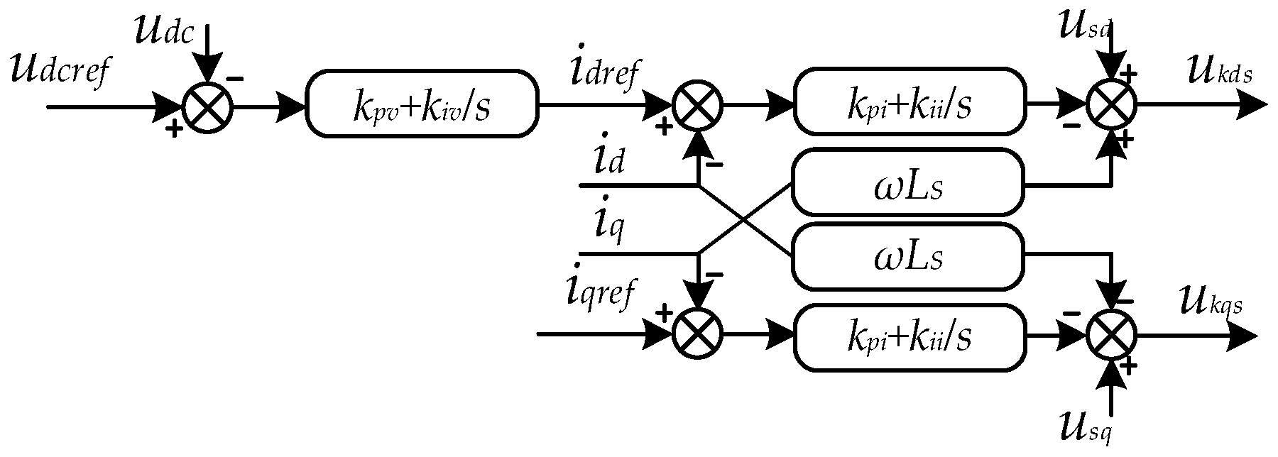
The control block diagram of the rectifier in the FIS is shown in Figure 2. The rectifier adopts constant DC voltage control to support the DC bus voltage. In Figure 2, udcref denotes the DC voltage reference, and udc is the measured DC bus voltage; idref and iqref are the reference values of the AC-side current components id and iq, respectively; ukds and ukqs represent the reference values of the converter output voltage components ud and uq, respectively.
As shown in Figure 2, the outer voltage loop regulates the DC voltage to its nominal value and generates the d-axis current reference for the inner loop. The corresponding control law is expressed as
i d r e f = k p v u d c r e f u d c + k i v u d c r e f u d c d t i q r e f = 0
Similarly, the current inner-loop controller can be expressed as
u k d s = u s d k p i i d r e f i d k i i i q r e f i q d t + ω L f i q u k q s = u s q k p i i q r e f i q k i i i q r e f i q d t ω L f i d
where ukds and ukqs are then processed by PWM modulation to generate the control signals for the rectifier.

3. Large-Signal Stability Analysis Based on MPF

3.1. Mixed Potential Function Theory

The mixed potential function (MPF) theory, proposed by R.K. Brayton and J.K. Moser in 1964, can be regarded as a generalized extension of the Lyapunov function method. It has been widely applied to the large-signal stability analysis of AC/DC systems containing constant power loads (CPLs). Brayton and Moser showed that, for nonlinear RLC circuits with different topologies, although the corresponding characteristic equations may vary, they can be represented in a unified mathematical form, expressed as
P ( i , v ) i = L d i d t P ( i , v ) v = C d v d t
where P denotes the mixed potential function (MPF) of the circuit; L represents the inductance in the circuit, and i is the corresponding inductor current; C denotes the capacitance, and v is the corresponding capacitor voltage. For a circuit with known parameters, the MPF can be employed to construct a Lyapunov-type energy function for assessing circuit stability. The MPF consists of a voltage potential function and a current potential function, and its standard form is given by
P ( i , v ) = A ( i ) + B ( v ) + ( i , γ v α )
where A(i) is the current potential function of the non-energy storage elements; B(v) is the voltage potential function of the non-energy storage elements; and the term (i,γv-α) is determined by the circuit topology. Once the MPF has been established, (6) can be used to verify its correctness. The construction procedure of the MPF can be summarized as follows:
  • Determine the potential functions of the non-energy storage elements in the circuit;
  • Calculate the energy associated with the capacitor elements;
  • Sum the values obtained in the previous two steps and obtain a standard form.
Based on the MPF model, the theory provides a theorem for large-signal stability analysis. Let Aii(i) denote the second-order partial derivative of the current potential function with respect to current and let Bvv(v) denote the second-order partial derivative of the voltage potential function with respect to voltage. Furthermore, let μ1 be the minimum eigenvalue of L−1/2Aii(i)L−1/2 and let μ2 be the minimum eigenvalue of C−1/2Bvv(v)C−1/2. If the condition
μ 1 + μ 2 δ δ > 0
is satisfied and, simultaneously, the auxiliary function P*(i,v) satisfies the condition
P * ( i , v ) = μ 1 μ 2 2 P ( i , v ) + 1 2 P i , L 1 P i + 1 2 P v , C 1 P v
as the state variables approach infinity, where Pi and Pv are the partial derivatives of the MPF P(i,v) with respect to current and voltage, respectively, then all system trajectories converge to the steady-state operating point, thereby ensuring stable operation of the system.

3.2. Mixed Potential Function of the Flexible Interconnection System

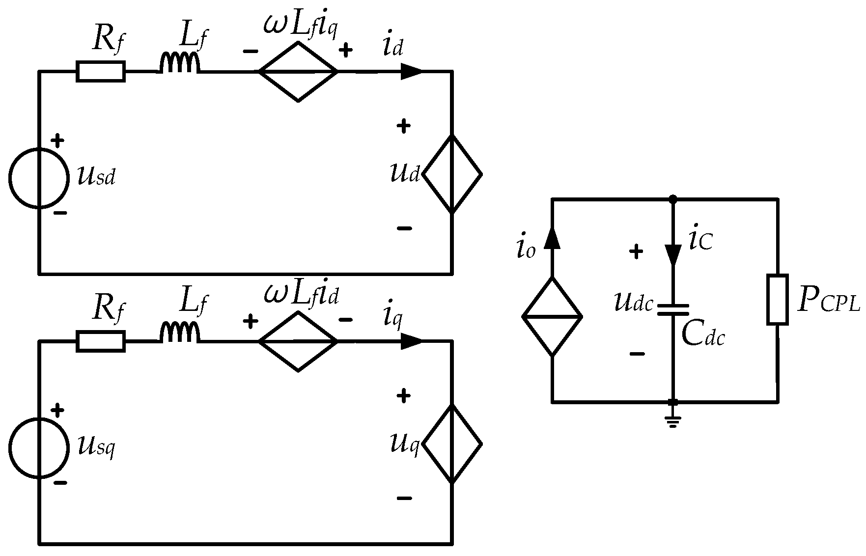
Based on the flexible interconnection system shown in Figure 1, a nonlinear average model is established, as shown in Figure 3. Since the inverter adopts constant-power control and its dynamic response is typically much faster than that of the rectifier, the inverter side can be simplified as a constant power load (CPL). Although practical inverters may reach current limits or experience control saturation during severe transients, thereby deviating from ideal CPL behavior, modeling the inverter as an ideal CPL represents the worst-case operating condition associated with the strongest negative impedance effect. Therefore, the stability boundary obtained under this assumption is inherently conservative and robust [19]. In Figure 3, io represents the DC output current, iC denotes the capacitor current, and PCPL is the inverter-side load power.
In Figure 3, iC denotes the current flowing through the DC-link capacitor Cdc. According to Figure 3, the potential function Pdc of the non-energy storage elements on the DC side of the FIS can be written as
P d c = u s d i d 1 2 R f i d 2 Γ u d d i d + Γ ω L f i q d i d + u s q i q 1 2 R f i q 2 Γ u q d i q Γ ω L f i d d i q + Γ u d c d i o Γ u d c d P C P L u d c
where Γ denotes the integration path. This path starts from the equilibrium point and extends from the equilibrium DC voltage udce to the state variable udc [28]. The term PC associated with the capacitor in the circuit is expressed as
P C = i o u d c + P C P L
By combining (10) and (11), the MPF P(i,v) of the DC side of the system is obtained as
P ( i , v ) = u s d i d 1 2 R f i d 2 Γ u d d i d + Γ ω L f i q d i d + u s q i q 1 2 R f i q 2 Γ u q d i q Γ ω L f i d d i q + Γ P C P L u d c d u d c Γ i o d u d c
Taking the partial derivative of the MPF in (12) with respect to voltage yields
P ( i , v ) i d = u s d R f i d + ω L f i q u d = L f d i d d t P ( i , v ) i d = u s q R f i q + ω L f i d u q = L f d i q d t P ( i , v ) u d c = P C P L u d c i o = C d c d u d c d t
It is evident that the derived potential function satisfies the condition in (6). Therefore, (12) represents the MPF of the system shown in Figure 1. Expressed in the standard form of the MPF, it yields
A ( i ) = u s d i d + 1 2 R f i d 2 + Γ u d d i d Γ ω L f i q d i q u s q i q + 1 2 R f i q 2 + Γ u q i q + Γ ω L f i d d i q B ( u d c ) = Γ i o d u d c + Γ P C P L u d c d u d c
Taking the second-order partial derivative of the voltage potential function in (14) yields
A i i ( i ) = R f + u d i d 0 0 R f + u q i q B v v ( u d c ) = P C P L u d c 2 i o u d c

3.3. Derivation of the Stability Criterion Based on MPF

Since the response speed of the current loop is significantly faster than that of the voltage loop, the dynamics of the inner current loop can be neglected, provided that the PI parameters are properly tuned. It is, therefore, assumed that the inner current loop tracks the reference generated by the outer voltage loop with negligible delay. Hence,
i d i d r e f i q 0
According to (15), evaluating the second-order partial derivative of the voltage potential function requires determining the partial derivative of the DC current io with respect to the DC voltage udc:
i o u d c = 1 u d c u d c i o u d c i o u d c
Neglecting the internal losses of power electronic devices and invoking the principle of power conservation, we obtain
u d c i o = 3 2 u d i d
Substituting the d-axis voltage equation in (2) into (18), the product udcio can be expressed as
u d c i o = 3 2 ( u s d i d R f i d 2 L f i d d i d d t )
Differentiating both sides of (19) with respect to udc yields
u d c i o u d c = 3 2 u s d i d u d c 2 R f i d i d u d c L f i d u d c d i d d t L f i d d i d d t u d c
Substituting (20) into (17), we obtain
i o u d c = 3 2 u d c u s d i d u d c 2 R f i d i d u d c L f i d u d c d i d d t L f i d d i d d t u d c i o u d c
According to (21), the partial derivative of io with respect to udc depends on ∂id/∂udc, did/dt, ∂(did/dt)/∂udc. Therefore, the explicit expression can be obtained by determining these three terms separately.
Based on the control law in (4), the time derivative of the current id is
d i d d t = k p v d u d c d t + k i v u d c r e f u d c
According to the constitutive relation of the DC-link capacitor, the capacitor current iC can be written as
i C = C d c d u d c d t
Combining this relation with Kirchhoff’s current law (KCL), the time derivative of the DC voltage udc is obtained as
d u d c d t = 1 C d c i o P C P L u d c
Substituting (24) into (22) yields
d i d d t = k p v C d c P C P L u d c i o + k i v u d c r e f u d c
Differentiating both sides of (25) with respect to udc, we obtain
d i d d t u d c = k p v C d c P C P L u d c 2 k p v C d c i o u d c k i v
Differentiating the control equation in (4) with respect to udc, the partial derivative of the d-axis current id with respect to udc is given by
i d u d c = k p v
Substituting (25), (26), and (27) into (21), the partial derivative of io with respect to udc is obtained as
i o u d c = 3 2 u d c u s d k p v 2 R f i d k p v L f k p v k p v C d c P C P L u d c i o + k i v u d c r e f u d c 3 2 u d c L f i d k p v C d c P C P L u d c 2 k p v C d c i o u d c k i v i o u d c
Collecting like terms yields
i o u d c = 3 k p v 2 u d c u s d 2 R f i d L f k i v u d c r e f u d c + 3 L f k p v 2 2 u d c C d c P C P L u d c i o + 3 L f ` i d k p v 2 C d c u d c i o u d c + P C P L u d c 2 + 3 L f i d k i v 2 u d c i o u d c
Substituting (15) into (29), we obtain
i o u d c = 3 k p v 2 u d c u s d 2 R f i d L f k i v u d c r e f u d c + 3 L f k p v 2 2 u d c C d c P C P L u d c i o 3 L f ` i d k p v 2 C d c u d c B v v ( u d c ) + 3 L f i d k i v 2 u d c i o u d c
Substituting (30) back into (15) gives
B v v ( u d c ) = 3 k p v 2 u d c u s d 2 R f i d L f k i v u d c r e f u d c 3 L f k p v 2 2 u d c C d c P C P L u d c i o + 3 L f ` i d k p v 2 C d c u d c B v v ( u d c ) 3 L f i d k i v 2 u d c + i o u d c P C P L u d c 2
Rearranging the equation to isolate Bvv(udc) on the left-hand side yields
1 3 L f ` i d k p v 2 C d c u d c B v v ( u d c ) = 3 2 u d c k p v u s d 2 R f i d L f k i v u d c r e f u d c 3 L f k p v 2 2 u d c C d c P C P L u d c i o 3 L f i d k i v 2 u d c + i o u d c P C P L u d c 2
Simplifying (32), the expression for Bvv(udc) is derived as
B v v ( u d c ) = 1 1 M 1 3 2 u d c N 1 1 + 3 L f k p v 2 2 C d c P C P L u d c 2
where M1 and N1 are intermediate variables introduced to simplify the mathematical expression, and they are defined as follows:
M 1 = 3 L f ` i d k p v 2 C d c u d c N 1 = k p v u s d 2 R f i d L f k i v u d c r e f u d c + L f k p v 2 i o C d c L f i d k i v + 2 i o 3
By substituting (5) and (16) into (15), the second-order partial derivatives of the current potential function are obtained as
A i i ( i ) = R f 0 0 R f
In summary, the minimum eigenvalues μ1 and μ2 of L−1/2Aii(i)L−1/2 and C−1/2Bvv(v)C−1/2, respectively, are obtained as follows:
μ 1 = R f L f μ 2 = 1 C d c 1 M 1 3 2 u d c N 1 1 + 3 L f k p v 2 2 C d c P C P L u d c 2
Based on (36), μ1 + μ2 is given by
μ 1 + μ 2 = 1 C d c 1 M 1 3 2 u d c N 1 1 + 3 L f k p v 2 2 C d c P C P L u d c 2 + R f L f > 0
According to the third theorem of MPF theory, imposing the condition μ1 + μ2 > 0 yields the following system stability criterion:
1 C d c 1 M 1 1 + 3 L f k p v 2 2 C d c P C P L u d c 2 < 1 C d c 1 M 1 3 2 u d c N 1 + R f L f

3.4. Stability Analysis and Parameter Design

The stability criterion in (38), derived from MPF theory, determines the maximum constant power load (CPL) that can be connected to the DC bus of the flexible interconnection system (FIS), thereby providing a theoretical basis for parameter design. It should be noted that, although incorporating the fast dynamics of the inner current loop could yield a more precise stability boundary, stability analysis based on a simplified model that assumes time-scale separation and neglects these inner-loop dynamics generally produces conservative results [8]. However, this study mainly focuses on the operational stability of converter-based FISs under severe large-signal disturbances for grid restoration during extreme events. Therefore, the sufficient but not necessary stability condition derived from the simplified MPF model can strictly guarantee safe system operation. Moreover, the conservativeness introduced by neglecting the inner-loop dynamics provides an additional safety margin, thereby enhancing the operational resilience of the system under extreme conditions. A detailed analysis of criterion (38) is presented below.
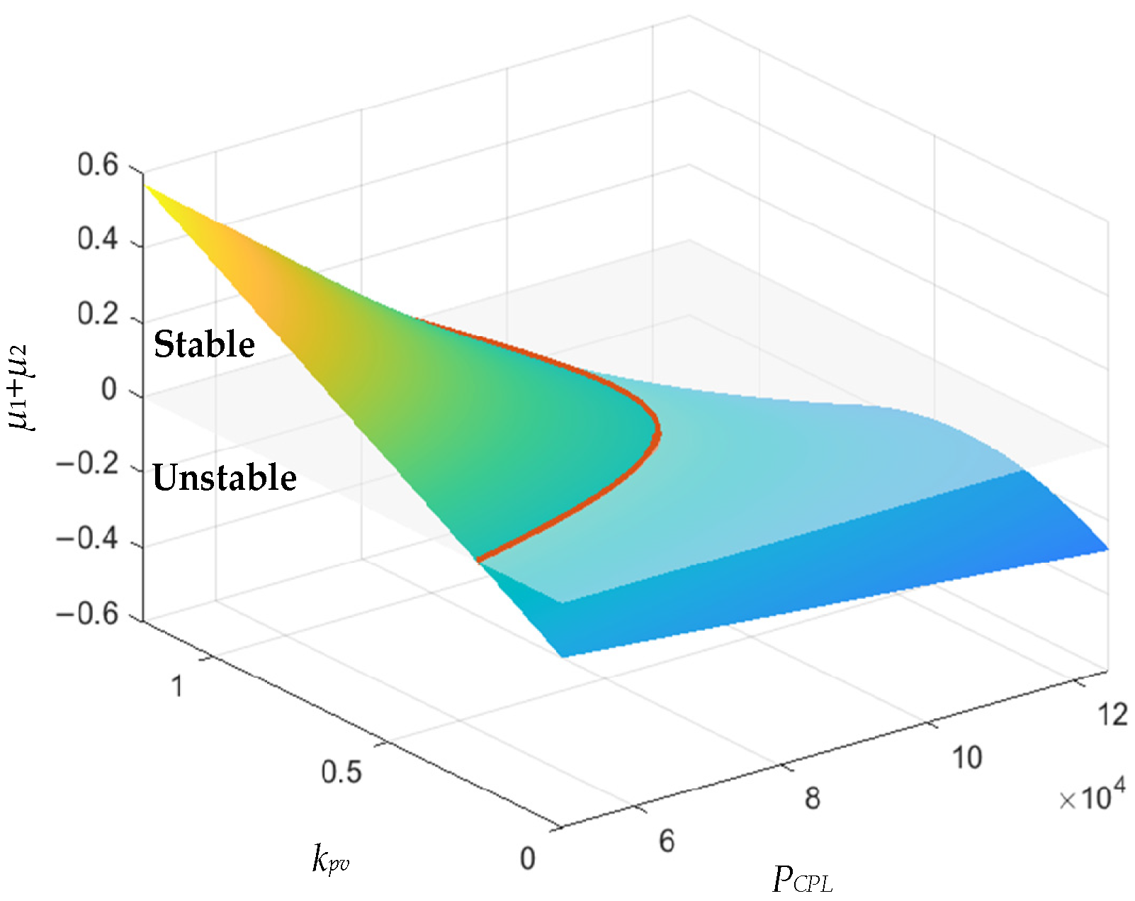
The system parameters are listed in Table 1. Let PCPL1 and PCPL2 denote two different constant power loads. The transient stability problem associated with a load step from PCPL1 to PCPL2 is then analyzed. When evaluating (38), the post-disturbance equilibrium point should be used as the integration reference. To assess system stability after the load step, PCPL in criterion (38) is set to PCPL2. According to the continuity of state variables, i.e., the switching theorem of capacitor voltage, inductor current and other state variables at the pre-disturbance equilibrium point are substituted into the calculation. By substituting the parameters in Table 1 into (37), the relationship among the stability index μ1 + μ2, the constant power load PCPL, and the proportional gain kpv of the outer voltage loop can be obtained, as shown in Figure 4.
In Figure 4, the intersection curve between the surface and the plane μ = 0 represents the large-signal stability boundary of the system. As can be seen, the effects of the constant power load PCPL and the proportional gain kpv on system stability are not linearly related. The stable operating region first expands and then contracts as kpv increases.
Reference [29] presents a stability criterion for the flexible interconnection system. By setting the DC voltage derivative dudc/dt = 0 and following the derivation procedure described above, the conventional stability criterion of the flexible interconnection system can be obtained as
P C P L < 3 u d c 2 u s d k p v + 2 3 i o 2 R f i d k p v L f i d k i v
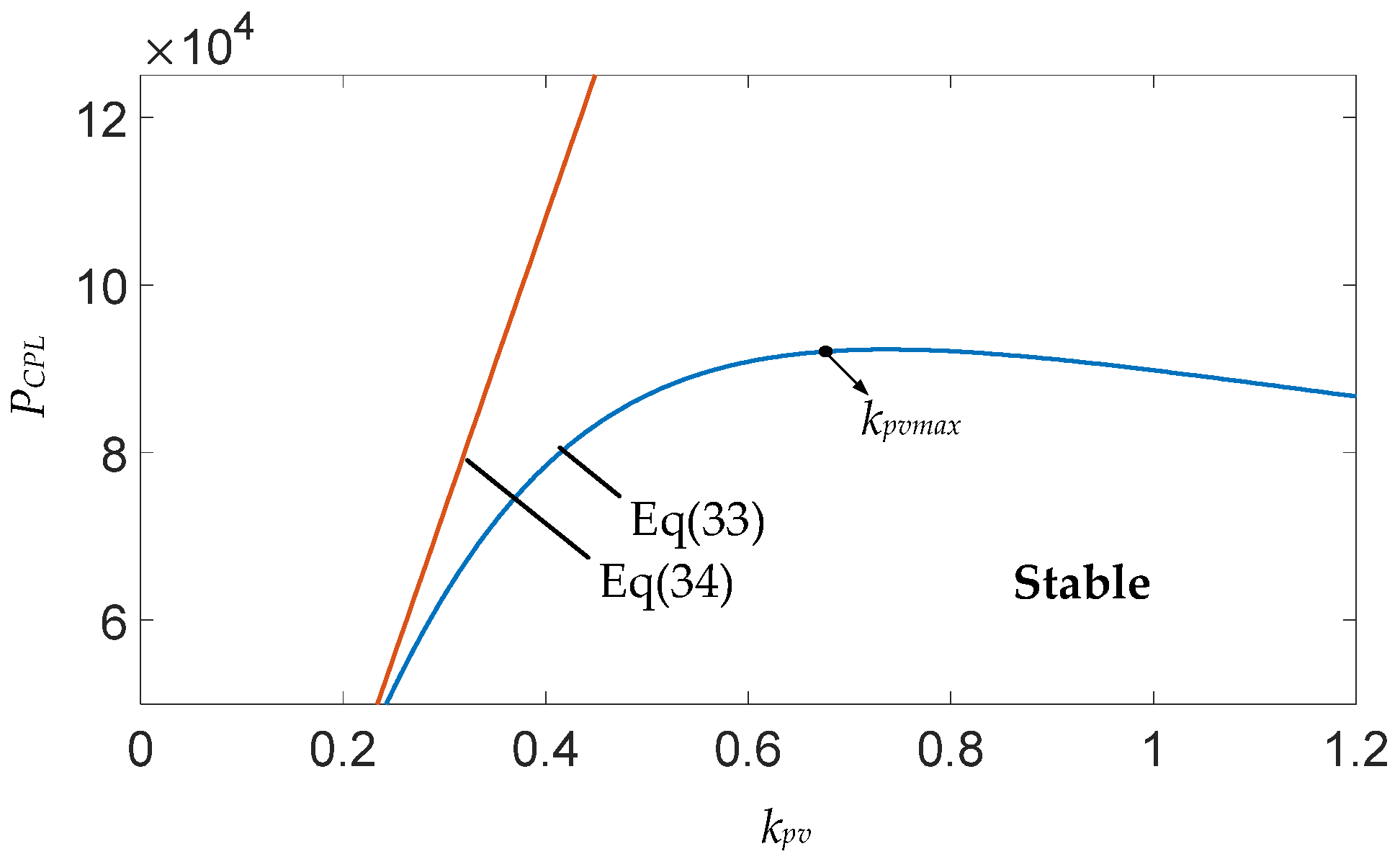
According to (39), the proportional gain kpv in the conventional criterion exhibits a linear relationship with the maximum load power PCPL that the system can support. To compare the differences between criterion (38) and criterion (39) more intuitively, the influence of kpv on system stability under the two criteria is shown in Figure 5. Here, kpvmax denotes the extremum point of the curve corresponding to (38).
Figure 5 shows that, with the other parameters fixed, the value of μ1 + μ2 in the criterion (39) is positively correlated with kpv; that is, a larger kpv implies a higher maximum stable load power and stronger stability. By contrast, for the proposed criterion (38), when kpv < kpvmax, system stability improves as kpv increases, whereas when kpv > kpvmax, system stability deteriorates as kpv continues to increase.
Under large disturbances, greater changes in the operating condition lead to more pronounced fluctuations in the DC voltage udc during the transient process. Since criterion (39) neglects the derivative of the DC bus voltage, a significant discrepancy arises between (38) and (39) when PCPL is large. As shown by the stable operating regions in Figure 5, a larger load power step causes larger fluctuations in udc and capacitor current iC; therefore, leading to a more pronounced difference between the two criteria.
According to the relationship between kpv and system stability shown in Figure 5, with the other parameters held constant, there exists an optimal value kpvmax that maximizes the loadable power of the system. Based on stability criterion (38), kpvmax satisfies
k p v max = L f i d k i v + L f ` i d k i v 2 + 2 C u s d 2 R f i d L f k i v u d c r e f u d c 2 3 L f u s d 2 R f i d L f k i v u d c r e f u d c
According to the criterion equation, when the denominator 1-A < 0, μ1 + μ2 cannot remain positive during the transition of the AC current id from id1 to id2 after the disturbance. Only when 1-A > 0 can the validity of the criterion be guaranteed throughout the entire transient process. Therefore, to ensure system stability, kpv must satisfy
k p v < 2 C d c u d c 3 L f i d
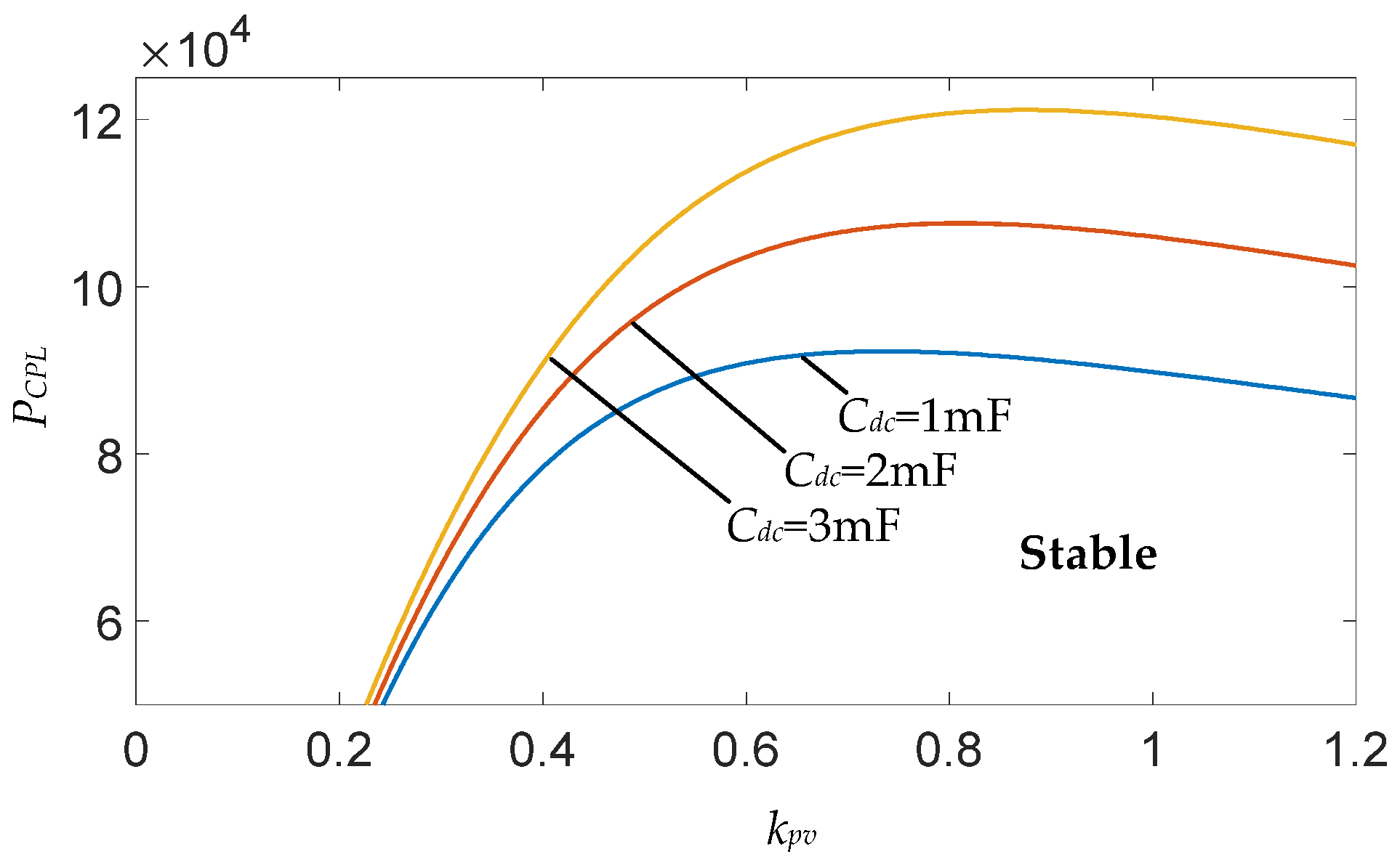
Based on criterion (38), and by substituting the parameters in Table 1, the stable operating ranges of the system under different DC capacitance values Cdc are shown in Figure 6.
Figure 6 shows that system stability is positively correlated with DC capacitance Cdc. Under the same set of other parameters, the stable operating region expands as Cdc increases. Comparing the relationship between kpv and stability for different capacitance values, a larger capacitance causes the stable operating boundary to approach the curve predicted by (39) in Figure 5 more closely. This indicates that only when the DC capacitance Cdc is sufficiently large does kpv exhibit an approximately linear relationship with the maximum permissible load PCPL. Under such a condition, criterion (38) becomes approximately equivalent to criterion (39).
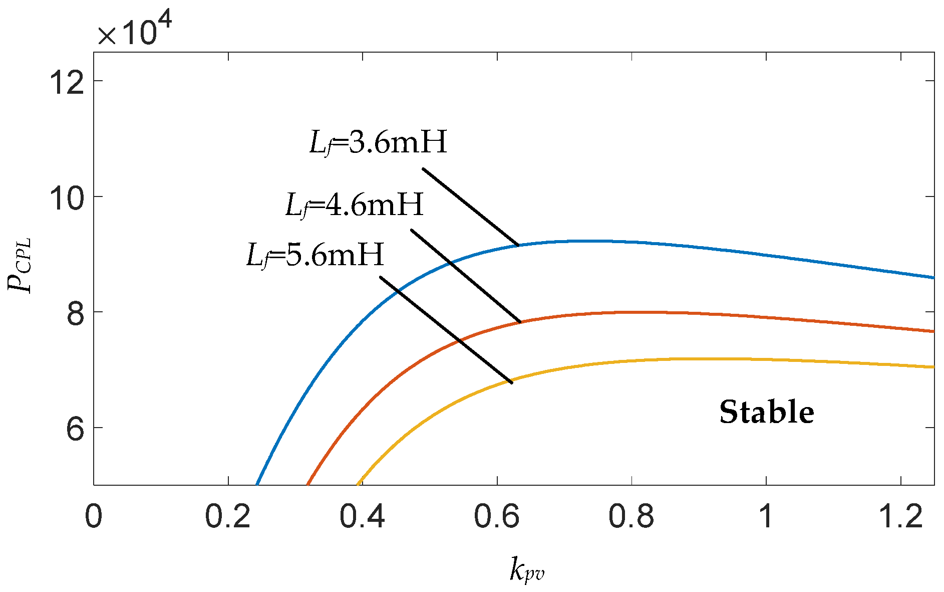
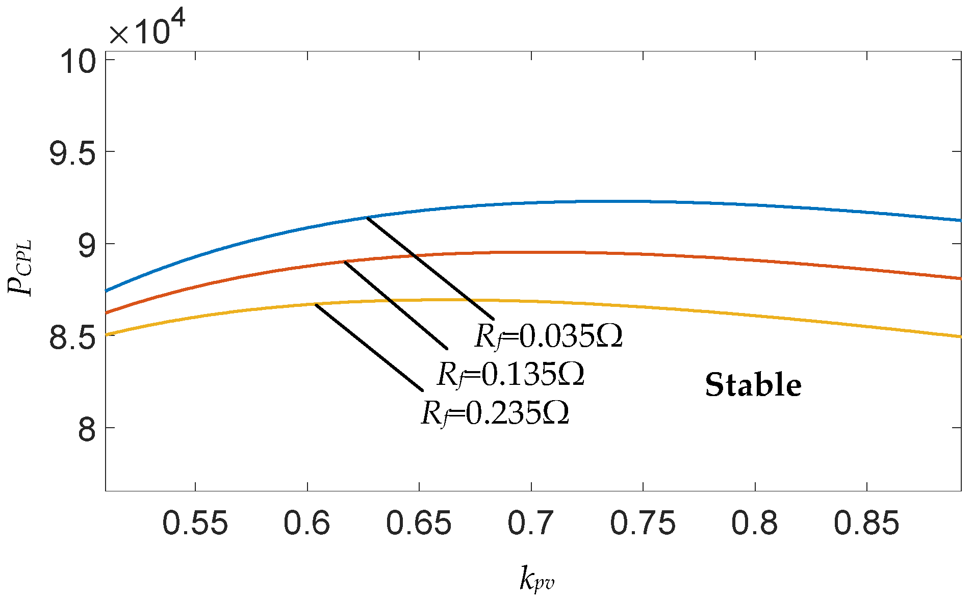
To further examine the influence of key parameters on the large-signal stability boundary, a sensitivity analysis is carried out by substituting the system parameters into criterion (38). Figure 7 illustrates the stable operating boundaries of the system under different equivalent resistance values Rf.
As illustrated in Figure 7, as the equivalent series resistance $R$ increases from 0.035 Ω to 0.235 Ω, the maximum allowable CPL step range decreases, indicating a deterioration in large-signal stability. From a physical viewpoint, a larger series resistance causes a more severe transient voltage drop across the line and filters elements during load surges. Owing to the constant-power characteristic of the CPL, the reduced DC bus voltage forces the load to draw a larger transient current to maintain power balance. This positive feedback effect aggravates the negative-impedance characteristic of the CPL and consequently reduces the large-signal stability region of the system. In addition, Figure 7 shows that the overall influence of Rf on system stability is relatively limited. For example, at kpv = 0.7, PCPL decreases only from 92 kW to 87 kW. Therefore, although practical parasitic losses in power electronic devices are unavoidable, the inherent conservativeness of MPF theory provides a sufficient stability margin to justify neglecting these minor losses in the theoretical model.
Similarly, based on criterion (38), Figure 8 shows the influence of different AC-side equivalent inductance values Lf on the stable operating range of the system.
As illustrated in Figure 8, the stable operating boundary of the system shrinks significantly as the AC-side equivalent inductance Lf increases. From a physical perspective, a larger front-end line inductance severely limits the slew rate (di/dt) of the grid-side current. When the system is subjected to a severe CPL step disturbance, excessive line inductance prevents the front-end rectifier from drawing energy from the AC grid in time to support the DC bus voltage. In particular, under weak grid conditions with a short-circuit ratio (SCR) below 3, where the grid-side impedance is very large, the large-signal stability of the system faces the most severe challenge.

4. Converter Stability Control Strategy Based on Power Differentiation Feedforward

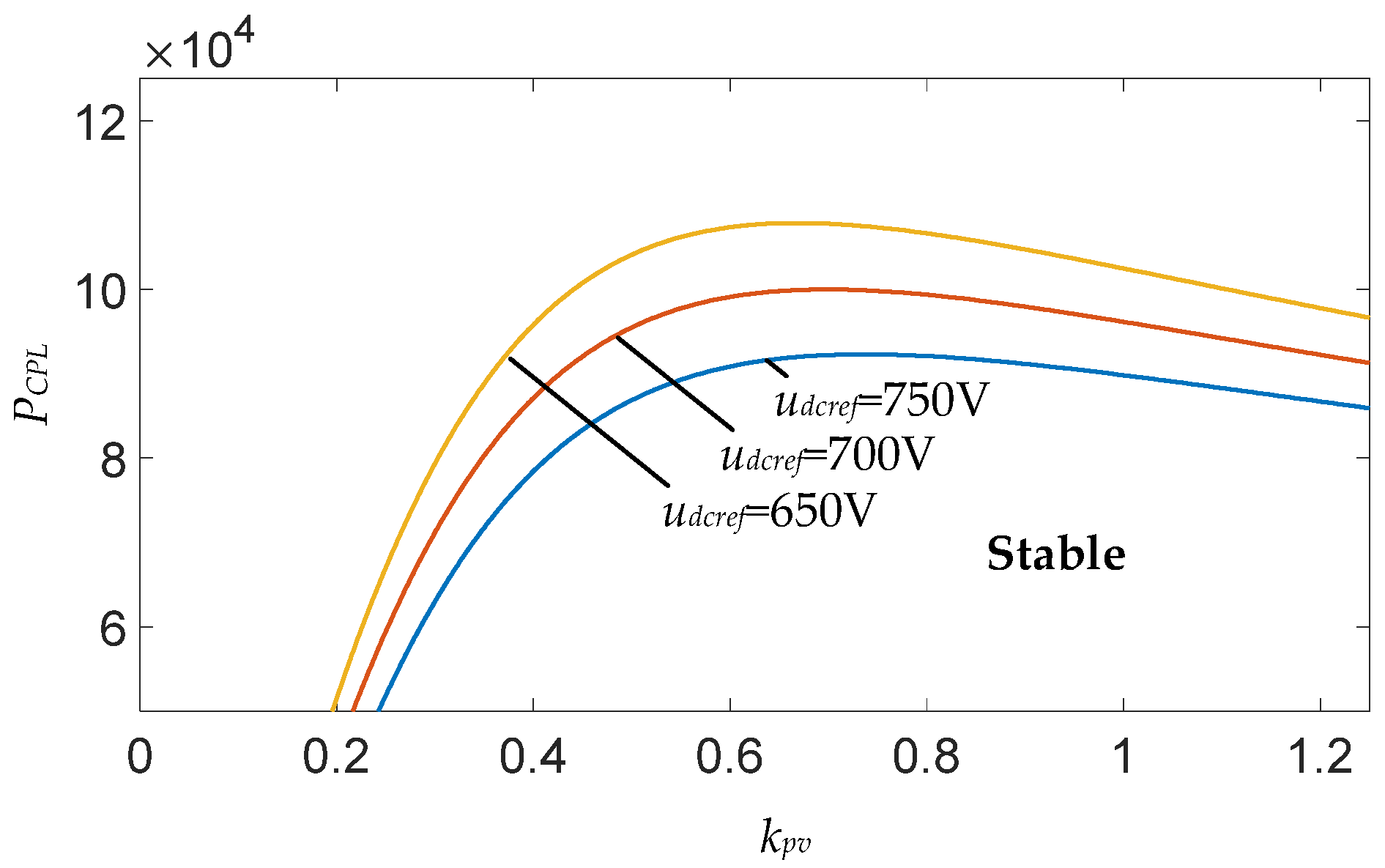
According to the stability criterion in (38), system stability is correlated with the DC voltage reference udcref. The stable operating range of the system under different values of udcref is shown in Figure 9.
As shown in Figure 9, with all other parameters held constant, a smaller DC voltage reference udcref corresponds to a larger maximum load power and stronger system stability. This indicates that moderately reducing udcref after a disturbance can effectively improve the large-signal stability of the system.
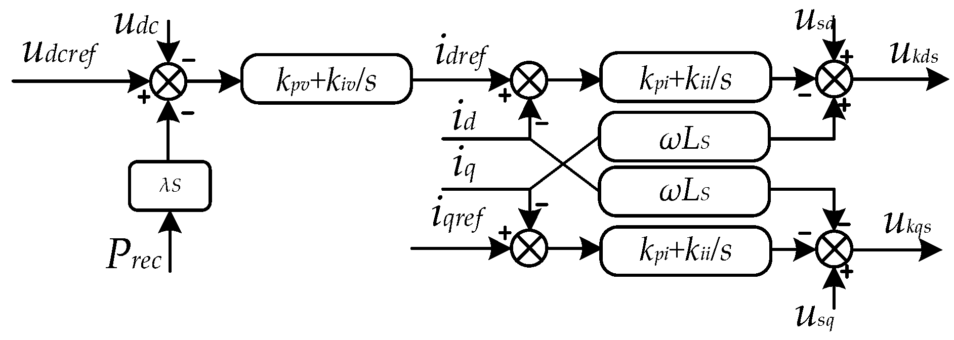
Although directly modifying the DC voltage reference udcref can improve system stability, load variations are often difficult to predict, making it challenging to adjust udcref in a timely manner after a disturbance. In addition, permanently changing the reference value may shift the operating point of the DC voltage away from its nominal range and potentially trigger undesired operating conditions or even faults. Therefore, this paper proposes a power differentiation feedforward control strategy that adjusts the voltage reference according to power variations. The corresponding control block diagram is shown in Figure 10.
As shown in Figure 10, the corresponding control law can be written as
i d r e f = k p v u d c r e f u d c λ d P r e c d t + k i v u d c r e f u d c λ d P r e c d t d t
where λ is the control coefficient to be designed. According to (42), the DC bus voltage is related to the rate of change in the rectifier power. When a load power step occurs, the rectifier output power changes rapidly toward a new operating point during the initial stage of the disturbance, resulting in a large derivative term. Consequently, the equivalent DC voltage reference decreases. During the later stage of the transient, as the system gradually approaches steady state and Prec becomes constant, the DC voltage udc returns to and remains at its nominal value. Compared with directly modifying the DC voltage reference, the proposed strategy introduces power feedforward to achieve adaptive voltage regulation while preventing the DC voltage from permanently deviating from its nominal operating point.
Next, the influence of the proposed strategy on system stability is analyzed on the basis of mixed potential function (MPF) theory.
For the flexible interconnection system shown in Figure 1, when the power differentiation feedforward control strategy is adopted, the expressions for the voltage potential function B(udc) and the DC current io still satisfy (14) and (19), respectively. Therefore, in the derivation of the stability criterion, it is only necessary to calculate the three partial derivatives in (21) and substitute them back into the criterion. Differentiating (42) with respect to time t and voltage udc, respectively, yields
d i d d t = k p v + λ k i v i o C d c P C P L u d c i o u d c + λ k i v P C P L λ k i v u d c i o C d c i o u d c d i d d t u d c = k p v + λ k i v i o C d c P C P L u d c 2 + i o u d c k i v + λ k i v C d c P C P L u d c i o i o u d c i d u d c = k p v λ k i v i o
Following a derivation similar to that in Section 3.3, substituting (43) into (21) yields the partial derivative of the DC current with respect to voltage:
i o u d c = 3 2 u d c u s d 2 R f i d k p v + λ k i v i o + 3 L f 2 u d c k p v + λ k i v i o P C P L u d c i o C d c u d c + λ k i v P C P L λ k i v u d c i o C d c i o u d c k p v + λ k i v i o 3 2 u d c L f i d k p v + λ k i v i o C d c P C P L u d c 2 + i o u d c k i v + λ k i v C d c P C P L u d c i o i o u d c i o u d c
Collecting like terms and isolating the current partial derivative term on the left-hand side yield
1 + 3 λ L f k i v 2 C d c u d c 2 P C P L u d c i o i d k p v + λ k i v i o u d c i o u d c = 3 2 u d c u s d 2 R f i d k p v + λ k i v i o + 3 L f i d k i v 2 u d c i o u d c + 3 L f 2 u d c k p v + λ k i v i o 2 P C P L u d c i o C d c u d c 3 L f i d 2 u d c k p v + λ k i v i o C d c B v v ( u d c )
After simplification, the partial derivative of the current can be obtained as
i o u d c = 1 1 + α 3 2 u d c N 2 k p v + λ k i v i o 2 L f P C P L C d c u d c + M 2 B v v ( u d c )
where α, M2, and N2 are intermediate variables introduced to simplify the mathematical expression, and they are defined as follows:
α = 3 λ L f k i v 2 C d c u d c 2 P C P L u d c i o i d k p v + λ k i v i o u d c M 2 = 3 L f i d 2 C d c u d c k p v + λ k i v i o N 2 = k p v + λ k i v i o u s d 2 R f i d L f i d k i v + 2 i o 3 + k p v + λ k i v i o 2 L f i o C d c
Substituting (46) into (16), the second-order partial derivative of the voltage potential function is obtained as
B v v ( u d c ) = 1 1 + α 3 2 u d c N 2 k p v + λ k i v i o 2 L f P C P L C d c u d c + M 2 B v v ( u d c ) P C P L u d c 2
Collecting like terms yields
B v v ( u d c ) = 1 1 + α M 2 3 2 u d c N 2 1 + α + 3 k p v + λ k i v i o 2 L f 2 C d c P C P L u d c 2
Based on (49), the minimum eigenvalues μ1 and μ2 of L−1/2Aii(i)L−1/2 and C−1/2Bvv(v)C−1/2, respectively, can be calculated as follows:
μ 1 = R f L f μ 2 = 1 C d c 1 + α M 2 3 2 u d c N 2 1 + α + 3 k p v + λ k i v i o 2 L f 2 C d c P C P L u d c 2
Accordingly, μ1 + μ2 is given by
μ 1 + μ 2 = 1 C d c 1 + α M 2 3 2 u d c N 2 1 + α + 3 k p v + λ k i v i o 2 L f 2 C d c P C P L u d c 2 + R f L f > 0
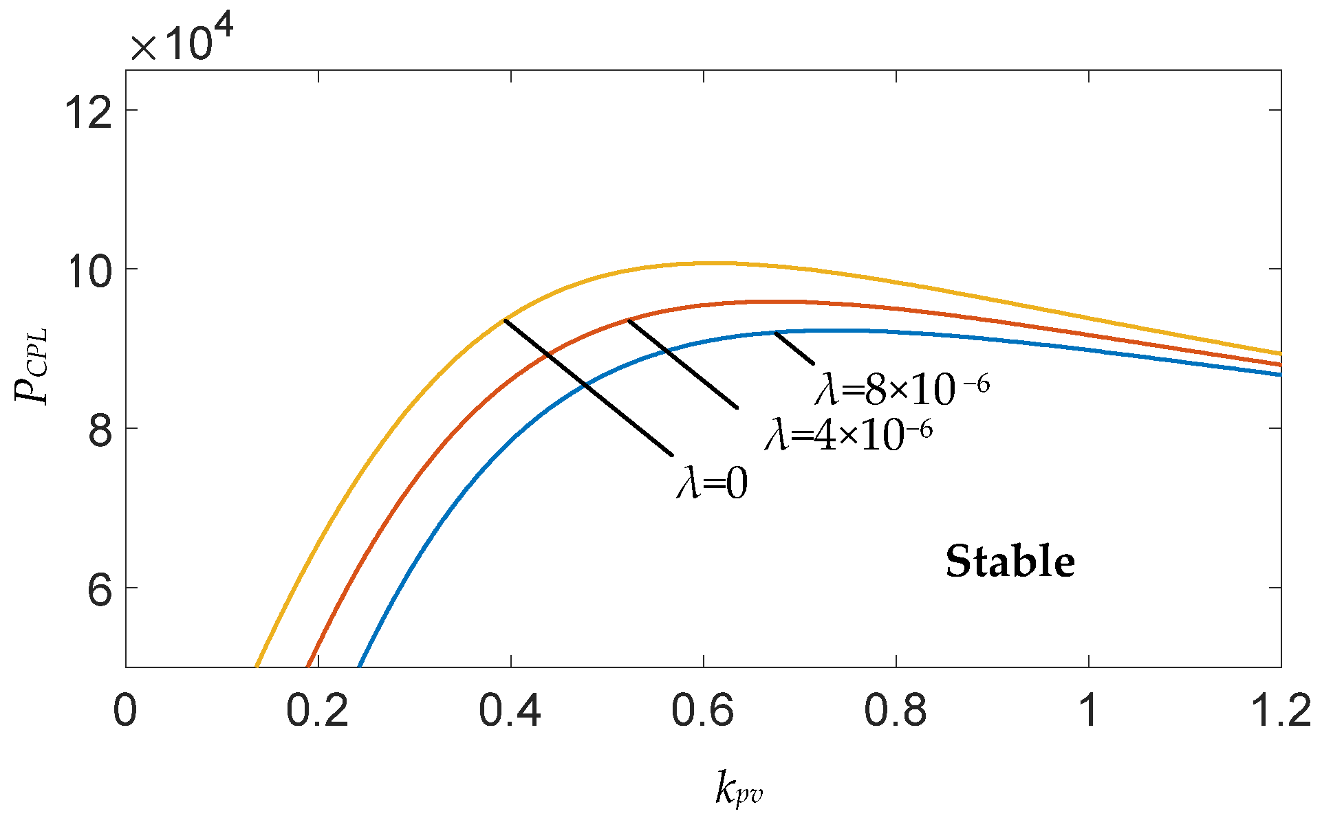
Compared with the stability criterion under constant DC voltage control, the criterion under the proposed strategy becomes more complex because of the additional power differentiation feedforward term. When λ = 0, the proposed power differentiation feedforward control degenerates into conventional constant DC voltage control. Under this condition, the derived criterion reduces to the original one. By substituting the parameters in Table 1 into the resulting criterion, the stable operating ranges under different control coefficients λ can be obtained, as shown in Figure 11.
As shown in Figure 11, compared with conventional constant DC voltage control (λ = 0), the stable operating range of the system expands after the introduction of power differentiation feedforward. With the other parameters unchanged, a larger λ, within a certain range, leads to stronger system stability. Meanwhile, increasing λ also enlarges the DC voltage dip following a disturbance. Similarly to the analysis in Section 3.4, to ensure system stability, the corresponding criterion must satisfy 1+α-M2 > 0, which implies that λ must satisfy
2 C d c u d c 2 + 3 λ L f k i v P C P L u d c i o i d k p v + λ k i v i o u d c 3 L f i d u d c k p v + λ k i v i o > 0
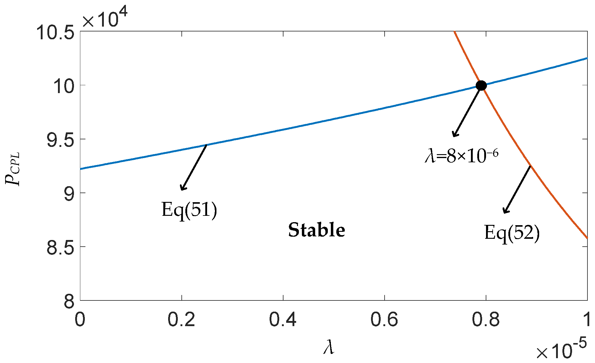
Clearly, (52) is a quadratic inequality with respect to λ. To identify the maximum stable operating range of the system, the stable operating regions under different values of λ are obtained by combining the corresponding stability criterion with (52) and substituting the relevant parameters from Table 1, as illustrated in Figure 12.
As shown in Figure 12, for the flexible interconnection system with the parameters listed in Table 1, the maximum stable operating range is achieved when λ = 8 × 10⁻⁶. Compared with conventional constant DC voltage control, the maximum allowable load step increases from 92 kW to 100 kW, corresponding to an improvement of 8.7%.
Beyond the theoretical expansion of the stability boundary, the practical engineering value of the proposed strategy also warrants attention. It should be noted that, although advanced nonlinear control methods such as model predictive control (MPC) and sliding mode control (SMC) can provide excellent dynamic performance during severe transients, their widespread industrial application remains constrained by several practical limitations. For example, MPC requires an accurate mathematical model and considerable real-time computational resources for rolling optimization, often necessitating high-performance and costly digital controllers.
By contrast, the feedforward control strategy proposed in this paper is highly attractive from an engineering perspective because of its simplicity. It improves the large-signal stability margin without abandoning the mature and widely adopted proportional–integral (PI) control framework. Moreover, the proposed method introduces only a negligible computational burden, making it a cost-effective and easily deployable solution for upgrading existing DC microgrid systems.

5. Simulation Verification

A two-terminal flexible interconnection system (FIS), as shown in Figure 1, is built in MATLAB/Simulink R2022b to verify the derived large-signal stability criterion and the proposed power differentiation feedforward control strategy. The system parameters are listed in Table 1. The rectifier adopts a dual-loop control structure consisting of an AC-side inner current loop and a DC-side outer voltage loop, whereas the inverter operates under PQ control to maintain constant output power. In the simulations, large disturbances are introduced through step changes in the active power reference of the inverter.

5.1. Verification of the Validity of the Proposed Criterion

Based on the system parameters listed in Table 1, substituting the corresponding values into the large-signal stability criterion (38) yields the maximum constant power load (CPL) that the system can withstand:
P C P L 92 kW
According to (53), with an initial power of 50 kW, the maximum allowable total CPL power is less than 92 kW. Table 2 lists two simulation cases with different load steps. Group I satisfies criterion (38), whereas Group II does not.
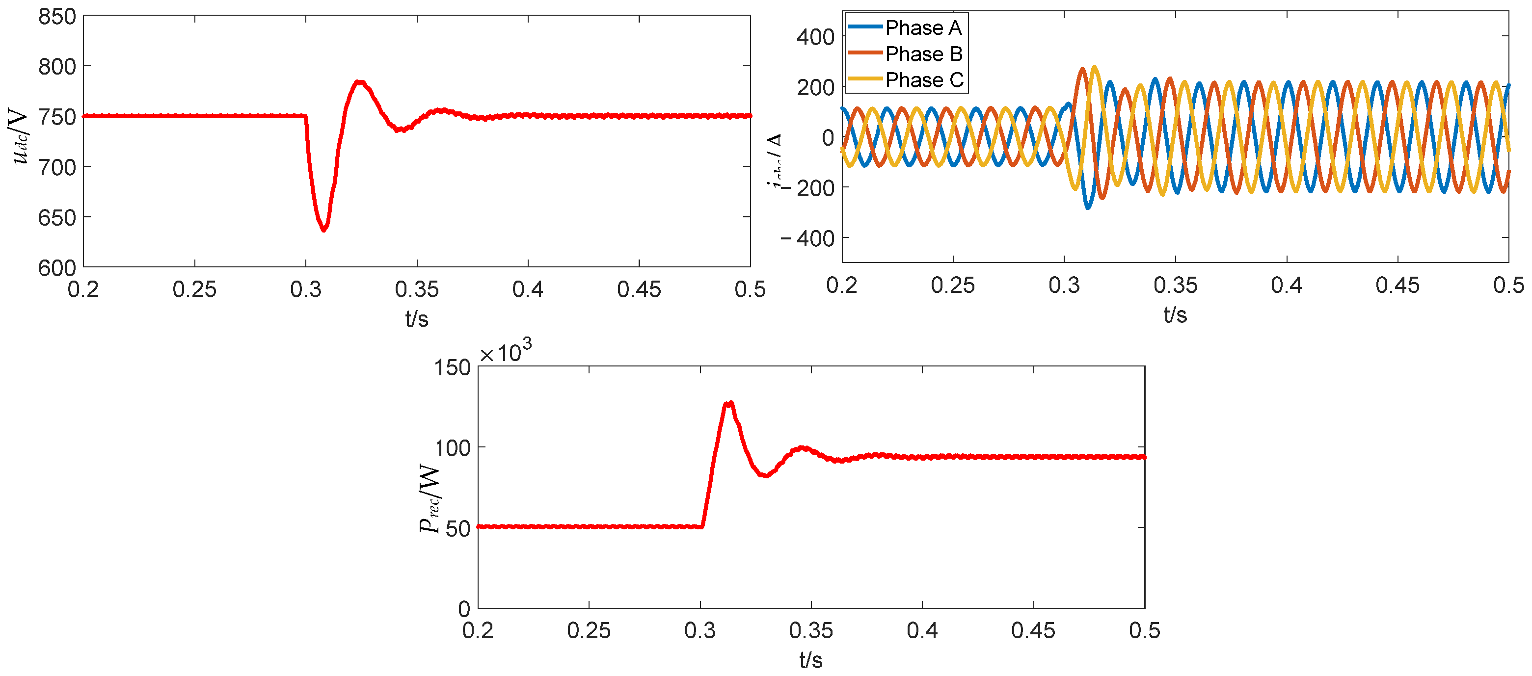
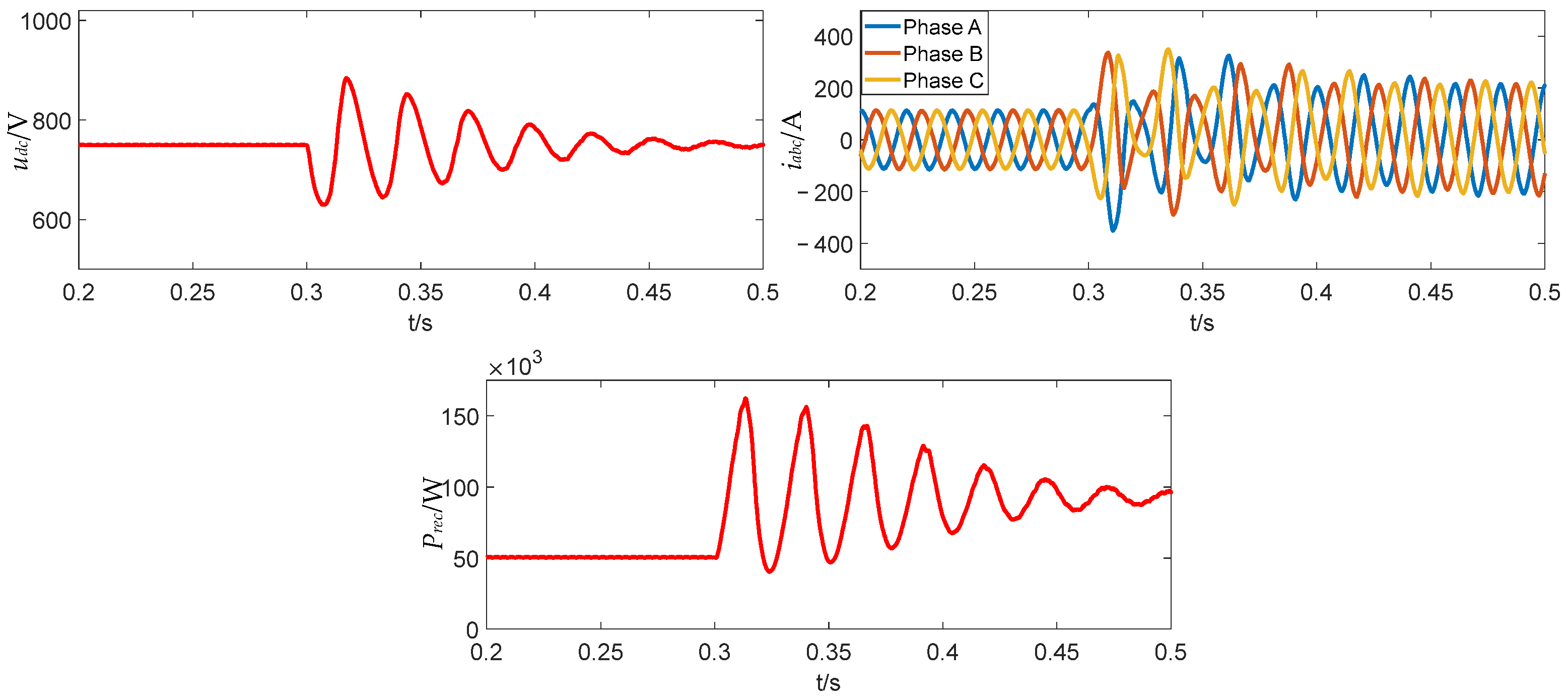
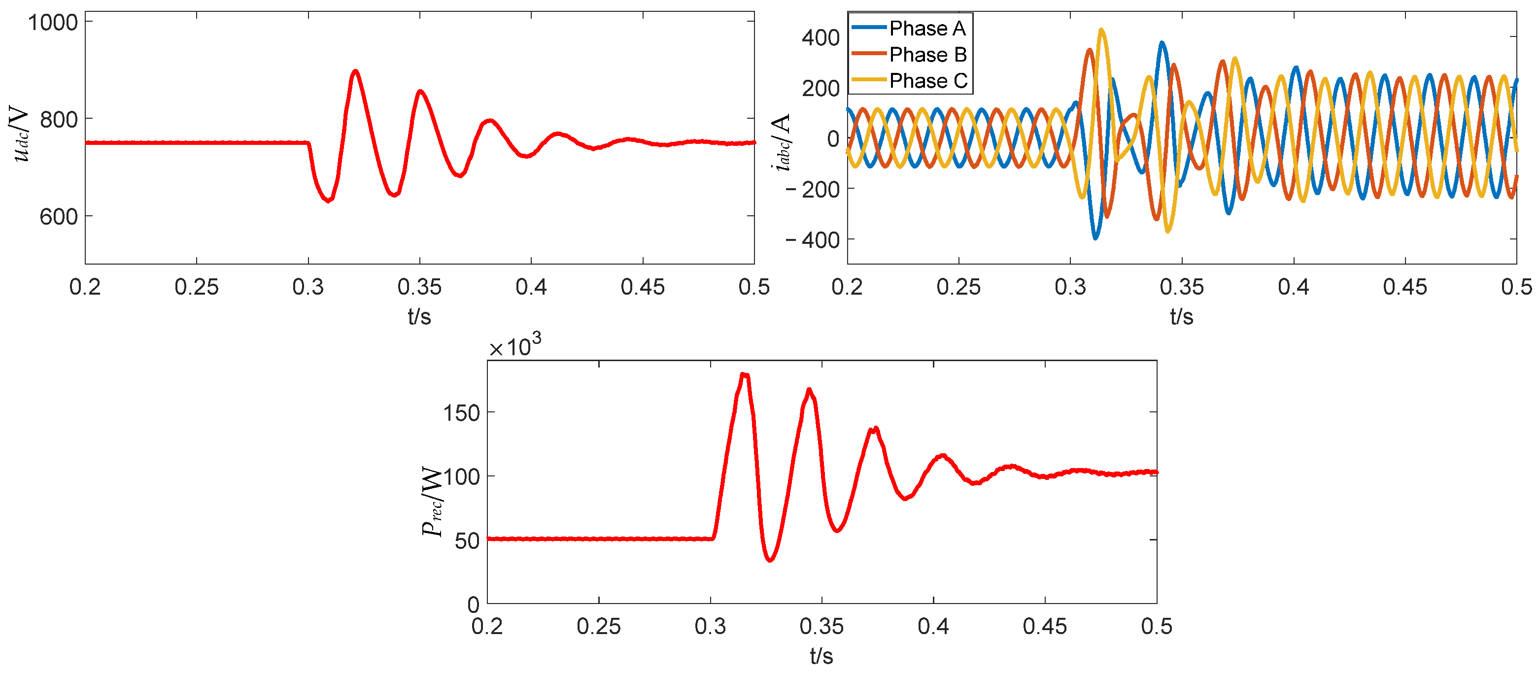
Case I: The inverter-side load power steps from 50 kW to 92 kW using the parameters of Group I. The simulation results are shown in Figure 13.
As shown in Figure 13, the CPL steps from 50 kW to 92 kW at t = 0.3 s. After an oscillatory transient lasting approximately 0.15 s, the DC bus voltage recovers to 750 V, and the AC-side three-phase currents gradually return to normal. This response indicates that, although the flexible interconnection system (FIS) remains stable, it is already operating close to the critical stability boundary. This simulation result is fully consistent with the theoretical prediction of criterion (38).
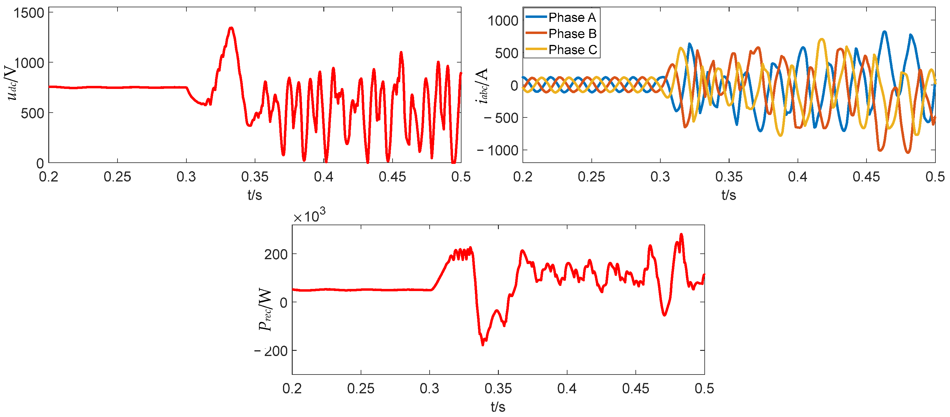
Case II: The inverter-side CPL power PCPL steps from 50 kW to 100 kW. The simulation results are shown in Figure 14.
As shown in Figure 14, when the load steps to 100 kW at t = 0.3 s, the h can no longer be maintained at 750 V, and the AC-side three-phase currents become unstable. This confirms that the flexible interconnection system cannot operate stably when the load step violates criterion (38).
In summary, the system becomes unstable when the power step exceeds the range predicted by the criterion. This verifies the accuracy of the large-signal stability criterion (38) derived in this paper.
Next, the influence of the proportional gain kpv and the DC capacitance Cdc on large-signal stability is further examined.
Figure 5 compares the proposed stability criterion (38) with the conventional criterion (39). With the other parameters held constant, criterion (39) suggests that the stable operating range increases linearly with kpv. However, according to the proposed criterion (38), stability becomes negatively correlated with kpv when kpv > 0.7.
When kpv = 1.2, criterion (38) indicates that the allowable inverter-side load power satisfies
P C P L 86 kW
According to (54), if kpv in Group I is increased from 0.7 to 1.2 while all other parameters remain unchanged, the maximum load power limit decreases from 92 kW to approximately 86 kW. Consequently, a load step to 92 kW exceeds the allowable limit, and the system should become unstable. Table 3 summarizes the simulation cases under different kpv values.
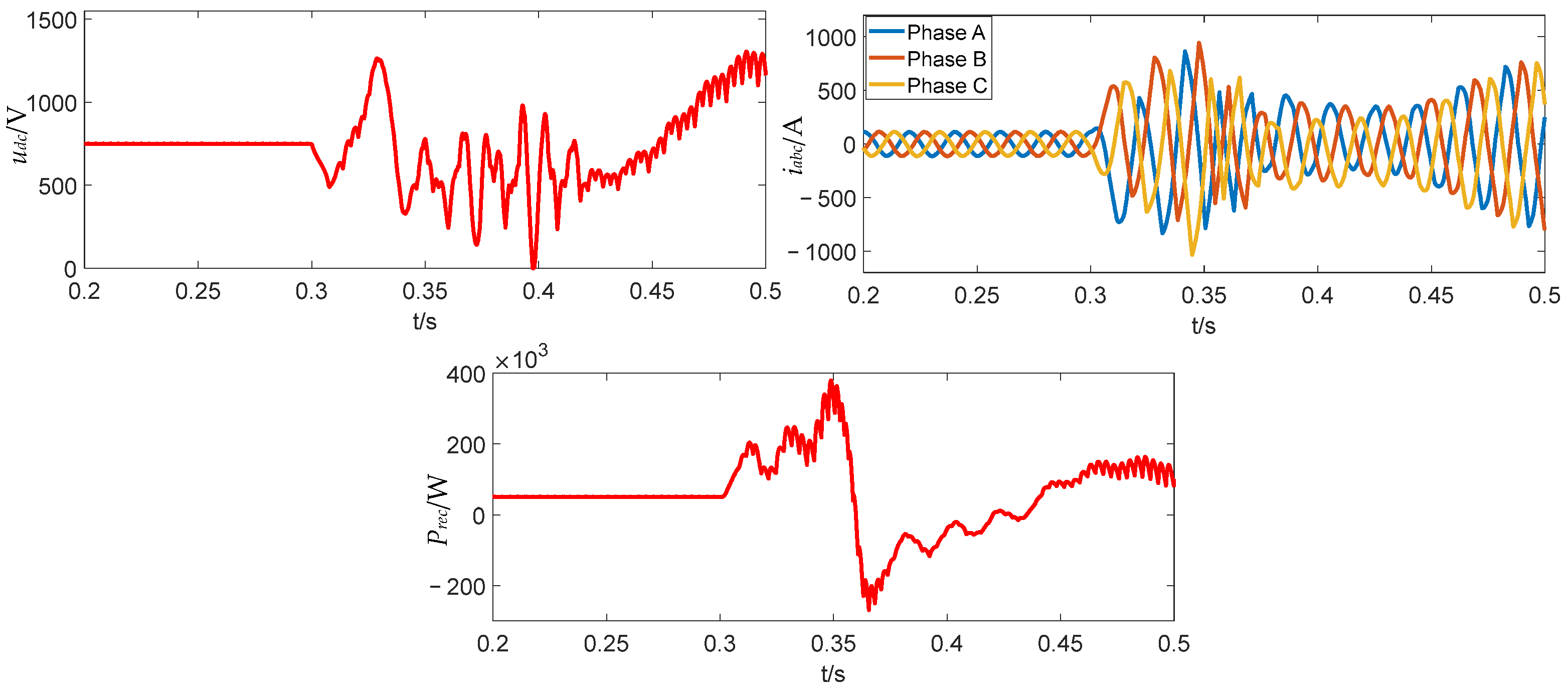
Case III: Under the condition kpv = 1.2, the load power PCPL steps from 50 kW to 92 kW. The simulation results are shown in Figure 15.
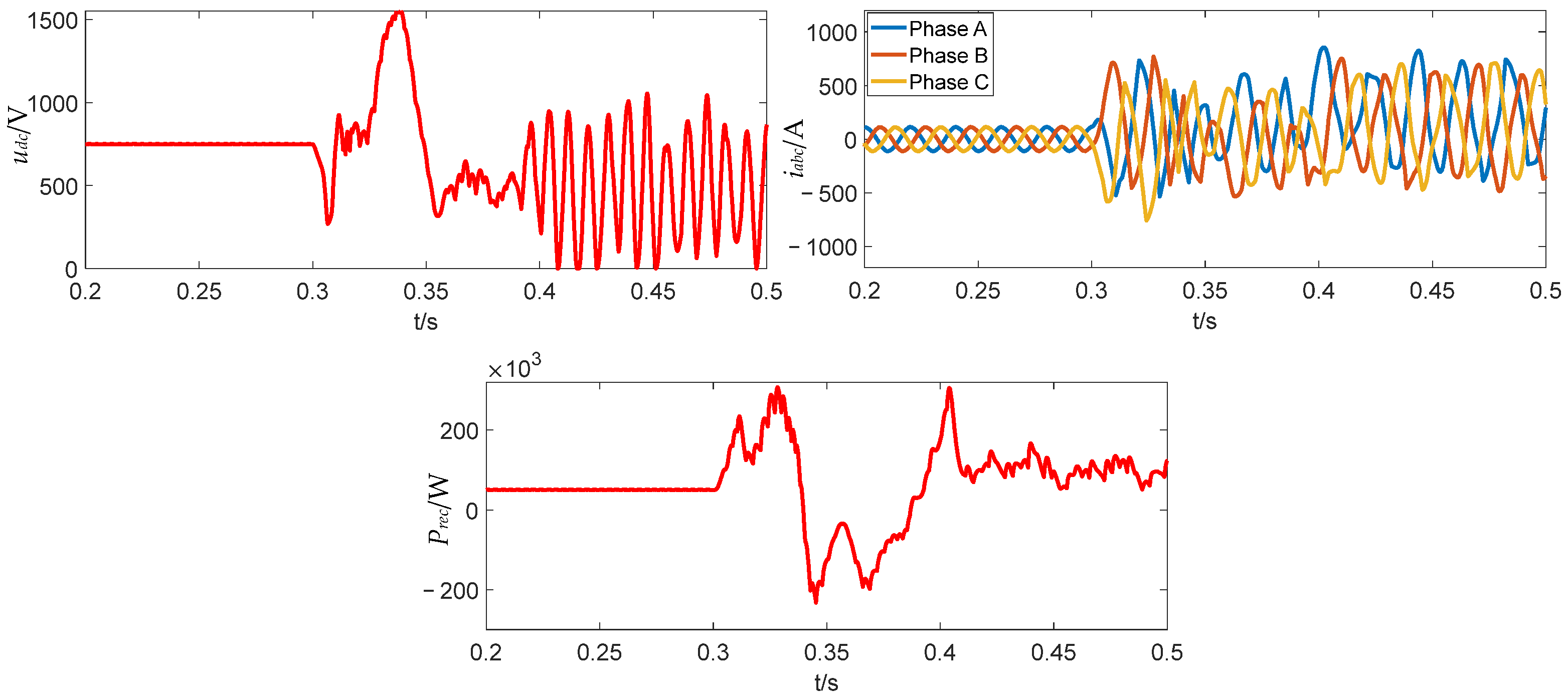
Case IV: Under the condition kpv = 0.4, the load power PCPL steps from 50 kW to 92 kW. The simulation results are shown in Figure 16.
Comparing Cases I, III, and IV under the same load step (50 kW→92 kW), Figure 13, Figure 15, and Figure 16 show that when kpv = 0.4 or kpv = 1.2, the DC bus voltage drops and oscillates after the disturbance and fails to recover to the rated value, while the AC-side currents become unstable. The system remains stable only when kpv = 0.7.
More importantly, Case III (kpv = 1.2) exhibits instability in the simulation. This result contradicts the prediction of the conventional criterion (39), which suggests improved stability, but agrees with the proposed criterion (38), which predicts a reduced stability margin (PCPL < 86 kW). This demonstrates that the proposed criterion (38) predicts the stable operating range under large disturbances more accurately than criterion (39).
Case V: With Cdc = 2 mF, the load power PCPL steps from 50 kW to 100 kW. The simulation results are shown in Figure 17.
According to criterion (38), increasing Cdc raises the maximum allowable power limit. When Cdc is increased to 2 mF, with all other parameters unchanged, the system is subjected to the same disturbance as in Case II (50 kW→100 kW). As shown in Figure 17, after the load step at t = 0.3 s, the DC bus voltage returns to 750 V, and the AC-side currents remain stable. This behavior differs from that in Case II (Cdc = 1 mF), confirming that increasing the DC capacitance improves system stability, which is consistent with the analysis in Figure 6.

5.2. Verification of the Proposed Control Strategy

In practical industrial applications, the dynamic reconstruction of the DC voltage induced by the power differentiation feedforward term must be coordinated with the over-voltage and under-voltage protection thresholds of the converter hardware. To prevent the reconstructed voltage reference from triggering under-voltage lockout during transients, an additional saturation limit is imposed on the DC voltage reference command. In this paper, the reference variation is constrained within a safe operating range of 650 V to 800 V throughout the transient process.
According to the stability criterion derived for the proposed feedforward strategy, adding power differentiation feedforward to the dual-loop control system increases the allowable power step limit and enables the system to remain stable under conditions that would otherwise lead to instability. As shown in Figure 12, when the power differentiation feedforward control is adopted with λ = 8 × 10⁻⁶, the maximum load step satisfies
P C P L 100 kW
According to (55), if the system in Group II, which previously became unstable, adopts the proposed control strategy, it should remain stable. To verify this, the rectifier control is modified according to Figure 10, with λ = 8 × 10⁻⁶ and all other parameters unchanged from Table 1. The specific load-step settings in the two new simulation cases are summarized in Table 4.

5.2.1. Verification Under Severe CPL Surges

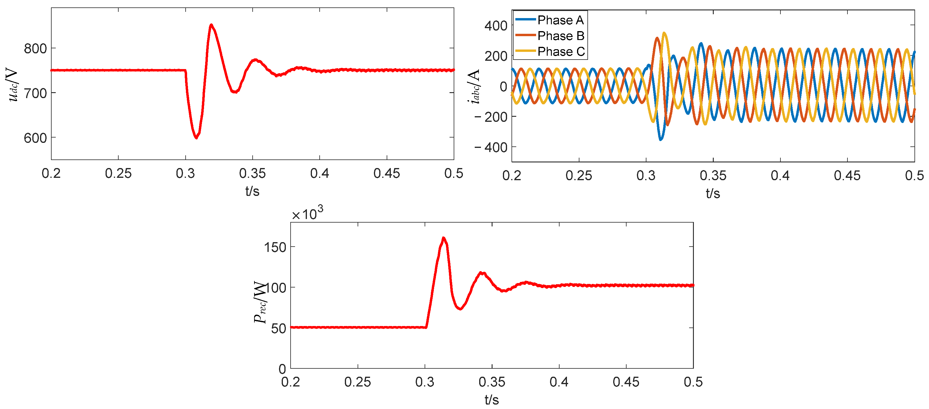
Case VI: Under power differentiation feedforward control, the load power PCPL steps from 50 kW to 92 kW. The simulation results are shown in Figure 18.
As shown in Figure 18, the system remains stable under the proposed feedforward control. Compared with Figure 13, the voltage nadir is improved from 627 V to 638 V. When a load surge occurs (dPrec/dt > 0), the feedforward term proactively reduces the voltage reference udcref to track the inevitable transient decline in the actual DC voltage udc. This dynamic tracking limits the PI controller input error eu = udcrefudc, thereby suppressing integral windup and preventing excessively aggressive instantaneous current commands. Consequently, the system draws energy from the grid at a smooth and controlled did/dt rate. As the disturbance decays, udcref gradually returns to 750 V without overshoot. By providing a transient buffering effect, the proposed strategy effectively suppresses DC voltage fluctuations and expands the large-signal stability boundary.
Case VII: Under power differentiation feedforward control, the load power PCPL steps from 50kW to 100kW. The simulation results are shown in Figure 19.
Figure 19 shows the simulation results under the proposed control. At t = 0.3 s, the load steps from 50 kW to 100 kW. Under the action of the feedforward control, the DC bus voltage stabilizes at 750 V after the disturbance, and the AC-side currents remain stable. Compared with the corresponding case without feedforward control, the proposed strategy exhibits enhanced disturbance rejection capability and maintains stable operation. These simulation results are consistent with the theoretical analysis of Figure 11 and verify the effectiveness of the proposed stability control strategy.

5.2.2. Performance Under Weak Grid Conditions

To further evaluate the robustness of the proposed control strategy under severe grid conditions, the simulation scenario is extended to a weak grid environment. In practical flexible interconnection systems, a weak AC grid usually exhibits a low short-circuit ratio (SCR) and a large equivalent grid impedance, which significantly reduces system damping and challenges large-signal stability during transients.
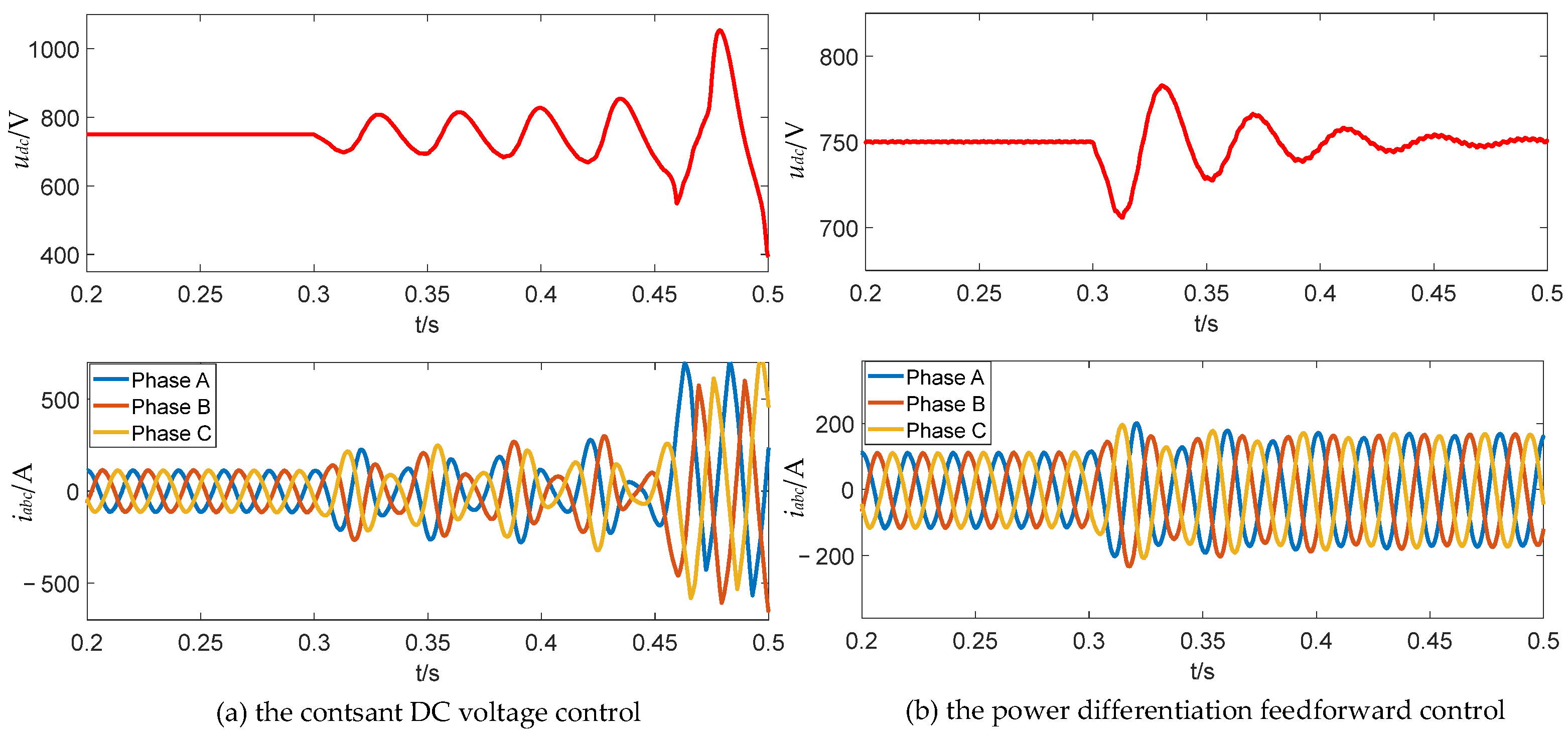
In Case VIII, an extremely weak grid condition with an SCR of 1.5 is considered. Based on the rated power and rated voltage of the system, the grid-side line impedance parameters are calculated as Rr = 0.2 Ω and Lr = 3 mH, assuming an X/R ratio of 5. At t = 0.3 s, a large-signal disturbance is applied, in which the constant power load steps from 50 kW to 65 kW.
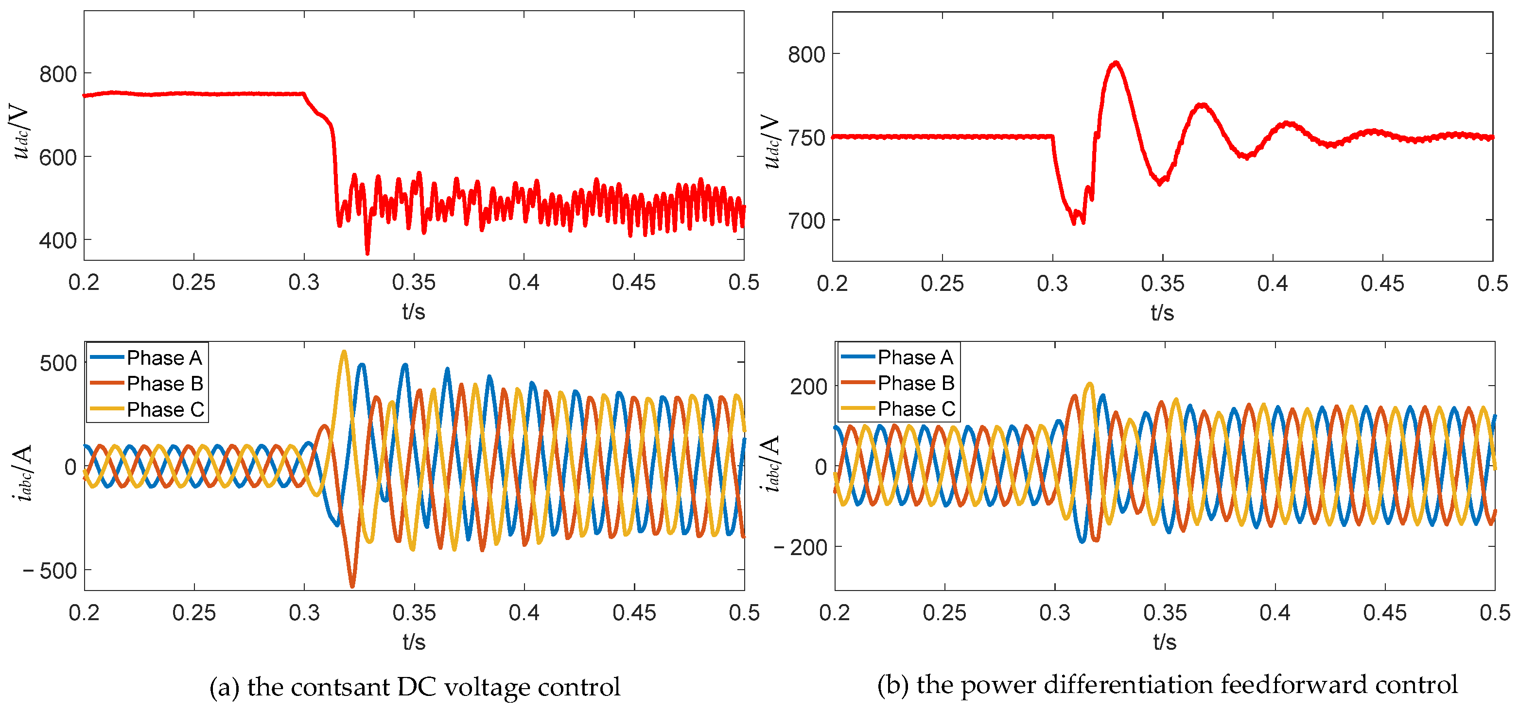
Figure 20 compares the dynamic responses under the two control strategies. As shown in Figure 20a, under conventional PI control, the severe weak grid condition leads to rapid voltage collapse. After the disturbance, the DC bus voltage drops to approximately 400 V, indicating a complete loss of large-signal stability. By contrast, the proposed feedforward control shown in Figure 20b successfully maintains system stability. Despite the very high grid impedance, the DC voltage dip is effectively limited to about 700 V before rapidly recovering to the nominal value of 750 V, and the AC-side currents transition smoothly to the new steady state. This result clearly demonstrates the robustness of the proposed strategy in preventing voltage collapse under severe weak grid conditions.

5.2.3. Robustness Against AC Voltage Sags

Although the stability criterion in (38) is derived specifically for severe nonlinear instability caused by CPLs, practical DC microgrids are also subject to external AC-grid disturbances. To further verify the overall robustness of the proposed control strategy, an additional simulation is conducted under a symmetrical AC-grid voltage sag.
Figure 21 compares the dynamic responses of the system under the two control strategies during a 31% AC voltage sag. As shown in Figure 21a, under conventional PI control, the transient power delivery interruption caused by the grid fault induces severe and divergent oscillations in the DC bus voltage, ultimately leading to instability. By contrast, as illustrated in Figure 21b, the proposed feedforward control exhibits strong disturbance rejection capability. It rapidly mitigates the transient power mismatch, effectively suppresses DC voltage fluctuations, and maintains the DC voltage around its nominal value of 750 V, while the AC-side currents smoothly return to steady state. This further confirms that the proposed strategy not only handles large-signal load step disturbances effectively but also maintains satisfactory stability performance under severe grid-side voltage sags.

6. Discussion

In practical distributed DC microgrids and flexible interconnection systems (FISs), advanced droop control techniques have been extensively studied. For example, dynamic decentralized droop control has been proposed to facilitate high-efficiency renewable energy integration in microgrid systems [30]. Although such decentralized strategies can effectively achieve steady-state power sharing, they inherently introduce steady-state voltage deviations, which may continuously reduce the large-signal stability margin in systems containing constant power loads (CPLs). By contrast, the power differentiation feedforward strategy proposed in this paper acts strictly as a transient compensator. Since it only modifies the local voltage reference on the basis of local measurements, it is inherently a decentralized control method. Therefore, it can be naturally integrated into individual source nodes in complex multi-terminal systems. In this way, critical local nodes can be reinforced against severe transient CPL surges while the global power-sharing capability of the network and the efficient integration of renewable energy are preserved.
Although the proposed control strategy is physically scalable and easy to implement, the analytical scope of this study should also be clearly stated. The rigorous large-signal stability criterion and the corresponding parameter optimization results presented in this paper are mathematically derived from a simplified two-terminal source-load model. This fundamental framework provides useful physical insight and guarantees the local stability of individual converter nodes. However, it may not fully capture the dynamic complexity of modern multi-terminal or mesh-connected FISs. In such networked systems, dynamic interactions, power flow redistribution, and cross-coupling through line impedances become increasingly important. Therefore, extending the current mixed potential function (MPF) methodology to construct a global energy function for mesh networks, and thereby enabling network-level large-signal stability assessment, remains an important and challenging direction for future research.

7. Conclusions

Focusing on a typical two-terminal flexible interconnection system, this paper establishes a system model based on the mixed potential function (MPF) method. By incorporating the dynamic characteristics of the DC-side capacitor, a novel large-signal stability criterion is derived. Furthermore, an improved control strategy for enhancing the disturbance rejection capability of the system is proposed and verified through MATLAB/Simulink simulations. The main conclusions are summarized as follows:
1. The proposed stability criterion reveals the constraint relationships among key circuit and control parameters, including the constant power load (CPL), the PI parameters of the rectifier voltage loop, and the DC-side shunt capacitance. Unlike conventional large-signal stability analyses, the proposed criterion explicitly accounts for the effect of the DC voltage derivative, or equivalently the capacitor current, on system stability. In addition, it enables PI parameter optimization under stability constraints, thereby providing useful theoretical guidance for controller design.
2. The proposed power differentiation feedforward control strategy dynamically reshapes the DC voltage reference during transient events, thereby suppressing voltage fluctuations and improving the disturbance rejection capability of the system. By actively mitigating transient power mismatch, the strategy enhances large-signal stability without relying heavily on additional hardware buffering devices. As a result, the method shows strong practical potential for maintaining continuous operation under severe CPL power steps and grid-side voltage sags.
Future work will focus on integrating the proposed strategy with advanced nonlinear control methods, such as model predictive control (MPC), and experimentally validating its practical robustness through hardware-in-the-loop (HIL) testing.

Author Contributions

Writing—original draft preparation: C.G.; writing—review and editing: H.Z.; supervision: X.Y. and W.X.; methodology and software: C.Z. and Z.L.; All authors have read and agreed to the published version of the manuscript.

Funding

This project is supported by the National Natural Science Foundation of China (52367019) and the Guizhou Province Science and Technology Support Plan (Qiankehe Support [2023] General 292).

Data Availability Statement

The original contributions presented in the study are included in the article; further inquiries can be directed to the corresponding author.

Conflicts of Interest

The authors declare no conflicts of interest.

References

  1. Xie, X.; Liu, Y.; Wang, X.; Han, Y. On Constructing New-Type Power Systems in China. CSEE J. Power Energy Syst. 2025, 11, 2710–2728. [Google Scholar] [CrossRef]
  2. Li, J.; He, Y.; Xu, L.; Liu, J. Design of Hybrid Power Filters for Supraharmonics Suppression in Power Electronics Dominated Power Systems. IEEE J. Emerg. Sel. Top. Power Electron. 2024, 12, 2163–2175. [Google Scholar] [CrossRef]
  3. Imdadullah; Amrr, S.M.; Jamil Asghar, M.S.; Ashraf, I.; Meraj, M. A Comprehensive Review of Power Flow Controllers in Interconnected Power System Networks. IEEE Access 2020, 8, 18036–18063. [Google Scholar] [CrossRef]
  4. Liu, H.; Deng, Z.; Li, X.; Guo, L.; Huang, D.; Fu, S.; Chen, X.; Wang, C. The Averaged-value Model of a Flexible Power Electronics Based Substation in Hybrid AC/DC Distribution Systems. CSEE J. Power Energy Syst. 2022, 8, 452–464. [Google Scholar] [CrossRef]
  5. Hosseinpour, H.; MansourLakouraj, M.; Benidris, M.; Livani, H. Large-Signal Stability Analysis of Inverter-Based AC Microgrids: A Critical and Analytical Review. IEEE Access 2023, 11, 111466–111491. [Google Scholar] [CrossRef]
  6. Song, Q.; Chen, J.; Loo, K.-H.; Chen, J.; Chen, P. Large-Signal Stability Analysis of Two-Stage Cascaded DC/DC Converter Systems Using Sum-of-Squares Programming. IEEE Trans. Power Electron. 2024, 39, 2076–2085. [Google Scholar] [CrossRef]
  7. Pal, D.; Panigrahi, B.K.; Johnson, B.; Venkatramanan, D.; Dhople, S. Large-Signal Stability Analysis of Three-Phase Grid-Following Inverters. IEEE Trans. Energy Convers. 2025, 40, 2696–2709. [Google Scholar] [CrossRef]
  8. Du, Y.; Men, Y.; Ding, L.; Lu, X. Large-Signal Stability Analysis for Inverter-Based Dynamic Microgrids Reconfiguration. IEEE Trans. Smart Grid 2023, 14, 836–852. [Google Scholar] [CrossRef]
  9. Liu, Z.; Ge, X.; Su, M.; Han, H.; Xiong, W.; Gui, Y. Complete Large-Signal Stability Analysis of DC Distribution Network via Brayton-Moser’s Mixed Potential Theory. IEEE Trans. Smart Grid 2023, 14, 866–877. [Google Scholar] [CrossRef]
  10. Fu, X.; Sun, J.; Huang, M.; Tian, Z.; Yan, H.; Iu, H.H.C.; Hu, P.; Zha, X. Large-Signal Stability of Grid-Forming and Grid-Following Controls in Voltage Source Converter: A Comparative Study. IEEE Trans. Power Electron. 2021, 36, 7832–7840. [Google Scholar] [CrossRef]
  11. Duan, Z.; Meng, Y.; Duan, Y.; Zhang, H.; Wang, X.; Wang, X. Large-Signal Stability Analysis and Enhancement of Modular Multilevel Matrix Converter Under Power Fluctuation Based on T-S Fuzzy Model Theory. IEEE Trans. Power Electron. 2023, 38, 14601–14613. [Google Scholar] [CrossRef]
  12. Wu, Z.; Han, H.; Liu, Z.; Su, M.; Sun, Y.; Zhang, X.; Wang, P. A Novel Method for Estimating the Region of Attraction for DC Microgrids via Brayton-Moser’s Mixed Potential Theory. IEEE Trans. Smart Grid 2023, 14, 3313–3316. [Google Scholar] [CrossRef]
  13. Chang, F.; Cui, X.; Wang, M.; Su, W.; Huang, A.Q. Large-Signal Stability Criteria in DC Power Grids With Distributed-Controlled Converters and Constant Power Loads. IEEE Trans. Smart Grid 2020, 11, 5273–5287. [Google Scholar] [CrossRef]
  14. Xie, W.; Han, M.; Cao, W.; Guerrero, J.M.; Vasquez, J.C. System-Level Large-Signal Stability Analysis of Droop-Controlled DC Microgrids. IEEE Trans. Power Electron. 2021, 36, 4224–4236. [Google Scholar] [CrossRef]
  15. Huang, M.; Peng, Y.; Tse, C.K.; Liu, Y.; Sun, J.; Zha, X. Bifurcation and Large-Signal Stability Analysis of Three-Phase Voltage Source Converter Under Grid Voltage Dips. IEEE Trans. Power Electron. 2017, 32, 8868–8879. [Google Scholar] [CrossRef]
  16. Du, W.; Zhang, J.; Zhang, Y.; Qian, Z. Stability Criterion for Cascaded System With Constant Power Load. IEEE Trans. Power Electron. 2013, 28, 1843–1851. [Google Scholar] [CrossRef]
  17. Jiang, J.; Liu, F.; Pan, S.; Zha, X.; Liu, W.; Chen, C.; Hao, L. A Conservatism-Free Large Signal Stability Analysis Method for DC Microgrid Based on Mixed Potential Theory. IEEE Trans. Power Electron. 2019, 34, 11342–11351. [Google Scholar] [CrossRef]
  18. Zheng, H.; Zhou, L.; Sun, P.; Lu, W. Large-Signal Stability Analysis for VSC-HVDC Systems Based on Mixed Potential Theory. IEEE Trans. Power Deliv. 2020, 35, 1939–1948. [Google Scholar] [CrossRef]
  19. Yin, H.; Xu, Q.; Zhou, X.; Huang, X.; Wang, L.; Shuai, Z.; Guerrero, J.M. Large-Signal Stability Analysis of a Modular Multilevel Converter Based on Mixed Potential Theory. CSEE J. Power Energy Syst. 2025, 11, 1211–1225. [Google Scholar] [CrossRef]
  20. Ullah, A.; Ullah, S.; Hussan, U.; Alghamdi, B.; Pan, J. Optimized neuro-adaptive third-order sliding mode control with high-gain differentiator for enhanced photovoltaic system performance: Simulation and experimental validation. IEEE J. Emerg. Sel. Top. Power Electron. 2025, 13, 5970–5989. [Google Scholar] [CrossRef]
  21. Hussan, U.; Waheed, A.; Bilal, H.; Wang, H.; Hassan, M.; Ullah, I.; Peng, J.; Hosseinzadeh, M. Robust maximum power point tracking in PV generation system: A hybrid ANN-backstepping approach with PSO-GA optimization. IEEE Trans. Consum. Electron. 2025, 71, 6016–6026. [Google Scholar] [CrossRef]
  22. Ao, W.; Chen, J.; Chen, J.; Chen, P. Large-Signal Stability Analysis and Improvement Strategy for Fuel Cell/Battery/Supercapacitor-Based Hybrid Power Supply System of Transportation Electrification Systems. IEEE J. Emerg. Sel. Top. Power Electron. 2025, 13, 4537–4550. [Google Scholar] [CrossRef]
  23. Duan, Z.; Meng, Y.; Yan, S.; Wang, T.; Wang, X.; Wang, X. Multi-Objective Optimization and Stable Operation Control Strategy for Fractional Frequency Transmission System Based on Large Signal Stability Analysis. IEEE Trans. Sustain. Energy 2024, 15, 2091–2102. [Google Scholar] [CrossRef]
  24. Anees, M.; Tu, H.; Lukic, S. Stability Considerations for Virtual Capacitor Control in Constant Power DC Loads. IEEE Trans. Power Electron. 2025, 40, 4734–4739. [Google Scholar] [CrossRef]
  25. Zhang, C.; Wang, X.; Lin, P.; Liu, P.X.; Yan, Y.; Yang, J. Finite-Time Feedforward Decoupling and Precise Decentralized Control for DC Microgrids Towards Large-Signal Stability. IEEE Trans. Smart Grid 2020, 11, 391–402. [Google Scholar] [CrossRef]
  26. Wang, Y.; Wen, W.; Wang, C.; Liu, H.; Zhan, X.; Xiao, X. Adaptive Voltage Droop Method of Multiterminal VSC-HVDC Systems for DC Voltage Deviation and Power Sharing. IEEE Trans. Power Deliv. 2019, 34, 169–176. [Google Scholar] [CrossRef]
  27. Gu, M.; Meegahapola, L.; Wong, K.L. Coordinated Voltage and Frequency Control in Hybrid AC/MT-HVDC Power Grids for Stability Improvement. IEEE Trans. Power Syst. 2021, 36, 635–647. [Google Scholar] [CrossRef]
  28. Brayton, R.K.; Moser, J.K. A theory of nonlinear networks. I. Q. Appl. Math. 1964, 22, 1–33. [Google Scholar] [CrossRef]
  29. Ning, X.; Ji, Y.; Shao, Y.; Yu, M.; Wu, M.; Xu, Y. Large-disturbance stability analysis for distribution station area flexible interconnected system considering load-balancing. Electr. Power Autom. Equip. 2024, 44, 3–9. [Google Scholar] [CrossRef]
  30. Majeed, M.A.; Phichaisawat, S.; Asghar, F.; Hussan, U. High-efficiency renewable penetration via dynamic decentralized droop control in microgrid systems. IEEE Access 2024, 12, 143500–143514. [Google Scholar] [CrossRef]
Figure 1. Two-terminal VSC-based flexible interconnection system in a distribution network.
Electronics 15 01283 g001
Figure 2. Dual-loop voltage–current control strategy of the rectifier station.
Electronics 15 01283 g002
Figure 3. Simplified circuit model of the flexible interconnection system.
Electronics 15 01283 g003
Figure 4. System stability under different values of PCPL and kpv.
Electronics 15 01283 g004
Figure 5. Stable operating range of the system under the two criteria.
Electronics 15 01283 g005
Figure 6. Stable operating range of the system under different DC capacitance values Cdc.
Electronics 15 01283 g006
Figure 7. Stable operating boundaries of the system under different equivalent resistance values Rf.
Electronics 15 01283 g007
Figure 8. Stable operating boundaries of the system under different AC-side equivalent inductance values Lf.
Electronics 15 01283 g008
Figure 9. Stable operating range of the system under different DC voltage reference values udcref.
Electronics 15 01283 g009
Figure 10. Proposed control strategy for the rectifier station.
Electronics 15 01283 g010
Figure 11. Influence of power differentiation feedforward control on system stability.
Electronics 15 01283 g011
Figure 12. Stable operating range of the system under different values of λ.
Electronics 15 01283 g012
Figure 13. System simulation waveforms (Case I).
Electronics 15 01283 g013
Figure 14. System simulation waveforms (Case II).
Electronics 15 01283 g014
Figure 15. System simulation waveforms (Case III).
Electronics 15 01283 g015
Figure 16. System simulation waveforms (Case IV).
Electronics 15 01283 g016
Figure 17. System simulation waveforms (Case V).
Electronics 15 01283 g017
Figure 18. System simulation waveforms (Case VI).
Electronics 15 01283 g018
Figure 19. System simulation waveforms (Case VII).
Electronics 15 01283 g019
Figure 20. System simulation waveforms (Case VIII).
Electronics 15 01283 g020
Figure 21. System simulation waveforms (Case IX).
Electronics 15 01283 g021
Table 1. Main circuit parameters.
ParametersValue
Nominal DC bus voltage udc750 V
Grid voltage us380 V
Initial load power PCPL150 kW
AC-side filter resistance Rs0.025 Ω
AC-side filter inductance Ls2.6 mH
AC-side line resistance Rr0.01 Ω
AC-side line inductance Lr1 mH
DC capacitance Cdc1000 μF
Controller parameter kiv200
Controller parameter kpv0.7
Table 2. Simulation cases under large disturbances.
GroupCPL Power StepPrediction by (38)
I50 kW→92 kWStable
II50 kW→100 kWUnstable
Table 3. Simulation cases under different kpv values.
GroupCPL Power StepkpvPrediction by (38)Prediction by (39)
III50 kW→92 kW1.2UnstableStable
IV50 kW→92 kW0.4UnstableUnstable
Table 4. Simulation cases for verifying the proposed control strategy.
GroupCPL Power StepPrediction by the Proposed Criterion
VI50 kW→92 kWStable
VII50 kW→100 kWStable
Disclaimer/Publisher’s Note: The statements, opinions and data contained in all publications are solely those of the individual author(s) and contributor(s) and not of MDPI and/or the editor(s). MDPI and/or the editor(s) disclaim responsibility for any injury to people or property resulting from any ideas, methods, instructions or products referred to in the content.