Trust Assessment of Distributed Power Grid Terminals via Dual-Domain Graph Neural Networks

Abstract

As distributed terminals are increasingly integrated into modern power systems with high penetration of renewable energy and decentralized resources, access control mechanisms must support continuous and highly detailed trust assessment. Existing approaches based on machine learning primarily rely on network traffic features from a single source and analyze terminals in isolation, which limits their ability to capture complex device states and correlated attack behaviors. This paper presents a trust assessment framework for distributed power grid terminals that combines multidimensional behavioral modeling with dual domain graph neural networks. Behavioral features are collected from network traffic, runtime environment, and hardware or kernel events and are fused into compact representations through a variational autoencoder to mitigate redundancy and reduce computational overhead. Based on the fused features and observed communication relationships, two graphs are constructed in parallel: a feature domain graph reflecting behavioral similarity and a topological domain graph capturing communication structure between terminals. Graph convolution is performed in both domains to jointly model individual behavioral risk and correlation across terminals. A fusion mechanism based on attention is further introduced to adaptively integrate embeddings specific to each domain, together with a loss function that enforces both shared and complementary representations across domains. Experiments conducted on the CIC EV Charger Attack Dataset 2024 show that the proposed framework achieves a classification accuracy of 96.84%, while maintaining a recall rate above 95% for the low trust category. These results indicate that incorporating multidimensional behavior perception and dual domain relational modeling improves trust assessment performance for distributed power grid terminals under complex attack scenarios.

1. Introduction

As modern power systems incorporate higher penetration of renewable generation and distributed energy resources, operational control increasingly depends on large populations of terminals deployed at the edge and connected to the network. These terminals support measurement, actuation, and service delivery across geographically dispersed assets, which expands the attack surface and increases exposure to compromised devices and lateral movement risks. Recent reviews of distributed energy resource cybersecurity highlight that device heterogeneity, scale, and operational coupling create persistent challenges for monitoring and response [1].

Zero-trust architecture provides a security paradigm in which access decisions depend on continuous assessment of device state rather than network location. In power grid environments, this paradigm is often discussed in relation to dynamic access control and granular authorization for secondary systems and field terminals [2]. In practice, continuous assessment requires models that can represent both the evolving behavior of a device and the broader context induced by its communication relationships.

Recent trust and anomaly assessment methods driven by data typically build on one or two observable streams, most commonly network traffic statistics. This design choice reduces deployment complexity, but it provides limited visibility into runtime conditions that are weakly expressed at the traffic layer. A growing body of work in cyberphysical and industrial settings reports that monitoring from a single source can miss attacks that manifest primarily through signals from the host or at the process level, particularly when the attacker attempts to minimize overt traffic anomalies [3]. Related work on multimodal log and metric analysis further suggests that interactions across sources often carry the discriminative evidence required for reliable detection, but integrating heterogeneous sources remains technically nontrivial [4].

Another recurring limitation is that trust evaluation is frequently performed per terminal, with limited modeling of dependency across terminals. Communication graphs and asset interaction graphs provide a natural representation of correlated behaviors and coordinated attack patterns, which has motivated the use of graph representation learning in intrusion detection. Recent surveys and studies focused on CPS indicate that graph neural networks can capture structural patterns that are difficult to express with independent feature vectors [5]. For power grid terminals, ignoring relational structure can reduce sensitivity to coordinated behaviors that propagate along communication paths.

This paper develops a trust assessment framework for distributed power grid terminals that integrates multidimensional behavioral modeling with dual domain graph neural networks. The framework derives compact device representations from network traffic, runtime environment measurements, and hardware or kernel event signals through variational autoencoding, which reduces redundancy and stabilizes downstream learning. Two graphs are then constructed in parallel: a feature domain graph based on behavioral similarity and a topology domain graph based on observed communication relationships. Graph convolution is performed in both domains, and a fusion mechanism based on attention integrates embeddings specific to each domain into a unified representation for trust classification. To explicitly demonstrate how our proposed Trust Assessment module is deployed in practice for distributed power grids, Figure 1 illustrates the comprehensive SCADA network architecture. The field layer incorporates diverse smart terminals, such as PV inverters, battery storage, and renewable data sources. Instead of relying solely on isolated components, our proposed Dual Domain GNN Trust Assessment module is strategically positioned as the Policy Decision Point (PDP) in the zero-trust architecture. It collects multisource behavioral data from the terminals, computes dynamic trust scores, and feeds them into the authentication gateway (PEP) and firewalls to enable granular access control.

In the context of this research, we explicitly define trust as a dynamic and time-varying metric that continuously evaluates the security posture of a grid terminal based on its real-time behavioral patterns. Specifically, a high trust classification is assigned to terminals exhibiting normal operational behaviors, thereby granting them broad access to necessary grid services. Conversely, a low trust designation indicates anomalous or malicious activities, which triggers immediate access restriction or isolation to protect the network. Furthermore, the accuracy of this trust evaluation is critical for practical grid operations. A false positive where a benign terminal is mistakenly identified as low trust leads to unnecessary service interruptions and degrades overall operational efficiency. On the other hand, a false negative where a compromised terminal is wrongly classified as high trust allows malicious actors to maintain unauthorized access, potentially causing severe cascading failures and physical damage to the power distribution infrastructure.

The main contributions are as follows:

• A multidimensional behavioral modeling framework for distributed power grid terminals that integrates network traffic, runtime environment metrics, and hardware or kernel event signals through variational autoencoding, enabling compact and discriminative device representations.
• A dual domain graph neural network architecture that jointly models behavioral similarity and communication topology, allowing trust assessment to account for both individual device behavior and correlation patterns across terminals.
• A fusion mechanism based on attention and optimization augmented with constraints that promotes complementary and shared information across domains, improving robustness under coordinated attack scenarios with low visibility.
• A comprehensive experimental evaluation on a dataset from an operational power grid that demonstrates the effectiveness of the proposed framework, particularly in identifying terminals with low trust under complex attack conditions.

The remainder of this paper is organized as follows. Section 2 reviews related work on distributed terminal security and trust management. Section 3 introduces preliminary concepts including variational autoencoders, graph neural networks, and zero-trust access control. Section 4 details the proposed methodology, encompassing the architecture design, multisource behavioral feature encoding, and dual graph construction. Section 5 presents the experimental setup and provides a comprehensive analysis of the evaluation results. Finally, Section 6 concludes the paper and discusses future research directions.

2. Related Work

The security posture of modern power systems is increasingly shaped by the growth of renewable generation, distributed resources, and field terminals connected to the network. Early anomaly detection and research related to trust addressed high dimensional monitoring and classification problems under limited deployment constraints [6]. As operational networks became more open and heterogeneous, assumptions based on perimeters weakened, and continuous device verification became a central requirement for access control and security orchestration. Zero trust provides a widely adopted conceptual basis for continuous verification and authorization aware of risk, and recent literature has consolidated its design patterns and deployment considerations across enterprise and cyberphysical settings [7]. In distributed energy resource environments, recent surveys and reviews have further highlighted the tension between terminal connectivity on a large scale and the need for consistent policy enforcement under constrained telemetry and operational coupling [1,8,9].

Before zero trust became a mainstream framing, power grid security deployments commonly relied on static mechanisms such as access control lists and firewall policies, which treated admission as a sufficient condition for subsequent trust [10]. Although practical in relatively stable environments, static authorization is misaligned with adversarial settings in which device states evolve after admission. Perspectives based on graphs on relational structure and inductive bias clarified that security outcomes can depend on dependencies among entities rather than independent observations [11]. In distributed terminal systems, these limitations are often expressed as authentication applied a single time or whitelisting based on addresses, which conflicts with continuous verification goals [12,13]. Recent discussions of zero-trust adoption further reinforce that enforcement requires repeatable assessment signals and policy mechanisms that can react to behavioral change at runtime [14].

To improve responsiveness beyond static rules, monitoring based on learning became a dominant approach for terminal behavior assessment [15]. Early work focused on features from a single source, especially network traffic statistics, and used conventional classifiers such as support vector machines and random forests to distinguish benign from malicious traffic [16]. Subsequent studies expanded model capacity with deep neural networks to capture nonlinear patterns in complex traffic distributions [17]. Despite these advances, reliance on a single observation layer remains a persistent limitation. Views restricted to the network may miss attacks that are expressed primarily through resource anomalies at the host or signals at the system level, which can lead to biased assessment and misjudgment [18]. Recent research focused on power systems on false data injection and cyberphysical attack detection has also emphasized that structured representation learning is needed to model high-dimensional correlations that are not Euclidean in data relevant to the grid [19].

A second limitation is that many trust and anomaly models treat each terminal as an independent instance, which reduces sensitivity to coordinated behaviors that propagate through communication paths. This issue is repeatedly observed in IoT intrusion settings and terminal networks adjacent to the power grid, where compromised devices can act as stepping stones for lateral movement and clustered attack patterns [20]. Graph neural networks have therefore been introduced to represent terminal interactions through communication topology or related relational graphs, enabling message passing over dependencies that are difficult to express with independent feature vectors [21]. Recent intrusion detection research has accelerated the use of graph representation learning, with surveys summarizing modeling choices and highlighting the role of graph construction, temporal dynamics, and heterogeneous telemetry [5]. Practical designs have started to integrate runtime telemetry with graph reasoning, using graph neural inference over structured security contexts [22,23].

In parallel, multisource data fusion has been explored as a way to broaden observability beyond network traffic. Work related to power systems has demonstrated that structural learning on data from distribution networks can benefit from representations based on graphs [24], and authentication schemes across domains have been studied for microgrid environments [25]. At the same time, multisource intrusion detection has increasingly incorporated heterogeneous logs and host signals, but fusion is often shallow and can fail to capture interactions across sources [26]. Recent multimodal anomaly detection frameworks have shown that modeling interactions among modalities can improve detection of both point anomalies and collective anomalies in settings centered on logs, which supports the need for deeper fusion mechanisms beyond concatenation [4]. These developments align with the broader observation that effective trust assessment in distributed terminal systems requires both richer behavioral perception and relational modeling.

Recent work has also moved toward joint modeling and granular grading, combining attention mechanisms with graph models to use node attributes and structural information in a unified inference process [27]. However, limitations remain in two aspects that are directly relevant to distributed power grid terminals. First, feature fusion is often restricted to simple aggregation rather than deep representation learning, which limits the ability to reduce redundancy while preserving discriminative cues. Second, graph modeling is frequently anchored to a single relational view, most commonly physical or communication topology, which may miss behavioral similarity structure across terminals and may lack mechanisms to adaptively weight information sources at runtime [28]. These gaps motivate designs that integrate multidimensional behavioral modeling with multiview or dual domain graph learning under a unified training objective.

3. Preliminary

3.1. Variational Autoencoder

Autoencoders were originally introduced as an unsupervised representation learning technique in neural networks, aiming to capture compact and informative latent representations from high-dimensional input data. An autoencoder consists of an encoder that maps the input into a low dimensional latent space and a decoder that reconstructs the original input from this latent representation. Through this reconstruction process, the model learns salient structural patterns in the data rather than relying on explicit supervision [29]. The flexibility of autoencoder architectures allows them to adapt to diverse data characteristics, making them suitable for complex feature extraction tasks.

Variational Autoencoders (VAEs) extend this idea by introducing a probabilistic formulation of the latent space. Instead of learning a deterministic mapping, a VAE models the latent representation as a continuous probability distribution, which encourages smoothness and continuity in the learned feature space. This property enables VAEs to capture underlying data distributions more effectively and improves robustness to noise and redundancy. As a result, VAEs are well suited for scenarios involving heterogeneous and high dimensional data, where preserving essential structure while reducing dimensionality is critical.

In the context of this work, the VAE is employed as a feature fusion and selection mechanism for multidimensional behavioral data collected from distributed power grid terminals. The input to the VAE consists of heterogeneous signals describing network activity, runtime environment states, and hardware or events at the kernel level. By projecting these signals into a shared latent space, the VAE produces compact feature vectors aware of trust for individual terminals. These representations integrate complementary information across data sources while suppressing irrelevant variations, providing a stable and discriminative feature basis for subsequent relational modeling and trust assessment. This design choice is consistent with observations in prior studies that deep representation learning techniques are effective in constructing informative feature spaces from complex security telemetry [13].

3.2. Graph Neural Network

Graph Neural Networks (GNNs) are designed to model data with explicit relational structure, where entities and their interactions can be naturally represented as nodes and edges. Unlike traditional machine learning models that assume independence among samples, GNNs explicitly encode dependencies among entities and update node representations through iterative information exchange with neighboring nodes. This mechanism for passing messages allows each node to aggregate local and contextual information, enabling representations to reflect both individual attributes and broader structural patterns.

Such relational modeling is particularly relevant in networked power grid environments. Distributed terminals interact through communication and control channels, and their security states are often correlated rather than independent. When a terminal is compromised, it may influence or be influenced by other terminals within its communication neighborhood, forming collective or coordinated attack behaviors.GNNs are capable of capturing these dependencies by propagating information along graph edges, which facilitates the identification of correlated anomalies and risk patterns at the group level that are difficult to detect through isolated analysis.

In this study, GNNs are employed to construct a dual domain graph convolutional network that supports comprehensive trust assessment of distributed terminals. One domain models relationships based on behavioral similarity, where edges reflect proximity in the learned feature space rather than physical connectivity. The other domain represents actual communication or logical topology among terminals, capturing structural dependencies induced by network interactions. By performing graph convolution in both domains, the model jointly considers intrinsic behavioral characteristics and relational context.The resulting representations enable the assessment of both individual terminal risk and collective risk emerging from interactions between terminals.

Recent work has noted that many existing security models based on GNNs lack adaptability to dynamic environments and contextual trust variations [7]. To address this limitation, the dual domain design in this framework is coupled with an attention mechanism that dynamically regulates the relative contribution of feature domain and topology domain information. This adaptive weighting allows the model to respond more effectively to evolving threat conditions and heterogeneous interaction patterns.

3.3. Zero-Trust Access Control

Zero-Trust Architecture (ZTA) represents a shift from security assumptions oriented around perimeters toward continuous access control aware of context. Rather than assuming that devices or users become trustworthy once authenticated, zero-trust treats trust as a dynamic attribute that must be continuously evaluated. Access decisions are therefore based not only on identity credentials but also on assessments of behavior, system state, and contextual factors in real time.

Within a zero-trust framework, authentication establishes an initial identity baseline, while authorization is repeatedly adjusted according to observed behavior and security posture. Continuous monitoring plays a central role by providing feedback on whether an entity’s behavior remains consistent with expected operational patterns. When deviations or anomalies are detected, access privileges can be dynamically restricted, reevaluated, or revoked to limit potential damage. This closed loop process aligns naturally with trust assessment mechanisms driven by data that operate over streaming behavioral evidence.

In the proposed framework, zero-trust access control serves as the operational layer that consumes trust assessment outputs generated by the learning model. The trust levels inferred from multidimensional behavioral features and dual domain relational reasoning are directly mapped to access control decisions, enabling granular and adaptive permission management for distributed power grid terminals. This integration allows the security system to enforce continuous verification while remaining responsive to both individual device anomalies and coordinated threat behaviors.

4. Methodology

4.1. Architecture Design

The proposed trust assessment method targets distributed power grid terminals operating under a zero-trust access control paradigm, where trust is continuously evaluated based on observed behavior rather than established once at admission.Terminals are treated as networked entities whose security states evolve over time and may be affected by both local execution characteristics and interactions with other terminals. 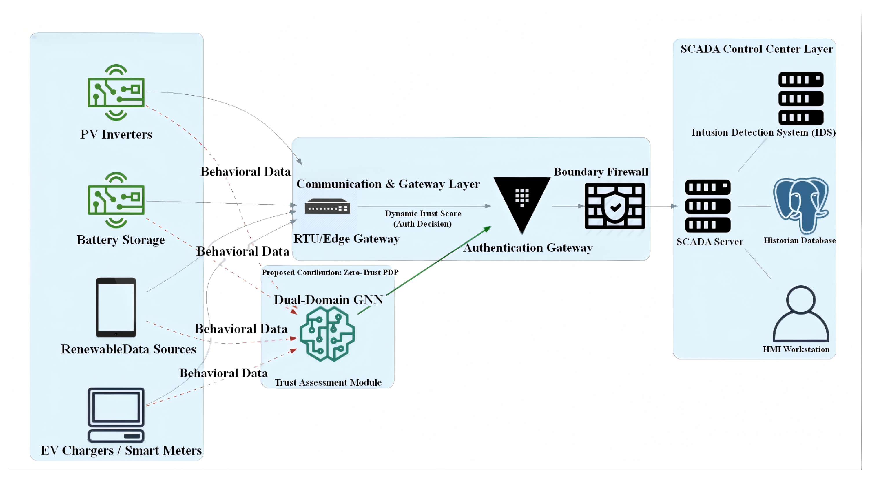Figure 2 presents the overall architecture of the proposed method and illustrates how behavioral perception, representation learning, relational modeling, and trust decision interfaces are integrated.

Each terminal is modeled as a node observed over discrete time windows. During each window, heterogeneous behavioral signals are collected from multiple sources, covering network traffic statistics, operational environment indicators, and hardware or event measurements at the kernel level. These observations jointly characterize terminal behavior from complementary perspectives. Relying on a single observation layer, such as network traffic alone, provides limited visibility into execution anomalies that manifest primarily at the host or system level, which motivates the use of multidimensional behavioral perception in the proposed architecture.

The collected behavioral features form a high dimensional and partially redundant representation. Direct aggregation of heterogeneous features increases dimensionality and noise, which complicates relational reasoning and degrades generalization. The architecture therefore incorporates a learned feature encoding component that transforms raw multisource observations into compact representations while preserving discriminative behavioral patterns relevant to trust assessment. This design choice reflects the assumption that effective trust inference depends on capturing intrinsic behavioral structure rather than raw feature magnitude.

Beyond individual behavior, terminal trust states exhibit dependency across nodes. Distributed terminals communicate and interact through network connections, and coordinated or lateral attack behaviors can induce correlated risk patterns across multiple nodes. Modeling terminals as independent entities fails to capture such collective effects. The proposed architecture addresses this dependency by explicitly representing relationships between terminals and performing relational reasoning over data structured as graphs.

Relationships between terminals are not limited to explicit communication links. Terminals that exhibit similar behavioral patterns may share latent risk characteristics even in the absence of direct interaction. The architecture therefore distinguishes between two complementary relational views: a topological view derived from observed communication relationships and a feature view derived from behavioral similarity among terminals. These views encode different aspects of dependency and are jointly incorporated into the trust assessment process.

Based on the learned terminal representations and relational reasoning results, the architecture produces a trust score for each terminal that reflects both individual behavioral risk and contextual influence from related nodes. The trust score serves as an intermediate decision variable that is subsequently mapped to discrete trust levels and associated access permissions, enabling granular and adaptive access control for distributed power grid terminals. Subsequent subsections detail the specific representation learning mechanisms, graph construction strategies, and optimization objectives that realize this architecture.

4.2. Multisource Behavioral Feature Encoding

Behavioral observations collected from distributed terminals exhibit both diversity and structural complexity. Network traffic reflects external interaction patterns, operational environment indicators capture execution load and resource usage, and hardware or events at the kernel level expose system activity at a low level. Each source emphasizes a different aspect of terminal behavior, and none of them alone provides a complete characterization of terminal trustworthiness. When these heterogeneous signals are jointly considered, the resulting feature space becomes high dimensional and partially redundant, which poses challenges for both representation learning and subsequent relational modeling.

The feature encoding strategy adopted in this work is designed to address two closely related objectives. One objective is to integrate heterogeneous behavioral signals into a unified representation that preserves patterns relevant to trust while suppressing noise and redundancy. The other objective is to control representation dimensionality so that reasoning based on graphs over large populations of terminals remains computationally feasible. 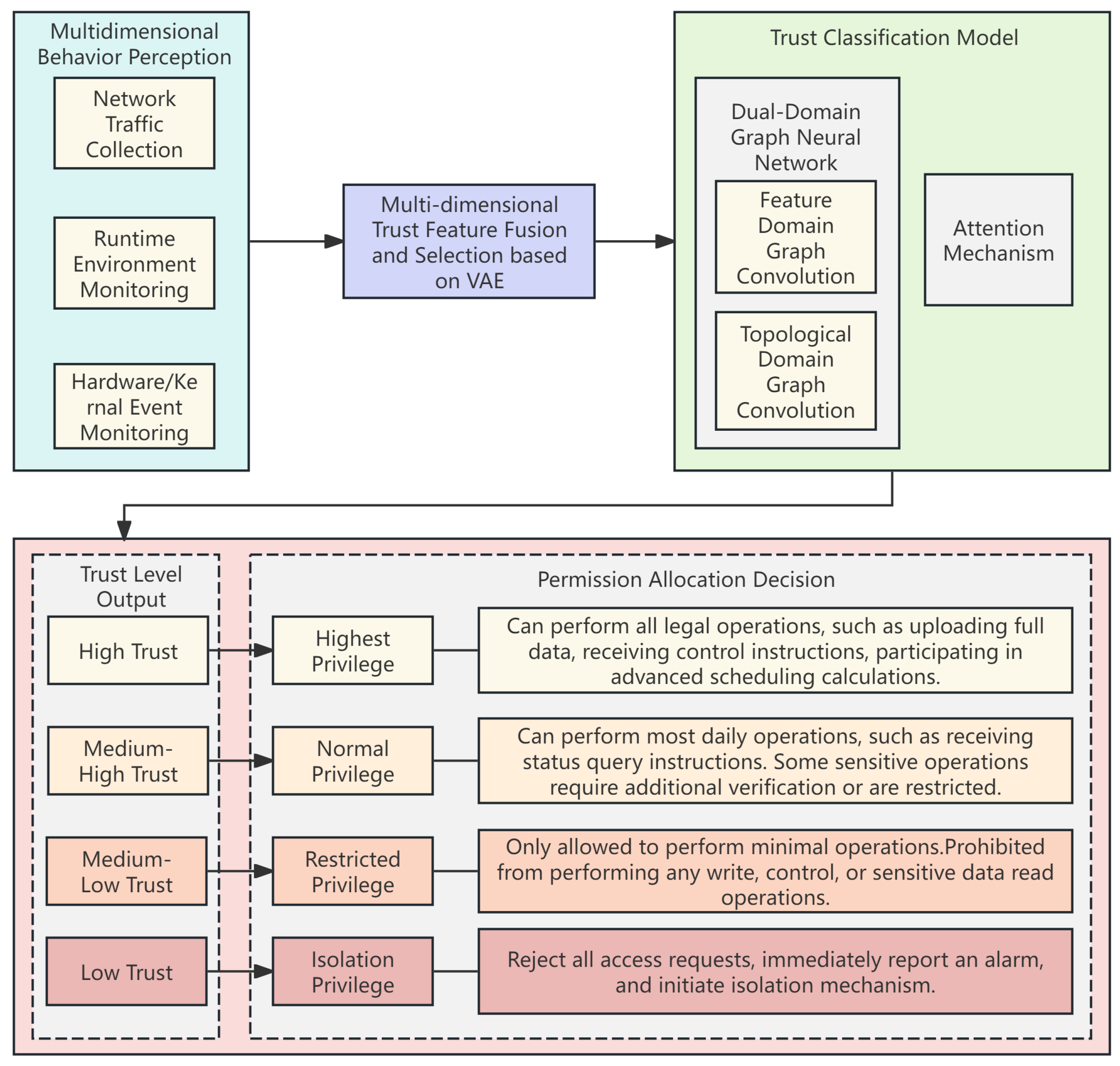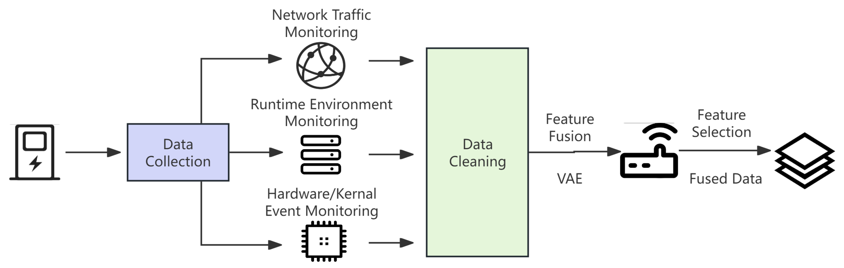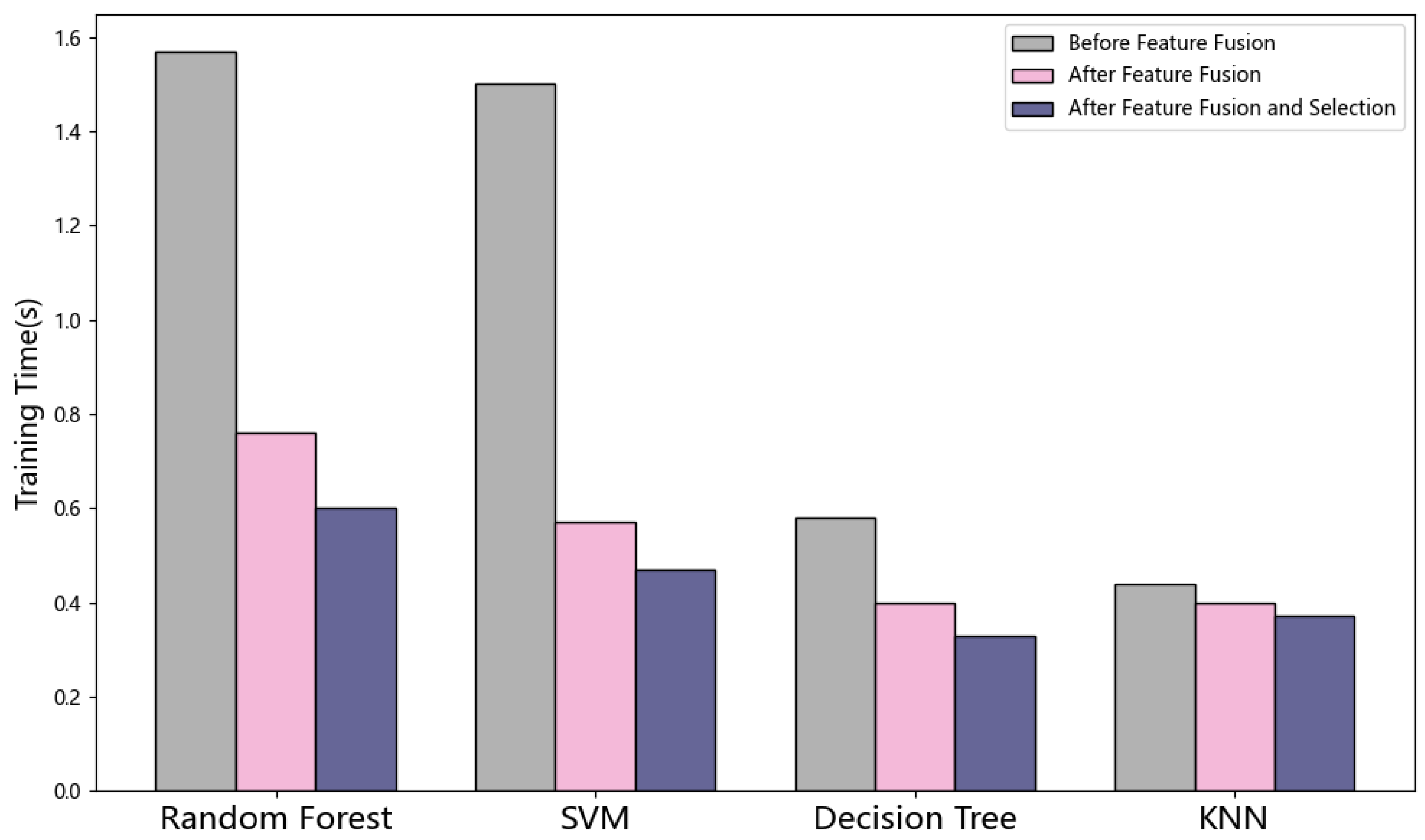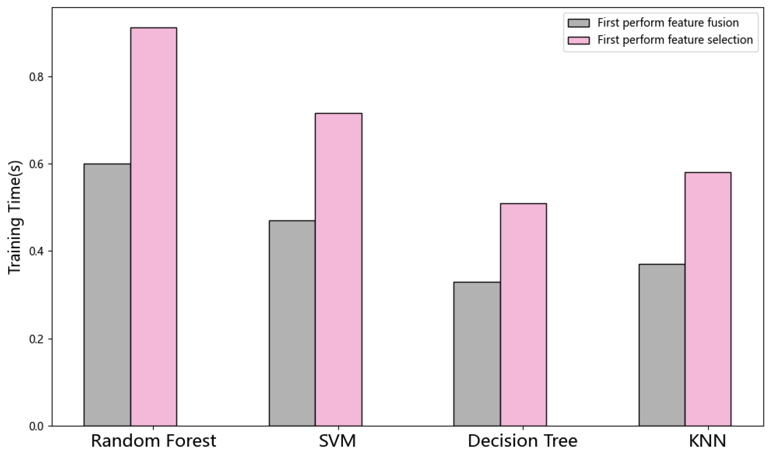Figure 3 provides a structural overview of the feature fusion and selection process used to satisfy these objectives.

As illustrated in Figure 3, the encoding process begins with multisource behavioral perception and progresses toward increasingly compact representations. The figure does not depict a rigid processing pipeline, but rather summarizes how raw observations are progressively transformed into representations suitable for relational learning. Early stages focus on establishing a consistent numerical feature space, while later stages emphasize representation compression and discriminative refinement. This separation reflects the design choice to decouple data normalization from representation learning, avoiding premature assumptions about feature relevance.

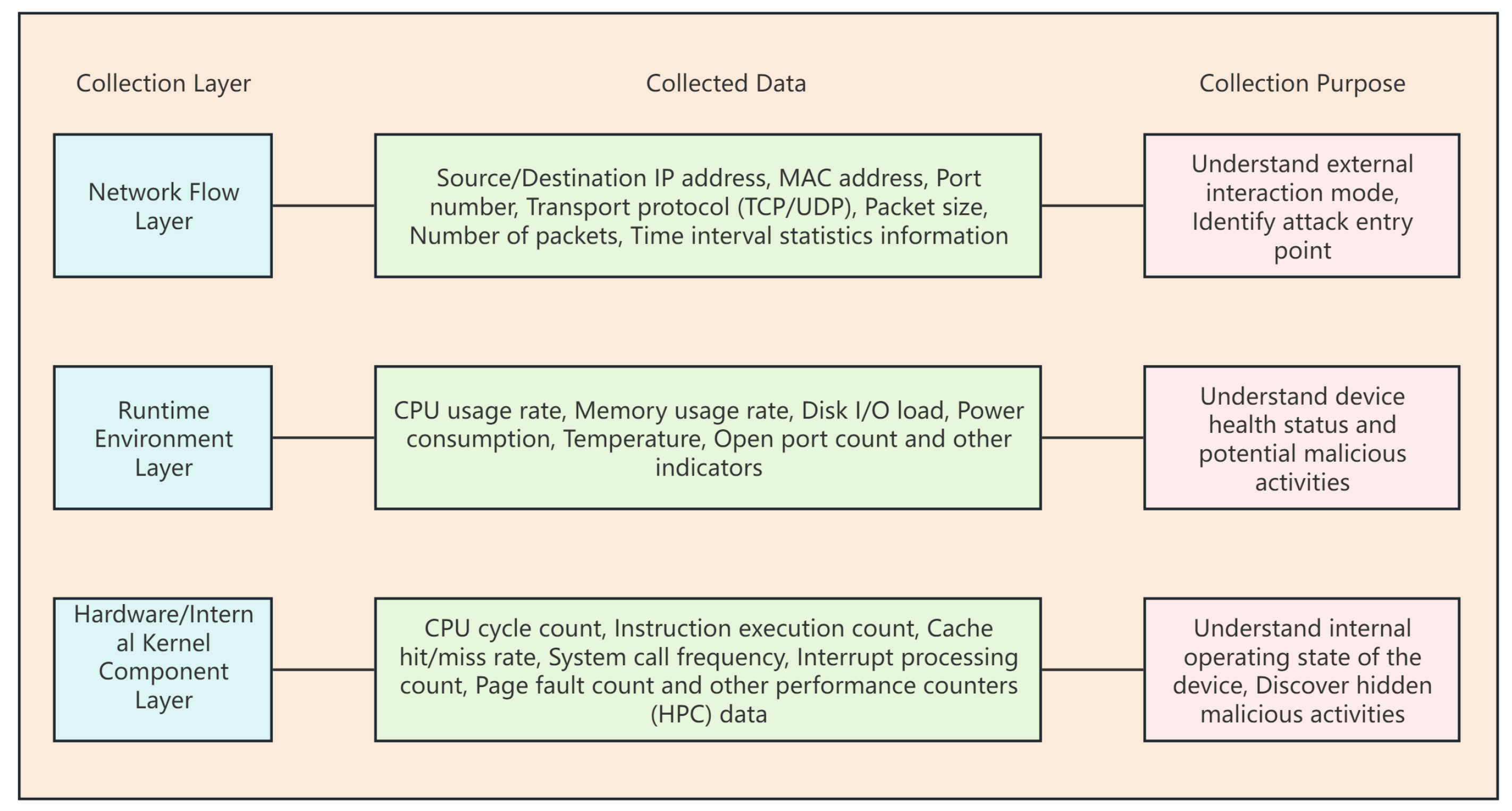
The sources of behavioral observations are summarized in Figure 4. Network traffic features capture communication behavior at the protocol and flow level, operational environment features describe runtime resource consumption, and events at the hardware or kernel level provide visibility into system internals that are weakly expressed at higher layers. These sources are collected within aligned observation windows and jointly characterize terminal behavior under both benign and adversarial conditions.

Raw observations from these sources are first preprocessed to ensure numerical consistency and stability. Invalid records are removed, uninformative or constant features are filtered, and categorical fields are transformed into numerical representations. This preprocessing stage does not attempt to manually optimize feature utility. Its role is to establish a stable input space for representation learning while minimizing bias introduced by handcrafted feature engineering.

To integrate the heterogeneous behavioral features into a compact representation, a variational autoencoder is employed. Direct concatenation of preprocessed features expands dimensionality and mixes signals with different statistical properties, which can obscure latent behavioral structure and amplify noise. The variational formulation introduces a continuous latent space that regularizes representation learning and encourages smoothness across samples. Let x denote the preprocessed feature vector associated with a terminal and let z denote its latent representation. The variational objective maximizes the Evidence Lower Bound (ELBO), formulated as:

$$logp\left(x\right)\ge {\mathbb{E}}_{z\sim q\left(z\right|x)}[logp\left(x\right|z)]-D_{\mathrm{KL}}(q\left(z\right|x)\parallel p\left(z\right)),$$

(1)

where ${\mathbb{E}}_{z\sim q\left(z\right|x)}$ denotes the expectation over the latent variable z sampled from the approximate posterior $q\left(z\right|x)$ produced by the encoder, and $p\left(x\right|z)$ denotes the likelihood of the reconstruction generated by the decoder. The Kullback-Leibler divergence term,

$$D_{\mathrm{KL}}(q\left(z\right|x)\parallel p\left(z\right))=\int q\left(z\right|x)log{\displaystyle \frac{q\left(z\right|x)}{p\left(z\right)}}dz,$$

(2)

constrains the learned latent distribution toward the prior $p\left(z\right)$ and limits overfitting to idiosyncratic variations in individual terminals. This regularization is critical for ensuring that latent representations remain comparable across devices and time windows.

In practice, to compute the Kullback-Leibler divergence term analytically, we assume the prior distribution $p\left(z\right)$ is a standard multivariate isotropic Gaussian, i.e., $p\left(z\right)=\mathcal{N}(\mathbf{0},\mathbf{I})$. The approximate posterior $q\left(z\right|x)$ is modeled as a multivariate Gaussian with a diagonal covariance matrix, formulated as $q\left(z\right|x)=\mathcal{N}(\mathit{\mu },\mathrm{diag}\left({\mathit{\sigma }}^2\right))$. To ensure numerical stability and guarantee that the variance remains strictly positive during implementation, the encoder network is designed to output the mean vector $\mathit{\mu }$ and the logarithmic variance vector $\mathit{v}=log\left({\mathit{\sigma }}^2\right)$. Under these standard distribution assumptions, the general integral form in Equation (2) can be analytically simplified into the following closed form expression:

$$D_{\mathrm{KL}}(q\left(z\right|x)\parallel p\left(z\right))=-{\displaystyle \frac{1}{2}}\sum _{j=1}^d\left(1+v_j-{\mu }_j^2-exp\left(v_j\right)\right),$$

(3)

where d is the dimensionality of the latent space, and ${\mu }_j$ and $v_j$ are the j-th elements of the mean vector $\mathit{\mu }$ and the logarithmic variance vector $\mathit{v}$, respectively. Here, the actual variance is naturally constrained to be positive as ${\sigma }_j^2=exp\left(v_j\right)$. This closed form loss is directly optimized during training.

The encoder is implemented as a multilayer perceptron comprising two layers with hidden dimensions 64 and 32 and ReLU activations. It outputs the parameters of the latent distribution, namely the mean $\mu$ and logarithmic variance v. Latent samples are obtained using the reparameterization trick to enable optimization using gradients.The decoder mirrors the encoder structure and reconstructs the input features using a linear output layer. Training minimizes reconstruction error together with the KL regularization term. Adam is used as the optimizer and mean squared error is adopted to quantify reconstruction quality. Early stopping is applied to prevent overfitting, and training samples are shuffled across epochs to avoid sensitivity to sample ordering.

Not all preprocessed features are passed through the variational encoder. Certain fields are preserved outside the fusion stage because they serve as structural anchors in subsequent graph construction and node association. Transforming these fields in the latent space would introduce uncontrolled interactions that weaken their semantic role in relational modeling.The variational encoder is therefore applied only to the remaining behavioral dimensions, producing compact representations that function as node attributes in the trust model based on graphs.

After variational compression, the feature space is reduced from 242 dimensions to 76. While this reduction significantly decreases redundancy, the remaining dimensionality still imposes a nontrivial computational burden for graph convolution with multiple layers, where complexity scales with both node count and feature dimension. Consequently, a second stage selection is applied to retain the feature subset that contributes most to supervised discrimination. Feature importance is estimated using a Random Forest classifier trained on labeled data. For a given feature $X_i$, its impurity reduction importance is computed as

$$\mathrm{Imp}\left(X_i\right)=\sum _{t\in T}\Delta I(X_i,t),$$

(4)

where T denotes the set of split nodes using $X_i$, and $\Delta I(X_i,t)$ represents the impurity reduction achieved at split t. Aggregating across all trees yields the importance at the forest level:

$${\mathrm{Imp}}_{\mathrm{RF}}\left(X_i\right)={\displaystyle \frac{1}{\left|F\right|}}\sum _{f\in F}{\mathrm{Imp}}_f\left(X_i\right),$$

(5)

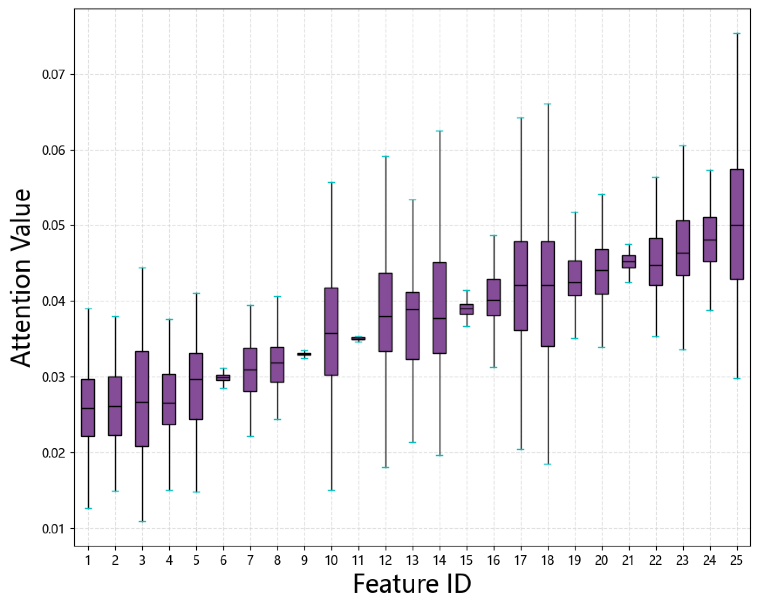
where F denotes the set of trees. To balance classification performance and computational cost, the optimal feature subset size was determined via 5-fold cross-validation. Based on the validation results, the top 25 features with the highest importance scores were retained. This selection achieves an additional 67% reduction relative to the 76-dimensional fused representation. The resulting compact feature vectors constitute the node attributes used for relational modeling across two domains in the following sections.

4.3. Dual Graph Construction

Relational dependency among terminals is represented using two complementary graphs defined over the same node set. Each node corresponds to a terminal observed within a time window and is associated with a compact behavioral feature vector produced by Section 4.2. Let $X\in {\mathbb{R}}^{n\times d}$ denote the node feature matrix, where n is the number of terminals and the i-th row $x_i$ is the feature vector of node i. Let $A\in {\{0,1\}}^{n\times n}$ denote the adjacency matrix derived from observed communication behavior.

Communication relationships are extracted from traffic records using identifiers such as source and destination MAC addresses. Although communication records are inherently directional, the relational encoder in this work is based on graph convolution with a symmetric adjacency. The adjacency matrix is therefore constructed as an undirected graph by setting $A_{ij}=1$ whenever communication between terminals i and j is observed in either direction within the time window, and $A_{ij}=0$ otherwise. This design retains connectivity information required for message passing while avoiding inconsistencies between directed edges and symmetric normalization in graph convolution.

The topology graph is defined as $G_T=(A,X)$, which encodes explicit interaction structure. This view is informative when correlated risk propagates along communication paths. However, communication alone does not capture latent similarity among terminals that exhibit comparable behavioral patterns without direct interactions.A second graph is therefore constructed to represent proximity in feature space, enabling relational reasoning over implicit behavioral dependencies.

The feature graph is defined as $G_F=(A_F,X)$, where $A_F$ is computed from a weighted combination of behavioral similarity and the topology prior. For nodes i and j, the relationship score is

$$A_F(i,j)=\omega S_{i,j}+(1-\omega )A_{ij},$$

(6)

where $\omega \in (0,1)$ controls the contribution of similarity and topology. The similarity term $S_{i,j}$ is computed using cosine similarity,

$$S_{i,j}=cos(x_i,x_j)={\displaystyle \frac{x_i·x_j}{\parallel x_i\parallel \parallel x_j\parallel }}.$$

(7)

Cosine similarity is used because it captures directional alignment in high dimensions and reduces sensitivity to feature magnitude. An edge is established in the feature graph when $A_F(i,j)$ exceeds a threshold $\tau$, which controls sparsity and the strength of coupling based on similarity. The threshold is treated as a hyperparameter and is selected on a validation split to balance relational coverage and noise amplification in message passing.

Algorithm 1 summarizes the construction of $A_F$.

Algorithm 1 Feature domain adjacency matrix construction

Require: Topology adjacency matrix A, feature matrix X, balance parameter $\omega$, threshold $\tau$

Ensure: Feature-domain adjacency matrix $A_F$

1: $A_F\leftarrow 0$ 2: for each pair of nodes $(i,j)$ do 3:    $S_{i,j}\leftarrow {\displaystyle \frac{x_i·x_j}{\parallel x_i\parallel \parallel x_j\parallel }}$ 4:    $r_{i,j}\leftarrow \omega S_{i,j}+(1-\omega )A_{ij}$ 5:    if $r_{i,j}>\tau$ then 6:        $A_F(i,j)\leftarrow 1$ 7:    end if 8: end for 9: Symmetrize $A_F$ by $A_F\leftarrow max(A_F,A_F^T)$

4.4. Dual-Domain Graph Encoder

Given $G_T$ and $G_F$, embeddings tailored to each domain are learned via graph convolution. Self loops are added to preserve node identity during message passing. For a generic graph with adjacency matrix A, the augmented adjacency and degree matrices are defined as $\tilde{A}=A+I$ and ${\tilde{D}}_{ii}={\sum }_j{\tilde{A}}_{ij}$. The propagation rule at each layer follows the normalized graph convolution operation.

$$H^{(l+1)}=\sigma \left({\tilde{D}}^{-{\displaystyle \frac{1}{2}}}\tilde{A}{\tilde{D}}^{-{\displaystyle \frac{1}{2}}}{H}^{\left(l\right)}{W}^{\left(l\right)}\right),$$

(8)

where $H^{\left(l\right)}$ denotes the node embedding at layer l, $W^{\left(l\right)}$ denotes trainable weights, and $\sigma (·)$ is a nonlinear activation.

In the feature domain, the encoder operates on $A_F$ and produces embeddings $\left\{Z_F^{\left(l\right)}\right\}$,

$$Z_F^{\left(l\right)}=\sigma \left({\tilde{D}}_F^{-{\displaystyle \frac{1}{2}}}{\tilde{A}}_F{\tilde{D}}_F^{-{\displaystyle \frac{1}{2}}}{Z}_F^{(l-1)}{W}_F^{\left(l\right)}\right),$$

(9)

with initialization

$$Z_F^{\left(0\right)}=X,$$

(10)

where ${\tilde{A}}_F=A_F+I$ and ${\tilde{D}}_F$ is the corresponding degree matrix. In the topology domain, the encoder operates on A and produces embeddings $\left\{Z_T^{\left(l\right)}\right\}$,

$$Z_T^{\left(l\right)}=\sigma \left({\tilde{D}}_T^{-{\displaystyle \frac{1}{2}}}{\tilde{A}}_T{\tilde{D}}_T^{-{\displaystyle \frac{1}{2}}}{Z}_T^{(l-1)}{W}_T^{\left(l\right)}\right),$$

(11)

where ${\tilde{A}}_T=A+I$ and ${\tilde{D}}_T$ is its degree matrix. The final domain embeddings are denoted by $Z_F$ and $Z_T$.

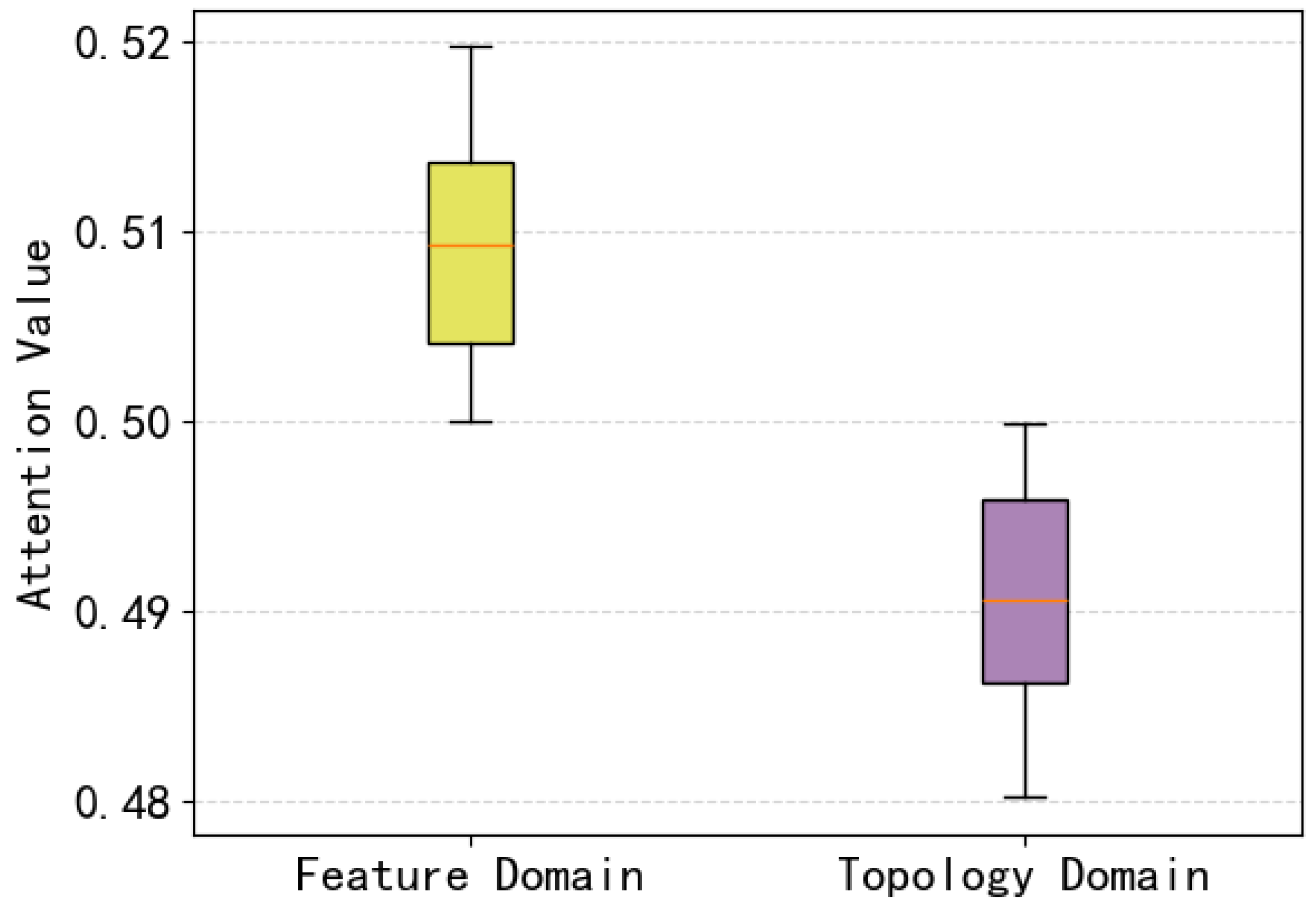
The two domains encode distinct dependency signals and are not expected to contribute equally across nodes or time windows. An attention mechanism at the node level is introduced to adaptively fuse $Z_F$ and $Z_T$ into a unified representation for trust inference. Let $z_f^i$ and $z_t^i$ be the final embeddings of node i in the feature and topology domains. Unnormalized attention scores are computed as

$${\xi }_f^i=q^T\sigma \left(W_{\alpha }{z}_f^i+b_{\alpha }\right),$$

(12)

$${\xi }_t^i=q^T\sigma \left(W_{\alpha }{z}_t^i+b_{\alpha }\right),$$

(13)

where $W_{\alpha }$ and $b_{\alpha }$ are trainable parameters and q is the attention vector. The normalized weights are obtained using a softmax applied in both directions,

$${\alpha }_t^i={\displaystyle \frac{exp\left({\xi }_t^i\right)}{exp\left({\xi }_t^i\right)+exp\left({\xi }_f^i\right)}},{\alpha }_f^i={\displaystyle \frac{exp\left({\xi }_f^i\right)}{exp\left({\xi }_t^i\right)+exp\left({\xi }_f^i\right)}}.$$

(14)

The fused embedding is then computed as

$$Z_i={\alpha }_t^i{z}_t^i+{\alpha }_f^i{z}_f^i.$$

(15)

Stacking ${\left\{Z_i\right\}}_{i=1}^n$ yields the unified embedding matrix $Z\in {\mathbb{R}}^{n\times d^{\prime }}$.

Algorithm 2 summarizes the embedding generation process in a form consistent with the above formulation.

Algorithm 2 Node embedding generation in the graph encoder for two domains

Require: Topology adjacency matrix A, feature adjacency matrix $A_F$, feature matrix X

Ensure: Unified node embedding Z

1: ${\tilde{A}}_T\leftarrow A+I$, ${\tilde{D}}_T\leftarrow \mathrm{deg}\left({\tilde{A}}_T\right)$ 2: ${\tilde{A}}_F\leftarrow A_F+I$, ${\tilde{D}}_F\leftarrow \mathrm{deg}\left({\tilde{A}}_F\right)$ 3: $Z_T^{\left(0\right)}\leftarrow X$, $Z_F^{\left(0\right)}\leftarrow X$ 4: for $l=1$ to L do 5:    $Z_T^{\left(l\right)}\leftarrow \sigma \left({\tilde{D}}_T^{-{\displaystyle \frac{1}{2}}}{\tilde{A}}_T{\tilde{D}}_T^{-{\displaystyle \frac{1}{2}}}{Z}_T^{(l-1)}{W}_T^{\left(l\right)}\right)$ 6:    $Z_F^{\left(l\right)}\leftarrow \sigma \left({\tilde{D}}_F^{-{\displaystyle \frac{1}{2}}}{\tilde{A}}_F{\tilde{D}}_F^{-{\displaystyle \frac{1}{2}}}{Z}_F^{(l-1)}{W}_F^{\left(l\right)}\right)$ 7: end for 8: for each node i do 9:     Compute ${\xi }_t^i,{\xi }_f^i$ using Equations (12) and (13) 10:    Compute ${\alpha }_t^i,{\alpha }_f^i$ using Equation (14) 11:    $Z_i\leftarrow {\alpha }_t^i{z}_t^i+{\alpha }_f^i{z}_f^i$ 12: end for 13: $Z\leftarrow [Z_1;\dots ;Z_n]$

4.5. Objective Function with Constraints Across Domains

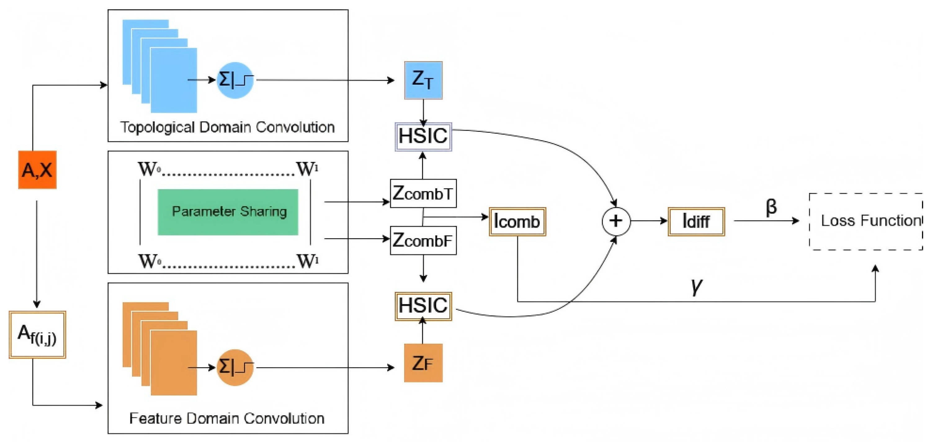
The unified embedding Z supports trust inference at the node level, but training benefits from an objective that explicitly controls how information is shared across domains. Embeddings from the feature and topology domains should capture compatible signals related to node labels, while retaining information specific to each domain that is not redundant. Figure 5 summarizes the constraint structure used in the objective design.

A commonality constraint encourages the two domains to preserve consistent pairwise similarity structure. Let $Z_{\mathrm{Tnor}}$ and $Z_{\mathrm{Fnor}}$ denote domain embeddings at a given layer after normalization. The similarity matrices are constructed as

$$S_T=Z_{\mathrm{Tnor}}{Z}_{\mathrm{Tnor}}^T,$$

(16)

$$S_F=Z_{\mathrm{Fnor}}{Z}_{\mathrm{Fnor}}^T.$$

(17)

The commonality loss is then defined as the Frobenius norm of their difference,

$${\mathcal{L}}_{\mathrm{comb}}={\parallel S_T-S_F\parallel }_F^2.$$

(18)

A complementarity constraint encourages the two domains to retain information specific to each domain by penalizing excessive dependence between each domain embedding and a combined embedding. The combined embedding is defined as

$$Z_{\mathrm{comb}}=\lambda Z_T+(1-\lambda )Z_F,$$

(19)

where $\lambda \in [0,1]$ is a mixing coefficient. Dependence is measured using the Hilbert-Schmidt Independence Criterion. Let $K_T$ and $K_{\mathrm{comb}T}$ be Gram matrices computed by an RBF kernel over $Z_T$ and $Z_{\mathrm{comb}}$, and let $J=I-{\displaystyle \frac{1}{n}}\mathbf{1}{\mathbf{1}}^T$ be the centering matrix. The HSIC term is computed as

$$\mathrm{HSIC}(Z_T,Z_{\mathrm{comb}})={\displaystyle \frac{1}{{(n-1)}^2}}\mathrm{tr}\left(K_{T}J{K}_{\mathrm{comb}T}J\right),$$

(20)

where the RBF kernel is

$$K(x_1,x_2)=exp\left(-{\displaystyle \frac{{\parallel x_1-x_2\parallel }^2}{2{\sigma }^2}}\right).$$

(21)

The corresponding dependence term for the embedding from the feature domain is computed analogously,

$$\mathrm{HSIC}(Z_F,Z_{\mathrm{comb}})={\displaystyle \frac{1}{{(n-1)}^2}}\mathrm{tr}\left(K_{F}J{K}_{\mathrm{comb}F}J\right).$$

(22)

The complementarity loss is defined as

$${\mathcal{L}}_{\mathrm{diff}}=\mathrm{HSIC}(Z_T,Z_{\mathrm{comb}})+\mathrm{HSIC}(Z_F,Z_{\mathrm{comb}}).$$

(23)

The trust inference task is implemented as supervised node classification. Let L denote the labeled node set, $Y_l$ denote the one-hot ground truth label of node l, and ${\widehat{Y}}_l$ denote the predicted label distribution. The cross entropy loss is

$${\mathcal{L}}_t=-\sum _{l\in L}\sum _{c=1}^C{Y}_{lc}log{\widehat{Y}}_{lc},$$

(24)

where $C=2$ for binary security-state classification. The total training objective is

$$\mathcal{L}={\mathcal{L}}_t+\gamma {\mathcal{L}}_{\mathrm{comb}}+\beta {\mathcal{L}}_{\mathrm{diff}},$$

(25)

where $\gamma$ and $\beta$ control the strength of the commonality and complementarity constraints.

The unified embedding Z is used for security state inference at the node level through a downstream classifier. The classifier consumes Z to produce label predictions $\widehat{Y}$ used in Equation (24). The specific classifier choice and its hyperparameters are treated as implementation details and are described in the experimental setup.

4.6. Trust Score Interpretation and Access Control Mapping

The trust assessment model produces, for each terminal node, a continuous confidence score that reflects the likelihood of the terminal being in a normal operational state. This score is derived from the output of a downstream classifier operating on the learned node embedding Z. Rather than treating the classification result as a binary decision, the proposed framework interprets the confidence score as a trust indicator that supports graded access control.

Let p denote the predicted probability that a terminal operates in an anomalous or normal state. This probability serves as the basis for trust evaluation and is mapped to discrete trust levels through predefined intervals. The mapping is implemented at the edge controller and functions as a decision interface between trust inference and access control enforcement. The use of discrete trust levels simplifies policy execution while retaining sensitivity to variations in model confidence.

Table 1. Trust level output and permission assignment.

Confidence Interval (p)	Trust Level	Permission Assignment
$1.0\ge p>0.9$	High trust	Maximum permissions
$0.9\ge p>0.7$	Medium–high trust	General permissions
$0.7\ge p>0.5$	Medium–low trust	Limited permissions
$p\le 0.5$	Low trust	Isolation permissions

summarizes the trust level definitions and their corresponding permission assignments. Higher confidence values indicate stronger evidence of benign behavior and result in broader access privileges, whereas lower confidence values trigger progressively stricter restrictions. Terminals assigned the lowest trust level are isolated from the system to prevent potential security risks.

The threshold values defining the trust intervals are selected to balance security sensitivity and operational continuity and can be adjusted according to deployment requirements. Once a trust level is determined, the edge controller enforces the corresponding access policy by exposing only the permissions associated with that level. This design confines potentially risky terminals to minimal functionality while allowing trusted terminals to participate fully in grid operations, thereby supporting adaptive zero-trust access control at a fine grain.

To demonstrate the practical application of our proposed trust assessment framework we designed a simulated validation scenario mapping the continuous trust scores to specific access control actions based on the permission assignment rules defined in Table 1. We selected four representative distributed terminals exhibiting distinct behavioral patterns. As illustrated in

Table 2. Simulated validation of access control mapping based on evaluated trust scores.

Terminal Node	Observed Behavior	Trust Score	Trust Level	Specific Control Action
EV Charger A	Standard charging telemetry	0.95	High trust	Grant unrestricted data exchange
EV Charger B	Occasional communication delays	0.85	Medium high trust	Allow routine telemetry and general commands
EV Charger C	High frequency request spikes	0.60	Medium low trust	Restrict to read only telemetry
EV Charger D	Known attack signature matched	0.12	Low trust	Isolate node and drop all packets

EV Charger A exhibits normal operational behavior yielding a trust score of 0.95 which falls into the High trust category and grants it Maximum permissions such as unrestricted data exchange within the grid. EV Charger B displays occasional communication delays resulting in a score of 0.85. This assigns it to the Medium high trust level where it receives General permissions allowing routine telemetry and standard commands. Conversely EV Charger C shows high frequency request spikes degrading its score to 0.60. Consequently the system downgrades it to the Medium low trust level applying Limited permissions that restrict it to read only telemetry to prevent potential denial of service attacks. Finally EV Charger D matches known attack signatures and receives a severely low score of 0.12 placing it in the Low trust category. This triggers Isolation permissions resulting in immediate node isolation and packet dropping. This simulated validation confirms that the continuous trust scores can be effectively translated into dynamic fine grained access control policies enhancing grid resilience.

5. Experiment Evaluation

5.1. Experimental Setup

The proposed method is evaluated on a dataset from the real world collected from electric vehicle charging infrastructure to assess its effectiveness under practical attack scenarios. All experiments are conducted on a unified workstation equipped with an Intel Core i9-10900K CPU @ 3.70 GHz, 64 GB of RAM, and a single NVIDIA GeForce RTX 3090 GPU (24 GB VRAM). The system runs Windows 10, with Python 3.8 and PyTorch 2.0.1 used as the primary implementation environment. Standard machine learning and scientific computing libraries are employed, and random seeds are fixed to ensure reproducibility across runs.

The experimental data are drawn from the CIC EV Charger Attack Dataset 2024 (CICEVSE2024), released by the Canadian Institute for Cybersecurity (CIC). Electric Vehicle Supply Equipment (EVSE) constitutes a critical edge node within modern distributed power grids, serving as a primary interface for external user access. Consequently, this dataset provides a representative view of edge access scenarios, capturing the communication protocols and attack vectors relevant to Zero-Trust verification.

Recognized for its rigorous construction and realistic testbed environment, this dataset has become a standard benchmark in smart grid security research. Its traffic patterns and attack vectors are representative of broader Internet of Energy (IoE) communications, ensuring that the proposed method is evaluated under realistic and challenging conditions. The dataset contains behavioral records of electric vehicle supply equipment operating under both benign conditions and a wide range of malicious attacks. It includes network traffic measurements, operational environment indicators, and event statistics at the kernel level, covering the three categories of behavioral observations considered in this work. More than twenty attack types are included, along with benign operation during both charging and idle states. Network traffic records contain source and destination MAC addresses that uniquely identify devices, enabling the construction of communication graphs between devices required for relational modeling.

Raw dataset entries contain redundant attributes, invariant features, and incomplete records that are unsuitable for representation learning. Data preprocessing therefore removes features whose values do not vary across samples and discards records with invalid or missing values.Attributes that are not numeric are converted into numerical representations to ensure compatibility with learning models. Beyond these normalization steps, no manual feature engineering is introduced.

The dataset contains millions of records, which makes direct use of the full dataset impractical. To balance computational cost and behavioral diversity while ensuring realistic evaluation, a differentiated sampling strategy is adopted. For the training set, samples are drawn such that the total number of benign samples matches the total number of malicious samples (1:1) to prevent classifier bias towards the majority class. However, to reflect the scarcity of attacks in real world power grid environments, the test set is constructed with an imbalanced distribution, consisting of approximately 90% benign samples and 10% malicious samples. This setup allows for a rigorous assessment of the False Positive Rate (FPR) and model robustness under conditions of low attack prevalence.

Graph encoders in both the feature domain and topology domain adopt a graph convolutional architecture with two layers, with hidden dimensions set to 128 and 256, respectively. ReLU is used as the activation function, and dropout with a rate of 0.5 is applied to mitigate overfitting. Model parameters are optimized using the Adam optimizer, with learning rates selected from the range $[{10}^{-4},5\times {10}^{-4}]$. Weight decay coefficients are set to $5\times {10}^{-3}$ and $5\times {10}^{-8}$ to stabilize training.

In the construction of the feature domain graph, the balance parameter $\omega$, which regulates the balance between feature similarity and the topology prior, is optimized within the range $[0,1]$ based on validation set performance. The edge threshold $\tau$, determining the sparsity of the adjacency matrix for the feature domain, is treated as a hyperparameter and tuned on a validation split. Specifically, a grid search over $\tau \in \{0.3,0.4,0.5,0.6,0.7\}$ is performed, and the selected optimal value is applied consistently across all reported experiments. Similarly, the coefficients $\gamma$ and $\beta$, associated with the commonality and complementarity constraints, are tuned via validation to achieve an optimal balance between supervised classification accuracy and regularization across domains.

The learned node embeddings serve as inputs to a downstream classifier for security state inference. In the current implementation, a support vector machine is trained on the embeddings to perform binary classification between benign and anomalous terminal states. Classifier hyperparameters are selected on a validation split and kept fixed across comparative experiments.

The security state classification task is evaluated as a binary classification problem. Performance is measured using accuracy (ACC), defined as the proportion of correctly classified terminal nodes. Accuracy is chosen as the primary evaluation metric because the dataset is balanced through stratified sampling and the trust decision logic relies on confidence-based segmentation rather than cost sensitive classification. All reported results are obtained by averaging performance over multiple runs with different random splits to reduce variance introduced by sampling and initialization.

5.2. Analysis of Feature Encoding and Computational Efficiency

To validate the efficacy of the proposed multidimensional feature encoding strategy, we analyzed the impact of fusion based on Variational Autoencoders (VAE) and selection based on Random Forests (RF) on feature distribution, classification accuracy, and training efficiency. The fusion using VAE reduces the input dimensionality from 242 raw features (covering hardware events, network traffic, and environmental metrics) to 76, achieving a compression ratio of approximately $70\%$. To visualize the distributional shift, we employed t-SNE to project the feature space. The visualization indicates that while the absolute spatial distribution changes due to latent mapping, the separability between benign and malicious samples is preserved and, in some clusters, enhanced. This suggests that the VAE effectively filters redundancy while retaining discriminative behavioral patterns.

We evaluated four standard classifiers—Random Forest (RF), Support Vector Machine (SVM), Decision Tree (DT), and K-Nearest Neighbors (KNN)—on datasets processed at different stages: (1) post VAE fusion only, and (2) post fusion followed by RF-based selection. As shown in

Table 3. Comparison of classification accuracy before and after feature selection (Test Set Ratio: 40%).

Dataset Stage	Random Forest	SVM	Decision Tree	KNN
After Fusion (Before Selection)	0.8467	0.8313	0.8538	0.8447
After Fusion + Selection	0.8503	0.8345	0.8553	0.8490

, the classification accuracy remains statistically stable across stages, with variations not exceeding $0.1\%$. This confirms that the dimensionality reduction process preserves the information entropy required for accurate trust assessment without introducing information loss.

A critical objective of feature encoding is to minimize computational overhead for real time edge deployment. Figure 6 illustrates the training time required for convergence. The combination of feature fusion and selection significantly accelerates model training; notably, the Random Forest classifier exhibited a $50.96\%$ reduction in training time. We further investigated the sequential order of the encoding pipeline by comparing fusion followed by selection against selection followed by fusion. While both orders maintain comparable accuracy, the proposed “Fusion then Selection” strategy yields a more compact feature set.

Table 4. Comparison of final feature counts under different processing sequences.

Processing Sequence	Initial Features	Final Features
Selection first, then Fusion	242	38
Fusion first, then Selection (Proposed)	242	25

compares the final feature counts resulting from different processing sequences. Performing feature fusion first results in 25 final features, whereas performing selection first results in 38 features. This difference arises because performing selection first on raw data with high dimensionality is less aggressive than selecting from the latent representations generated by the VAE.

Consequently, the impact of this sequence on time performance and accuracy was analyzed. As shown in Figure 7, the proposed order (Fusion first) further reduces training time due to the lower dimensionality. Meanwhile,

Table 5. Accuracy comparison of the final dataset generated by different processing sequences.

Sequence	Random Forest	SVM	Decision Tree	KNN
Selection first, then Fusion	0.8505	0.8343	0.8558	0.8487
Fusion first, then Selection	0.8503	0.8345	0.8553	0.8490

demonstrates that the classification accuracy remains consistent regardless of the sequence (e.g., $0.8503$ vs. $0.8505$ for RF). Therefore, the proposed framework adopts the sequence of fusion followed by selection to maximize information density and computational speed without compromising detection reliability.

5.3. Ablation Studies and Parameter Sensitivity

To verify the contribution of individual modules within the Dual Domain Graph Neural Network (DD-GCN) and assess its robustness, we conducted comprehensive ablation studies followed by a parameter sensitivity analysis. We first evaluated five variants of the proposed model to quantify the impact of the dual domain architecture and the specific constraint mechanisms. As summarized in

Table 6. Ablation study of DD-GCN components and constraints (Label Rate: 60%).

Model Variant	Key Components	Accuracy (%)	FPR (%)	Recall (%)	Precision (%)	F1-Score (%)
Topology-only Baseline	Graph Conv (Topology only)	95.13	4.82	85.60	87.90	86.73
Dual-Domain (DD) Base	DD-GCN w/o Constraints	95.57	4.25	88.80	86.40	87.58
DD + Complementarity	DD-GCN + ${\mathcal{L}}_{\mathrm{diff}}$	95.96	3.10	87.50	89.70	88.59
DD + Commonality	DD-GCN + ${\mathcal{L}}_{\mathrm{comb}}$	96.49	3.45	90.50	89.20	89.85
DD-GCN (Proposed)	DD-GCN + ${\mathcal{L}}_{\mathrm{comb}}$ + ${\mathcal{L}}_{\mathrm{diff}}$	96.84	2.15	91.93	92.15	92.04

, the complete DD-GCN model achieves the highest accuracy of 96.84% at a 60% label rate. Since relying solely on accuracy is insufficient for a comprehensive security evaluation, we additionally incorporated False Positive Rate, Recall, Precision, and F1 score into our assessment. The complete DD-GCN model attains a Precision of 92.15%, a Recall of 91.93%, an F1 score of 92.04%, and notably reduces the False Positive Rate to 2.15%. Maintaining a low False Positive Rate combined with high Recall is critical in power grid environments to effectively detect threats without erroneously interrupting normal terminal operations. The results demonstrate a clear performance hierarchy: the dual domain architecture consistently outperforms the baseline based only on topology (95.13%) which yields a significantly higher False Positive Rate of 4.82% and lower Recall of 85.60%, validating the hypothesis that integrating physical communication topology with behavioral similarity provides complementary views for trust inference. Furthermore, removing either the commonality constraint (${\mathcal{L}}_{\mathrm{comb}}$) or the complementarity constraint (${\mathcal{L}}_{\mathrm{diff}}$) leads to performance degradation across all evaluation metrics especially causing an unwanted increase in the False Positive Rate. This indicates that explicitly enforcing shared consistency and distinctiveness specific to each domain is crucial for preventing the model from overfitting to a single relational view.

Having established the structural superiority of the model, we examined the internal decision making process through the adaptive attention mechanism. This mechanism dynamically weights the importance of node embeddings derived from the feature and topology domains. As illustrated in Figure 8, we observe a slight skew in attention distribution towards the feature domain. This aligns with the intuition that intrinsic device behavior captured by the feature domain serves as the primary indicator of compromise, while topological propagation acts as a contextual reinforcer. Beyond weighting at the domain level, Figure 9 depicts the nonuniform attention weights assigned to specific latent features. This confirms that the network successfully prioritizes critical security indicators over irrelevant noise, significantly enhancing the interpret ability of the trust assessment. As further observed from the distribution in Figure 8 this adaptive skew provides a critical analytical insight for security applications. It inherently prevents the model from unfairly penalizing benign nodes simply because they are physically adjacent to infected ones thereby effectively reducing false positive rates in dense network segments. Furthermore the specific weight assignments depicted in Figure 9 reveal that the network acts as an implicit feature selector. By actively suppressing irrelevant background fluctuations the model fundamentally reduces the risk of overfitting to coincidental noise and provides security analysts with highly actionable forensic evidence.

We further investigated the sensitivity of the model to critical hyperparameters, specifically the balance parameter $\omega$ and the regularization coefficients. The balance parameter $\omega$ controls the construction of the adjacency matrix for the feature domain by modulating the balance between feature similarity and topological connections. As shown in Figure 10, classification accuracy exhibits a convex trend, peaking at $\omega \approx 0.6$. When $\omega$ is too low, the feature graph becomes isomorphic to the topology graph, negating the benefits of modeling across dual domains. Conversely, an excessively high $\omega$ introduces spurious connections based on coincidental feature similarities. It demonstrates that to effectively counter sophisticated topology spoofing attacks, the graph construction must be slightly biased towards behavioral similarity. This ensures that the learned relational graph reflects true operational dependencies rather than easily manipulated physical links. Thus, a moderate $\omega$ is optimal for preserving meaningful structural dependencies.

We further extended our sensitivity analysis to the edge threshold parameter $\tau$. As detailed in our methodology $\tau$ determines the sparsity of the feature domain adjacency matrix by filtering out weak relational links. We evaluated the model performance by varying $\tau$ across the predefined set of 0.3, 0.4, 0.5, 0.6 and 0.7. As illustrated in Figure 11 the experimental results demonstrate a distinct convex performance curve where the optimal classification accuracy and F1 score are achieved at $\tau$ equal to 0.5. When $\tau$ is set too low such as 0.3 the feature graph becomes excessively dense. This low threshold allows noisy and spurious connections to form between nodes with weak behavioral similarities which ultimately degrades the message passing efficiency and the overall detection accuracy. Conversely setting $\tau$ to an excessively high value like 0.7 results in an overly sparse graph. This high threshold aggressively prunes meaningful connections and isolates nodes thereby preventing the model from effectively aggregating complementary behavioral features. Therefore a moderate threshold of 0.5 strikes the best balance between relational coverage and noise suppression perfectly validating our parameter selection.

Finally, Figure 12 illustrates the performance variation with respect to the combination ($\gamma$) and difference ($\beta$) constraints. Both parameters follow a similar pattern where performance initially improves with increasing regularization but degrades beyond a certain threshold. Excessive values for $\gamma$ force the embeddings from both domains to be identical, resulting in a loss of unique information, while a large $\beta$ disrupts the primary classification objective. However, within the optimal range ($5\times {10}^{-9}$ to $10\times {10}^{-9}$ for $\beta$), the model demonstrates robust performance, particularly maintaining high accuracy even when labeled data is scarce (e.g., at a 15% label rate). It also means that effective cross domain learning requires a delicate equilibrium between consensus and diversity. Operating strictly within this optimal parameter range ensures that the model successfully enforces structural consistency across domains without derailing the primary classification gradient which perfectly explains its superior robustness under severe label scarcity.

5.4. Analysis of the Continuous Trust Level Output

To provide a more granular and realistic view of the model’s behavior under various operational conditions,

Table 7. Empirical Distribution of Trust Scores (p) Across Normal Operations and Various Graph Perturbation Scenarios.

Operational Status/Perturbation Type	Mean Score (p) ± Std	Classified as Abnormal ($\mathit{p}\le 0.5$)	Classified as Normal ($\mathit{p}>0.5$)
Normal Operation	$0.885\pm 0.112$	$2.15\%$ (False Positives)	$97.85\%$ (True Negatives)
Severe Topological Disruptions	$0.182\pm 0.095$	$98.45\%$ (Detected)	$1.55\%$ (Evaded)
Node Feature Corruptions	$0.365\pm 0.142$	$90.30\%$ (Detected)	$9.70\%$ (Evaded)
Stealthy Data Manipulations	$0.442\pm 0.198$	$86.12\%$ (Detected)	$13.88\%$ (Evaded)
Mixed/Camouflaged Anomalies	$0.291\pm 0.165$	$92.85\%$ (Detected)	$7.15\%$ (Evaded)

details the empirical distribution of the continuous trust level output p. We categorize the compromised scenarios based on how the underlying attacks manifest as data perturbations within the graph representation.

As shown in Table 7, during normal operations, the model outputs an average trust score of $0.885$, successfully mapping $97.85\%$ of the instances to a safe status ($p>0.5$). This aligns perfectly with the extremely low False Positive Rate ($2.15\%$) demonstrated in our ablation study.

When evaluating compromised nodes, the continuous score p exhibits varying sensitivities depending on the perturbation type, reflecting the inherent complexity of real world anomalies. For anomalies characterized by severe topological disruptions, the model demonstrates strong isolation capability, assigning a severely degraded average score of $0.182$ and capturing $98.45\%$ of the malicious nodes. In contrast, stealthy data manipulations present the greatest challenge, as their structural topology remains largely intact. Consequently, their average trust score rises to $0.442$, with the detection rate dropping to $86.12\%$. Interestingly, for mixed or camouflaged anomalies, the detection rate rebounds to $92.85\%$ (with an average score of $0.291$). This nonuniform behavior indicates that multidimensional perturbations often expose additional feature inconsistencies, which our Dual Domain mechanism effectively captures. Averaging across these diverse perturbation scenarios yields an overall macro recall of $91.93\%$, confirming that the framework consistently suppresses the trust scores of compromised terminals without needing to explicitly classify the underlying attack vectors.

5.5. Performance Evaluation and Comparative Analysis

To further evaluate the fundamental classification capability of the proposed DD-GCN framework, Figure 13 presents the normalized confusion matrix for the binary state evaluation. The confusion matrix further breaks down this performance: the model correctly identifies 98.1% of the actual Normal terminals, and achieves a high recall rate of 91.9% for the Abnormal category. The limited false negative rate confirms that the framework effectively minimizes the risk of treating an attacked terminal as benign.

Building upon this robust anomaly detection capability, the proposed framework further supports zero-trust access control at a fine granularity. Specifically, the model’s continuous confidence score $p\in [0,1]$ is directly mapped into four distinct trust tiers to facilitate flexible policy enforcement: High Trust ($p>0.9$), Medium High Trust ($0.7<p\le 0.9$), Medium Low Trust ($0.5<p\le 0.7$), and Low Trust ($p\le 0.5$).

Furthermore, to benchmark the effectiveness of the proposed DD-GCN in distributed terminal device security classification, we conducted extensive comparative experiments against baselines representing the state of the art. These baselines are categorized into Traditional Machine Learning (ML) methods, including SVM [30], Random Forest (RF [31]), Logistic Regression (LR [32]), LODA [33], LOF [34], and Deep Learning (DL) architectures, spanning structured models (LSTM, AE, CNN) and models based on graphs (GCN, GCN-FA [35]). All models were evaluated on the same dataset with engineered features, with DD-GCN parameters set to $\gamma =0.1$, $\beta =1\times {10}^{-8}$, and $\omega =0.54$.

Benchmarking against Traditional Algorithms.

Table 8. Performance Comparison with Traditional Machine Learning Algorithms (Label Rate: 60%).

Method	Accuracy (%)	Precision (%)	Recall (%)	F1-Score (%)
Logistic Regression [32]	78.25	65.40	61.30	63.28
SVM [30]	83.12	72.15	68.40	70.22
LODA [33]	81.45	69.80	66.50	68.11
LOF [34]	80.60	67.20	65.10	66.13
Random Forest [31]	86.45	75.30	71.80	73.51
DD-GCN (Ours)	96.84	92.15	91.93	92.04

presents the performance comparison with traditional ML algorithms. The proposed DD-GCN significantly outperforms these baselines across all metrics. Specifically, at a 60% label rate, DD-GCN achieves an accuracy of 96.84%, representing a relative improvement of approximately 10.39% over the traditional method with the best performance (Random Forest). More notably, in terms of the F1 score, DD-GCN (92.04%) surpasses the traditional baseline average by approximately 30%. This substantial performance gap highlights a fundamental limitation of traditional approaches: they treat data samples as independent and identically distributed (i.i.d.), thereby ignoring the critical communication topology and behavioral correlations between devices. By explicitly modeling these structural dependencies, DD-GCN effectively captures coordinated attack patterns that isolated classifiers inherently miss.

Evaluation against Deep Learning Architectures. We further compared DD-GCN with advanced deep learning models under varying label rates (15%, 30%, 60%), as summarized in

Table 9. Performance Comparison with Deep Learning Algorithms (%).

Label Rate	Metric	LSTM [39]	AE [40]	CNN [38]	GCN [36]	GCN-FA [37]	DD-GCN
15%	Accuracy	86.31	87.67	89.25	91.36	91.58	92.57
	F1-Score	85.14	84.09	83.37	85.31	85.94	88.27
30%	Accuracy	89.24	89.28	90.79	93.30	93.46	94.28
	F1-Score	87.35	86.42	84.24	89.53	88.37	90.47
60%	Accuracy	91.26	91.25	94.33	95.08	95.89	96.84
	F1-Score	89.72	88.69	86.58	92.15	91.93	92.04

. The results reveal a clear hierarchy in model capability. Models based on graphs (GCN [36], GCN-FA [37], DD-GCN) consistently outperform structured models without graph support (CNN [38], LSTM [39], AE [40]), reinforcing the necessity of relational modeling in power grid networks. Among the variants based on graphs, DD-GCN achieves the highest accuracy and F1 score across all label rates. Notably, even at a low label rate of 15%, DD-GCN maintains a high accuracy of 92.57%, demonstrating superior robustness in semi supervised settings compared to GCN-FA (91.58%) and standard GCN (91.36%).

The comparative advantage of DD-GCN over GCN-FA is particularly insightful. While GCN-FA enhances feature expression within a single topological domain, DD-GCN leverages an approach across dual domains that synthesizes physical connectivity (Topology Domain) with behavioral similarity (Feature Domain). The empirical results suggest that operating solely in the topological domain is insufficient when devices exhibit complex behavioral correlations. By integrating both domains via the adaptive attention mechanism, DD-GCN achieves a maximum relative accuracy growth of 5.58% over standard GCN, verifying that multidimensional structural constraints provide a more comprehensive view for security assessment.

Analysis of Precision and Recall. To further evaluate the model’s reliability in identifying threats, we analyzed the Precision Recall (PR) curves shown in Figure 14. In contexts critical to security, maintaining high precision at high recall levels is paramount to minimize false alarms while ensuring threat detection. The PR curves confirm that DD-GCN envelopes the curves of all baseline models, indicating a superior balance between precision and recall. Specifically, at a 90% precision threshold, DD-GCN improves recall by approximately 5.32% compared to GCN-FA. The distinct gap between DD-GCN and models without graph structures (CNN, LSTM, AE) further validates that extracting relational dependencies is as crucial as extracting individual feature patterns. The promising performance indicates that DD-GCN can extract the most relevant distributed terminal device feature information and effectively distinguish normal devices from compromised ones based on these fused structural insights.

5.6. Robustness and Computational Overhead Evaluation

5.6.1. Analysis of Cross Validation

To rigorously evaluate the robustness of the proposed Dual Domain GNN model and eliminate potential bias from a single random split for training and testing, we conducted cross validation with 10 folds on the dataset. The dataset was partitioned into 10 subsamples of equal size. In each iteration, one subsample was retained as the validation data for testing the model, and the remaining 9 subsamples were used as training data. This process was repeated 10 times, with each of the subsamples used exactly once as the validation data.

The average performance metrics, along with their standard deviations, are summarized in

Table 10. Performance Comparison using 10-Fold Cross-Validation (Mean ± Std).

Model	Accuracy (%)	Precision (%)	Recall (%)	F1-Score (%)
SVM	$83.12\pm 1.25$	$72.15\pm 1.30$	$68.40\pm 1.42$	$70.22\pm 1.32$
Random Forest	$86.45\pm 0.98$	$75.30\pm 1.05$	$71.80\pm 1.10$	$73.51\pm 1.04$
LSTM	$91.26\pm 0.85$	$87.50\pm 0.92$	$92.06\pm 0.88$	$89.72\pm 0.86$
GCN	$95.08\pm 0.62$	$93.10\pm 0.68$	$91.22\pm 0.65$	$92.15\pm 0.64$
Dual-Domain GNN	$96.84\pm 0.28$	$92.15\pm 0.35$	$91.93\pm 0.25$	$92.04\pm 0.31$

. As shown, our proposed model achieves an average accuracy of $96.84\%\pm 0.28\%$. The remarkably small standard deviation demonstrates that our Dual Domain GNN is highly generalized and maintains stable performance across different data subsets, proving its resilience to data variance compared to baseline methods.

5.6.2. Complexity and Quantitative Overhead

Trust assessment in real time within operational power systems requires strict control over computational overhead. To transparently evaluate this, we compare both the theoretical time complexity and the empirical hardware overhead of our proposed Dual Domain GNN against baseline methods.

Theoretically, the computational complexity of a standard GCN is bounded by $\mathcal{O}\left(\right(\left|V\right|+\left|E\right|)·d)$, where $\left|V\right|$ and $\left|E\right|$ denote the number of nodes and edges, and d is the feature dimension. In our proposed framework, message passing and aggregation are performed simultaneously on both the spatial domain graph ($G_s=(V_s,E_s)$) and the temporal domain graph ($G_t=(V_t,E_t)$). Therefore, the base complexity scales with the sum of the topological scales of both domains. However, to mitigate this, our framework utilizes a Variational Autoencoder (VAE) to compress the input features of high dimensionality into a compact latent dimension $d^{\prime }$ ($d^{\prime }\ll d$) prior to graph convolutions. Consequently, the final theoretical complexity is optimized to $\mathcal{O}\left(\right|V_s|+|E_s|+|V_t|+|E_t\left|\right)·d^{\prime }$.

To validate this theoretical derivation,

Table 11. Comparison of Theoretical Complexity, Inference Latency, and Memory Usage.

Model	Theoretical Complexity	Inference Latency (ms/Batch)	Memory Usage (MB)
SVM	$\mathcal{O}(N^2·D)$	$12.5$	$154.2$
Random Forest	$\mathcal{O}(K·NlogN)$	$8.4$	$210.5$
LSTM	$\mathcal{O}\left(W\right)$ per step	$48.6$	$465.8$
GCN	$\mathcal{O}\left(\right(\left|V\right|+\left|E\right|)·d)$	$18.2$	$315.4$
Dual-Domain GNN (Ours)	$\mathcal{O}\left(\right|V_s|+|E_s|+|V_t|+|E_t\left|\right)·d^{\prime }$	$24.8$	$382.6$

Note: N is the number of samples, D is the feature dimension, K is the number of trees, and W is the size of the weight matrix. $\left|V\right|$ and $\left|E\right|$ denote the number of nodes and edges, respectively. Subscripts s and t denote the spatial and temporal domains in our dual domain construction. d and $d^{\prime }$ represent the hidden dimensions before and after VAE compression.

summarizes the quantitative metrics, including average inference latency (in milliseconds per batch) and peak memory usage (in Megabytes). All empirical evaluations were conducted under the exact same hardware configuration (as detailed in Section 5.1) to ensure a fair comparison.

As shown in the table, baseline models exhibit varying computational balances. While traditional machine learning models like SVM and Random Forest operate with relatively low latency, their detection accuracy is often insufficient for complex grid environments. Conversely, sequence models like LSTM suffer from sequential processing bottlenecks, yielding the highest latency ($48.6$ ms) and memory consumption ($465.8$ MB). Our Dual Domain GNN introduces a slight computational overhead compared to the standard GCN based on a single graph ($24.8$ ms vs. $18.2$ ms) due to the dual graph construction. Nevertheless, facilitated by the VAE dimensionality reduction, the inference latency remains well within the strict response requirements from microseconds to milliseconds of modern smart grids, and the memory usage ($382.6$ MB) is highly manageable for practical deployment. This demonstrates that our model achieves a highly favorable and acceptable balance between superior trust assessment accuracy and operational overhead.

5.6.3. Scalability Analysis

To address the practical concerns of deploying our model in operational power systems at a large scale, we evaluate the scalability of the proposed Dual Domain GNN. Specifically, we investigate how the computational overhead, namely inference latency and memory usage, scales with an increasing number of grid terminals. In this experiment, we varied the number of terminal nodes ($\left|V\right|$) from 100 to 10,000 and recorded the corresponding performance metrics.

As illustrated in Figure 15, both inference latency and memory usage exhibit a manageable growth pattern that is nearly linear rather than an exponential increase as the network size expands. This favorable scaling behavior is primarily attributed to our feature dimensionality reduction using VAE and efficient graph processing strategies, which significantly reduce the computational burden of the dual domain construction. Consequently, the proposed model demonstrates robust scalability, proving its feasibility and efficiency for deployments in the real world within massive and distributed power grid environments.

6. Conclusions and Future Work

In this work, we proposed a novel zero-trust trust assessment framework for distributed power grid terminals, utilizing a Dual Domain Graph Convolutional Network (DD-GCN) to capture both individual behavioral anomalies and coordinated threats at the group level. By synthesizing heterogeneous data dimensions—including network traffic and kernel events—via a Variational Autoencoder and enforcing dual domain constraints, the model effectively mitigates the limitations of isolated detection methods. Comprehensive comparative experiments demonstrate that the proposed framework achieves a classification accuracy of 96.84% and an F1 score of 92.04%, significantly outperforming baselines representing the state of the art in machine learning and deep learning. These results validate that the fusion of physical topology with behavioral similarity provides a robust defense against complex lateral penetration attacks, offering a scalable and high-precision solution for securing the evolving smart grid infrastructure.

While our proposed dual domain graph neural network demonstrates high efficacy in identifying nodes with low trust, we acknowledge that the current trust granularity is relatively coarse and fundamentally operates akin to binary anomaly detection. In formulating our approach, we primarily drew inspiration from the classification-based paradigm of trust evaluation, as represented by several foundational works in distributed systems and IoT security [41,42,43]. Following this line of research, we treat trust assessment as a classification task designed to rapidly distinguish between benign and malicious entities. The primary objective of our framework is to enable dynamic access control rather than fine-grained intrusion detection. Consequently, our model focuses on macroscopic behavioral anomalies to quickly isolate compromised terminals, without classifying specific attack types, severities, or addressing extreme scenarios of class imbalance. We recognize that differentiating exact attack signatures falls strictly within the domain of specialized intrusion detection systems (IDS). Therefore, extending our classification-based trust model by integrating a dedicated IDS module to perform multiclass threat analysis under imbalanced conditions represents a crucial direction for our future research.

Along similar lines, our current data fusion strategy employs a single Variational Autoencoder (VAE) to merge data from multiple sources. While this unified design is lightweight and highly efficient for our current objective of macroscopic binary anomaly detection, we acknowledge that it may inadvertently dilute subtle, source-specific intrusion signals. For a framework strictly focused on rapid, binary trust classification, the single VAE provides a sufficiently compact representation. However, to advance towards fine-grained intrusion detection and more precise trust grading in the future, preserving the distinct boundaries of multimodal features is essential.

Furthermore, to explicitly distinguish the novelty of our proposed framework from existing multiview and dual domain graph neural network trust assessment methods, we emphasize our deep integration of heterogeneous terminal states. Conventional multiview graph networks predominantly rely on constructing alternate views from homogeneous network traffic data, which severely limits their visibility into underlying compromises at the device-level. Conversely, our framework constructs a topological domain representing the explicit physical and communication dependencies among power grid terminals, alongside a feature domain capturing intrinsic behavioral similarities. Crucially, these behavioral features are not merely network statistics but a synthesized representation of hardware events and kernel logs compressed via a variational autoencoder. This architectural design enables our model to identify sophisticated lateral penetration attacks where a compromised terminal might maintain normal network routing metrics but exhibit abnormal internal kernel behaviors. Consequently, our approach surpasses standard multiview methods by bridging the critical gap between macro-level network topology and micro-level terminal operating states within a zero-trust architecture.

To fully contextualize the value of our proposed solution within the broader landscape of smart grid security, it is essential to compare our behavior-based framework with other prominent decentralized paradigms. While blockchain technology is widely adopted in distributed power systems to ensure data immutability and decentralized consensus, our Dual Domain GNN trust framework offers distinct advantages for terminal assessment. First, blockchain primarily guarantees the cryptographic integrity of transactions and device identities, but it inherently lacks the capability to analyze complex behavioral anomalies in real time. An authenticated node that is subsequently compromised could still broadcast cryptographically valid but malicious data on chain. In contrast, our framework continuously models multidimensional behavioral features to dynamically assess the genuine trust status of terminals. Second, traditional blockchain consensus mechanisms introduce significant latency and computational overhead, which are often prohibitive for fine-grained monitoring of resource-constrained grid terminals in real time. Once trained, our GNN-based model provides low-latency inference, enabling continuous and responsive trust evaluation.

For future work, we recognize the complementary nature of these two technologies and plan to explore their integration. Specifically, our GNN-based framework could serve as an intelligent behavioral oracle that computes dynamic trust scores, while a lightweight consortium blockchain could be employed as a decentralized immutable ledger to securely log these trust assessments and audit trails across different power grid administrative domains. This hybrid architecture would simultaneously achieve precise threat detection in real time and secure historical traceability that is tamper proof.