A Hybrid LSTM-iTransformer Model with Data Augmentation for Battery State-of-Health Estimation

Abstract

Given the growing concern over the operational safety and long-term reliability of lithium-ion batteries, the accurate assessment of battery state of health (SOH) is of paramount importance. With the aim of elevating the SOH estimation exactitude and remedying the model degradation induced by data paucity, this paper proposes an SOH estimation method that integrates a data-augmentation strategy with a Long Short-Term Memory (LSTM)-iTransformer model. Specifically, multiple health characteristic factors characterizing the aging behavior are first extracted from the battery charge–discharge curves and incremental capacity (IC) curves, and the features that are highly correlated with the SOH are screened by a Pearson correlation coefficient analysis. Subsequently, the data augmentation technique is used to extend the degradation sample set. The LSTM-iTransformer model is trained based on the extended samples and evaluated on multiple performance metrics. A comparative analysis reveals a marked enhancement in predictive accuracy achieved by this method over the baseline model trained with the initial data, which validates the effectiveness of the data augmentation strategy in improving the performance of SOH estimation models. Additionally, in scenarios characterized by abundant data availability, the direct application of this model facilitates enhanced predictive precision.

1. Introduction

In response to climate change, the pursuit of green and low-carbon development has become a sustained imperative for nations worldwide. In recent years, lithium-ion batteries have played a role in many industries, driving the continuous development of related industries [1]. The safety of lithium-ion batteries has received widespread attention from people [2,3]. As the running time prolongs, lithium-ion batteries will be affected by various internal and external factors, leading to a gradual deterioration of battery health. This degradation may lead to performance degradation and, in some cases, catastrophic failures [4], thereby elevating safety risks such as thermal runaway [5]. Therefore, the accurate estimation of the state of health (SOH) of lithium-ion batteries is essential for improving the safety, reliability, and service life of battery systems [6].

Lithium-ion batteries serve as a critical energy storage medium, also in important domains including grid energy storage systems [7], aerospace technologies, and medical equipment [8]. Applications in these fields impose rigorous safety and reliability requirements on lithium-ion batteries, as even minor operational anomalies or performance deterioration can trigger severe consequences, including irreversible damage [9]. Consequently, developing precise and efficient methods for SOH estimation has emerged as a primary research focus, essential for ensuring operational stability and prolonging the service life [10]. Battery SOH is conventionally evaluated through two core parameters: capacity and internal resistance [11]. In this study, the SOH is defined based on capacity degradation, expressed as follows:

$$SOH={\displaystyle \frac{C_i}{C_{new}}}\times 100\%$$

(1)

where C_i denotes the current maximum available capacity of the battery, and C_new represents the rated capacity of the battery when new.

Current methodologies for estimating the SOH of lithium-ion batteries can be classified into four primary categories: direct measurement techniques [12], physics-based models [13], hybrid frameworks [14], and data-driven approaches [15]. Among these, data-driven methods have attracted growing research interest in recent years due to their exceptional modeling versatility and robust adaptability to diverse battery operating conditions. Direct measurement methods quantify battery SOH by assessing measurable physical parameters, including the capacity [16], electrochemical impedance spectroscopy [17], and internal resistance, and by IC analysis [18]. These techniques, characterized by their dependence on empirically observable quantities, exhibit simplified algorithmic architectures and enhanced interpretability, thereby achieving widespread adoption in laboratory environments [19]. Nevertheless, such approaches generally necessitate high-precision instrumentation and strictly controlled testing conditions, constraining their practical deployment in real-world applications—especially for online monitoring systems [20].

The physics-based modeling paradigm primarily encompasses three methodologies: equivalent circuit models, electrochemical models, and empirical formulations [21]. This approach constructs mathematical representations of battery dynamics by analyzing internal aging mechanisms to characterize operational behavior [22]. Compared to alternative techniques, physics-based models demonstrate enhanced transferability and interpretability, enabling parameter calibration across diverse battery chemistries and operating regimes [23]. Nevertheless, these models face significant challenges including computational intensity and complex parameterization requirements. Moreover, deviations between actual operating conditions and model assumptions may compromise the estimation robustness. Bodnar et al. developed a semi-empirical model incorporating simplified internal process representation and capacity regeneration effects, achieving computational efficiency while improving the SOH estimation accuracy in battery management systems [24]. Sangiri et al. proposed a perturbation-based diagnostic technique utilizing the discrete Fourier-transform analysis of voltage responses to specific-frequency current excitations, establishing quantifiable relationships between signal power metrics and aging parameters for SOH and remaining useful life (RUL) [25]. Ma et al. implemented a fractional-order equivalent circuit model with joint state estimation via adaptive genetic algorithm parameterization and multi-innovation unscented Kalman filtering, enabling a simultaneous high-accuracy SOC/SOH estimation [26].

The data-driven approach bypasses the need for physical modeling or mechanical analysis inside the battery, and directly learns the nonlinear mapping between battery features and the SOH from a large amount of operational data to achieve an accurate health state estimation. In related studies, Guan et al. proposed a predictive model for fast-charging lithium-ion batteries that extracted 52 domain-specific and 44 statistical features from the first 100 cycles, employed a BI-Mamba model to capture temporal dependencies, and used a feedforward neural network for early-life lifetime prediction [27]. However, it should be noted that increasing feature dimensionality also escalates model training costs. Consequently, concise yet efficient features are essential for feeding models. Hu et al. proposed a hybrid Variational Mode Decomposition-GRU (Gate Recurrent Unit, GRU)/LSTM network model for predicting the SOH and RUL of lithium-ion batteries [28]. Nevertheless, the Variational Mode Decomposition method incurs significant computational time when processing long-term sequential signals, substantially increasing the demands for computational resources and processing duration. Additionally, individual modules often exhibit deficiencies in robust feature extraction and mapping capabilities. To address these limitations, Chen et al. developed a framework employing an adaptive dilated convolution and Transformer backbone, which integrates parallel local convolutions with global attention mechanisms, optimized via weighted fusion [29]. The framework utilizes Kolmogorov–Arnold Networks for the final prediction, achieving an accurate battery SOH estimation. While this multi-module integration enhances the prediction accuracy, it concurrently amplifies the model complexity and introduces heightened risks of overfitting. Currently, many researchers have combined the strengths of data-driven methods with physical modeling approaches to achieve an effective SOH estimation. Ye et al. proposed the Physical-Information Feedforward Neural Network, which extracts key features from IC and differential temperature curves [30]. The monotonic relationship between the IC peak values and SOH is encoded as a physical constraint within the network, thereby improving both the interpretability and estimation accuracy. Lin et al. introduced a lightweight two-stage Physics-Informed Neural Networks model that accounts for the differences in battery chemistries [31]. Aging-related features were extracted from the post-charge relaxation voltage and IC curves, and relevant physical principles were incorporated into the loss function during training to improve the predictive performance.

To alleviate the data scarcity problem, a Time-Series Generative Adversarial Network (TimeGAN)-based augmentation strategy is adopted to enrich the degradation trajectory distribution while preserving temporal consistency. Beyond a simple data expansion, this strategy enhances the diversity of degradation patterns and improves the robustness of the subsequent model learning. More importantly, this study proposes a hierarchical LSTM-iTransformer architecture for SOH estimation. Unlike naive stacking approaches, the proposed framework functionally decomposes temporal modeling into two complementary stages. The LSTM module first performs local temporal smoothing and short-term dependency extraction, effectively suppressing high-frequency fluctuations and generating structured intermediate representations. These refined features are then fed into an improved Transformer (iTransformer), which captures long-range degradation dependencies through a global self-attention mechanism. By explicitly separating short-term dynamic filtering and long-term degradation trajectory modeling, the architecture addresses the multi-scale temporal characteristics inherent in battery aging processes. Compared with existing Transformer-based SOH estimation methods that directly apply attention mechanisms to raw time-series inputs, the proposed model introduces a structured feature reorganization stage before global modeling. This hierarchical temporal learning strategy enhances representation stability, improves attention reliability under limited data conditions, and strengthens the long-term degradation trend modeling capability.

Comprehensive experiments validate the effectiveness of both the TimeGAN-based data augmentation method and the proposed hierarchical LSTM-iTransformer architecture, demonstrating superior accuracy and robustness in battery SOH estimation tasks. The remainder of this paper is organized as follows: Section 2 introduces the publicly available NASA and CALCE battery datasets used in this study, detailing the extracted aging features and the applied data augmentation methods. Section 3 presents the architecture and design rationale of the proposed LSTM-iTransformer model. Section 4 provides an in-depth experimental analysis based on the public datasets, including a comparative evaluation of the model’s predictive performance on the NASA dataset before and after data augmentation, as well as benchmarking against other mainstream approaches. Finally, Section 5 concludes the paper and offers insights into potential directions for future research.

2. Data Processing

2.1. Dataset Selection

2.1.1. NASA Dataset

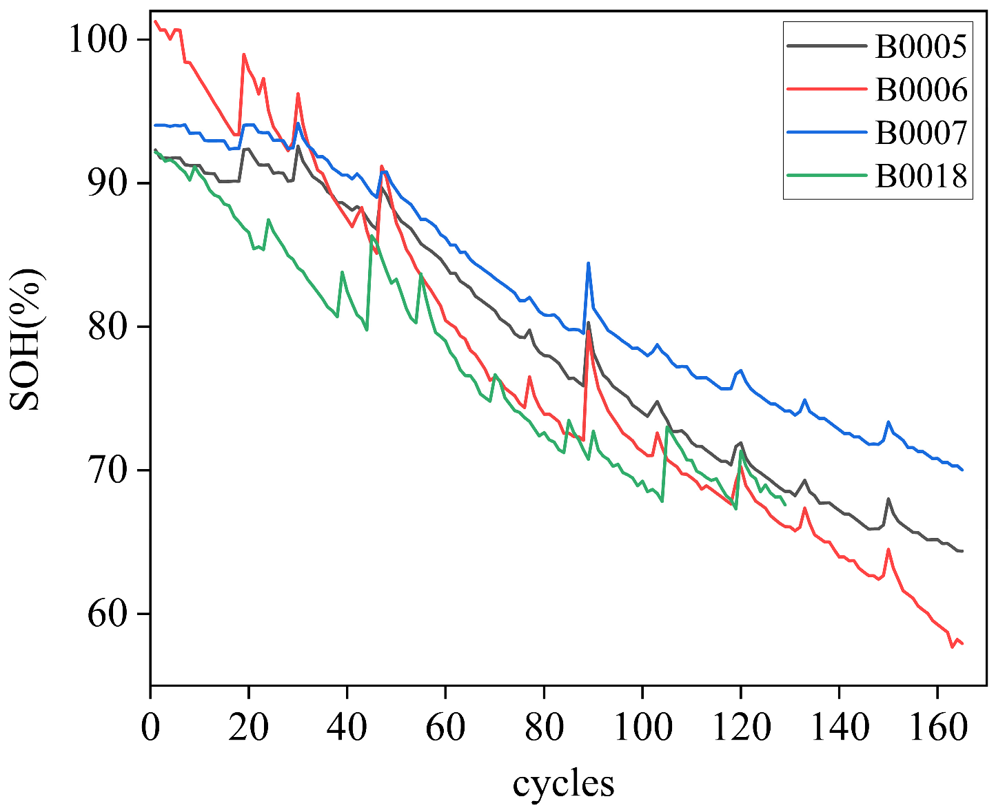
This investigation employs cycling data from the NASA lithium-ion battery dataset, which includes cells B0005, B0006, B0007, and B0018. All four cells were aged through continuous cycling in a controlled laboratory environment maintained at a constant temperature of 24 °C. Throughout the testing process, charging, discharging, and impedance measurements were systematically performed to monitor the degradation of battery performance over time and to analyze the deterioration patterns of internal battery parameters. Detailed specifications of the batteries and the corresponding test conditions are provided in

Table 1. Battery parameter information in the NASA dataset.

Battery	Rated Capacity	Charging Current	Discharging Current	Charge Cut-Off Voltage	Discharge Cut-Off Voltage
B0005	2 Ah	1.5 A	2 A	4.2 V	2.7 V
B0006	2 Ah	1.5 A	2 A	4.2 V	2.5 V
B0007	2 Ah	1.5 A	2 A	4.2 V	2.3 V
B0018	2 Ah	1.5 A	2 A	4.2 V	2.5 V

, while the capacity degradation trends across the battery cycle life are illustrated in Figure 1.

2.1.2. CALCE Dataset

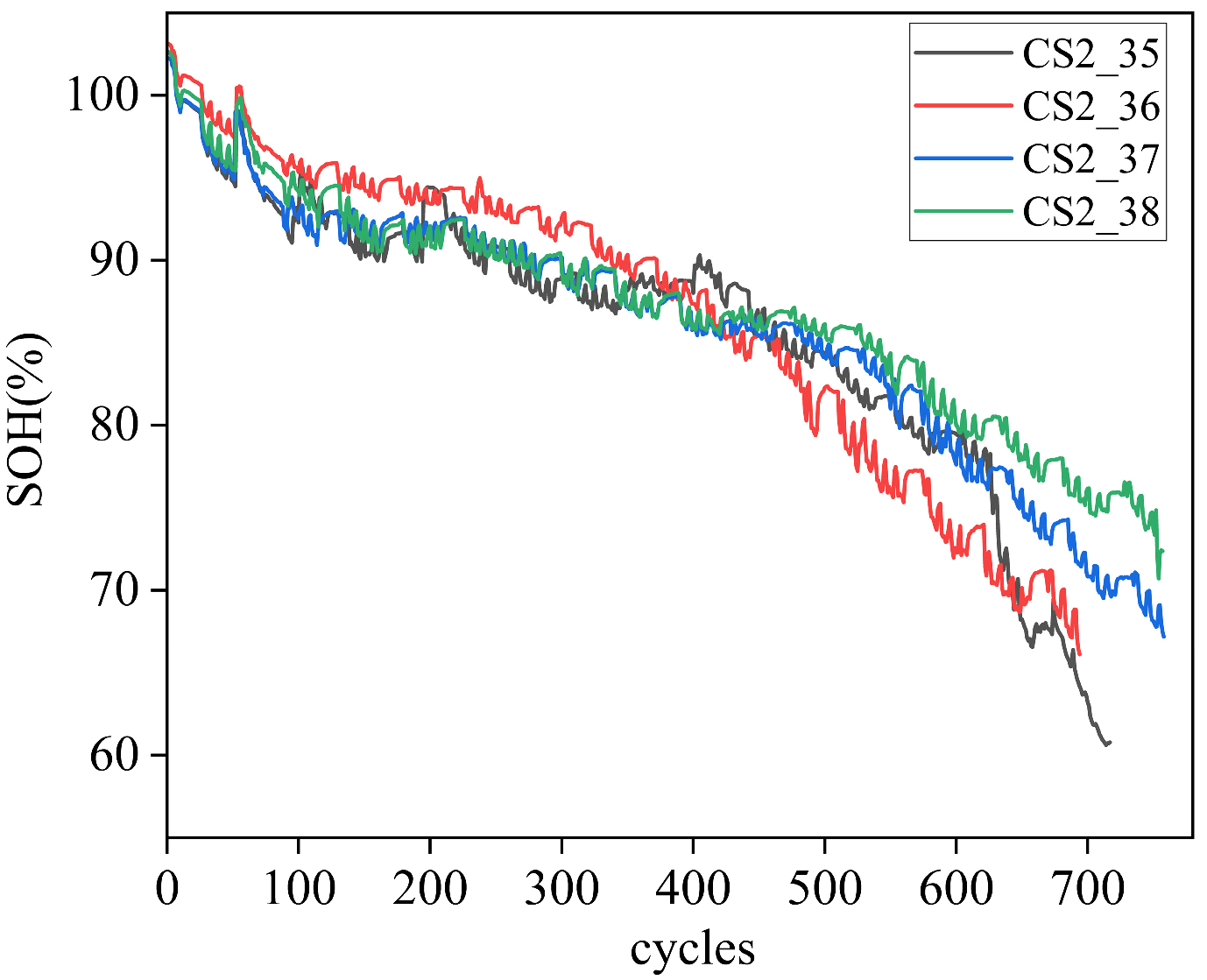
To further validate the proposed method, cycling data obtained from the CALCE battery research group were also employed in the experimental verification, including four datasets from the CS2 series designated as CS2_35, CS2_36, CS2_37, and CS2_38. During charging, a constant current is initially applied until the battery voltage reaches 4.2 V, after which the charging process transitions to a constant voltage mode maintained at 4.2 V. Charging is terminated once the current drops to 0.05 A. The battery is then discharged at a constant current until the voltage falls to 2.7 V, completing a full charge–discharge cycle. The battery performance data are recorded for each cycle, and multiple cycling experiments are conducted to capture the aging behavior. The detailed experimental parameters are summarized in

Table 2. Battery parameter information of the CALCE dataset.

Battery	Rated Capacity	Charge Cut-Off Voltage	Discharge Cut-Off Voltage
CS2_35	1.1 Ah	4.2 V	2.7 V
CS2_36	1.1 Ah	4.2 V	2.7 V
CS2_37	1.1 Ah	4.2 V	2.7 V
CS2_38	1.1 Ah	4.2 V	2.7 V

, while the capacity degradation trends over the battery lifespan are illustrated in Figure 2.

2.2. Feature Selection

Before feature extraction, it is essential to clarify the intrinsic relationship between battery aging mechanisms and observable charge–discharge characteristics. The SOH of a lithium-ion battery is fundamentally governed by capacity loss and internal resistance growth, which originate from the loss of active lithium, the loss of active material, and intensified polarization effects. These degradation mechanisms inevitably induce systematic variations in the voltage plateau behavior, charging time distribution, current attenuation dynamics, and differential capacity characteristics. Therefore, features derived from charge curves, discharge curves, and IC curves can serve as physically interpretable indicators that reflect the underlying electrochemical aging processes. The selection of feature factors in this study is thus guided not merely by statistical correlation, but by their mechanistic relevance to capacity fade and kinetic degradation. In this study, ten key feature factors (denoted as HF1 to HF10, detailed in

Table 3. The ten features associated with SOH extracted from charging and discharging.

Number	Feature Name
HF1	constant voltage charging time drop form 3.9 V and 4.1 V
HF2	constant current charging time
HF3	constant voltage charging time
HF4	constant voltage discharging time drop from 4.0 V and 3.9 V
HF5	current–time integral during the entire charging process
HF6	current–time integral during constant current charging
HF7	current–time integral during constant voltage charging
HF8	peak value of the IC curve
HF9	voltage corresponding to the IC peak
HF10	the ratio of constant current charging time to total charging time

) were extracted from the charge curve, discharge curve, and IC curve. Specifically, these features include the following: the constant voltage charging time drop from 3.9 V and 4.1 V (HF1), the constant current charging time (HF2), the constant voltage charging time (HF3), the constant voltage discharging time drop from 4.0 V to 3.9 V (HF4), the current–time integral during the entire charging process (HF5), the current–time integral during constant current charging (HF6), the current–time integral during constant voltage charging (HF7), the peak value of the IC curve (HF8), the voltage corresponding to the IC peak (HF9), and the ratio of constant current charging time to total charging time (HF10). Specifically, features related to the charging duration and current–time integration (HF2, HF5, and HF6) directly correspond to the reversible capacity, which is inherently consistent with the definition of the SOH. Features describing the constant voltage behavior and voltage interval duration (HF1, HF3, HF4, HF7, and HF10) reflect the polarization evolution and internal resistance growth, both of which are key manifestations of aging. Meanwhile, IC-curve-based features (HF8 and HF9) capture variations in electrochemical reaction kinetics and phase transition behavior, enabling the identification of active material loss and structural degradation.

By jointly incorporating these capacity-related, polarization-related, and kinetic-related indicators, the constructed feature set provides a multi-dimensional physical representation of battery degradation, thereby ensuring a strong interpretability and relevance to the SOH estimation. To further verify their quantitative relevance to the SOH, Pearson correlation coefficients were calculated to evaluate the linear dependence between each feature and the aging state. The battery degradation process typically exhibits an approximately monotonic trend during cycling. In this scenario, the Pearson correlation coefficient provides a reasonable and stable measure of correlation. The formula is as follows:

$$r={\displaystyle \frac{{\displaystyle {\sum }_{i=1}^n(H{F}_i-\overline{HF})(SO{H}_i-\overline{SOH})}}{\sqrt{{\displaystyle {\sum }_{i=1}^n{(H{F}_i-\overline{HF})}^2}}\sqrt{{\displaystyle {\sum }_{i=1}^n{(SO{H}_i-\overline{SOH})}^2}}}}$$

(2)

where $r$ is the value of Pearson’s correlation coefficient; $\overline{HF}$ and $\overline{SOH}$ are the average values of HF and SOH for each cycle, respectively; ${HF}_i$ and ${SOH}_i$ are the real values of the feature and SOH corresponding to each cycle, respectively; and $r$ is in the range of (−1, 1)—the closer it is to 1 and −1, the higher the correlation is between the two.

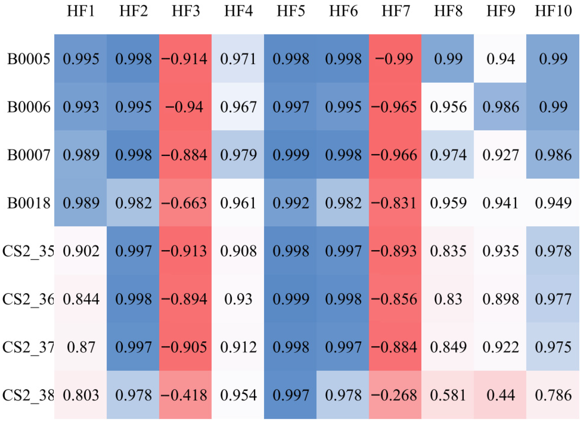
The resulting correlation heatmap is presented in Figure 3. As it shows, the deeper the red color in the graph, the closer its Pearson correlation coefficient is to -1, indicating a higher degree of negative correlation. The deeper the blue color, the closer its Pearson correlation coefficient is to 1, indicating a higher degree of positive correlation. An analysis of the correlation heatmap revealed that certain features exhibited strong correlations with the SOH in specific datasets but relatively weak correlations in others. Based on this observation, the feature selection principle adopted in this study requires that a feature must consistently demonstrate a high correlation with the SOH across all datasets. Features that display a high correlation in some datasets but a low correlation in others were excluded from the model inputs to ensure generalizability and robustness. As a result, these features were excluded from the final feature set. Following a comprehensive analysis, four features with the highest and most consistent correlations across both the NASA and CALCE datasets were selected as model input variables: HF2 (constant current charging time), HF4 (constant voltage discharging time between 4.0 V and 3.9 V), HF5 (current–time integral during charging), and HF6 (current–time integral during constant current charging). These features demonstrated robust and stable correlations with the battery SOH and were thus chosen as inputs for the proposed model.

2.3. Data Augmentation

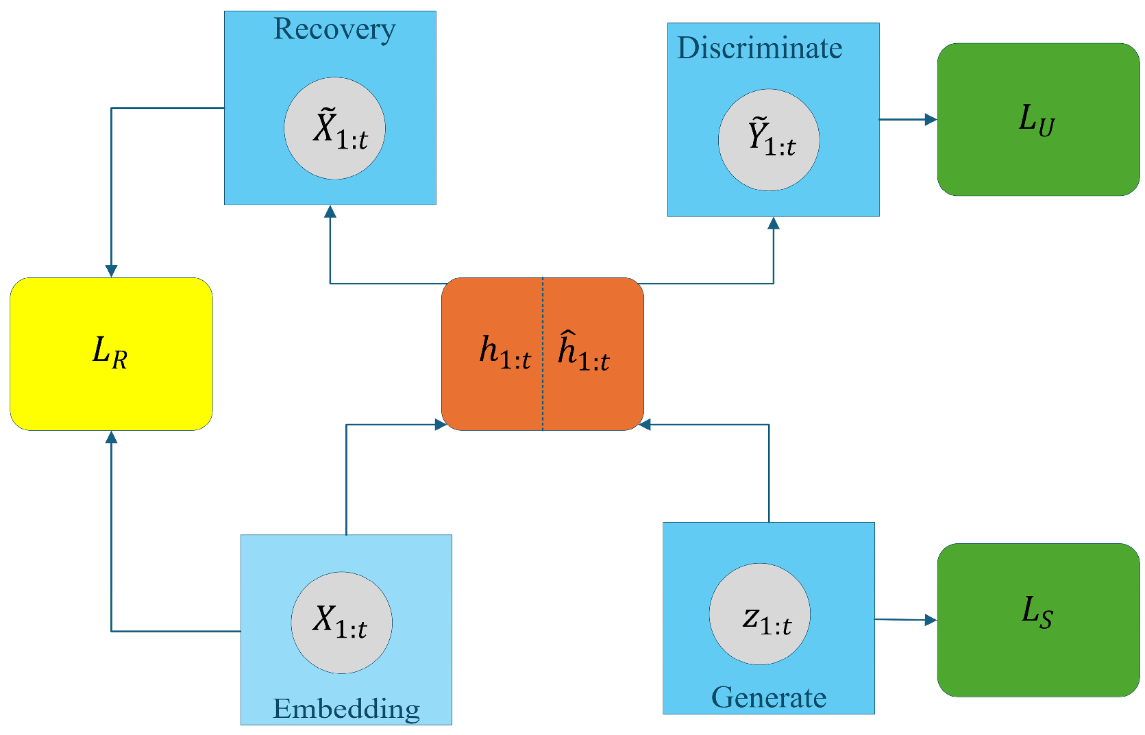
TimeGAN constitutes a deep-learning-based generative framework that is explicitly developed for the purpose of generating synthetic time-series data, aiming to generate high-fidelity synthetic sequences that preserve the authentic temporal dependencies inherent in real data. TimeGAN comprises four core modules: Embedder, Generator, Discriminator, and Recovery. The Embedder maps the original time series into a low-dimensional latent space; the Generator creates synthetic latent representations; the Recovery module reconstructs these latent representations back into the original data space; and the Discriminator differentiates between real and generated samples. The overall architecture is depicted in Figure 4.

In the TimeGAN model, the Embedder maps the real data $X_{1:t}$ into a low-dimensional space as $h_{1:t}$. This process not only helps capture the temporal dependencies within the data but also reduces the computational complexity and provides discriminative features for the subsequent Generator and Discriminator modules. The Recovery module reconstructs the original data ${\tilde{X}}_{1:t}$ from the embedded low-dimensional representation $h_{1:t}$, validating the effectiveness of the embedding layer by ensuring that the low-dimensional space retains the complete information of the original data, thus preventing information loss. The Generator produces a sequence $z_{1:t}$ of the same dimensionality as the original data from random noise, which is then embedded into the low-dimensional space as ${\widehat{h}}_{1:t}$. The Discriminator operates in the low-dimensional space to distinguish whether a given sequence ${\tilde{Y}}_{1:t}$ is real or generated. Real sequences are classified as 1, while generated sequences are classified as 0. Through adversarial training, the Generator is encouraged to produce increasingly realistic data that closely approximates the real data distribution.

During training, TimeGAN incorporates three loss functions. Firstly, since the embedding and recovery functions form a reversible mapping between the real data and the low-dimensional space, it is essential to accurately reconstruct the original data $X_{1:t}$ from its low-dimensional embedding $h_{1:t}$. This ensures that the low-dimensional representation does not deviate from the original data features. Therefore, the $L2$ norm of the difference between the original data $X_{1:t}$ and the reconstructed data ${\tilde{X}}_{1:t}$ after embedding and recovery is used as the first loss function, denoted as $L_R$; the formula is as follows:

$$L_R=E_{X_{1:t}~p}\left[{\displaystyle \sum _t{‖X_{1:t}-{\tilde{X}}_{1:t}‖}_2}\right]$$

(3)

where $E_{X_{1:t}\sim p}[·]$ denotes the expectation of the distribution of the time series with the real data distributed as $p$, and $\parallel ·{\parallel }_2$ is the $L2$ norm, which is used to measure the difference of the two sequences at each time step. The second loss function is the unsupervised adversarial loss, denoted as $L_U$; the formula is as follows:

$$L_U=E_{X_{1:t}~p}\left[{\displaystyle \sum _t\log y_t}\right]+E_{X_{1:t}~\widehat{p}}\left[{\displaystyle \sum _t\log (1-{\tilde{y}}_t)}\right]$$

(4)

where $\widehat{p}$ denotes the probability distribution of the generated data; the sequences $y_t$ and ${\tilde{y}}_t$ represent the Discriminator’s outputs for real and generated data, respectively.

Similar to the loss in traditional GANs, $L_U$ can be seen as an extension of the conventional GAN loss, but it operates in the latent low-dimensional space rather than the original data space. This approach significantly improves the computational efficiency and reduces the complexity. The discriminator evaluates the generated data, producing an output closer to 1 when the data closely resembles the real distribution, and closer to 0 when it deviates from the true values. Therefore, there is a third loss function. The third loss function is the supervised loss, denoted as $L_S$; the formula is as follows:

$$L_S=E_{X_{1:t}~p}\left[{\displaystyle \sum _t{‖h_{1:t}-g_x(h_{1:(t-1)},z_t)‖}_2}\right]$$

(5)

where $g_x(h_{1:(t-1)},z_t)$ denotes the next moment’s low-latitude vector predicted by the generator based on the previous moment’s low-latitude vector $h_{1:(t-1)}$, and the random noise $z_t$.

This design forces the generator to match the original data’s temporal patterns by comparing the outputs with real samples at each time step, facilitating the learning of complex feature dynamics. The generator $g_x(h_{t-1},z_t)$ produces a value by taking the embedded data $h_{t-1}$ from the previous time step and a new random noise $z_t$. This generated sequence is then compared with the embedded original sequence $h_{1:t}$. The total loss function $L$ is optimized during training by simultaneously optimizing the embedding network ${\theta }_e$, the recovery network ${\theta }_r$, the generator ${\theta }_g$ and the discriminator ${\theta }_d$ and combining the three loss functions mentioned above using the following optimization function:

$$L=\underset{{\theta }_e,{\theta }_r}{\min }(\lambda L_S+L_R)+\underset{{\theta }_g}{\min }(\eta L_S+\underset{{\theta }_d}{\max }{L}_U)$$

(6)

where $\lambda$ and $\eta$ are hyperparameters to balance the weights of different losses.

This approach enables the generated data to capture not only the temporal features within each sequence but also the interrelationships among multiple features, while ensuring that the synthetic sequences exhibit dynamic characteristics consistent with the real data at local time steps. Consequently, TimeGAN effectively models complex temporal dynamics, which has contributed to its widespread adoption across diverse application domains. Four battery specimens from the NASA database were adopted as the primary data origin for the present study. TimeGAN is employed for data augmentation, generating multiple augmented datasets to train subsequent models.

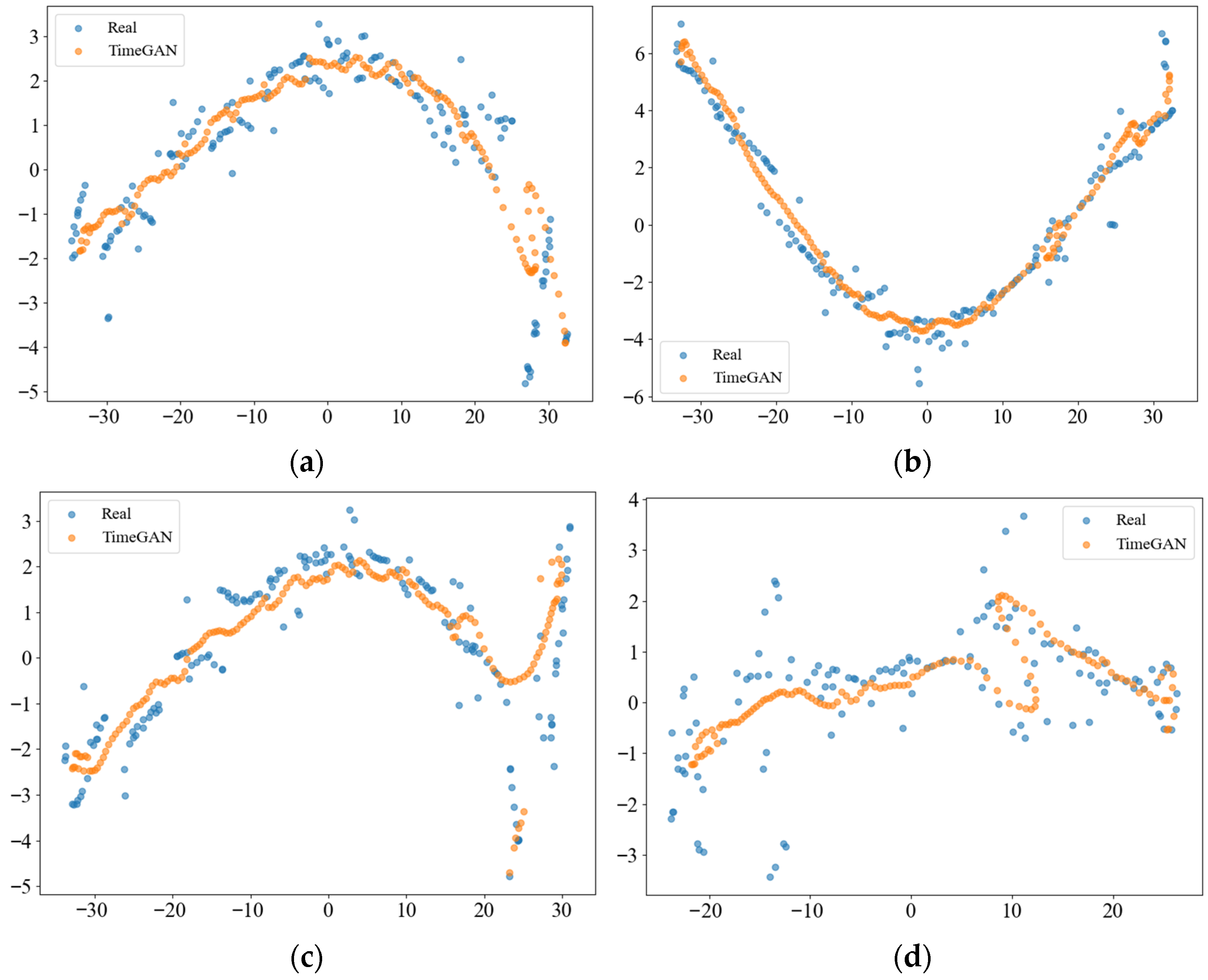
To further evaluate the consistency between real and synthetic datasets, the t-distributed stochastic neighbor embedding (t-SNE) technique was adopted to reduce the high-dimensional feature space to a two-dimensional manifold for graphical interpretation. By preserving local neighborhood structures, t-SNE enables an intuitive comparison of the intrinsic structural features between real and generated samples. Figure 5 presents the t-SNE analysis plots for each dataset and the generated data. The plots reveal that the overall distributions of the generated data closely resemble those of the real data, indicating that the generated data preserves local structural features similar to the original dataset. Additionally, the mean and standard deviation for each feature across both datasets were calculated, as shown in the formula below:

$$\mu ={\displaystyle \frac{1}{n}}{\displaystyle {\sum }_{i=1}^n{X}_i}$$

(7)

$$\sigma =\sqrt{{\displaystyle \frac{1}{n-1}}{\displaystyle {\sum }_{i=1}^n{(X_i-\mu )}^2}}$$

(8)

where $\mu$ represents the mean and $\sigma$ represents the standard deviation.

The mean and standard deviation for each feature are listed in

Table 4. Mean and standard deviation of the original features.

Dataset		HF2	HF4	HF5	HF6	SOH
B0005	Mean	2405.2	91.4	5691.9	3618.3	0.787
	Standard deviation	595.2	35.5	706.2	899.5	0.094
B0006	Mean	2101.2	49.6	5628.1	3164.8	0.775
	Standard deviation	813.5	40.8	918.3	1231.2	0.124
B0007	Mean	2681.1	113.4	5994.4	3986.1	0.821
	Standard deviation	473.7	34.1	584.4	706.3	0.08
B0018	Mean	2424.7	672.8	5690.9	3638.5	0.78
	Standard deviation	425.6	125.9	545.6	654.3	0.076

and

Table 5. Mean and standard deviation of generated features.

Dataset		HF2	HF4	HF5	HF6	SOH
B0005	Mean	2403.1	91.4	5688.9	3615.3	0.787
	Standard deviation	595.2	35.5	698.6	889.5	0.093
B0006	Mean	2099.3	49.6	5625.6	3162	0.775
	Standard deviation	808.4	40	911.2	1224	0.123
B0007	Mean	2674.1	112.8	5985.5	3975.2	0.822
	Standard deviation	473.8	33.7	583.6	705.7	0.079
B0018	Mean	2425.7	673.9	5694.1	3644.2	0.781
	Standard deviation	412.3	124.8	539.6	638.3	0.075

. For most features, the relative differences between the corresponding statistical moments remain small, indicating that the synthetic data maintains consistency in the first- and second-order statistical properties. In summary, the comprehensive results demonstrate that the synthetic dataset possesses distribution characteristics comparable to the real dataset. It exhibits statistical consistency for data augmentation in SOH estimation models and can serve as supplementary data for model inputs.

3. Model Architecture

3.1. LSTM Network

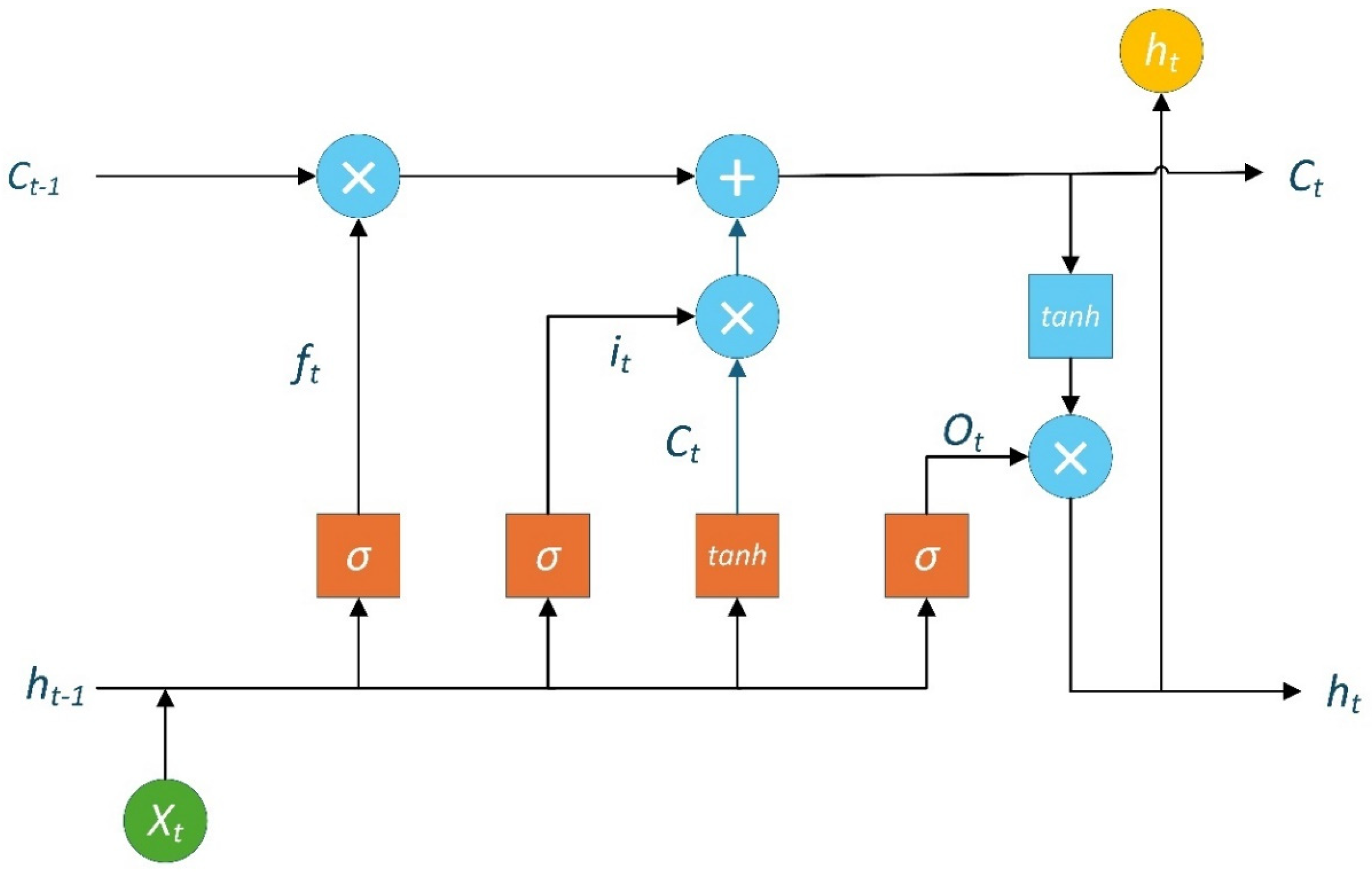
LSTM is a specialized variant of the RNN, whose structure is shown in Figure 5 [32]. The fundamental advancement of the LSTM network is its memory-augmented architecture, centered on a cell state that enables information retention across long sequences. This capability is governed by a gating system comprising three specialized units—the forget, input, and output gates—which collectively manage the flow of information into and out of the memory cell. The cell state is propagated linearly through time steps, effectively alleviating the problem of gradient vanishing during backpropagation. Specifically, the forget gate controls the extent to which previous cell state information is retained, the input gate governs the incorporation of new information into the cell state, and the output gate determines the information to be exposed as the hidden state at the current time step. This architectural design enables LSTM networks to effectively capture short-term dynamic variations while preserving long-term dependency features, which has led to their extensive adoption across various fields including sequential data analysis, acoustic signal processing, and computational linguistics. The structure of the LSTM is illustrated in Figure 6, and the detailed calculation process is as follows: given an input sequence ${\left\{X_t\right\}}_{t=1}^T$, the hidden state $h_t$ and cell state $C_t$ at time step $t$ are updated through the following gating functions:

$$f_t=\sigma (W_f\cdot \left[h_{t-1},x_t\right]+b_f)$$

(9)

$$i_t=\sigma (W_i\cdot \left[h_{t-1},x_t\right]+b_i)$$

(10)

$$\widetilde{C_t}=\tanh (W_C\cdot \left[h_{t-1},x_t\right]+b_c)$$

(11)

$$C_t=f_t\cdot C_{t-1}+i\widetilde{C_t}$$

(12)

$$o_t=\sigma (W_o\cdot \left[h_{t-1},x_t\right]+b_o)$$

(13)

$$h_t=o_t\tanh (C_t)$$

(14)

where $\sigma$ is the Sigmoid function pressing the output into the [0, 1] interval; $f_t$ denotes the forget gate; $i_t$ represents the input gate; $\widetilde{C_t}$ is the candidate cell state; $C_t$ is the updated cell state; $o_t$ indicates the output gate; and $h_t$ is the hidden state. The matrices $W_i$, $W_f$, $W_o$, and $W_c$ correspond to the weight parameters for the input gate, forget gate, output gate, and candidate cell state, respectively. Similarly, $b_i$, $b_f$, $b_o$, and $b_c$ are the associated bias vectors for each respective gate and the candidate cell state update.

3.2. iTransformer

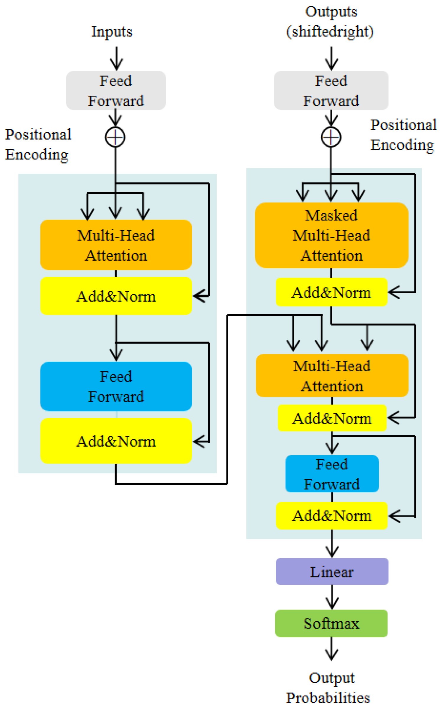
The Transformer model is a deep neural network architecture built entirely upon the attention mechanism, as shown in Figure 7 [33,34]. Unlike the traditional RNN and CNN, the Transformer removes the constraints of sequential computation and limited receptive fields. Instead, it employs a self-attention mechanism to directly capture the global dependencies among all positions within an input sequence, thereby greatly improving the modeling efficiency and enabling a fully parallel computation. The overall architecture follows the classic encoder–decoder framework. Each encoder layer contains two primary sublayers: (1) a multi-head self-attention module and (2) a position-wise feedforward neural network. Both sublayers incorporate residual connections and layer normalization to stabilize the training and accelerate the convergence. At the core of the self-attention mechanism lies the process of mapping the input sequence into vectors—query ($Q\in R^{n\times d_k}$), key ($K\in R^{n\times d_k}$), and value ($V\in R^{n\times d_v}$)—where $n$ is the sequence length, $d_k$ is the dimensionality of queries and keys, and $d_v$ is the dimensionality of values.

Attention weights are computed by measuring the similarity between queries and keys, which are then used to dynamically weight the values, enabling the model to selectively focus on relevant features and effectively reconstruct the input representation. The self-attention mechanism is calculated as follows:

$$Attention(Q,K,V)=softmax({\displaystyle \frac{Q{K}^T}{\sqrt{d_k}}})V$$

(15)

where the scaling factor $\sqrt{d_k}$ is used to counteract the potential for large dot-product magnitudes, which can lead to small gradients and hinder effective learning. The corresponding calculation results are processed using the softmax function to obtain the final value. Multi-head attention is realized by executing multiple independent self-attention computations in parallel, which are formulated as follows:

$$hea{d}_i=Attention(Q{W}_i^Q,K{W}_i^K,Q{W}_i^V)$$

(16)

where $W_i^Q\in R^{d_{model}\times d_k}$, $W_i^K\in R^{d_{model}\times d_k}$, and $W_i^V\in R^{d_{model}\times d_v}$.

The multi-head attention mechanism concatenates the outputs of all heads and projects them back to the model dimension, as expressed in the following equation:

$$MultiHead(Q,K,V)=Concat(hea{d}_1, \dots ,hea{d}_h)W^O$$

(17)

where ${\mathrm{W}}^O\in R^{h·d_v\times d_{model}}$, which significantly enhances the model’s ability to capture information from different semantic subspaces. To compensate for the lack of sequence order information, the Transformer introduces positional encoding. This is implemented by injecting position-dependent signals using sinusoidal functions, enabling the model to perceive relative positions of elements without relying on recurrence. This design overcomes the sequential computation bottleneck inherent in RNNs, allowing the fully parallel processing of sequence data and significantly improving the training efficiency.

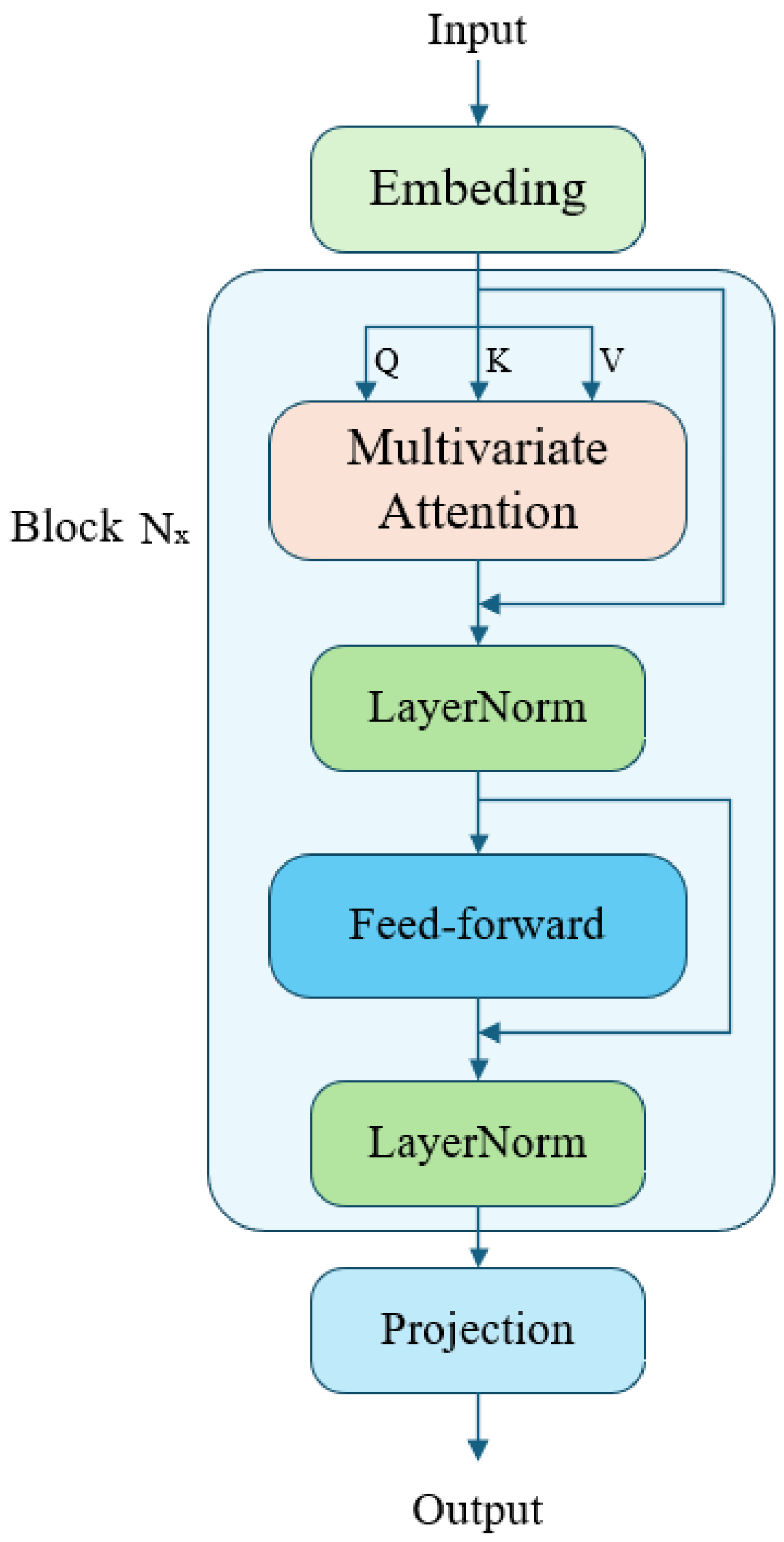
The iTransformer adopted in this paper is an improved Transformer architecture specifically tailored for time-series forecasting tasks, with its overall structure illustrated in Figure 7. Compared to the standard Transformer model, the iTransformer retains only the encoder components—comprising the embedding layer, encoder blocks, and projection layer—as its core modules. Unlike the conventional Transformer, which uniformly processes the entire time series, the iTransformer emphasizes the heterogeneity among multiple variables in its architectural design. As depicted in Figure 8, the iTransformer first maps each time series into variable-specific representations via dedicated variable token embeddings, thereby preserving the unique semantic attributes of each variable. Subsequently, the model encodes different variables as separate temporal sequences, with positional encoding implemented through feedforward networks. Building on this, the self-attention mechanism computes attention weights across variables, effectively modeling the dependencies and latent co-evolutionary patterns among them. A key innovation of the iTransformer lies in its “variable separation modeling” strategy. Rather than embedding all variables into a single unified sequence, the iTransformer independently models the dynamic features of each variable while adaptively assigning higher attention weights to strongly correlated variables. This design significantly enhances the model’s capacity to capture complex multivariate relationships and evolving temporal trends, rendering it particularly well-suited for multivariate time-series forecasting tasks.

3.3. Data Flow Direction

The overall data flow of the TimeGAN-based LSTM-iTransformer model is illustrated in Figure 9. First, ten relevant features are extracted from the raw battery data. A correlation analysis is performed to select the four most correlated features as the initial feature set. This initial feature set is then fed into TimeGAN to generate a corresponding synthetic feature set. Both the synthetic and initial feature sets are subsequently input into the LSTM model for local feature extraction. After LSTM preprocessing, the features are further input into the iTransformer model for global modeling. Following multiple training iterations, the model outputs the SOH estimation value.

4. Experimental Results

To comprehensively evaluate the performance of the proposed model, a series of experiments were conducted comparing it with several widely used deep-learning algorithms. The model performance is assessed using three metrics: Root Mean Square Error (RMSE), Mean Absolute Error (MAE), and Mean Absolute Percentage Error (MAPE). The corresponding calculation formulae are presented below:

$$RMSE=\sqrt{{\displaystyle \frac{{\displaystyle {\sum }_{i=1}^N(SO{H}_i-\widehat{SO{H}_i})}}{N}}}$$

(18)

$$MAE={\displaystyle \frac{1}{N}}{\displaystyle {\sum }_{i=1}^N\left|SO{H}_i-\widehat{SO{H}_i}\right|}$$

(19)

$$MAPE={\displaystyle \frac{1}{N}}{\displaystyle {\sum }_{i=1}^N\left|\frac{SO{H}_i-\widehat{SO{H}_i}}{\widehat{SO{H}_i}}\right|}\times 100\%$$

(20)

where $S\widehat{O}{H}_i$ is the predicted value of the model and ${SOH}_i$ is the true value.

In this section, Section 4.1 validates the effectiveness of the data augmentation technique. Section 4.2 conducts experiments using the extended aging sample set and compares the performance of the proposed model with the rest of the common models.

Section 4.3 further compares the performance of the target model on the CALCE dataset.

Table 6. Hyperparameters employed by the model during the experiment.

Category	Parameter	Value
Input Setting	Input sequence length	9
	Prediction length	1
	Input feature dimension	4
LSTM	Hidden size	64
	Number of layers	1
	Bidirectional	NO
	Dropout	0.1
iTransformer	Embedding dimension	128
	Number of attention heads	8
	Encoder layers	1
	Feedforward dimension	64
	Attention factor	5
	Activation function	GELU
Training Setting	Optimizer	Adam
	Batch size	128
	Epochs	300
	Loss function	MSE
	Early stopping ratio	0.2
	Random seed	43

presents the specific hyperparameters of the model during the experiment.

4.1. Comparison Experiments Before and After Data Augmentation

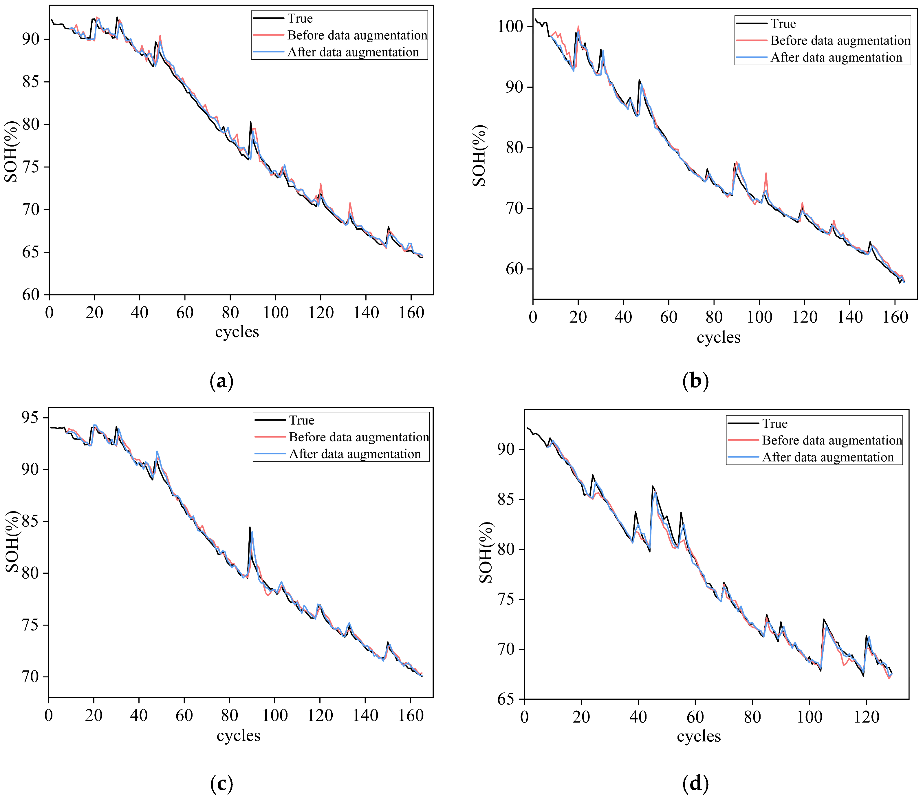
To validate the effectiveness of the proposed data augmentation technique, two groups of comparative experiments were designed based on the LSTM-iTransformer model. The control group was trained and tested using the original data without augmentation. The specific training strategy is as follows: when using the B0005 dataset as the test set, the remaining three datasets (B0006, B0007, and B0018) are used as the training set; similarly, when selecting any one of B0006, B0007, or B0018 as the test set, the other three original datasets were used for training. The experimental group employed the augmented expanded dataset generated through data augmentation, with training and testing strategies consistent with the control group. Figure 10 illustrates the estimation curves of the model in both experimental groups. The results indicate that, compared to the control group, the model trained on the augmented data produces estimation curves closer to the true SOH values, demonstrating a stronger capability in capturing aging trends. Furthermore, the proposed approach demonstrates an enhanced capability in capturing capacity regeneration dynamics, leading to more precise and dependable SOH predictions. The RMSE, MAE, and MAPE of the model for each test set are also presented in

Table 7. Comparison of metrics before and after data augmentation.

Dataset		Before	After
	RMSE(%)	0.5565	0.4084
B0005	MAE(%)	0.3516	0.2871
	MAPE(%)	0.4451	0.3643
	RMSE(%)	1.0131	0.8638
B0006	MAE(%)	0.5945	0.4705
	MAPE(%)	0.7409	0.5958
	RMSE(%)	0.5695	0.5447
B0007	MAE(%)	0.3656	0.3416
	MAPE(%)	0.4420	0.4125
	RMSE(%)	0.6573	0.5917
B0018	MAE(%)	0.4437	0.3855
	MAPE(%)	0.5689	0.4976

, from which it can be seen. on the B0005 dataset, that the RMSE, MAE, and MAPE are boosted by 27%, 18%, and 18%, while, for the B0006 dataset, the RMSE, MAE, and MAPE were boosted by 15%, 21%, and 20%, respectively, while, for the B0007 dataset, it was improved by 4%, 6.5%, and 6.7%, respectively. The effect for the B0018 dataset was improved by 10%, 13.1%, and 12.5%, respectively. The increased training data enhanced the model’s estimation performance, effectively addressing the issue of insufficient training samples. By augmenting the original data to generate new training samples, both the quantity and diversity of the data are expanded, which improves the training performance of the model. It enabled the model to better capture the aging characteristics of the battery and significantly improves its predictive performance.

4.2. Model Comparison

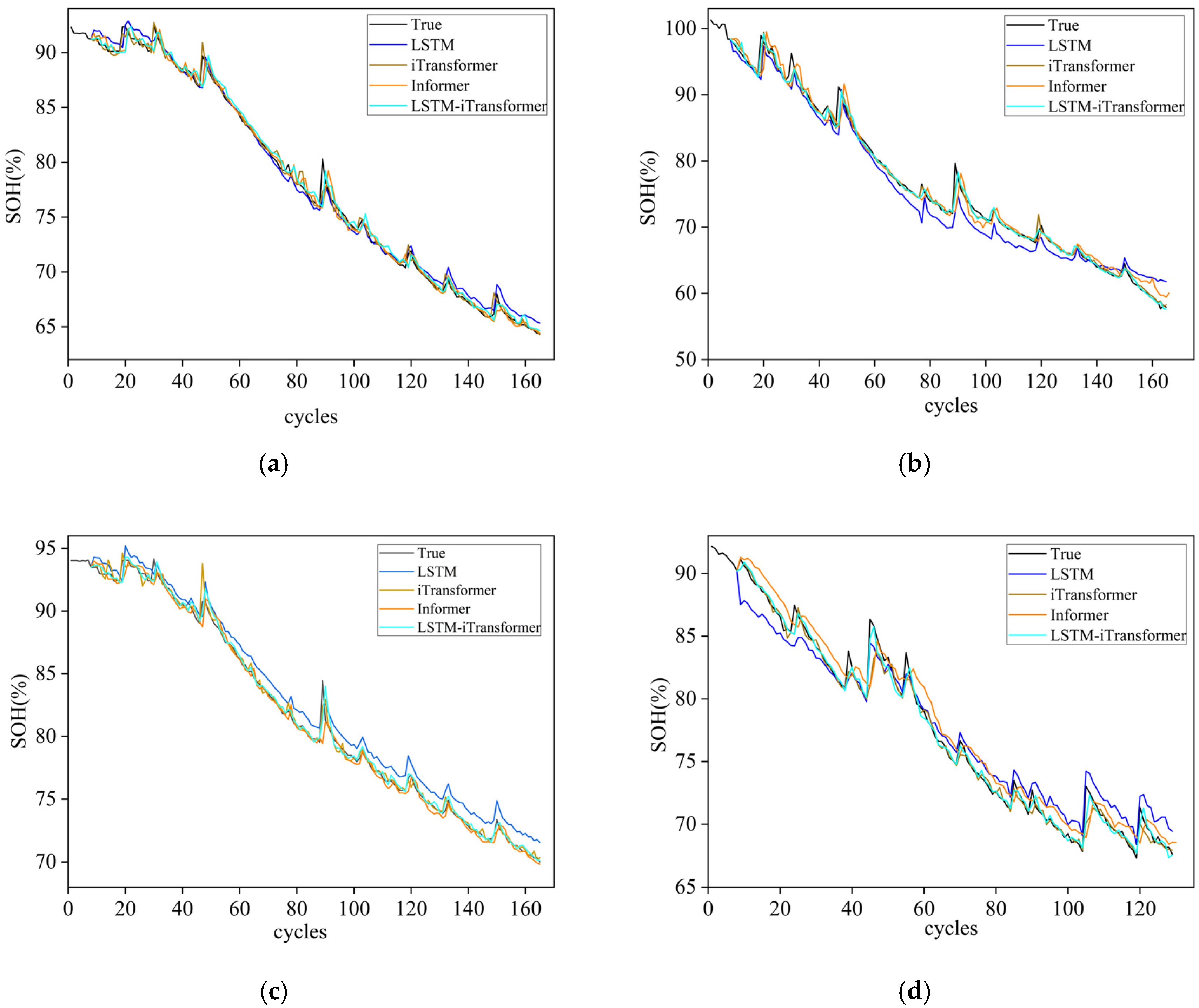
To further validate the effectiveness of the proposed LSTM-iTransformer model, this section compares its performance against several commonly used deep-learning models, including LSTM, Informer, and iTransformer. All experiments in this section are performed on augmented data after augmentation using TimeGAN on B0005, B0006, B0007, and B0018 data. The training sets comprise augmented data from three batteries excluding the one used for testing, while the test sets consist of the original data of the corresponding test battery. Figure 11 presents the estimation curves of each model. The comparison chart, which includes six predicted curves alongside the true values, reveals that several models gradually lose the ability to accurately capture battery aging information during the later stages of the estimation horizon. In contrast, the LSTM-iTransformer model consistently maintains a strong capability in tracking the battery aging trend, particularly in the later estimation periods. The close correspondence between the model outputs and experimental results validates its superior tracking performance.

Table 8. Comparison of experimental metrics on the NASA dataset.

Dataset		LSTM	Informer	iTransformer	LSTM- iTransformer
	RMSE(%)	0.7358	0.5247	0.4822	0.4084
B0005	MAE(%)	0.5546	0.3484	0.3125	0.2871
	MAPE(%)	0.7282	0.4426	0.3999	0.3643
	RMSE(%)	2.0422	1.1004	1.0825	0.8638
B0006	MAE(%)	1.6149	0.7618	0.5925	0.4705
	MAPE(%)	2.2031	1.009	0.7343	0.6037
	RMSE(%)	1.0982	0.5710	0.5268	0.5447
B0007	MAE(%)	1.0556	0.4035	0.3312	0.3416
	MAPE(%)	1.3247	0.4951	0.3915	0.4125
	RMSE(%)	1.4204	0.9730	0.7985	0.5917
B0018	MAE(%)	1.2346	0.8214	0.4763	0.3855
	MAPE(%)	1.6229	1.0648	0.6071	0.4976

summarizes the evaluation metrics for each model, including the RMSE, MAE, and MAPE. The LSTM-iTransformer’s RMSE fluctuates between 0.408% and 0.863%, MAE between 0.287% and 0.47%, and MAPE between 0.364% and 0.603%. The iTransformer model achieves RMSE, MAE, and MAPE ranges of 0.482–1.08%, 0.312–0.592%, and 0.399–0.734%, respectively. iTransformer attains the best test metrics on the B0007 dataset. That is because the noise from battery B0007 is relatively small, and modeling iTransformer alone is sufficient. The advantage of “local smoothing preprocessing” in LSTM is not obvious. But the performance gap between LSTM-iTransformer and iTransformer remains marginal and acceptable. LSTM’s performance lies within 0.735–2.04% (RMSE), 0.554–1.61% (MAE), and 0.728–2.203% (MAPE). The performance of Informer ranges from 0.52% to 1.1% (RMSE), 0.34% to 0.82% (MAE), and 0.44% to 1.06% (MAPE) respectively. Overall, the LSTM-iTransformer model significantly outperforms the LSTM and Informer models. Moreover, the introduction of the LSTM module further enhances performance compared to the iTransformer, indicating the positive contribution of LSTM in boosting model accuracy. In summary, both the metric analysis and the estimation curve demonstrate that iTransformer outperforms the LSTM and Informer models, while the LSTM-iTransformer model achieves a better predictive accuracy than iTransformer.

4.3. Experiments on CALCE

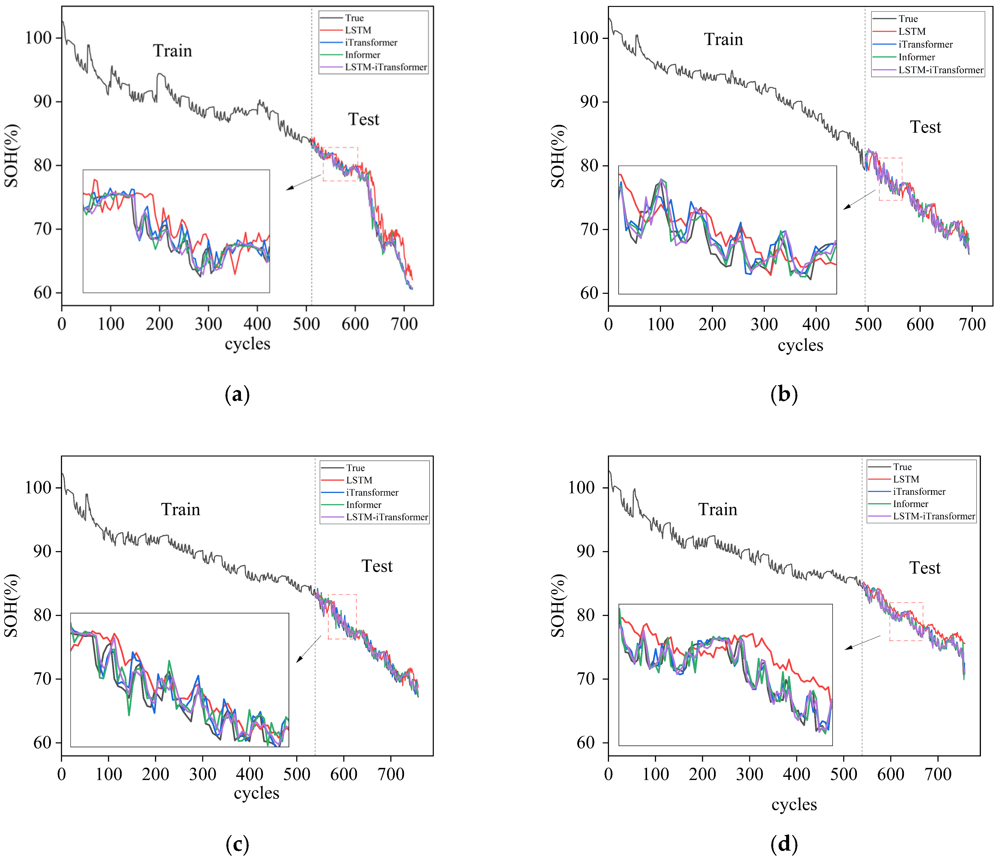
To further evaluate the generalization capability of the proposed model, experiments were conducted on the CALCE dataset. Compared to the NASA dataset, the CALCE dataset, provided by the University of Maryland, contains a richer collection of battery aging data. Owing to the larger scale of the dataset, data augmentation is not applied to enlarge the sample space. To strictly avoid temporal information leakage in time-series forecasting, the CALCE dataset was divided in chronological order rather than randomly. Specifically, the first 70% of battery cycles were used for training, while the remaining 30% of later cycles were reserved for testing. Therefore, the model was trained only on historical data and evaluated on future unseen cycles. The estimation results, compared against the LSTM, Informer, and iTransformer models, are shown in Figure 12. It can be observed that, compared to the NASA dataset, the CALCE dataset exhibits higher noise levels and more pronounced capacity regeneration phenomena. Compared to other models, this method demonstrates a superior trajectory consistency within the regeneration region and can reproduce local rebound trends, indicating its stable modeling capability even under regeneration-induced fluctuating conditions.

Table 9. Comparison of test metrics on the CALCE dataset.

Dataset		LSTM	Informer	iTransformer	LSTM- iTransformer
	RMSE(%)	1.2446	0.6024	0.6845	0.5132
CS2_35	MAE(%)	0.9201	0.3860	0.4581	0.3552
	MAPE(%)	1.3132	0.5326	0.6283	0.4845
	RMSE(%)	1.0016	0.7456	0.7506	0.7185
CS2_36	MAE(%)	0.8237	0.5270	0.5318	0.5309
	MAPE(%)	1.1077	0.7289	0.7235	0.7211
	RMSE(%)	0.8341	0.6111	0.6148	0.5759
CS2_37	MAE(%)	0.7066	0.4551	0.4541	0.4322
	MAPE(%)	0.9449	0.6054	0.6057	0.5753
	RMSE(%)	1.1254	0.6398	0.6168	0.5332
CS2_38	MAE(%)	0.9103	0.6398	0.4082	0.3673
	MAPE(%)	1.1783	0.5287	0.5231	0.4707

presents the test performance metrics of each model. From the values listed in the table, it can be seen that LSTM-iTransformer has the best performance on all four datasets. Based on the above analysis, it can be concluded that the LSTM-iTransformer model outperforms LSTM, Informer, and iTransformer in estimation accuracy. Moreover, compared with the iTransformer, the LSTM iTransformer combined with the LSTM module delivers a significant improvement in system performance. In summary, LSTM iTransformer has demonstrated a strong predictive ability in SOH estimation.

4.4. Computational Efficiency Analysis

In this section, the training cost and computational resource consumption of different models are further investigated.

Table 10. Computational efficiency of different models across various datasets.

Dataset	LSTM	Informer	LSTM- iTransformer
B0005	17.74 s	65.77 s	49.50 s
B0006	17.66 s	65.78 s	51.67 s
B0007	18.06 s	65.79 s	52.52 s
B0018	18.91 s	66.73 s	50.51 s
CS2_35	10.19 s	57.41 s	28.46 s
CS2_36	10.08 s	71.51 s	32.62 s
CS2_37	11.23 s	65.36 s	23.58 s
CS2_38	11.12 s	63.96 s	31.27 s

presents the training time of the LSTM, Informer, and the proposed LSTM-iTransformer models under identical hyperparameter settings and the same training dataset scale. To ensure fairness and stability, each experiment was repeated five times, and the average value was reported. As shown in the table, the LSTM model exhibits the shortest training time, which reflects its relatively simple architecture and lower computational complexity. Consequently, it requires fewer computational resources during training. In contrast, the Informer model shows the longest training time, indicating its more complex structure and the additional computational overhead introduced by the self-attention mechanism. The proposed LSTM-iTransformer model ranks between the two baseline models in terms of the training time. Although its training cost is higher than that of the conventional LSTM model, the experimental results presented in the previous sections demonstrate a significant improvement in SOH estimation accuracy. Meanwhile, despite the higher computational cost of the Informer model, its estimation accuracy remains inferior to that of the proposed model. These results indicate that the proposed LSTM-iTransformer achieves an improved estimation performance with a moderate increase in computational complexity. Therefore, it effectively balances the prediction accuracy and computational efficiency, highlighting its potential applicability in practical Battery Management System (BMS) scenarios.

5. Conclusions

This paper proposes an innovative method for estimating the battery SOH. Initially, multiple indicators closely related to battery aging were extracted from the charge–discharge curves and IC curves. A Pearson correlation analysis was employed to select features exhibiting a strong correlation with the SOH, which served as inputs for the model. To address the insufficient battery aging data, a time-series data augmentation technique based on TimeGAN was designed and introduced. It effectively expands the number of aging samples and alleviates the limitations posed by insufficient training data, especially for SOH estimation that heavily relies on large datasets. Moreover, this study presents a hybrid model combining LSTM networks and an improved Transformer architecture (LSTM-iTransformer). The LSTM component excels at capturing both long- and short-term temporal dependencies during feature preprocessing, while the iTransformer employs a powerful self-attention mechanism to accurately model global temporal dependencies and complex multivariate relationships. Combining the advantages of both provides an efficient and accurate framework for battery SOH estimation. By leveraging publicly available datasets from NASA and CALCE for experimental validation, the results demonstrate that the proposed method markedly improves both the accuracy of SOH estimation and its generalization capability, indicating strong prospects for practical application. Nevertheless, the research has not fully considered batteries with a broader range of battery chemistries. Consequently, the generalizability of the proposed methodology remains to be further substantiated. Future work will focus on expanding the data collection and experimental testing across diverse battery chemistries, with an emphasis on investigating multifactorial aging characteristics. This will enhance the model’s applicability and predictive accuracy across a broader range of scenarios, thereby offering robust technical support for a precise battery health assessment.

References

1. Linghu, J.Q.; Kang, L.Y.; Liu, M.; Luo, X.; Feng, Y.B.; Lu, C.S. Estimation for state-of-charge of lithium-ion battery based on an adaptive high-degree cubature Kalman filter. Energy 2019, 189, 116204. [Google Scholar] [CrossRef] [Scilit]
2. Li, X.Y.; Xu, J.H.; Hong, J.X.; Tian, J.D.; Tian, Y. State of energy estimation for a series-connected lithium-ion battery pack based on an adaptive weighted strategy. Energy 2021, 214, 118858. [Google Scholar] [CrossRef] [Scilit]
3. Linghu, J.; Kang, L.; Liu, M.; Hu, B.; Wang, Z. An Improved Model Equation Based on a Gaussian Function Trinomial for State of Charge Estimation of Lithium-ion Batteries. Energies 2019, 12, 1366. [Google Scholar] [CrossRef] [Scilit]
4. Wu, J.; Fang, L.C.; Dong, G.Z.; Lin, M.Q. State of health estimation of lithium-ion battery with improved radial basis function neural network. Energy 2023, 262, 125380. [Google Scholar] [CrossRef] [Scilit]
5. Jia, C.; Liu, W.; He, H.; Chau, K.T. Health-conscious energy management for fuel cell vehicles: An integrated thermal management strategy for cabin and energy source systems. Energy 2025, 333, 137330. [Google Scholar] [CrossRef] [Scilit]
6. Zhou, J.; Rong, J.; Zhang, J.; Liu, C.; Yi, F.; Jiao, Z.; Zhang, C. Deep learning estimation of state of health for lithium-ion batteries using multi-level fusion features of discharge curves. J. Power Sources 2025, 653, 237781. [Google Scholar] [CrossRef] [Scilit]
7. Hussain, A.; Mehmood, A.; Raza, W.; Faheem, M.; Saleem, A.; Kashif Majeed, M.; Iqbal, R.; Aziz, M.A. Highly Stretchable Polyurethane Porous Membranes with Adjustable Morphology for Advanced Lithium Metal Batteries. Chem. Asian J. 2024, 19, e202400245. [Google Scholar] [CrossRef] [Scilit]
8. Zeng, C.; Xu, C.; Li, H.; Wang, K. A novel ensemble learning model for state of health estimation of lithium-ion batteries. J. Power Sources 2025, 638, 236608. [Google Scholar] [CrossRef] [Scilit]
9. Saleem, A.; Iqbal, R.; Majeed, M.K.; Hussain, A.; Akbar, A.R.; Hussain, Z.; Jabar, B.; Rauf, S.; Shaw, L.L. Boosting lithium-ion conductivity of polymer electrolyte by selective introduction of covalent organic frameworks for safe lithium metal batteries. Nano Energy 2024, 128, 109848. [Google Scholar] [CrossRef] [Scilit]
10. Tian, A.; Dong, K.; Yang, X.-G.; Wang, Y.; He, L.; Gao, Y.; Jiang, J. Physics-based parameter identification of an electrochemical model for lithium-ion batteries with two-population optimization method. Appl. Energy 2025, 378, 124748. [Google Scholar] [CrossRef] [Scilit]
11. Jia, C.; Liu, W.; Chau, K.T.; He, H.; Zhou, J.; Niu, S. Passenger-aware reinforcement learning for efficient and robust energy management of fuel cell buses. eTransportation 2026, 27, 100537. [Google Scholar] [CrossRef] [Scilit]
12. Liu, X.; Yang, K.; Zou, B.; Zhang, X.; Bao, G.; Ma, B.; Zhang, L.; Tan, R. Accurate estimation of state of health for lithium-ion batteries based on Pyraformer and TimeGAN data augmentation. J. Power Sources 2025, 640, 236722. [Google Scholar] [CrossRef] [Scilit]
13. Acquarone, M.; Miretti, F.; Giuliacci, T.A.; Duque, J.; Misul, D.A.; Kollmeyer, P. Regression based battery state of health estimation for multiple electric vehicle fast charging protocols. J. Power Sources 2024, 624, 235601. [Google Scholar] [CrossRef] [Scilit]
14. Shao, L.; Zhang, Y.; Zheng, X.; Yang, R.; Zhou, W. SOH estimation of lithium-ion batteries subject to partly missing data: A Kolmogorov–Arnold–Linformer model. Neurocomputing 2025, 638, 130181. [Google Scholar] [CrossRef] [Scilit]
15. Amiri, M.N.; Håkansson, A.; Burheim, O.S.; Lamb, J.J. Lithium-ion battery digitalization: Combining physics-based models and machine learning. Renew. Sustain. Energy Rev. 2024, 200, 114577. [Google Scholar] [CrossRef] [Scilit]
16. Tian, J.; Xu, R.; Wang, Y.; Chen, Z. Capacity attenuation mechanism modeling and health assessment of lithium-ion batteries. Energy 2021, 221, 119682. [Google Scholar] [CrossRef] [Scilit]
17. Locorotondo, E.; Cultrera, V.; Pugi, L.; Berzi, L.; Pierini, M.; Lutzemberger, G. Development of a battery real-time state of health diagnosis based on fast impedance measurements. J. Energy Storage 2021, 38, 102566. [Google Scholar] [CrossRef] [Scilit]
18. Demirci, O.; Taskin, S.; Schaltz, E.; Acar Demirci, B. Review of battery state estimation methods for electric vehicles-Part II: SOH estimation. J. Energy Storage 2024, 96, 112703. [Google Scholar] [CrossRef] [Scilit]
19. Vignesh, S.; Che, H.S.; Selvaraj, J.; Tey, K.S.; Lee, J.W.; Shareef, H.; Errouissi, R. State of Health (SoH) estimation methods for second life lithium-ion battery—Review and challenges. Appl. Energy 2024, 369, 123542. [Google Scholar] [CrossRef] [Scilit]
20. Ouyang, T.; Su, Y.; Wang, C.; Jin, S. Combined Meta-Learning With CNN-LSTM Algorithms for State-of-Health Estimation of Lithium-Ion Battery. IEEE Trans. Power Electron. 2024, 39, 10106–10117. [Google Scholar] [CrossRef] [Scilit]
21. Mo, D.; Wang, S.; Fan, Y.; Takyi-Aninakwa, P.; Zhang, M.; Wang, Y.; Fernandez, C. Enhanced multi-constraint dung beetle optimization-kernel extreme learning machine for lithium-ion battery state of health estimation with adaptive enhancement ability. Energy 2024, 307, 132723. [Google Scholar] [CrossRef] [Scilit]
22. Kurucan, M.; Özbaltan, M.; Yetgin, Z.; Alkaya, A. Applications of artificial neural network based battery management systems: A literature review. Renew. Sustain. Energy Rev. 2024, 192, 114262. [Google Scholar] [CrossRef] [Scilit]
23. Shrivastava, P.; Naidu, P.A.; Sharma, S.; Panigrahi, B.K.; Garg, A. Review on technological advancement of lithium-ion battery states estimation methods for electric vehicle applications. J. Energy Storage 2023, 64, 107159. [Google Scholar] [CrossRef] [Scilit]
24. Bodnár, D.; Ram Chandra Mouli, G.; Ďurovský, F.; Bauer, P.; Qin, Z. Semi-Empirical Model of Nickel Manganese Cobalt (NMC) Lithium-Ion Batteries Including Capacity Regeneration Phenomenon. IEEE Trans. Transp. Electrif. 2025, 11, 797–813. [Google Scholar] [CrossRef] [Scilit]
25. Sangiri, J.B.; Kulshreshtha, T.; Ghosh, S.; Maiti, S.; Chakraborty, C. A novel methodology to estimate the state-of-health and remaining-useful-life of a Li-ion battery using discrete Fourier transformation. J. Energy Storage 2022, 46, 103849. [Google Scholar] [CrossRef] [Scilit]
26. Ma, L.; Xu, Y.; Zhang, H.; Yang, F.; Wang, X.; Li, C. Co-estimation of state of charge and state of health for lithium-ion batteries based on fractional-order model with multi-innovations unscented Kalman filter method. J. Energy Storage 2022, 52, 104904. [Google Scholar] [CrossRef] [Scilit]
27. Guan, S.; He, Z.; Ma, S.; Dong, Z.; Gao, M. Early life prediction of fast-charging battery based on feature engineering and state space models. J. Energy Storage 2025, 127, 116969. [Google Scholar] [CrossRef] [Scilit]
28. Hu, L.; Wang, W.; Ding, G. RUL prediction for lithium-ion batteries based on variational mode decomposition and hybrid network model. Signal Image Video Process. 2023, 17, 3109–3117. [Google Scholar] [CrossRef] [Scilit]
29. Chen, C.; Wu, Y.; Shi, J.; Yue, D.; Shi, G.; Lyu, D. A parallel weighted ADTC-Transformer framework with FUnet fusion and KAN for improved lithium-ion battery SOH prediction. Control. Eng. Pract. 2025, 159, 106302. [Google Scholar] [CrossRef] [Scilit]
30. Ye, J.; Xie, Q.; Lin, M.; Wu, J. A method for estimating the state of health of lithium-ion batteries based on physics-informed neural network. Energy 2024, 294, 130828. [Google Scholar] [CrossRef] [Scilit]
31. Lin, C.; Wu, L.; Tuo, X.; Liu, C.; Zhang, W.; Huang, Z.; Zhang, G. A lightweight two-stage physics-informed neural network for SOH estimation of lithium-ion batteries with different chemistries. J. Energy Chem. 2025, 105, 261–279. [Google Scholar] [CrossRef] [Scilit]
32. Yi, F.; Shu, X.; Zhou, J.; Zhang, J.; Feng, C.; Gong, H.; Zhang, C.; Yu, W. Remaining useful life prediction of PEMFC based on matrix long short-term memory. Int. J. Hydrogen Energy 2025, 111, 228–237. [Google Scholar] [CrossRef] [Scilit]
33. Zhou, J.; Shu, X.; Zhang, J.; Yi, F.; Jia, C.; Zhang, C.; Kong, X.; Zhang, J.; Wu, G. A deep learning method based on CNN-BiGRU and attention mechanism for proton exchange membrane fuel cell performance degradation prediction. Int. J. Hydrogen Energy 2024, 94, 394–405. [Google Scholar] [CrossRef] [Scilit]
34. Jia, C.; He, H.; Zhou, J.; Li, K.; Li, J.; Wei, Z. A performance degradation prediction model for PEMFC based on bi-directional long short-term memory and multi-head self-attention mechanism. Int. J. Hydrogen Energy 2024, 60, 133–146. [Google Scholar] [CrossRef] [Scilit]
Figure 1. Capacity fade trends of batteries in the NASA dataset.
Electronics 15 01166 g001
Figure 2. Capacity degradation trend of the CALCE dataset.
Electronics 15 01166 g002
Figure 3. Heatmap of correlation between selected features and SOH.
Electronics 15 01166 g003
Figure 4. Schematic diagram of the TimeGAN architecture.
Electronics 15 01166 g004
Figure 5. t-SNE visualization analysis of original feature sets and real feature sets on different datasets: (a) B0005, (b) B0006, (c) B0007, (d) B0018.
Electronics 15 01166 g005
Figure 6. Framework diagram of the LSTM network.
Electronics 15 01166 g006
Figure 7. The architecture of the Transformer model.
Electronics 15 01166 g007
Figure 8. The structure of iTransformer model.
Electronics 15 01166 g008
Figure 9. Data flow diagram of battery SOH estimation.
Electronics 15 01166 g009
Figure 10. Estimation curves before and after data augmentation: (a) B0005, (b) B0006, (c) B0007, and (d) B0018.
Electronics 15 01166 g010
Figure 11. Estimation curves for the NASA dataset: (a) B0005, (b) B0006, (c) B0007, and (d) B0018.
Electronics 15 01166 g011
Figure 12. Performance evaluation of the estimation model on the CALCE dataset: (a) CS2_35, (b) CS2_36, (c) CS2_37, and (d) CS2_38.
Electronics 15 01166 g012