Modeling and Mitigation of Spatial–Temporal Frequency Patterns in IBR-Dominated Power Systems

Abstract

With power systems becoming increasingly dominated by inverter-based resources (IBRs), spatial–temporal frequency dynamics have emerged as a significant challenge due to the loss of mechanical inertia and increasing heterogeneity in inverter controls. Conventional models grounded in center-of-inertia (COI) frequency and system frequency response (SFR) fail to capture localized frequency behavior under disturbances, particularly in systems with non-uniform synthetic inertia and weak electrical coupling. This paper develops an analytical modeling framework for the characterization and mitigation of spatial–temporal frequency patterns in fully inverter-based systems. Local frequency dynamics are explicitly derived from the control characteristics of grid-forming (GFM) and grid-following (GFL) inverters and incorporated into a network-aware formulation using topology-dependent state-space equations. The proposed model elucidates the interplay between local control parameters and network structure in shaping the propagation of frequency disturbances. A coordinated mitigation approach is further introduced, leveraging the tuning of local inverter settings and system topology parameters to suppress spatial frequency deviations. The proposed mitigation method is developed under an analytically assumed disturbance scenario in which the disturbance location is considered known for modeling and analysis purposes. The framework establishes a principled foundation for the analysis, prediction, and mitigation of frequency dynamics in low-inertia power systems.

1. Introduction

The increasing penetration of inverter-based resources (IBRs) is fundamentally transforming the dynamic behavior of modern power systems [1,2,3,4]. In IBR-dominated grids, traditional synchronous generators are entirely replaced by power electronic interfaces, including grid-forming (GFM) and grid-following (GFL) inverters. These devices interact with the grid via fast control loops rather than intrinsic electromechanical inertia, leading to profound changes in frequency response characteristics [5,6].

Conventional frequency response analysis relies heavily on system-level swing equation models such as the system frequency response (SFR) framework, which assumes homogeneous inertia distribution and analyzes deviations with respect to the center-of-inertia (COI) frequency [7,8,9]. However, such models are inadequate in systems with high IBR penetration. The heterogeneity in synthetic inertia and control gains, combined with increased electrical separation between inverter nodes, introduces pronounced spatial discrepancies in local frequency trajectories following disturbances [10,11]. These spatial–temporal deviations have critical implications for system stability, protection schemes, and control coordination [12,13,14].

While recent studies have acknowledged the presence of spatial–temporal frequency phenomena in low-inertia systems, most analyses remain qualitative, attributing observed behaviors to general factors such as control heterogeneity or weak interconnection strength [15,16]. Furthermore, existing models often neglect detailed inverter dynamics or oversimplify network representations, limiting their applicability to future grids with full inverter deployment [17,18]. The absence of explicit formulations that integrate local frequency response with network topology has hindered the systematic analysis of disturbance propagation mechanisms [19]. In contrast to existing models, which typically aggregate generator behavior over predefined areas, the proposed framework explicitly models local GFM and GFL inverter dynamics and their interactions through network coupling. This topology-aware approach enables a more precise characterization of spatial–temporal frequency deviations in IBR-dominated systems.

To address these limitations, this paper presents a topology-aware analytical framework for modeling spatial–temporal frequency dynamics in IBR-dominated power systems. The formulation incorporates detailed representations of GFM and GFL inverter controls into a network-coupled state-space model, capturing both local dynamics and their interactions through power flow coupling. The resulting model provides analytical insight into how inverter parameters and network topology jointly influence the spatial distribution and temporal evolution of frequency deviations.

Building on the developed model, a mitigation methodology is proposed that coordinates inverter control tuning with adjustments to topology-sensitive parameters. This strategy aims to suppress frequency spread and damp spatial oscillations, thereby improving dynamic resilience in low-inertia operating conditions. It should be noted that this study focuses on the modeling and mitigation of spatial–temporal frequency patterns in IBR-dominated power systems, and the proposed framework is developed for analytical purposes with the disturbance scenario assumed to be known. The proposed framework supports the development of spatially coordinated control schemes and informs planning decisions for future inverter-dominated power systems.

The main contributions of this paper are as follows:

(1)

Analytical modeling framework: A reduced-order, topology-aware analytical model is developed to capture spatial–temporal frequency dynamics in IBR-dominated systems. This model incorporates GFM and GFL inverter dynamics and reveals how local parameters and network structure shape global frequency responses.

(2)

Theoretical characterization of frequency dynamics: The system’s frequency response under disturbances is rigorously analyzed, with conditions for global synchronization established and the impact of spatial heterogeneity in inertia and damping on the rate of change of frequency (RoCoF) and steady-state deviations quantified.

(3)

Mitigation strategy: A coordinated mitigation approach combining synthetic inertia tuning and damping configuration is proposed, designed to suppress spatial RoCoF imbalance and reduce peak frequency excursions.

2. Materials and Methods

2.1. Dynamic Modeling of Inverter-Based Resources

IBRs form the backbone of future low-inertia power systems, where frequency dynamics are dictated by the control strategies embedded in power electronic interfaces. Two predominant types of IBRs—grid-forming (GFM) and grid-following (GFL) inverters—exhibit fundamentally different dynamic responses to system disturbances due to their control architectures.

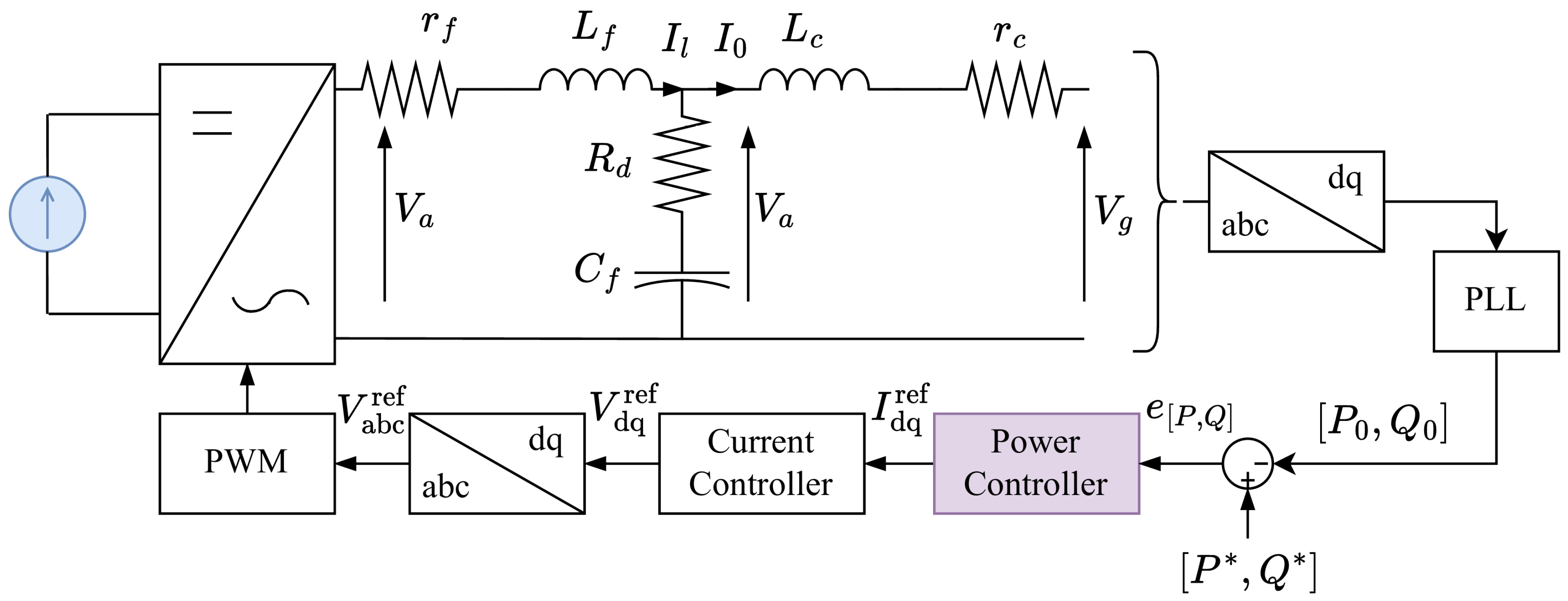
A general GFL control system is shown in Figure 1. GFL inverters are the most commonly deployed type. They operate based on a phase-locked loop (PLL), which estimates and tracks the grid frequency and phase angle at the point of inter-connection (POI) [20]. Their primary function is to maintain pre-set active and reactive power outputs, with limited ability to regulate local frequency or voltage. Consequently, GFLs respond passively to disturbances, adjusting internal references according to external grid signals.

Although both GFL and GFM inverters can emulate virtual inertia and damping, GFM inverters consistently outperform GFLs in terms of frequency nadir improvement and RoCoF mitigation [21]. GFM inverters achieve this with reduced control effort and less synthetic inertia. Studies have shown that while GFL inverters can be enhanced with droop-based frequency control [22], GFM inverters provide more effective support in both frequency and voltage regulation. In particular, GFMs directly regulate terminal voltage and frequency, enabling faster and more accurate responses to grid disturbances.

Given these advantages, it is recommended to allocate GFMs for ancillary services and GFLs for Maximum Power Point Tracking (MPPT) to optimize both energy extraction and grid stability [23]. The power reference tracking behavior of a GFL inverter is described by:

$$0=P^{\ast }-P_e$$

(1)

where P* is the power setpoint, and P_e is the actual power output, indicating that GFL inverters effectively behave as negative loads in the absence of frequency control.

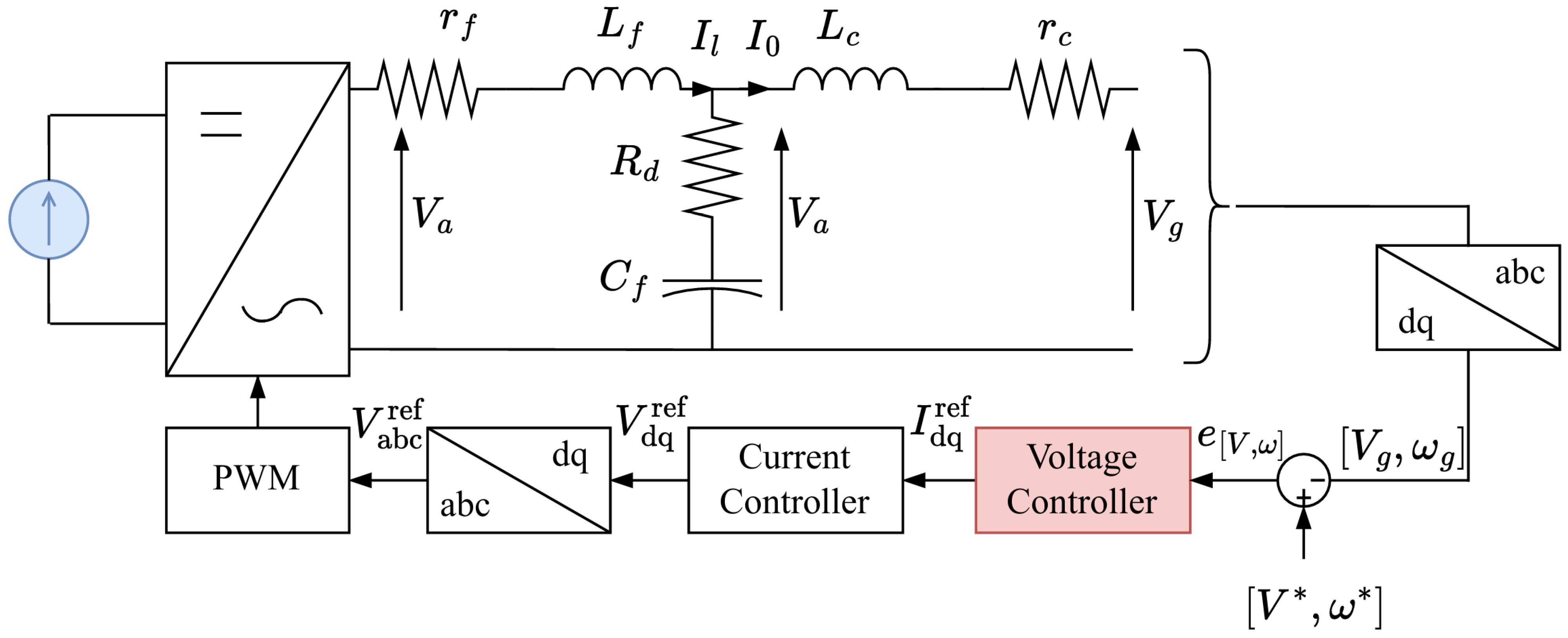
A general GFM control system is illustrated in Figure 2. In contrast to GFL inverters, GFM inverters autonomously establish voltage and frequency at their terminals. They dynamically adjust their internal voltage and frequency in response to deviations in power injection, making them particularly suitable for weak grid conditions or islanded operation scenarios.

A GFM inverter implementing active power droop control with low-pass filtering can be described by the transfer function:

$${\displaystyle \frac{\Delta {\omega }_{\mathrm{GFM}}}{\Delta P_e}}={\displaystyle \frac{R}{T_{{\omega }_c}s+1}}={\displaystyle \frac{R/T_{{\omega }_c}}{s+1/T_{{\omega }_c}}}$$

(2)

where R is the droop gain and $T_{{\omega }_c}$ is the time constant of the low-pass filter. The system has a single real pole at:

$$s_1=-{\displaystyle \frac{1}{T_{{\omega }_c}}}=-{\omega }_c$$

(3)

indicating fast and stable frequency response.

The time domain differential form is:

$$s\Delta {\omega }_{\mathrm{GFM}}={\displaystyle \frac{R}{T_{{\omega }_c}}}\left(\Delta P_e-{\displaystyle \frac{1}{R}}\Delta {\omega }_{\mathrm{GFM}}\right)$$

(4)

which yields the swing equation-like state-space form:

$$\dot{x}=M^{-1}(P^{\ast }-P_e-Dx)$$

(5)

with equivalent inertia and damping identified as:

$$M_{\mathrm{GFM}}={\displaystyle \frac{T_{{\omega }_c}}{R}},\hspace{0.33em}{D}_{\mathrm{GFM}}={\displaystyle \frac{1}{R}}$$

(6)

These parameters demonstrate how droop gain and filter time constant shape the inverter’s synthetic inertial response, reinforcing the suitability of GFM inverters for frequency and voltage regulation in fully inverter-based systems

2.2. Local Frequency Dynamics in IBR-Dominated Power Systems

In IBR-dominated power systems, the local generator-side frequency dynamics can be expressed as:

$$\left\{\begin{array}{l}\Delta {\dot{\delta }}_G={\omega }_0\Delta {\omega }_G\hspace{0.33em}\\ \Delta {\dot{\omega }}_G={\displaystyle \frac{1}{M}}\Delta P_G-{\displaystyle \frac{D}{M}}\Delta {\omega }_G\end{array}\right.$$

(7)

where Δδ_G and Δω_G denote the rotor angle deviation and the frequency deviation, respectively, and ΔP_G is the incremental active power injection. M and D are the equivalent inertia and damping constants. ω₀ = 2πf₀ is the nominal electrical angular frequency, with f₀ being the rated system frequency.

At node i, the active power injection is governed by:

$$P_i=V_i^2{G}_{ii}+{\displaystyle \sum _{j\ne i}{V}_i}{V}_j\left[B_{ij}\sin ({\delta }_i-{\delta }_j)+G_{ij}\cos ({\delta }_i-{\delta }_j)\right]$$

(8)

The linearized power–angle relationship is given by:

$$\Delta P=H\Delta \delta$$

(9)

where H is the Jacobian matrix with elements:

$$H_{ij}=\left\{\begin{array}{ll}-V_i{V}_j\left[B_{ij}\cos ({\delta }_i-{\delta }_j)-G_{ij}\sin ({\delta }_i-{\delta }_j)\right],\hfill & i\ne j\hfill \\ {\displaystyle \sum _{j\ne i}{V}_i}{V}_j\left[B_{ij}\cos ({\delta }_i-{\delta }_j)-G_{ij}\sin ({\delta }_i-{\delta }_j)\right],\hfill & i=j\hfill \end{array}\right.$$

(10)

The system is partitioned into generator (G) and load (L) nodes, where G includes all GFM units, and L includes both conventional loads and GFL inverters, which effectively behave as negative loads in the absence of frequency control:

$$\Delta P=\left[\begin{array}{c}\Delta P_G\\ \Delta P_L\end{array}\right], \Delta \delta =\left[\begin{array}{c}\Delta {\delta }_G\\ \Delta {\delta }_L\end{array}\right],H=\left[\begin{array}{cc}{H}_{GG}& H_{GL}\\ H_{LG}& H_{LL}\end{array}\right]$$

(11)

Substituting into the linearized equation yields:

$$\left\{\begin{array}{l}\Delta P_G=H_{GG}\Delta {\delta }_G+H_{GL}\Delta {\delta }_L\\ \Delta P_L=H_{LG}\Delta {\delta }_G+H_{LL}\Delta {\delta }_L\end{array}\right.$$

(12)

Solving for Δδ_L and substituting:

$$\left\{\begin{array}{l}\Delta {\delta }_L=H_{LL}^{-1}(\Delta P_L-H_{LG}\Delta {\delta }_G)\\ \Delta P_G=\left(H_{GG}-H_{GL}{H}_{LL}^{-1}{H}_{LG}\right)\Delta {\delta }_G+H_{GL}{H}_{LL}^{-1}\Delta P_L\end{array}\right.$$

(13)

Define:

$$H_{\mathrm{red}}=H_{GG}-H_{GL}{H}_{LL}^{-1}{H}_{LG},H_L=H_{GL}{H}_{LL}^{-1}$$

(14)

Then the reduced generator-side relation becomes:

$$\Delta P_G=H_{\mathrm{red}}\Delta {\delta }_G+H_L\Delta P_L$$

(15)

Substituting into the frequency dynamics yields:

$$\Delta {\dot{\omega }}_G=\mathrm{diag}({\displaystyle \frac{1}{M}})(H_{\mathrm{red}}\Delta {\delta }_G+H_L\Delta P_L)-\mathrm{diag}({\displaystyle \frac{D}{M}})\Delta {\omega }_G$$

(16)

The complete state-space form is:

$$\left\{\begin{array}{l}\left[\begin{array}{c}\Delta {\dot{\delta }}_G\\ \Delta {\dot{\omega }}_G\end{array}\right]=\underset{A}{\underbrace{\left[\begin{array}{cc}0& {\omega }_{0}I\\ \mathrm{diag}({\displaystyle \frac{1}{M}})H_{\mathrm{red}}& -\mathrm{diag}({\displaystyle \frac{D}{M}})\end{array}\right]}}\left[\begin{array}{c}\Delta {\delta }_G\\ \Delta {\omega }_G\end{array}\right]+\underset{B}{\underbrace{\left[\begin{array}{c}0\\ \mathrm{diag}({\displaystyle \frac{1}{M}})H_L\end{array}\right]}}\Delta P_L\\ y=\left[\begin{array}{cc}0& 1\end{array}\right]\left[\begin{array}{c}\Delta {\delta }_G\\ \Delta {\omega }_G\end{array}\right]\end{array}\right.$$

(17)

This results in a 2n_G-order linear time-variant (LTV) system, where:

(1)

The state vector comprises n_G rotor angle deviations and n_G frequency deviations.

(2)

The input vector ΔP_L represents load-side active power disturbances.

(3)

The system matrices A and B have dimensions 2n_G × 2n_G and 2n_G × n_L, respectively.

Assuming the reduced Jacobian matrices H_red and H_L are computed based on the pre-disturbance voltage magnitudes and angles, i.e., using V and δ values at the steady-state operating point before any disturbance, the voltage magnitudes are treated as constant, an assumption commonly adopted in analytical frequency studies [24,25]. In weak, low-inertia grids, voltage fluctuations can be significant, but grid-forming inverters with Q–V control can effectively support and stabilize the voltage [26]. Thus, the system can be approximated as a linear time-invariant (LTI) model:

$$H_{\mathrm{red}}={\tilde{H}}_{\mathrm{red}}(V^0,{\delta }^0),H_L={\tilde{H}}_L(V^0,{\delta }^0)$$

(18)

where V⁰ and δ⁰ denote the pre-disturbance voltage magnitudes and angles. It should be noted that, when inverter voltage control is compromised, for example under extreme contingencies or when control inputs reach saturation limits, voltage deviations may become substantial, introducing nonlinear effects that violate the LTI approximation.

From the LTI model, the system modes and spatial–temporal frequency distribution are influenced by the heterogeneity of equivalent inertia M and damping D across nodes. Variations in M and D cause differences in frequency responses Δω_i among nodes, leading to pronounced spatial–temporal patterns.

Additionally, the location and magnitude of load-side disturbances ΔP_L affect how these perturbations propagate through the network via the coupling matrix ${\stackrel{\mathrm{~}}{\mathbf{H}}}_L$. The matrix ${\stackrel{\mathrm{~}}{\mathbf{H}}}_L$ represents the sensitivity of generator nodal power injections to load-side disturbances, which is determined by the network topology and the electrical distance between nodes. Specifically, each element (${\stackrel{\mathrm{~}}{\mathbf{H}}}_L$)_ij indicates the sensitivity of generator i to a disturbance at load j. While it does not directly reflect the instantaneous current distribution, it quantitatively maps load perturbations to generator responses.

Therefore, the uneven distribution of inertia and damping, combined with longer electrical distances within the network, intensifies spatial–temporal frequency variations. Such variations can degrade system stability and increase the likelihood of protection misoperations. The next section proposes mitigation strategies to enhance network coupling and adaptively regulate inertia and damping, thereby improving overall system resilience.

2.3. Mitigation Strategy

Leveraging the state-space formulation derived in previous sections, RoCoF and steady-state frequency deviations are analyzed to inform a mitigation strategy.

Immediately after a disturbance (at t = 0⁺), the frequency and angle deviations are:

$$\Delta {\delta }_G(0^{+})=0,\Delta {\omega }_G(0^{+})=0$$

(19)

This is because Grid-Forming Inverter-Based Resources (GFM-IBRs) emulate physical inertia through their control loops. As a result, the frequency and angle responses exhibit dynamic continuity and cannot change instantaneously, reflecting the behavior of systems with physical inertia. Substituting into the state-space model gives:

$$\Delta {\dot{\omega }}_G(0^{+})=\mathrm{diag}(1/M){\tilde{H}}_L\Delta P_L$$

(20)

This reveals that the initial RoCoF is spatially distributed and determined by the local power disturbance and local synthetic inertia:

$${\mathrm{RoCoF}}_i(0^{+})={\displaystyle \frac{1}{M_i}}{\left({\tilde{H}}_L\Delta P_L\right)}_i$$

(21)

This demonstrates that RoCoF_i(0⁺) depends on the disturbance location and magnitude (ΔP_L), network topology and operating states (${\stackrel{\mathrm{~}}{\mathbf{H}}}_L$), and the synthetic inertia (M_i) of IBRs. Since RoCoF determines the initial rate and direction of frequency change at each location, it significantly influences the overall frequency transient. Section 3.2 will analyze the effect of the disturbance location on frequency dynamics and RoCoF, confirming a strong correlation between spatial–temporal frequency patterns and RoCoF distribution.

At the steady state, time derivatives of frequency deviation vanish:

$$\Delta {\dot{\omega }}_G=0$$

(22)

Thus, the linearized frequency response model reduces to the equilibrium condition:

$${\tilde{H}}_{\mathrm{red}}\Delta {\delta }_G^{\infty }-D\Delta {\omega }_G^{\infty }+{\tilde{H}}_L\Delta P_L=0$$

(23)

The steady-state frequency deviation vector Δ${\omega }_G^{\infty }$ is examined. Suppose the frequencies are not synchronized, i.e., they deviate from a common value. This is expressed as:

$$\Delta {\omega }_G^{\infty }=\Delta {\omega }^{\infty }1+\epsilon ,\mathrm{with} 1^{\mathrm{T}}\epsilon =0$$

(24)

Here, Δω^∞ represents the common (average) frequency deviation, and ε is the deviation from synchronization. The orthogonality condition 1^Tε = 0 ensures a unique decomposition into synchronized and desynchronized components.

Substituting this expression into the equilibrium equation yields:

$${\tilde{H}}_{\mathrm{red}}\Delta {\delta }_G^{\infty }-D(\Delta {\omega }^{\infty }1+\epsilon )+{\tilde{H}}_L\Delta P_L=0$$

(25)

Left-multiplying by 1^T and using the fact that 1^T (since H_red is Laplacian-like), we obtain:

$$H_{\mathrm{red}}={\tilde{H}}_{\mathrm{red}}(V^0,{\delta }^0),H_L={\tilde{H}}_L(V^0,{\delta }^0)$$

(26)

Given that D is diagonal, the term 1^TDε = ∑_iD_iε_i. Since ε satisfies 1^Tε = 0, and D_i > 0, this weighted sum is zero only if ε = 0. Hence, the only solution consistent with the equilibrium condition is:

$$\epsilon =0\Rightarrow \Delta {\omega }_G^{\infty }=\Delta {\omega }^{\infty }1$$

(27)

This demonstrates that the local frequency dynamics achieve synchronization regardless of generator parameters. This property will be further validated through case studies in Section 3.2.

Then, the common steady-state deviation is explicitly given by:

$$\Delta {\omega }^{\infty }={\displaystyle \frac{{\displaystyle {\sum }_i{\left({\tilde{H}}_L\Delta P_L\right)}_i}}{{\displaystyle {\sum }_i{D}_i}}}$$

(28)

Given that steady-state synchronization is guaranteed, the focus is shifted to shaping the transient and steady-state frequency dynamics to enhance spatial resilience and system security.

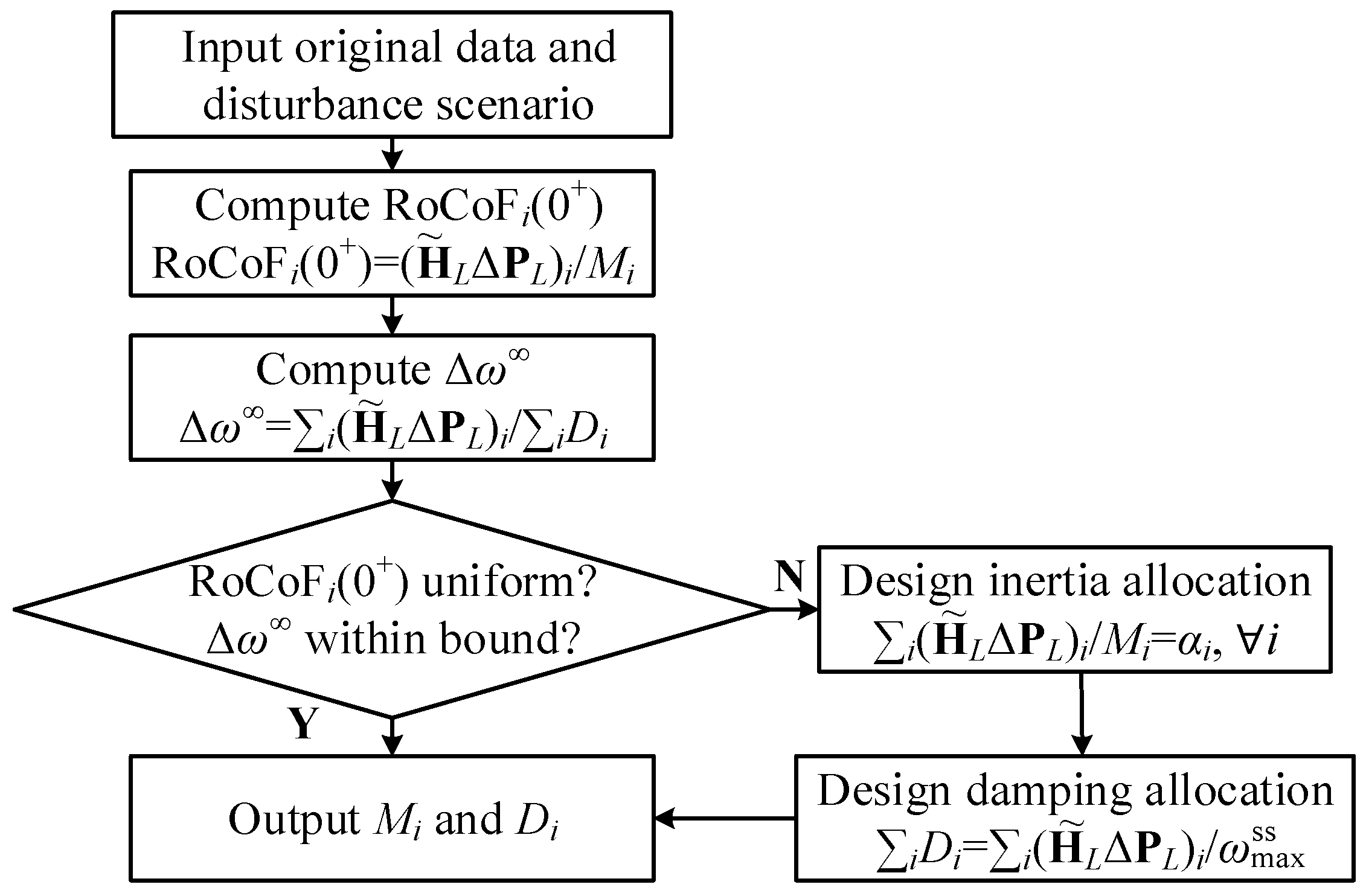
Ensure uniform RoCoF across all nodes at t = 0⁺:

$${\displaystyle \frac{1}{M_i}}{\left({\tilde{H}}_L\Delta P_L\right)}_i=\alpha ,\forall i$$

(29)

where α is pre-defined according to the RoCoF limit (e.g., −2 Hz/s) that ensures each generator proportionally contributes to frequency arrest, thus avoiding spatial imbalances.

Ensure steady-state frequency deviation is within acceptable bounds: to maintain operational security in low-inertia systems, it is essential to limit the synchronized steady-state frequency deviation, given by:

$$\left|\Delta {\omega }^{\infty }\right|=\left|{\displaystyle \frac{{\displaystyle {\sum }_i{\left({\tilde{H}}_L\Delta P_L\right)}_i}}{{\displaystyle {\sum }_i{D}_i}}}\right|\le {\omega }_{\max }^{\mathrm{ss}}$$

(30)

where ${\omega }_{\mathit{max}}^{\mathit{ss}}$ is pre-defined according to the safety frequency threshold (e.g., 0.5 Hz). This criterion directly guides the design of total system damping. To avoid excessive configurations, the total damping requirement can be determined by:

$${\displaystyle \sum _i{D}_i}=\left|{\displaystyle \frac{{\displaystyle {\sum }_i{\left({\tilde{H}}_L\Delta P_L\right)}_i}}{{\omega }_{\max }^{\mathrm{ss}}}}\right|$$

(31)

To ensure consistency and ease of implementation, the damping coefficients D_i are then allocated proportionally to the designed inertias M_i, thus preserving the spatial coordination between inertia and damping.

The overall mitigation framework for shaping spatial–temporal frequency response is illustrated in Figure 3.

The effectiveness of the proposed strategy will be validated in Section 3.3, where case studies consider disturbances at different locations and accordingly design the allocation of inertia and damping across generators to mitigate adverse spatial–temporal frequency patterns.

3. Results

This section presents a series of simulation cases based on the modified IEEE 9-bus and IEEE 39-bus systems to evaluate frequency dynamics under varying conditions. All generation nodes are assumed to be GFM units with a fixed rated capacity of 100 MW providing frequency support; GFL units, if present, would be modeled as load nodes (L) with corresponding updates to the network matrices and state variables. The simulations are organized as follows:

Case 1: Steady-state synchronization, the impact of the disturbance location, and the influence of damping (Section 3.2). Validate the steady-state synchronization property, analyze how the disturbance location influences spatial–temporal frequency dynamics and RoCoF distribution, and study the effect of total system damping scaling on steady-state frequency deviation (Figure 8). Results show that damping has a stronger influence than the disturbance location.

Case 2: Mitigation of spatial–temporal variability (Section 3.3). Generator inertias and damping coefficients are co-designed with respect to the disturbance location. This strategy (i) equalizes initial RoCoF and (ii) limits steady-state deviation, demonstrating effective mitigation.

Case 3: Extension to IEEE 39-bus system (Section 3.4). The proposed framework is applied to the IEEE 39-bus system to assess scalability.

Under 200 MW disturbances at four locations, coordinated parameter tuning improves synchronization and bounds frequency deviations, validating the approach for larger networks.

3.1. Setting

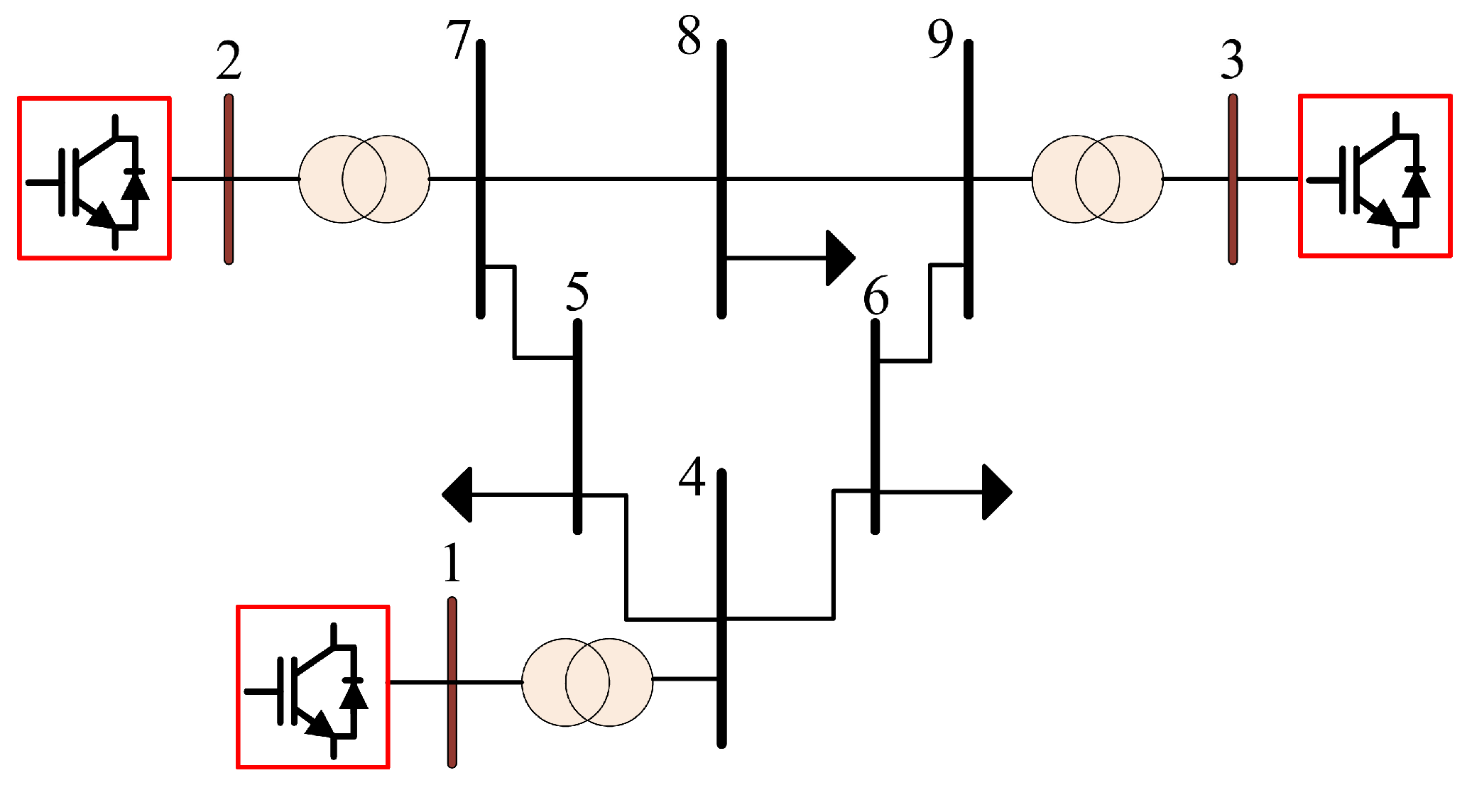
The test system is the modified IEEE 9-bus system, composed of three IBRs, each located at a generator bus. The system has a base capacity of 100 MVA and base voltage of 345 kV. The system layout is shown in Figure 4.

Detailed system parameters including loads, generations, voltages, synthetic inertia, damping values, and branch data are provided in Appendix A.

Each generator is characterized by specific synthetic inertia and damping values, as summarized in

Table 1. M_G and D_G for each generator.

Bus	Synthetic Inertia MG (s)	Damping Coefficient DG (p.u.)
1	6	10
2	3	20
3	1	30

.

3.2. Steady-State Synchronization and Impact of the Disturbance Location

First, the theoretical conclusion that all generator buses eventually synchronize to a common steady-state frequency deviation, regardless of inertia and damping heterogeneity, is verified. Three parameter configurations for IBR units are tested, as summarized in

Table 2. M_G and D_G for the three IBR units.

Setting	MG (s)	DG (p.u.)
1 (baseline)	[6, 3, 1]T	[10, 20, 30]T
2 (equal M)	[3, 3, 3]T	[10, 20, 30]T
3 (equal D)	[6, 3, 1]T	[20, 20, 20]T
4 (equal M and D)	[3, 3, 3]T	[20, 20, 20]T

.

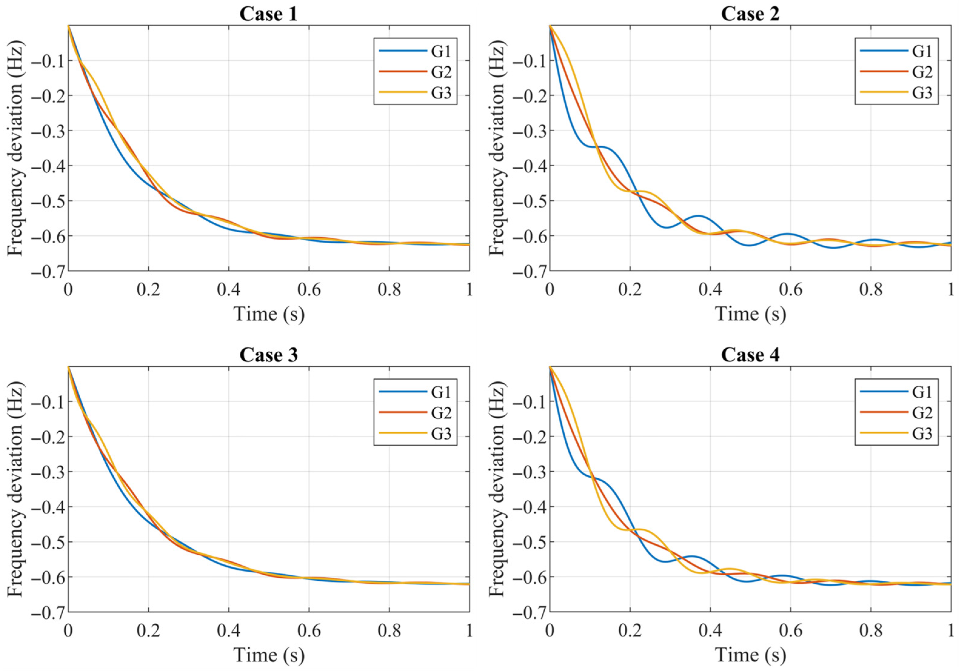
A sudden 60 MW active power load increase is introduced at Bus-5 to simulate a disturbance at t = 0⁺. Figure 5 plots the frequency deviation Δω_i(t) of each IBR unit under the four test settings. In all scenarios, despite significant differences in synthetic inertia and damping, the frequency trajectories converge to a common steady-state value, consistent with the analytical derivation in Section 2.3. This confirms that the steady-state synchronization property is preserved across diverse dynamic parameter configurations.

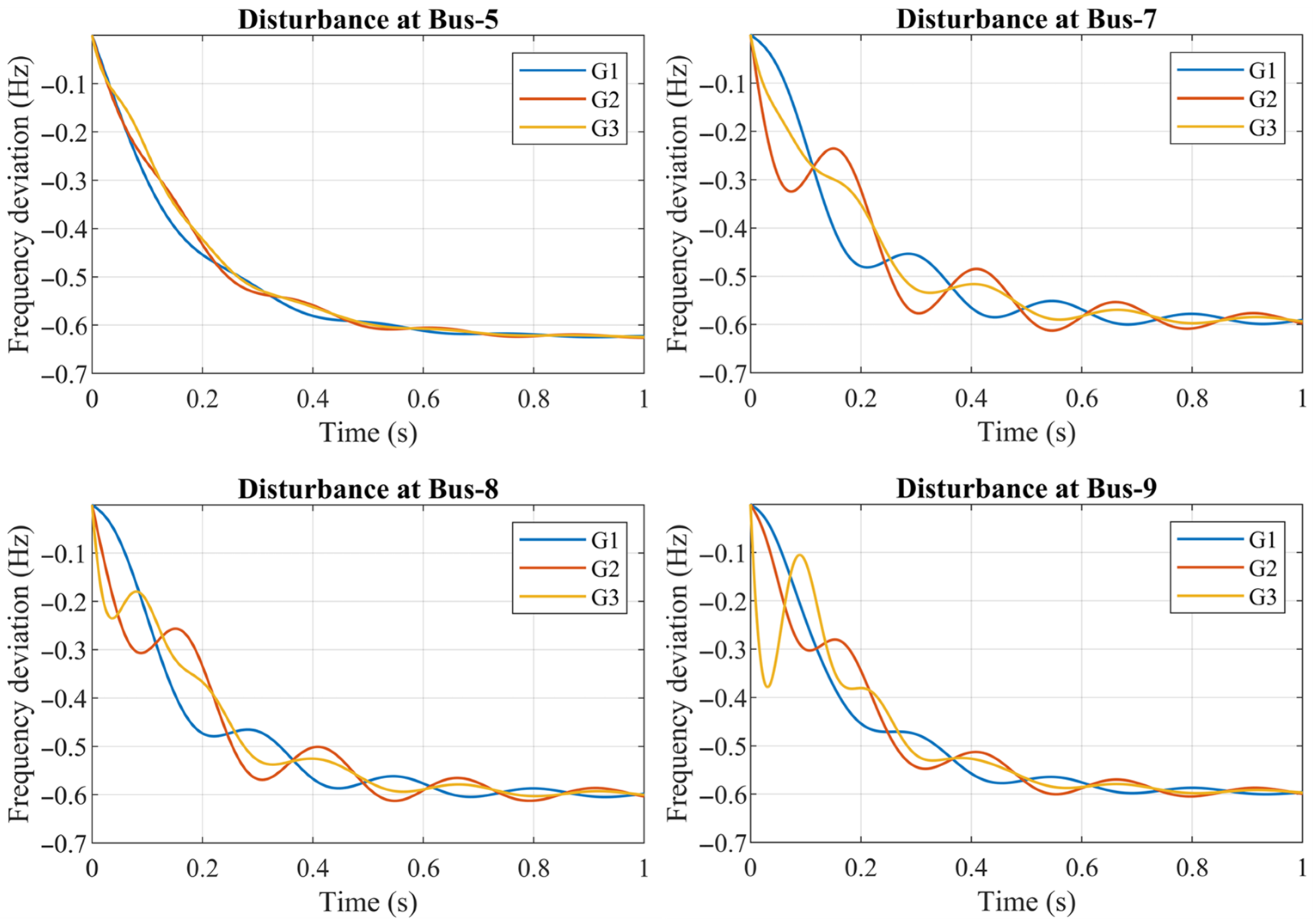
To investigate how the disturbance location influences spatial–temporal frequency dynamics, 60 MW load increases are applied at four different buses (Bus-5, Bus-7, Bus-8, Bus-9) under the baseline parameter configuration (Table 2). The corresponding frequency trajectories are illustrated in Figure 6.

Three statistical metrics are introduced to quantify spatial–temporal differences in frequency dynamics:

Peak Deviation (PD): the maximum absolute deviation of the local frequency from the average frequency trajectory:

$${\mathrm{PD}}_i={\max }_t\left|\Delta {\omega }_i(t)-\Delta \overline{\omega }(t)\right|$$

(32)

Mean Squared Error (MSE): the time-averaged squared deviation:

$${\mathrm{MSE}}_i={\displaystyle \frac{1}{T}}{\displaystyle {\int }_0^T{\left(\Delta {\omega }_i(t)-\Delta \overline{\omega }(t)\right)}^2}dt$$

(33)

Standard Deviation (STD): the standard deviation of the local deviation over time:

$${\mathrm{STD}}_i=\sqrt{{\displaystyle \frac{1}{T}}{\displaystyle {\int }_0^T{\left(\left(\Delta {\omega }_i(t)-\Delta \overline{\omega }(t)\right)-{\mu }_i\right)}^2}dt}$$

(34)

where μ_i = ${\displaystyle \frac{1}{T}}{\int }_0^T[$Δω_i(t) − Δ$\stackrel{\mathrm{-}}{\omega }$(t)]dt is the mean deviation of generator i.

These metrics provide a quantitative measure of the differences in frequency dynamics across generators, with larger values indicating more pronounced spatial–temporal variability.

Table 3. Quantitative comparison of local frequency deviation metrics under different disturbance locations.

Bus	Gen	Peak Dev (Hz)	MSE	STD (Hz)
Bus-5	G1	0.0353	1.0033 × 10−5	0.0031
	G2	0.0220	3.3134 × 10−6	0.0018
	G3	0.0326	5.5950 × 10−6	0.0023
Bus-7	G1	0.1116	1.3506 × 10−4	0.0116
	G2	0.1194	1.0969 × 10−4	0.0105
	G3	0.0326	6.5972 × 10−6	0.0026
Bus-8	G1	0.1107	1.0469 × 10−4	0.0102
	G2	0.0901	6.8299 × 10−5	0.0083
	G3	0.0926	2.7222 × 10−5	0.0052
Bus-9	G1	0.1287	7.6404 × 10−5	0.0087
	G2	0.0912	6.1446 × 10−5	0.0078
	G3	0.2170	1.3114 × 10−4	0.0015

summarizes the results for all four disturbance scenarios. Disturbances at Bus-7, Bus-8, and Bus-9 lead to significantly larger deviations than Bus-5, with Bus-9 exhibiting the largest values, consistent with the frequency trajectories in Figure 6.

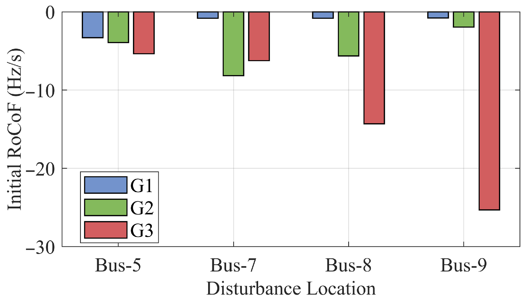
Next, the corresponding RoCoF is analyzed to validate the strong correlation between spatial-temporal frequency patterns and the RoCoF distribution.

Table 4. H_L∆P_L under different disturbance locations.

Gen	Bus-5	Bus-7	Bus-8	Bus-9
G1	−0.3310	−0.0836	−0.0820	−0.0780
G2	−0.1964	−0.4079	−0.2815	−0.0977
G3	−0.0891	−0.1038	−0.2384	−0.4221

summarizes the computed H_L∆P_L vectors for each case, revealing different effective power injections at the generator side due to varying electrical distances.

Next, the initial RoCoF at each bus is calculated as:

$${\mathrm{RoCoF}}_i={\displaystyle \frac{1}{M_i}}{\left({\tilde{H}}_L\Delta P_L\right)}_i$$

(35)

The results are shown in Figure 7. When the disturbance occurs at Bus-5, RoCoF values across generators are nearly identical, and frequency trajectories are closely aligned (Figure 6), showing no obvious spatial–temporal patterns. In contrast, significant RoCoF variations among IBRs lead to pronounced spatial–temporal frequency characteristics, validating the strong correlation between spatial–temporal frequency patterns and RoCoF distribution.

The steady-state frequency deviation is given by:

$$\Delta {\omega }^{\infty }={\displaystyle \frac{{\displaystyle {\sum }_i{\left({\tilde{H}}_L\Delta P_L\right)}_i}}{{\displaystyle {\sum }_j{D}_j}}}$$

(36)

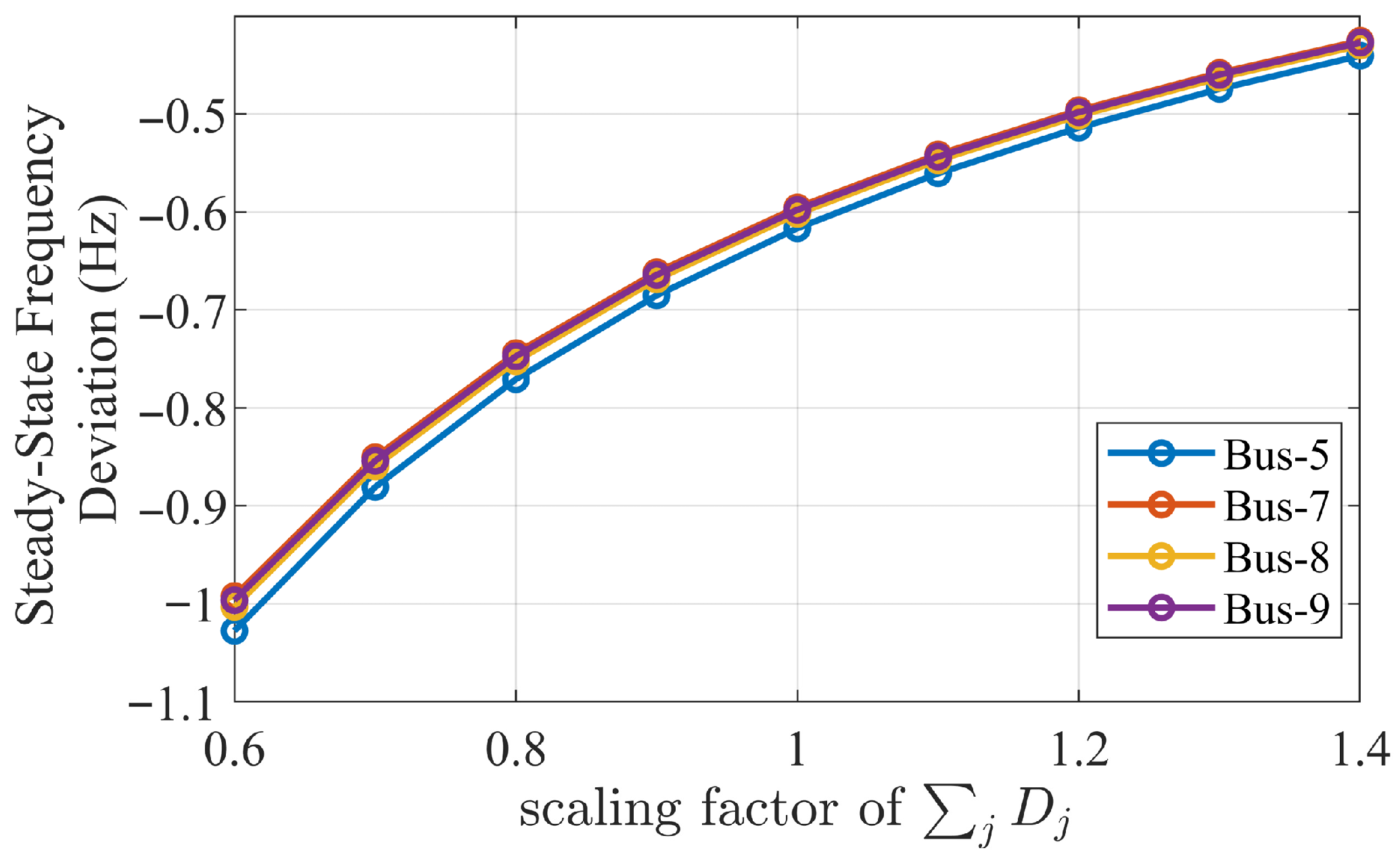
This indicates that Δω^∞ is jointly determined by the aggregated projected power disturbance ∑_i(H_L∆P_L) and the total system damping ∑_jD_j. To quantify their respective influences, the total damping is scaled in steps of ±10% to ±40% around its nominal value, and Figure 8 illustrates the relationship between this scaling factor and Δω^∞ across the four disturbance scenarios. It shows that ∑_jD_j exerts a dominant influence on Δω^∞, while the effect of the disturbance location is negligible.

This phenomenon can be explained by the proposed LTI model: neglecting transmission losses, the aggregated projected power disturbance satisfies:

$${\displaystyle \sum _i{\left({\tilde{H}}_L\Delta P_L\right)}_i}=P_L$$

(37)

where P_L denotes the total load change. As a result, for the same damping scaling factor, the steady-state frequency deviation remains nearly identical across different disturbance locations.

3.3. Spatial–Temporal Frequency Mitigation via Parameter Design

Based on the mitigation framework introduced in Section 2.3, generator parameters are explicitly designed to regulate the spatial–temporal frequency response under four representative disturbance scenarios at Bus-5, Bus-7, Bus-8 and Bus-9. The goal is twofold: (i) enforce uniform initial RoCoF across generators, and (ii) limit the steady-state frequency deviation within a safety bound of ±0.5 Hz.

To align the initial RoCoF, generator inertias M_i are solved for such that:

$${\displaystyle \frac{1}{M_i}}{\left({\tilde{H}}_L\Delta P_L\right)}_i=\alpha ,\forall i,$$

(38)

where α = −2/60 ensures that each generator proportionally contributes to frequency arrest, avoiding spatial imbalances.

To constrain the steady-state frequency deviation within |∆ω^∞| ≤ 0.5 Hz, the total damping requirement is determined as:

$${\displaystyle \sum _i{D}_i}=\left|{\displaystyle \frac{{\displaystyle {\sum }_i{\left({\tilde{H}}_L\Delta P_L\right)}_i}}{{\omega }_{\max }^{\mathrm{ss}}}}\right|$$

(39)

The damping coefficients D_i are then allocated proportionally to the newly designed inertias M_i.

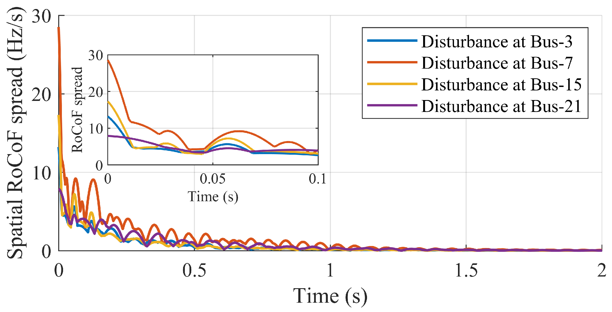
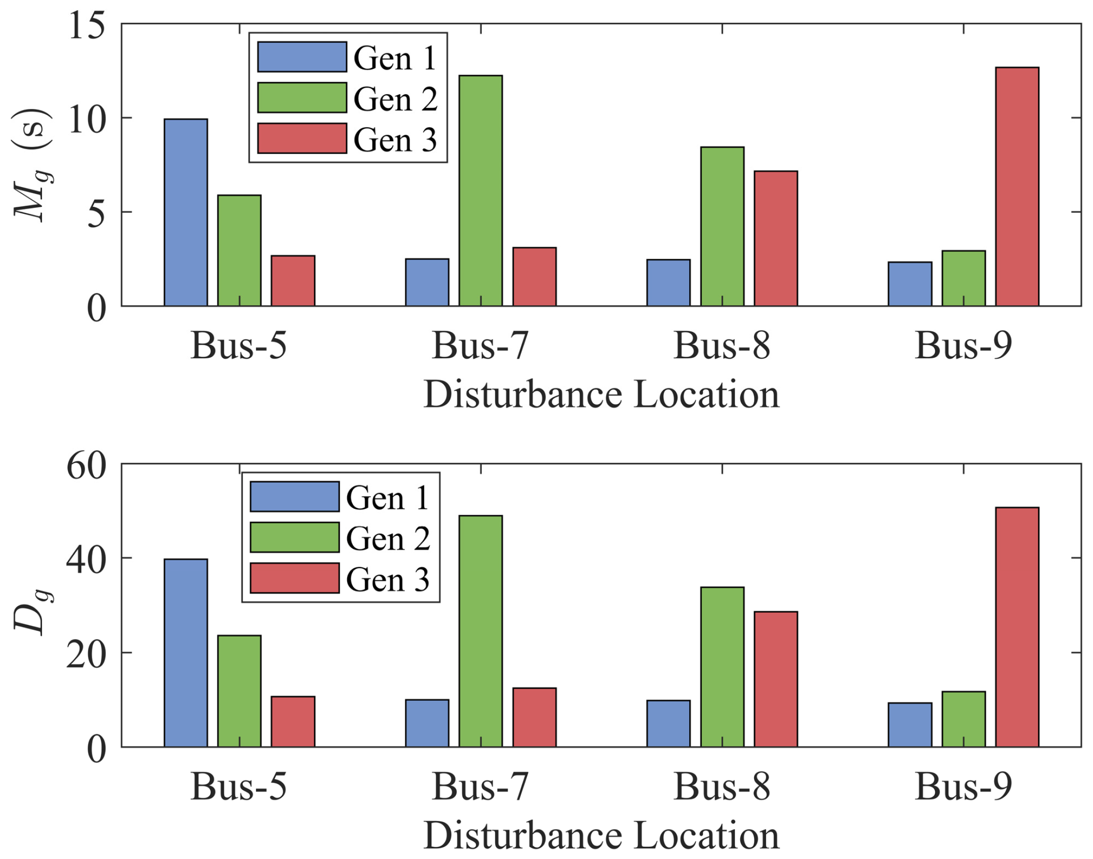
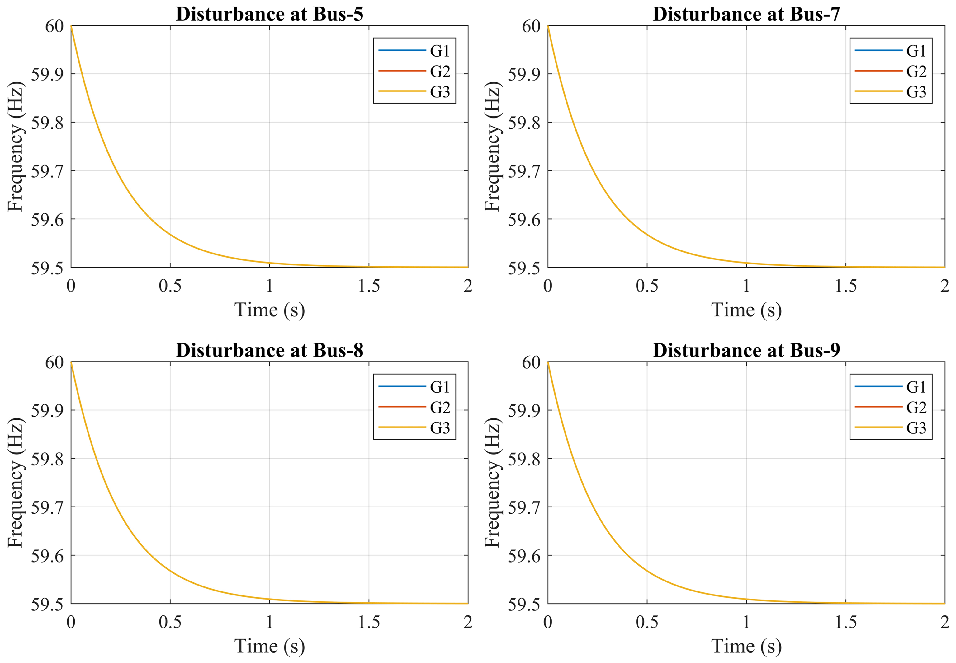
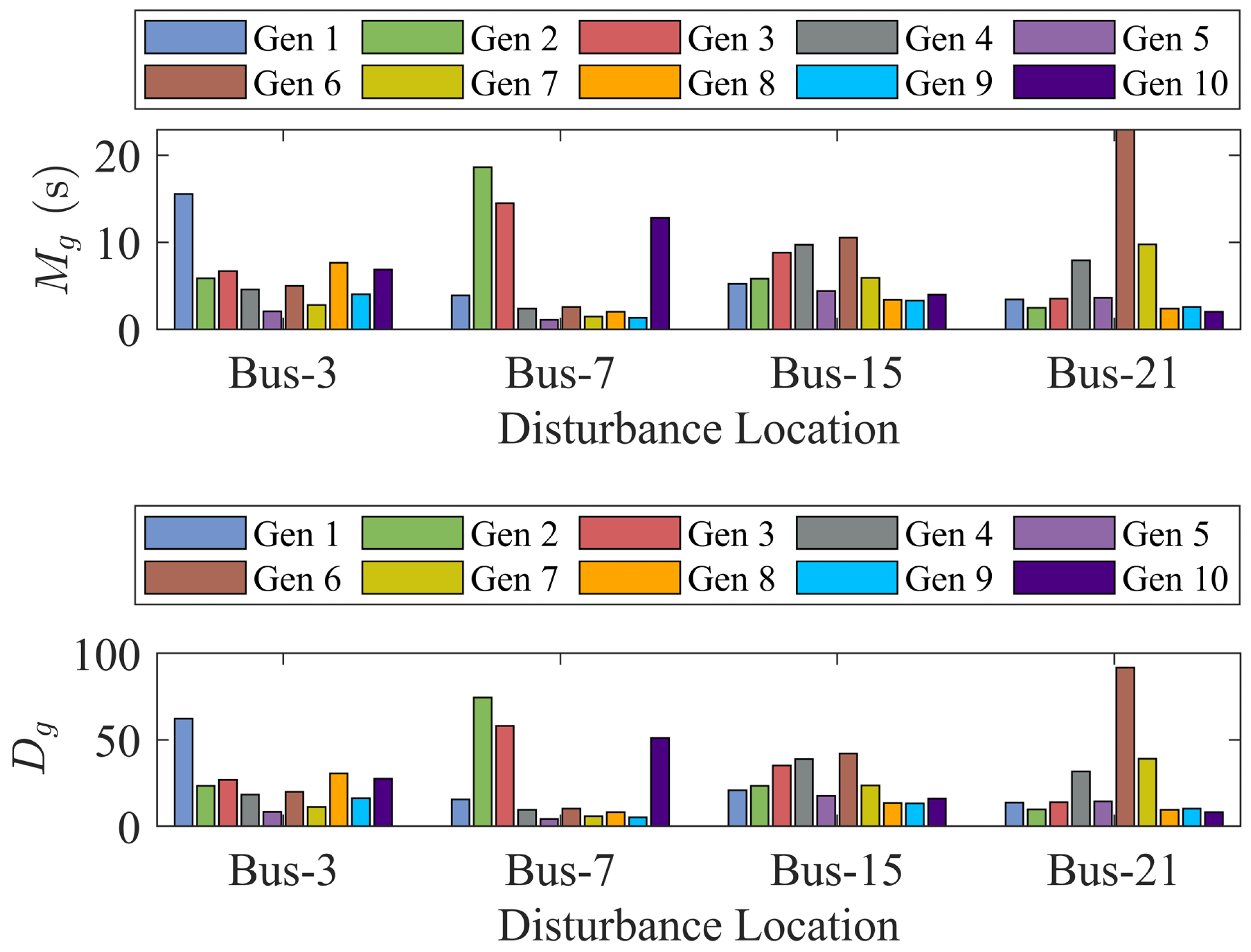
Figure 9 summarizes the designed values of M_g and D_g for each disturbance scenario, illustrating how spatial coordination adapts to the disturbance location.

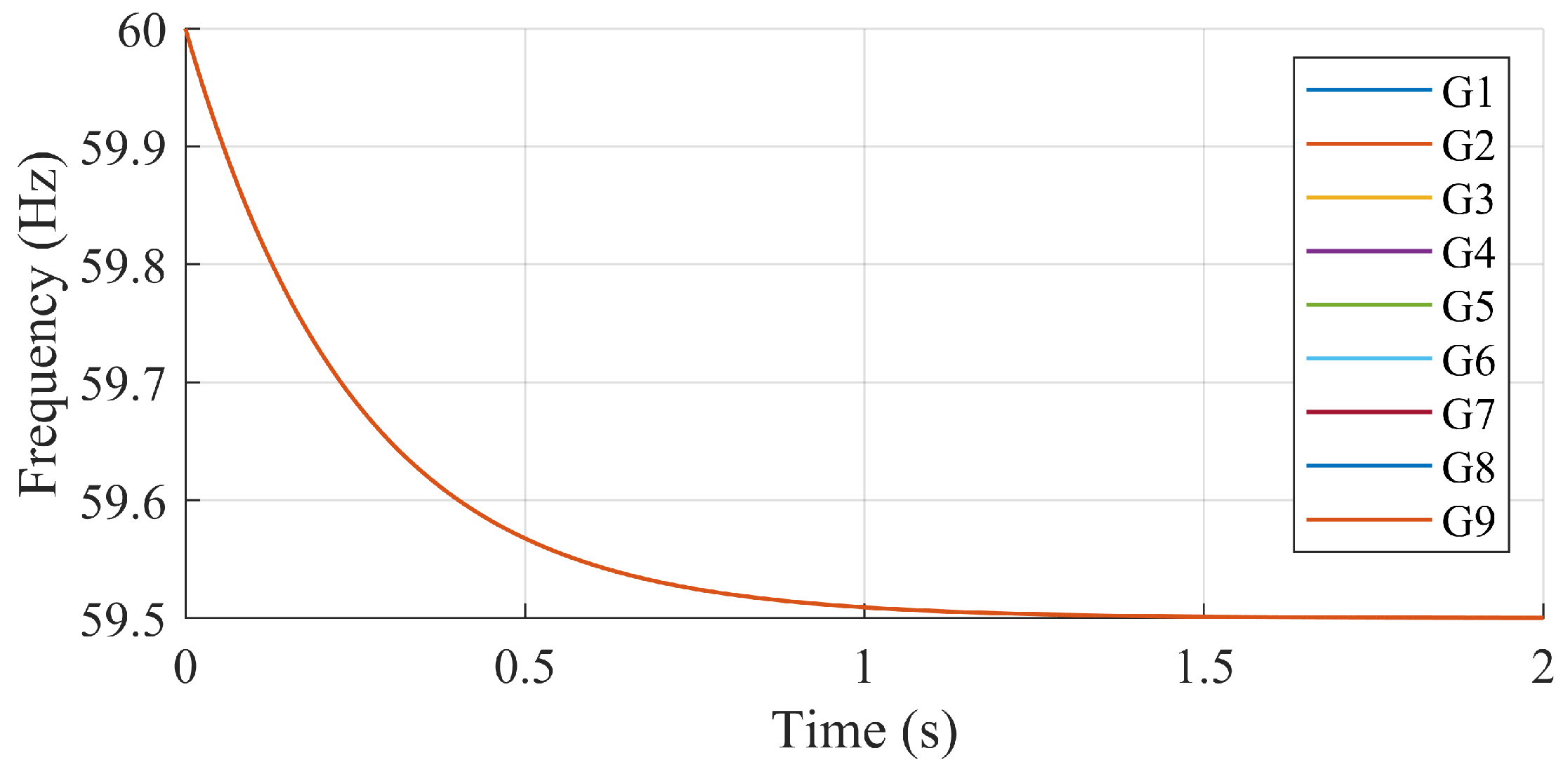
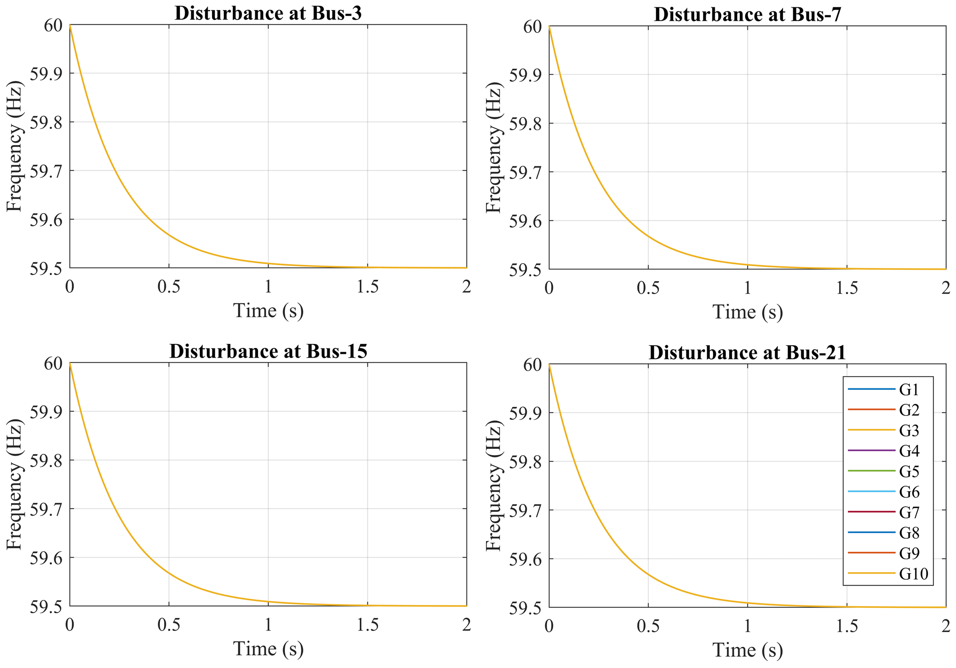
The frequency trajectories following this parameter tuning are shown in Figure 10. All generators exhibit nearly identical RoCoF in the initial transient, and the system converges smoothly to a steady-state frequency of 59.5 Hz, exactly satisfying the design target. This validates the proposed network-aware parameter tuning approach and highlights its capability to coordinate spatial and temporal dynamics in low-inertia systems.

3.4. Extension to Larger System: IEEE 39-Bus Case Study

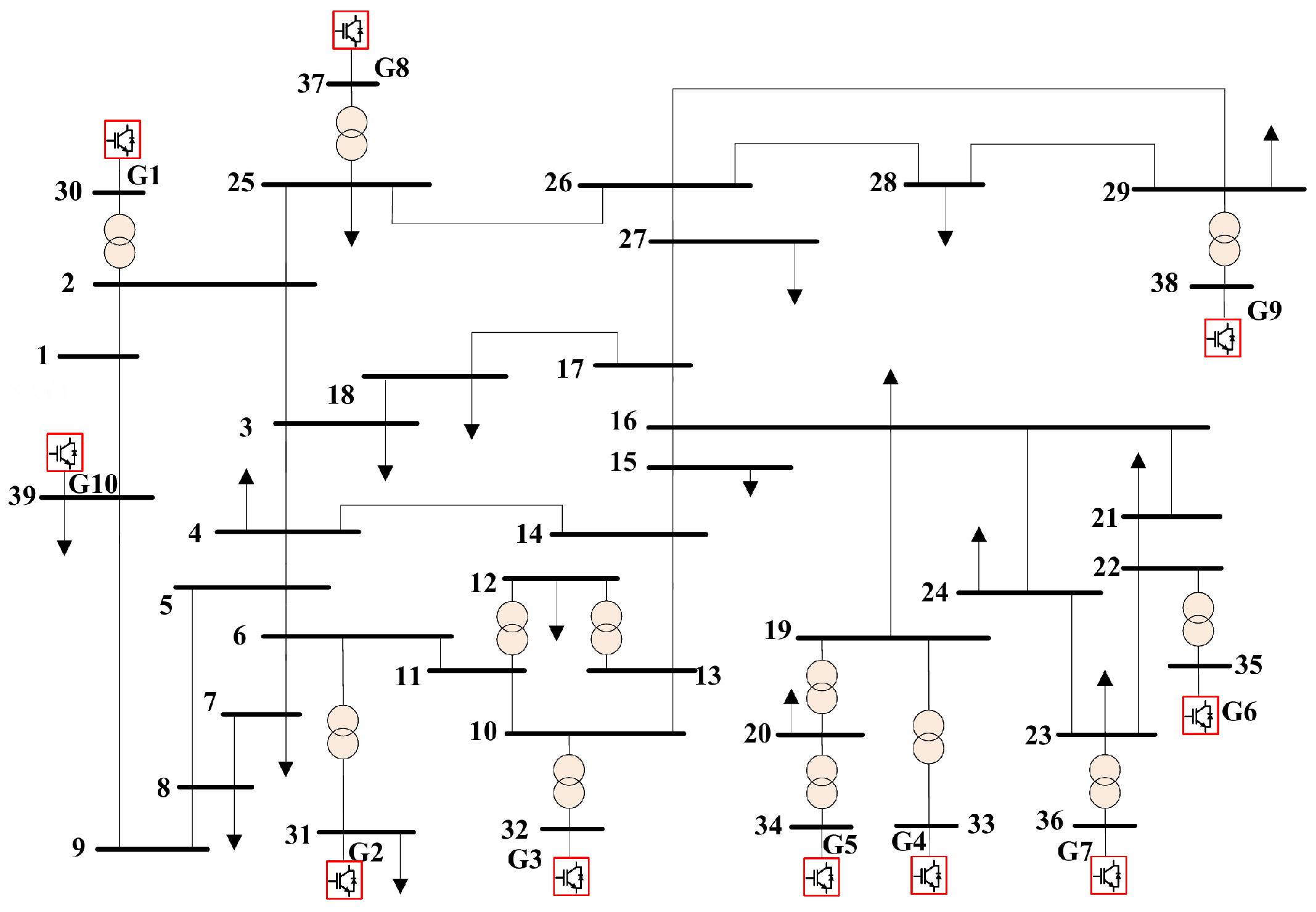
To demonstrate the scalability and applicability of the proposed frequency synchronization and mitigation framework to larger and more complex power systems, simulations are performed on the IEEE 39-bus test system, as shown in Figure 11.

The system includes 10 generator buses (G₁ to G₁₀), each equipped with different synthetic inertia and damping parameters as listed in

Table 5. M_G and D_G for generators in the IEEE 39-bus system.

Bus	Synthetic Inertia MG (s)	Damping Coefficient DG (p.u.)
G1	6.0	20
G2	3.0	13
G3	1.0	30
G4	4.5	28
G5	2.2	12
G6	5.8	15
G7	3.1	18
G8	6.5	22
G9	1.7	25
G10	2.9	40

. Other system parameters of the New England 39-bus system can be found in [27].

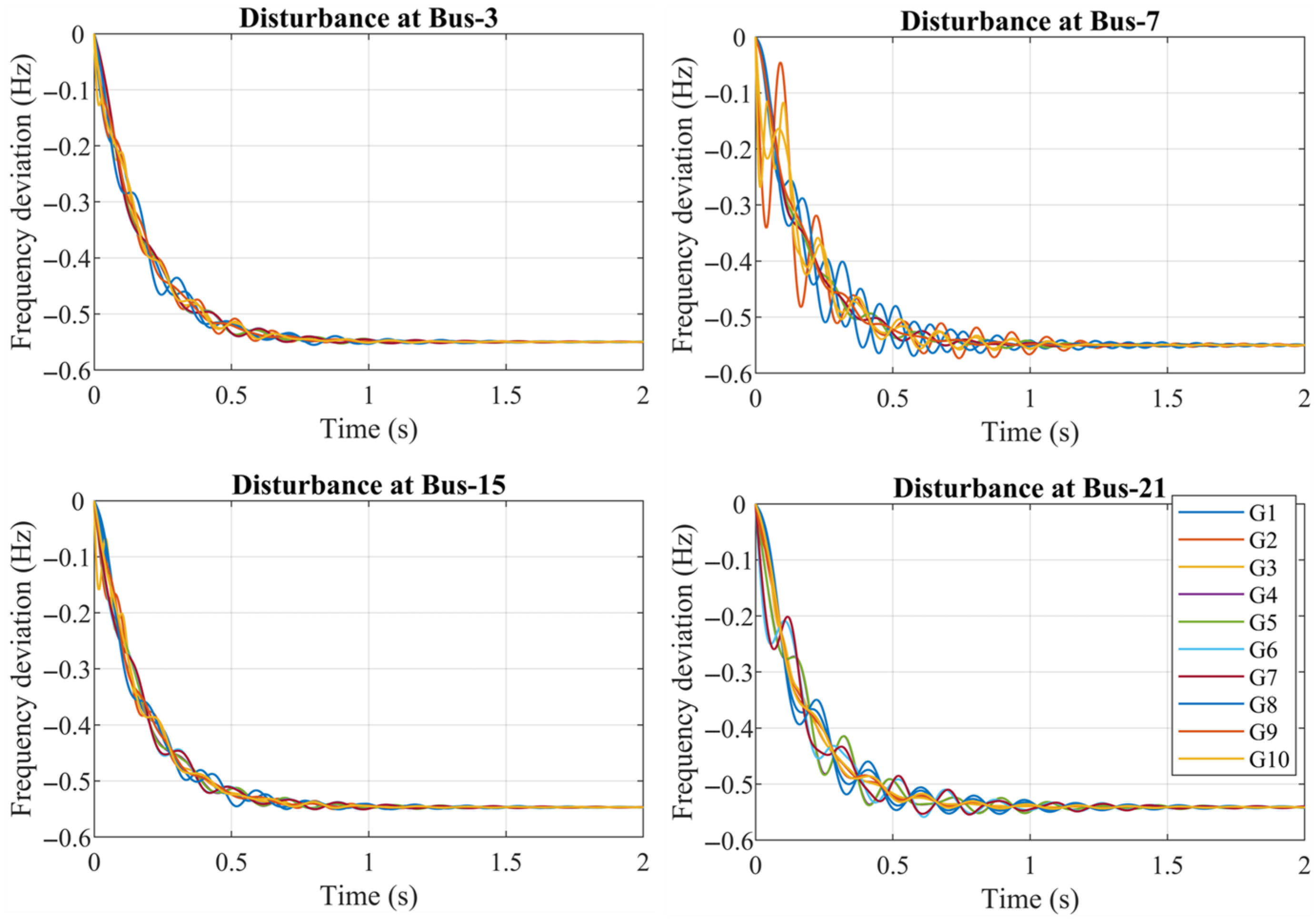
The 200 MW load disturbances are simulated at four different buses: Bus-3, Bus-7, Bus-15, and Bus-21. The resulting frequency deviation trajectories at the generator buses are plotted in Figure 12.

Consistent with the findings from the IEEE 9-bus system, the frequency responses exhibit spatial–temporal variations dependent on the disturbance location, confirming the persistence of these dynamics in larger systems.

Applying the proposed parameter tuning method, the synthetic inertia and damping of each generator are adjusted to mitigate the observed spatial–temporal variations. Figure 13 presents the designed values of M_G and D_G for each disturbance scenario, while Figure 14 shows the resulting frequency trajectories after mitigation. The results demonstrate improved synchronization and effectively bounded steady-state frequency deviations.

To further quantify the effectiveness of the proposed mitigation strategy in suppressing spatial RoCoF imbalance, the RoCoF spread is defined as the difference between the maximum and minimum absolute RoCoF values across all generators at the initial disturbance instant (t = 0⁺):

$$\mathrm{RoCoF} \mathrm{spread}(t)={\max }_i\left|{\displaystyle \frac{f_i(t+\Delta t)-f_i(t)}{\Delta t}}\right|-{\min }_i\left|{\displaystyle \frac{f_i(t+\Delta t)-f_i(t)}{\Delta t}}\right|.$$

(40)

The time domain evolution of the RoCoF spread without mitigation is shown in Figure 15, which provides further insight into the spatial heterogeneity of frequency dynamics prior to control. The results indicate that the RoCoF spread reaches its maximum at the initial instant t = 0 s, immediately following the disturbance, and then rapidly decreases.

Accordingly, the RoCoF spread at t = 0 s is adopted as a worst-case performance metric, and

Table 6. Maximum spatial RoCoF spread at t = 0 s.

Disturbance Bus	Before Mitigation (Hz/s)	After Mitigation (Hz/s)
Bus-3	13.2053	0
Bus-7	28.5327	0
Bus-15	17.2992	0
Bus-21	7.8991	0.7001 × 10−4

compares the RoCoF spread before and after mitigation, quantitatively demonstrating the effectiveness of the proposed mitigation strategy.

This case study demonstrates that the proposed network-aware design approach effectively scales to larger power systems, preserving its ability to coordinate spatial and temporal frequency dynamics under disturbances.

4. Discussion

4.1. Selection of Disturbance Scenario

Since the virtual inertia M_i and damping D_i parameters derived for the proposed mitigation strategy are determined by the power injection vector (${\tilde{\mathbf{H}}}_L$∆P_L)_i, which is directly dependent on the disturbance location, this section elaborates on the practical implementation scheme of the proposed strategy to address this location dependency issue as follows.

The exact location of a disturbance is generally unknown a priori, and it is not feasible to retune inverter control parameters instantaneously following a fault. For practical implementation, the proposed approach can be applied by selecting a representative worst-case disturbance scenario within the dispatch time resolution and tuning the virtual inertia and damping parameters accordingly. For example, the California ISO performs real-time unit commitment with a 15 min resolution [28], within which the outage of the largest online generator can be treated as the representative worst-case contingency. Such a time scale is sufficiently coarse to allow grid-forming inverters to adjust their virtual inertia and damping parameters, given the software-defined and highly flexible control of power electronic converters [23].

Moreover, the state-space formulation models disturbances in the form of power imbalances applied at load buses, i.e., u = ∆P_L. Under generator-trip (N − 1) contingencies, the tripped generator bus can be equivalently represented as a load bus subjected to a step disturbance:

$$\Delta P_{L,k}=P_{e,k}^{\mathrm{pre}}$$

(41)

where $P_{e,k}^{\mathrm{pre}}$ denotes the pre-contingency active power output of the generator. Under this equivalent representation, the proposed parameter tuning strategy remains directly applicable to generator-trip scenarios.

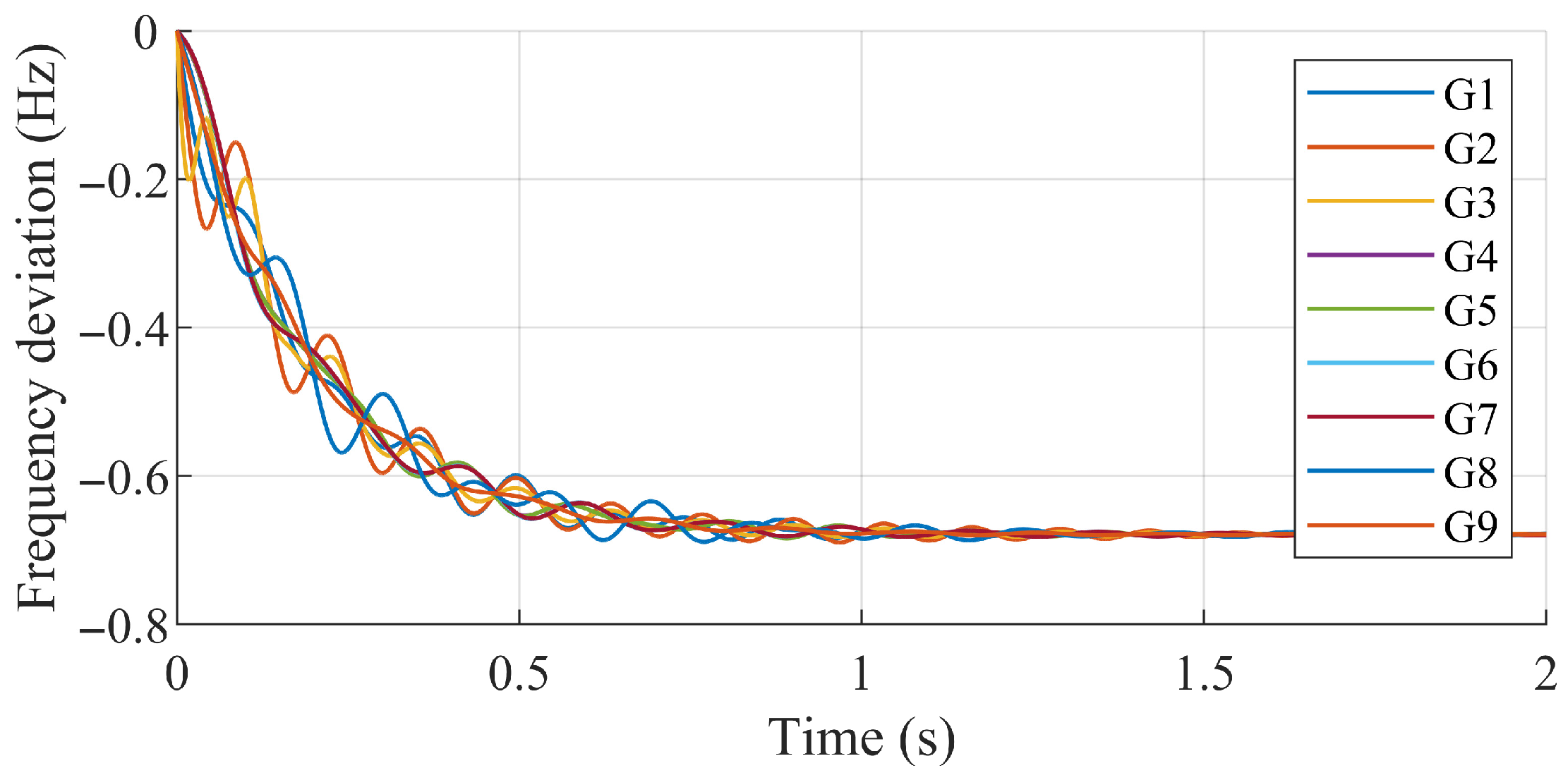
As an illustration, we consider the trip of Generator G10, assumed to be dispatched at 200 MW during the corresponding interval. Figure 16 shows the frequency trajectories of online generators before parameter tuning, while Figure 17 presents the frequency trajectories under the proposed mitigation strategy. The results clearly demonstrate that the proposed approach effectively mitigates spatial–temporal frequency patterns, with spatial frequency variations largely eliminated and overall frequency deviations significantly reduced, confirming the effectiveness of the method under a representative worst-case disturbance scenario.

Furthermore, extending the proposed approach to the real-time adaptive adjustment of virtual inertia and damping based on online measurements is left for future work. Such measurement-based control represents a promising direction to further enhance system resilience under uncertain and fast-varying disturbances, beyond the planning and dispatch-level scenarios considered in this study.

4.2. Practical Constraints on Virtual Inertia Implementation

The proposed RoCoF equilibrium strategy relies on the flexible tuning of virtual inertia parameters. In practical inverter-based resources, however, the achievable level of synthetic inertia is subject to implementation constraints determined by the underlying energy source and converter design. In particular, for GFM battery energy storage systems (BESS), synthetic inertia provision is limited by factors such as the energy capacity, power rating, and fast frequency response capability.

Recent practical deployments indicate that these constraints are not overly restrictive. For example, large-scale GFM BESS projects in Australia have demonstrated that synthetic inertia on the order of 2400 MW can be delivered together with fast frequency response [6]. In this paper, the tuned virtual inertia values for both the IEEE 9-bus and IEEE 39-bus systems result in a maximum inertia constant of 22.9407 s. With a generator capacity of 100 MW, this corresponds to an inertia magnitude of approximately 2290 MW, which is within the range reported in existing GFM BESS implementations.

Nevertheless, it is acknowledged that virtual inertia parameters should be appropriately bounded to reflect hardware limitations in real applications. Incorporating explicit inertia constraints and technology-specific limits into the tuning framework constitutes an important direction for future work.

4.3. Extension to HVDC and Multi-Area Systems

While the proposed parameter tuning strategy has been validated under single-disturbance scenarios, practical power systems often incorporate High-Voltage Direct Current (HVDC) links and multi-area interconnected structures. The demand for frequency dynamic regulation under such complex configurations has not been fully addressed. To broaden the engineering applicability of the framework, this section elaborates on the core ideas and modeling logic for its extension to HVDC and multi-area systems.

HVDC links can provide frequency support through droop control during system faults [29,30]. In the current modeling framework, HVDC is connected to certain generator nodes, and the damping of these generators is increased by D_HVDC, while their inertia remains unchanged. That is, for the set of generator nodes ${\mathcal{G}}_{\mathrm{HVDC}}$ connected to HVDC, the damping is updated as:

$$D_i\leftarrow D_i+D_{\mathrm{HVDC}},\hspace{0.33em}\hspace{0.33em}\hspace{0.33em} \forall i\in {\mathcal{G}}_{\mathrm{HVDC}}$$

(42)

Under this representation, the complete state-space form remains consistent:

$$\begin{array}{l}\left[\begin{array}{c}\Delta {\stackrel{.}{\delta }}_G\\ \Delta {\stackrel{.}{\omega }}_G\end{array}\right]=\underset{A}{\underbrace{\left[\begin{array}{cc}0& {\omega }_{0}I\\ \mathrm{diag}(1/M)H_{\mathrm{red}}& -\mathrm{diag}(D/M)\end{array}\right]}}\left[\begin{array}{c}\Delta {\delta }_G\\ \Delta {\omega }_G\end{array}\right]+\underset{B}{\underbrace{\left[\begin{array}{c}0\\ \mathrm{diag}(1/M)H_L\end{array}\right]}}\Delta P_L\hfill \\ y\hspace{1em}\hspace{1em} =\left[0\hspace{0.33em}\hspace{0.33em}\hspace{0.33em} 1\right]\left[\begin{array}{c}\Delta {\mathbf{\delta }}_G\\ \Delta {\mathbf{\omega }}_G\end{array}\right]\hfill \end{array}$$

(43)

This modeling approach can also be extended to multi-area interconnected systems by appropriately defining generator and load sets for each area and including tie-line power flows in the state-space formulation. A detailed investigation of HVDC and multi-area extensions is beyond the scope of the current paper and is left for future work.

4.4. Impact of GFM/GFL Mixing Ratio

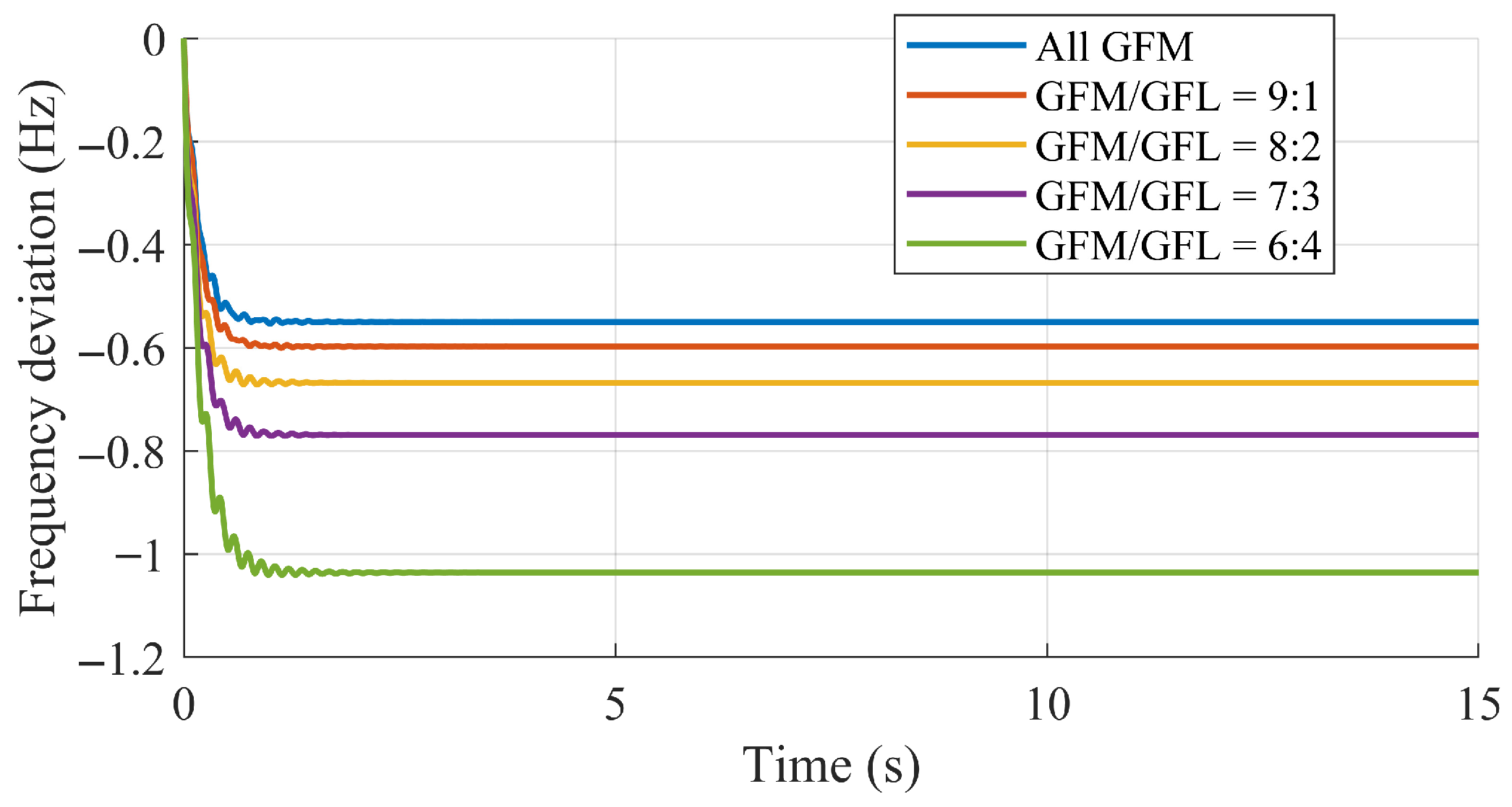
To analyze the impact of a GFM/GFL mixing ratio, additional simulation cases are conducted based on the IEEE 39-bus system, in which the original 10 GFM generators are gradually converted into GFL units at buses 36, 37, 38, and 39. This results in GFM/GFL ratios of 9/1, 8/2, 7/3, and 6/4. A 200 MW disturbance is applied at load bus 3 in each case, and the corresponding frequency dynamics of G1 are shown in Figure 18. As the proportion of GFL units increases, the system experiences larger frequency drops and reduced frequency security, illustrating the critical role of GFM units in providing inertia and frequency support.

5. Conclusions

This paper investigates the spatial–temporal frequency dynamics of low-inertia power systems under disturbances, focusing on IBR-dominated power systems. By leveraging a reduced-order frequency response model and the network response matrix H_L, the disturbance location, network topology, and IBR parameters are characterized to jointly influence key frequency features, including RoCoF and steady-state frequency deviation.

It is analytically proven that, under mild conditions, the system inevitably reaches synchronized steady-state frequency across all generator buses, regardless of parameter heterogeneity. However, transient behaviors such as spatial RoCoF imbalance and unsafe frequency excursions can still arise, particularly when inertia and damping are unevenly allocated.

To address these challenges, a two-pronged mitigation strategy is proposed:

(1)

Adjust synthetic inertia M_i to align initial RoCoFs across all generator buses.

(2)

Configure damping coefficients D_i to ensure steady-state frequency deviation remains within acceptable safety margins.

Simulation results on the IEEE 9-bus system validate the theoretical findings and demonstrate the effectiveness of the proposed spatial–temporal frequency-shaping strategy. For engineering practice, the proposed topology-aware framework features compatibility with mainstream power system planning workflows, relying on core inputs of network topology and inverter parameters; for complex grids with multiple areas or HVDC integration, it can be adapted by extending damping terms and partitioning unit/load sets by area, providing feasible technical guidance for practical application. This work provides actionable insights into frequency security and resilience design in future grid scenarios dominated by IBRs.

Future work will incorporate uncertainty from renewable generation and load forecasts, and develop distributed algorithms for real-time adaptive parameter tuning. In this paper, the proposed tuning strategy is demonstrated for a single representative disturbance scenario. In practical operation, multiple disturbance locations may exist, and the system’s response may vary across them. Future work will extend the proposed approach to consider multiple disturbances, such as weighted-average or worst-case scenarios, to improve robustness against location uncertainty. In addition, future work will also investigate the extension of the method to unbalanced (three-phase asymmetric) networks.

References

1. Shikuma, R.; Orihara, D.; Kikusato, H.; Kaneko, A.; Taoka, H.; Hayashi, Y. Quantitative Difference Between the Effective Inertia and Set Inertia Parameter of Virtual Synchronous Generators. Energies 2025, 18, 1683. [Google Scholar] [CrossRef]
2. Xue, Y.; Li, Z.; Chen, Y.; Zhen, W.; Teng, F.; Strbac, G.; Yang, C.; Tang, W. Sharing of frequency response between asynchronously interconnected systems with renewable generation using LCC-HVDC. CSEE J. Power Energy Syst. 2025, 1–13. Available online: https://ieeexplore.ieee.org/document/10838255 (accessed on 1 February 2026).
3. Tang, W.; Nie, X.H.; Qian, T.; Guo, C.S.; Chen, W.W. Review and Prospect on Application Technologies of Energy Storage for Safety and Stability of New Power System. Guangdong Electr. Power 2024, 12, 3–15. [Google Scholar]
4. Zhang, J.; Xue, Y.; Tang, Y.; Chen, Y.; Chen, M.; He, X.; Lin, S. Equivalent system frequency response model with energy storage. Electr. Power Syst. Res. 2025, 239, 111211. [Google Scholar] [CrossRef]
5. Fang, J.; Li, H.; Tang, Y.; Blaabjerg, F. On the inertia of future more-electronics power systems. IEEE J. Emerg. Sel. Top. Power Electron. 2018, 7, 2130–2146. [Google Scholar] [CrossRef]
6. Homan, S.; Mac Dowell, N.; Brown, S. Grid frequency volatility in future low inertia scenarios: Challenges and mitigation options. Appl. Energy 2021, 290, 116723. [Google Scholar] [CrossRef]
7. Zhao, Z.; Xue, Y.; Chu, Z.; Guo, Y.; Li, Z.; Lin, S.; He, X.; Teng, F.; Strbac, G. Generic Low-order Primary Frequency Response Model for Frequency Nadir Prediction. IEEE Trans. Power Syst. 2025, 40, 5221–5236. [Google Scholar] [CrossRef]
8. Anderson, P.M.; Mirheydar, M. A low-order system frequency response model. IEEE Trans. Power Syst. 2002, 5, 720–729. [Google Scholar] [CrossRef]
9. Shi, Q.; Li, F.; Cui, H. Analytical method to aggregate multi-machine SFR model with applications in power system dynamic studies. IEEE Trans. Power Syst. 2018, 33, 6355–6367. [Google Scholar] [CrossRef]
10. Zhong, Z.; Xu, C.; Billian, B.J.; Zhang, L.; Tsai, S.-J.; Conners, R.; Centeno, V.; Phadke, A.; Liu, Y. Power system frequency monitoring network (FNET) implementation. IEEE Trans. Power Syst. 2005, 20, 1914–1921. [Google Scholar] [CrossRef]
11. Ducoin, E.A.; Gu, Y.; Chaudhuri, B.; Green, T.C. Analytical design of contributions of grid-forming and grid-following inverters to frequency stability. IEEE Trans. Power Syst. 2024, 39, 6345–6358. [Google Scholar] [CrossRef]
12. Ippolito, M.G.; Musca, R.; Sanseverino, E.R.; Zizzo, G. Frequency dynamics in fully non-synchronous electrical grids: A case study of an existing island. Energies 2022, 15, 2220. [Google Scholar] [CrossRef]
13. Ye, K.; Yang, R.; Li, W.; Mo, W. Frequency Stability Analysis and Control Parameter Optimization in High-Voltage Direct Current-Asynchronous Power Systems with Automatic Generation Control. Energies 2025, 18, 864. [Google Scholar] [CrossRef]
14. Zheng, B.; Yang, P.; Jiang, C.; Liu, X.; Hu, Y.; Lei, X. Estimation of Extreme Penetration Rate of New Energy Grid Considering Frequency Constraints. Guangdong Electr. Power 2024, 37, 66–74. [Google Scholar]
15. Trovato, V. The impact of spatial variation of inertial response and flexible inter-area allocation of fast frequency response on power system scheduling. Electr. Power Syst. Res. 2021, 198, 107354. [Google Scholar] [CrossRef]
16. Adrees, A.; Milanović, J.V.; Mancarella, P. Effect of inertia heterogeneity on frequency dynamics of low-inertia power systems. IET Gener. Transm. Distrib. 2019, 13, 2951–2958. [Google Scholar] [CrossRef]
17. Shi, Z.; Xu, Y.; Wang, Y.; He, J.; Li, G.; Liu, Z. Coordinating multiple resources for emergency frequency control in the energy receiving-end power system with HVDCs. IEEE Trans. Power Syst. 2022, 38, 4708–4723. [Google Scholar] [CrossRef]
18. Zhang, Z.; Du, E.; Zhu, G.; Zhang, N.; Kang, C.; Qian, M.; Catalão, J.P. Modeling frequency response dynamics in power system scheduling. Electr. Power Syst. Res. 2020, 189, 106549. [Google Scholar] [CrossRef]
19. Karad, T.B.V.S.; Holjevac, N.; Kuzle, I.; Seppänen, J. Estimation of Area Frequency Response in Island Operation Mode by Utilizing Interconnected Power System Measurements. IEEE Trans. Power Syst. 2024, 40, 1649–1661. [Google Scholar] [CrossRef]
20. Zhang, H.; Xiang, W.; Lin, W.; Wen, J. Grid forming converters in renewable energy sources dominated power grid: Control strategy, stability, application, and challenges. J. Mod. Power Syst. Clean Energy 2021, 9, 1239–1256. [Google Scholar] [CrossRef]
21. Poolla, B.K.; Gro Ss, D.; Rfler, F.D.O. Placement and implementation of grid-forming and grid-following virtual inertia and fast frequency response. IEEE Trans. Power Syst. 2019, 34, 3035–3046. [Google Scholar] [CrossRef]
22. Nguyen, X.H.; Nakajima, T.; Ota, Y. Performance comparison between GFM and GFL inverters in 100% inverter-based power systems. In Proceedings of the 2021 IEEE PES Innovative Smart Grid Technologies-Asia (ISGT Asia), Brisbane, Australia, 5–8 December 2021; pp. 1–5. [Google Scholar]
23. Cui, G.; Chu, Z.; Teng, F. Control-mode as a grid service in software-defined power grids: Gfl vs gfm. IEEE Trans. Power Syst. 2024, 40, 314–326. [Google Scholar] [CrossRef]
24. Rathnayake, D.B.; Akrami, M.; Phurailatpam, C.; Me, S.P.; Hadavi, S.; Jayasinghe, G.; Zabihi, S.; Bahrani, B. Grid Forming Inverter Modeling, Control, and Applications. IEEE Access 2021, 9, 114781–114807. [Google Scholar] [CrossRef]
25. Wang, L.; Ren, J.; Huang, G.; Xie, L.; Feng, C.; Zhang, Y. Identifying the Largest RoCoF and Its Implications. IEEE Trans. Power Syst. 2025, 40, 1164–1167. [Google Scholar] [CrossRef]
26. Wang, J.; Zhang, J.; Hou, Q.; Jiang, H.; Strbac, G.; Teng, F.; Zhang, N. Analytical Decomposition of Nodal Frequency Responses. IEEE Trans. Power Syst. 2025, 40, 1176–1179. [Google Scholar] [CrossRef]
27. Pai, A. Energy Function Analysis for Power System Stability; Springer Science Business Media: New York, NY, USA, 1989. [Google Scholar]
28. California ISO. Tariff Sections: Section 34—Real Time Market. Available online: https://www.caiso.com/documents/section-34-real-time-market-as-of-nov-19-2025.pdf (accessed on 1 February 2026).
29. Li, Z.; Xue, Y.; Fu, Q.; Chen, Y.; Zheng, W.; Yang, C. Low-Frequency Power Oscillations in DC Systems for Asynchronous Interconnection: Insights From the LUXI Back-to-Back HVDC Project. IEEE Trans. Power Syst. 2025, 40, 5446–5458. [Google Scholar] [CrossRef]
30. Li, Z.; Xue, Y.; Chen, Y.; Chen, N.; Yang, C.; Huang, J. Bilateral Primary Frequency Support and AC Voltage Regulation of LCC-HVDC Systems for Asynchronously Interconnected Systems. IEEE Trans. Power Syst. 2025, 40, 2600–2612. [Google Scholar] [CrossRef]
Figure 1. General control system of GFL inverter.
Electronics 15 00813 g001
Figure 2. General control system of GFM inverter.
Electronics 15 00813 g002
Figure 3. Mitigation framework.
Electronics 15 00813 g003
Figure 4. Topology of the modified IEEE 9-bus system.
Electronics 15 00813 g004
Figure 5. Frequency deviation trajectories Δωi(t) of each IBR under different (Mi, Di) configurations.
Electronics 15 00813 g005
Figure 6. Frequency deviation trajectories Δωi(t) of each IBR under 60 MW disturbances at Bus-5, Bus-7, Bus-8, and Bus-9.
Electronics 15 00813 g006
Figure 7. Initial RoCoF at each generator under 60 MW disturbances at Bus-5, Bus-7, Bus-8, and Bus-9.
Electronics 15 00813 g007
Figure 8. Steady-state frequency deviation as a function of the total damping scaling factor under different disturbance locations.
Electronics 15 00813 g008
Figure 9. Designed generator inertias Mg and damping Dg under four load disturbance scenarios.
Electronics 15 00813 g009
Figure 10. Mitigated frequency trajectories after parameter tuning.
Electronics 15 00813 g010
Figure 11. Topology of the modified IEEE 39-bus system.
Electronics 15 00813 g011
Figure 12. Frequency deviation trajectories ∆ωi(t) of generators under 200 MW disturbances at Bus-3, Bus-7, Bus-15, and Bus-21 in the IEEE 39-bus system.
Electronics 15 00813 g012
Figure 13. Designed generator inertias Mg and damping Dg under four load disturbance scenarios.
Electronics 15 00813 g013
Figure 14. Mitigated frequency trajectories after parameter tuning in the IEEE 39-bus system.
Electronics 15 00813 g014
Figure 15. Time domain evolution of the RoCoF spread without mitigation.
Electronics 15 00813 g015
Figure 16. Frequency trajectories of online generators following the trip of G10 before parameter tuning.
Electronics 15 00813 g016
Figure 17. Frequency trajectories of online generators following the trip of G10 after parameter tuning.
Electronics 15 00813 g017
Figure 18. Frequency dynamics of Generator G1 under different GFM/GFL mixing ratios in the IEEE 39-bus system following a 200 MW disturbance at load bus 3.
Electronics 15 00813 g018