Anti-Aliasing for Downsampling in CNNs Based on Gaussian Filter Convolution

Abstract

Convolutional neural networks leverage their efficient ability to extract common features of images, playing a crucial role in numerous computer vision tasks. Key details such as edges and textures in images often present themselves in the form of high-frequency components, which contain rich semantic information and are essential for accurate image recognition and understanding. However, during the downsampling process, these high-frequency components are improperly mapped to low-frequency components, leading to signal aliasing. This aliasing results in the loss of image detail information and blurred features, significantly affecting the precise extraction of image features by convolutional neural networks and ultimately reducing the performance of the model in various tasks. To effectively address this challenge, this study innovatively proposes the Gaussian Filter Convolution (GFC) module. This module ingeniously utilizes convolution kernels with filtering functions, which can specifically suppress the high-frequency components in the image, reducing the occurrence of signal aliasing at its source, thereby significantly alleviating the aliasing artifacts generated during downsampling. Experimental data show that the model integrated with GFC has significant improvements in key indicators such as model accuracy.

1. Introduction

The success of convolutional neural networks (CNNs) in the field of computer vision largely depends on their hierarchical feature extraction mechanism [1]. However, when downsampling layers (strided convolutions or pooling) gradually reduce the resolution of feature maps in this architecture, a critical signal aliasing problem occurs, which affects the stability and generalization ability of the model.

The aliasing effect caused by downsampling operations (including common methods such as pooling layers and stride convolution) has become a key factor leading to the model’s sensitivity to input translations. From a deep theoretical perspective of signal processing, we can conduct an in-depth analysis and find that the feature maps in CNNs can essentially be regarded as a multi-dimensional non-stationary signal that contains rich high-frequency components [2]. These high-frequency components are by no means insignificant; they precisely represent the key detailed features in the image, such as edges and textures. In image information, edges outline the contours of objects, textures reflect the fine structures of the object surfaces, and these high-frequency components are like the “encoding” of these important features, transmitting key information in the form of signals within the feature maps.

According to the classic Nyquist-Shannon sampling theorem [3], in order to completely and without distortion retain all the characteristic information of the signal, the downsampling frequency of the system must strictly follow the basic condition that it must be at least twice the highest frequency of the signal. This theory is like the “golden rule” in the field of signal processing, providing a solid theoretical basis for accurate sampling and retention of signal information. However, in the actual design of CNN architectures, the situation is often not satisfactory. When the downsampling rate (mainly determined by the stride parameter of the convolution operation) cannot meet this theoretical requirement, the phenomenon of spectral folding will occur.

Specifically, when the conditions of the sampling theorem are not satisfied, the high-frequency details, which should be precisely retained in their respective independent frequency bands, are erroneously overlapped into the low-frequency region [4]. This process is akin to forcibly “molding” signals from different frequency bands together, resulting in typical aliasing artifacts. These aliasing artifacts are like “noise” hidden within the signal, seriously interfering with the accurate representation of the original signal.

In the field of deep learning, downsampling, as a key method for data dimension reduction and feature abstraction, can typically be achieved through two mainstream approaches: pooling [5] and stride convolution. The pooling operation aggregates and statistically processes local feature regions to reduce the spatial resolution of the feature map, while stride convolution directly reduces the size of the feature map by employing a stride greater than 1 during the sliding of the convolution kernel.

In the downsampling stage of convolutional networks, the problem of aliasing has always been a key factor affecting the model’s performance. Currently, numerous studies have conducted in-depth exploration on this issue, such as BlurPool, APS, TIPS, AvgPool, and other classic methods that have achieved results. Although these methods can effectively alleviate the aliasing phenomenon, they somewhat neglect its potential impact at the feature extraction level. Previous studies have confirmed that stride convolution, through autonomous learning to adaptively adjust the convolution kernel parameters, demonstrates greater flexibility and feature extraction ability in feature extraction compared to the fixed-rule pooling operation. Additionally, random data augmentation methods also show some anti-aliasing effectiveness to a certain extent. However, most current research focuses on the innovation of anti-aliasing methods in the downsampling process, but few studies start from the unique perspective of pre-filtering high-frequency components before the downsampling operation to solve the aliasing problem.

This study addresses the aliasing artifacts problem in downsampling and proposes and validates an innovative solution. Through a systematic analysis of the information loss mechanism during the downsampling process, we focused on the suppression effect of Gaussian filtering on the high-frequency components during downsampling. Based on this, we proposed introducing Gaussian Filter Convolutional (GFC) before step-size convolutional downsampling to solve the aliasing artifact problem caused by downsampling. Experimental results show that this solution has achieved significant improvements on benchmark datasets such as ImageNet-100, CIFAR10, and CIFAR100. This study provides a new technical path for CNN architecture design, achieving a better balance between computational efficiency and feature retention capability.

Our main contributions can be summarized as follows:

1.

At the theoretical level: We proposed that before downsampling in the stride convolution, applying a Gaussian kernel with filtering capabilities from the frequency domain perspective can effectively alleviate the signal aliasing phenomenon that occurs during downsampling in convolutional neural networks, providing a new theoretical approach to solve the key problems in this field.

2.

In the method design: We innovatively proposed the GFC module, which has excellent compatibility and can be integrated into existing architectures. The parameter quantity only increases by 9, while ensuring an improvement in model performance and almost no increase in computational burden.

3.

In terms of performance: Tested on the ImageNet-100 dataset, the results showed that in key indicators such as accuracy, consistency, and fidelity, it outperformed mainstream comparison methods such as AvgPool, BlurPool, APS, and TIPS.

4.

In terms of universality verification: Experiments were conducted on 4 major architectures including ResNet and MobileNet. This fully demonstrated the wide applicability of the GFC method in different scenarios, laying a solid foundation for its promotion in practical applications.

2. Relevant Work

In the field of deep learning, downsampling is a crucial step in building efficient models. In the early days, pooling operations were the mainstream method for achieving downsampling feature extraction. However, this approach inevitably leads to the loss of some features, which affects the model’s ability to extract features from images.To address these issues, many studies have made improvements and expansions to the pooling operation from different perspectives. Saeedan et al. [6] proposed detail-preserving pooling, which weights the input nodes to enable the model to pay more attention to the important structural information in the image, effectively alleviating the feature loss problem caused by traditional pooling. Boureau et al. [7] analyzed the theoretical basis, influencing factors, and performance of maximum pooling and average pooling, and through empirical comparison, proposed strategies and parameterization methods for optimizing the pooling operation.

Springenberg et al. [8] removed the maximum pooling layer and fully connected layer from the traditional CNN and constructed a network structure consisting only of convolution layers. This network achieved spatial dimension reduction by increasing the stride of the convolution layers, replacing the function of pooling. Experimental results showed that, without data augmentation, this fully convolutional network achieved an error rate of 9.08% on the CIFAR10 dataset. The residual network [9] further adopted this design concept and replaced the traditional pooling with a convolutional layer with a stride of 2 to achieve downsampling. Subsequently, using stride convolution for downsampling gradually became a widely adopted conventional practice in various models [10,11].

In addressing the issue of high-frequency component aliasing during downsampling, Zhang [12] systematically exposed the translational vulnerability problem prevalent in modern CNNs, which stems from the aliasing effect of downsampling. This finding challenges the conventional wisdom that “CNNs inherently possess strong translational invariance” and proposes BlurPool as a solution. BlurPool utilizes low-pass filtering instead of stride convolution for downsampling, significantly enhancing the output stability during image translation.

Ribeiro and Schön [13] demonstrated that the complementary multi-channel information in the intermediate layers of convolutional networks can aid in distinguishing aliasing frequencies; however, aliasing phenomena still persist in these layers. Zou et al. [14] introduced an adaptive perception low-pass filtering layer that dynamically predicts filter weights, achieving a 1.3% performance improvement over ResNet-101 in ImageNet-1K image classification. Chen et al. [15] reduced the probability of frequency aliasing by incorporating anti-aliasing filters, adjusting the downsampling strategy, and utilizing multi-scale frequency fusion within the model, effectively improving the accuracy of image segmentation. Chen et al. [16] proposed spatial frequency decomposition, frequency subband feature extraction, frequency modulation, and fusion, which effectively leverage the frequency information of images, enhancing the performance of semantic segmentation models.

In the context of small target detection tasks, Ning and Spratling [17] observed significant performance improvements in various benchmark models after introducing anti-aliasing technology. Rahman and Yeh [18] proposed the GDEA method, which employs grouping strategies and equivariant anti-aliasing filter design to significantly enhance the performance of CNN models in tasks such as image classification and target detection while preserving the network’s equivariance to specific transformations.

Azulay and Weiss [19] conducted an in-depth analysis of the invariance of convolution operations, pointing out that convolution operations alone cannot guarantee invariance to transformations. They noted that CNNs only learn transformation invariance for highly similar images of typical samples, revealing the fundamental limitations of CNNs when processing transformed images. Vasconcelos et al. [20] addressed the aliasing problem in residual networks through architecture-level position optimization and parameterized experiments, achieving effective suppression of the aliasing issue. This research provides practical methods and insights for optimizing the structure of residual networks and improving their performance. Hossain et al. [21] proposed a novel deep adaptive fuzzy and anti-aliasing activation function, which significantly improved the model’s accuracy under different translational perturbations.

Zhang et al. [22] proposed Spec-ViT, a novel anti-aliasing transformer architecture based on wavelets, which realizes a learnable smoothing factor in the wavelet domain to suppress high-frequency artifacts. Zhang [23] proposed a novel and efficient anti-aliasing network (EAA-Net), which consists of an anti-aliasing context aggregation (AACA) module and a bias channel pruning (PDCP) module. By filtering out the channels severely affected by aliasing, the aliasing effect is suppressed.

Chaman and Dokmanic [24] proposed adaptive polyphase sampling (APS), which generates all possible sub-sampling grids and adaptively selects the grid with the highest energy as the output result, significantly improving classification consistency and making the down-sampled output invariant to translation; Rojas-Gomez et al. [25] proposed a learnable polyphase sampling (LPS) method, by designing end-to-end trainable down-sampling and up-sampling layers, improving the translation invariance and equivariance of convolutional neural networks; Saha and Gokhale [26] proposed translation invariant polyphase sampling (Translation Invariant Polyphase Sampling, TIPS), by decomposing the feature map into multi-phase components at a step size and using learnable mixing coefficients to weight and combine the multi-phase components to suppress the maximum sampling deviation and enhance the model’s translation robustness.

3. Methodology

In convolutional neural networks, the features extracted often contain high-frequency components. These high-frequency components are not insignificant; they precisely correspond to crucial key details such as edges and textures in the image. However, during the downsampling process, the high-frequency components may be mapped to low-frequency components, resulting in a phenomenon known as signal aliasing. Therefore, by applying a convolutional layer with filtering functionality before downsampling and appropriately reducing the high-frequency components, it is possible to more effectively retain the complete feature information during the downsampling process.

Gaussian filtering, as a classic and widely applied linear smoothing filtering technique in the field of image processing, has its core mechanism lying in achieving a delicate balance between noise suppression and edge detail preservation through the weighted average method. From a mathematical perspective, the Gaussian kernel and the convolution kernel have the same calculation mode. Before performing downsampling operations, Gaussian filtering is used to remove the high-frequency components in the image. This measure has two advantages: on the one hand, it can effectively alleviate the aliasing problem caused by high-frequency components; on the other hand, it can fully retain the feature extraction ability of stride convolution. In addition, Gaussian Filter Convolution is implemented by using fixed weights and depthwise convolution, with a small calculation increment and strong compatibility, making it easy to integrate into other models.

The core of Gaussian Filter Convolution lies in that it uses a two-dimensional discrete Gaussian function to generate the weights of the convolution kernel. Unlike ordinary convolution, the weights of Gaussian Filter Convolution are pre-defined and remain constant throughout the model training process, and they are not updated through backpropagation. At the same time, it uses depthwise convolution to complete the corresponding calculation operations. Since the weights of GFC are fixed, all channels use the same Gaussian kernel weight, so the number of parameters of the model only increases by 9 fixed weight parameters.

The calculation forms of the Gaussian kernel and the convolution kernel are consistent, but they have essential differences. During the model training process, the convolution kernel dynamically updates parameters through the backpropagation mechanism to extract features. While the Gaussian kernel can be regarded as a special convolution kernel with filtering functionality. Its weights are fixed values and do not change throughout the training process. This fixed weight characteristic is the core manifestation of its filtering function: by generating a fixed weight matrix using the two-dimensional discrete Gaussian function, the weights remain constant during the training process, thereby avoiding weakening or losing the filtering ability due to weight updates.

The core function of GFC lies in suppressing the high-frequency components in the feature map, thereby effectively alleviating the aliasing phenomenon during downsampling. Essentially, this operation is equivalent to blurring the features extracted by the model. However, it shows significant anti-aliasing effects in the downsampling stage.

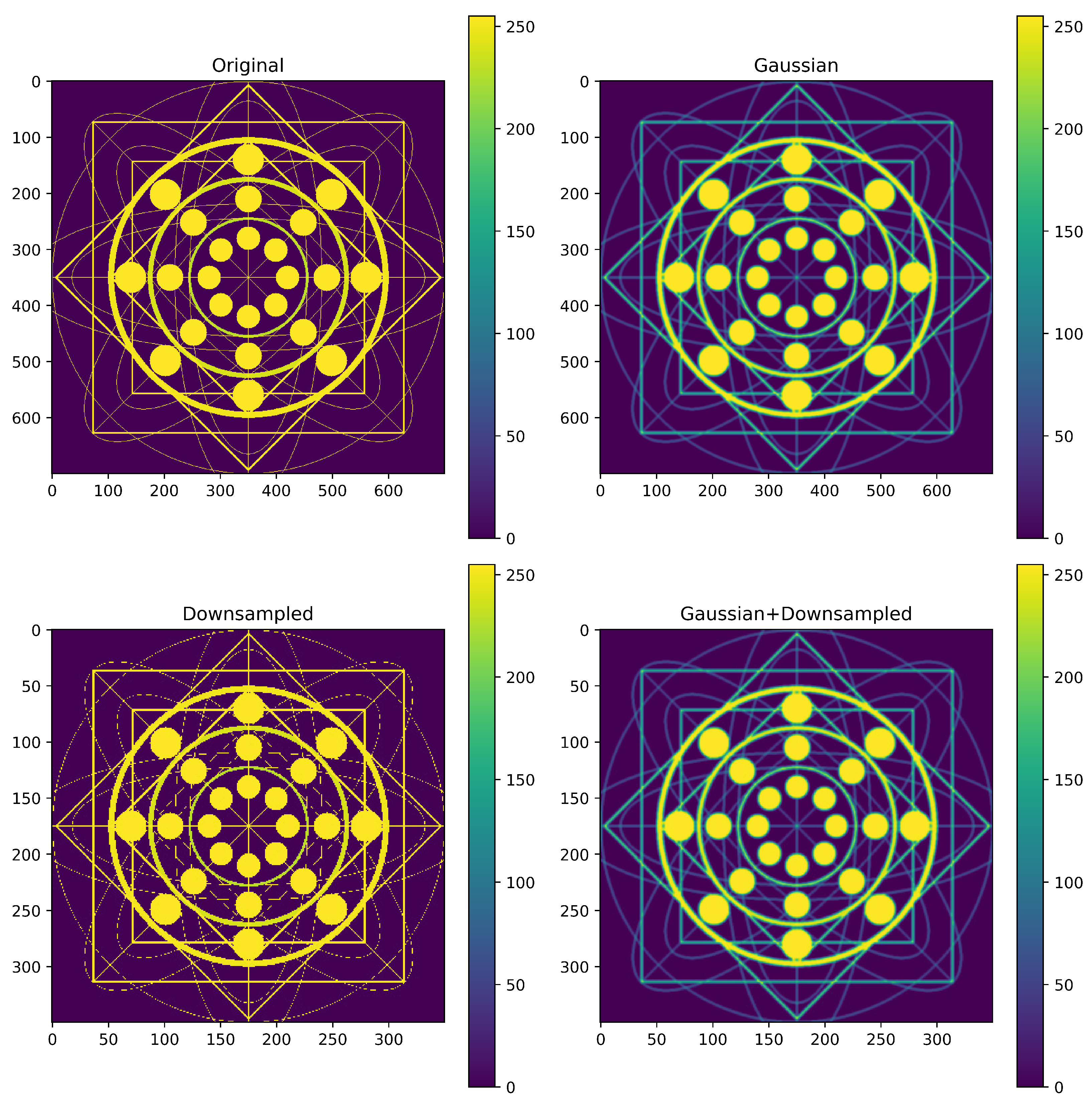
In Figure 1, we conducted a comparative experiment: we performed fixed-point downsampling operations at intervals of one pixel on the original image and the image processed by Gaussian filtering, and presented the results in the form of heat maps. It can be clearly seen that after downsampling the original image, many discontinuities appeared in the lines of the image, and the integrity of the information was damaged; while the original image, after Gaussian filtering, although the image as a whole shows a certain degree of blurriness, after downsampling, it can more completely retain the information contained in the original image.

We implement the Gaussian Filter Convolution function by combining a fixed-weight Gaussian kernel with depthwise convolution. Specifically, first, the corresponding values are generated based on the two-dimensional discrete Gaussian function and then normalized to construct the required Gaussian kernel; subsequently, using the custom Gaussian kernel weights, a Gaussian Filter Convolution is constructed through depthwise convolution. 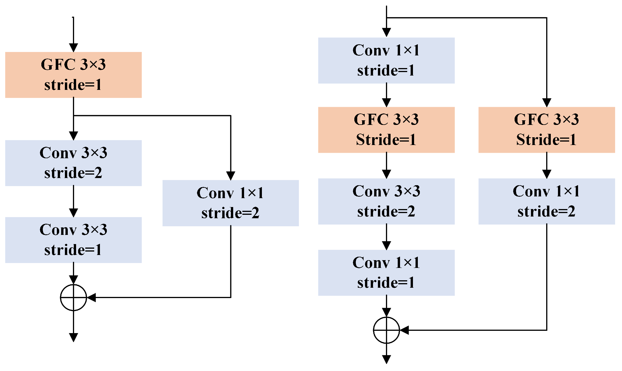Figure 2 shows the fusion method of Gaussian Filter Convolution in the downsampling of two residual networks.

We construct the Gaussian kernel using the two-dimensional discrete Gaussian function. Let the size of the discrete two-dimensional Gaussian kernel be $n\times n$, where $n=2k+1(k\in {\mathbb{N}}^{+})$.The mathematical definition of the two-dimensional discrete Gaussian function is as follows:

$$g(i,j)={\displaystyle \frac{1}{2\pi {\sigma }^2}}{e}^{-{\displaystyle \frac{i^2+j^2}{2{\sigma }^2}}}$$

(1)

The discrete coordinates $(i,j)\in {\mathbb{Z}}^2$ and $(i,j)\in [-k,k]$. $\sigma$ is the standard deviation parameter of the Gaussian distribution. e: the natural constant.

The Fourier transform of the two-dimensional Gaussian function is also a Gaussian function. Due to its separability and rotational symmetry, the two-dimensional Fourier transform is:

$$G(u,v)=\mathcal{F}\left\{g(x,y)\right\}=e^{-2{\pi }^2{\sigma }^2(u^2+v^2)}$$

(2)

The amplitude of the high-frequency component decays exponentially with the square of the frequency. This smooth decay avoids the ringing effect caused by frequency-domain truncation.

$$G(u,v)\propto e^{-2{\pi }^2{\sigma }^2(u^2+v^2)}$$

(3)

The Gaussian filter has the same degree of smoothing in all directions, which makes it free from bias introduced by direction preference in tasks such as edge detection. Since the direction of image edges is usually unknown, rotational symmetry ensures the isotropy of the smoothing operation. In the spatial domain implementation, the Gaussian filter updates the central pixel value through the weighted average of neighboring pixels, and the weights decrease monotonically with the distance from the center point. This local weighting mechanism effectively limits the influence of distant pixels, while suppressing high-frequency components while maximizing the geometric integrity of local features.

From the analysis of its frequency domain characteristics, the Fourier transform of the Gaussian function remains a Gaussian function, and its spectrum exhibits a typical unimodal distribution feature: energy is highly concentrated in the main lobe region, and the amplitude of side lobes decreases exponentially with frequency increase. This spectral structure enables an optimized balance between high-frequency component suppression and feature retention: high-frequency components are effectively filtered out by the main lobe cutoff characteristic, while the low-frequency components and necessary high-frequency details of the image features are retained through the progressive attenuation of the side lobes. Compared to the ideal low-pass filter, the Gaussian filter avoids the ringing effect caused by frequency domain truncation through the smooth transition of the spectrum, significantly improving the robustness of feature extraction.

The smoothing intensity of the Gaussian filter is parameterized by the standard deviation $\sigma$, and it has a positive correlation with the bandwidth: when the $\sigma$ value increases, the filter bandwidth expands, and the smoothing effect strengthens; when the $\sigma$ value decreases, the bandwidth shrinks, and the ability to retain high-frequency details improves. By dynamically adjusting the $\sigma$ parameter, a dynamic balance can be achieved between the feature blurring caused by excessive smoothing and the high-frequency component residue caused by insufficient smoothing, meeting the requirements of different application scenarios.

Then, in order to avoid the imbalance of gradient amplitude, the weights within the kernel are normalized. This is achieved by dividing each weight by the sum of all weights.

$$\widehat{g}(i,j)={\displaystyle \frac{g(i,j)}{{\sum }_{i=-k}^k{\sum }_{j=-k}^{k}g(i,j)}}$$

(4)

$g(i,j)$ represents the original weight of the Gaussian kernel at the position $(i,j)$. The denominator is the sum of all weights, ensuring that the normalized kernel satisfies:

$$\sum _{i,j}\widehat{g}(i,j)=1$$

(5)

Take $\sigma =1.2$ and a Gaussian kernel size of 3 × 3 as an example.

$$\widehat{g}=\left[\begin{array}{ccc}0.0857& 0.1213& 0.0857\\ 0.1213& 0.1717& 0.1213\\ 0.0857& 0.1213& 0.0857\end{array}\right]$$

(6)

After the high-frequency component filtering operation is completed, stride convolution is adopted to achieve downsampling. The following provides the specific mathematical expression to describe the entire downsampling process. Let the input feature map be x. After being processed by the GFC module, $Y_{\widehat{g}}$ is obtained, and its mathematical expression is:

$$Y_{\widehat{g}}=GFC{\left(x\right)}_{\widehat{g}}$$

(7)

To further delve into the related issues, in the experimental part of this study, we selected a 3 × 3 Gaussian kernel size as a typical case for conducting experimental analysis. Subsequently, we employed the stride convolution operation $Poo{l}_{s,k}$, which achieves downsampling by performing a convolution operation with a step size of $s=2$ and a kernel size of $k=3$ on the input feature map, that is:

$$Poo{l}_{s,k}=Conv{\left(x\right)}_{s,k}$$

(8)

Finally, the feature map $Y_{\widehat{g}}$ processed by the GFC module is used as the input for the stride convolution, and the final downsampling output Output is obtained. Its expression is:

$$Output=Poo{l}_{s,k}\left(GF{C}_{\widehat{g}}\left(x\right)\right)$$

(9)

By using the method of first filtering out the high-frequency components and then performing downsampling through stride convolution, the spatial resolution of the feature map is reduced while the key information in the feature map is maximally retained. This reduces the impact of aliasing phenomena on the model performance, thereby improving the performance of convolutional neural networks in various tasks.

4. Experiment

In this study, we conducted experiments using four datasets: Tiny-ImageNet [27], CIFAR10, CIFAR100 [28], and ImageNet-100 [27,29]. Among them, Tiny-ImageNet is a subset of the ImageNet dataset, covering 200 object categories, providing 500 training images for each category (a total of 100,000 images) and 50 validation images (a total of 10,000 images). All images are in a uniform size of 64 × 64 pixels in RGB format. CIFAR10 and CIFAR100 are commonly used image classification datasets in the field of deep learning, both containing a training set of 50,000 images and a test set of 10,000 images, each image being a 32 × 32 pixel RGB color image, covering 10 and 100 categories respectively. The ImageNet-100 dataset is a subset of ImageNet-1K, containing 100 categories. The training set consists of 130,000 images and the validation set consists of 5000 images.

In the experimental setup of this study, for all the datasets and network models used, the stochastic gradient descent (SGD) optimizer was uniformly selected for training. The weight decay coefficient was set to 0.0001, and the momentum parameter was set to 0.9. The initial learning rate was initialized to 0.01, and the learning rate was dynamically adjusted using the cosine annealing strategy [30]. During the adjustment process, the warm restart mechanism was not enabled. At the same time, the batch size was fixed at 128 to ensure the stability and convergence of the training process.

In addition to reporting the top-1 accuracy rate, we used the consistency definition from [14] to compare the prediction results of two shifted images. However, since consistency does not consider the true labels (y) for evaluation, we also used the fidelity definition from [26] as a new metric. Note: $x^{h_1,w_1}$ represents that the image x is vertically shifted by $h_1\sim U(0,{\displaystyle \frac{h}{8}})$ and horizontally shifted by $w_1\sim U(0,{\displaystyle \frac{w}{8}})$. Here, $\mathbb{E}$ and $\mathbb{I}$ represent the expectation and indicator function (output 1 or 0 when the input is true/false). $f\left(\right)$ represents the predicted top-1 category.

$$\mathrm{Consistency}={\mathbb{E}}_{x,h_1,w_1,h_2,w_2}\mathbb{I}[f\left(x^{h_1,w_1}\right)=f\left(x^{h_2,w_2}\right)]$$

(10)

$$\mathrm{Fidelity}={\mathbb{E}}_{x,h_1,w_1,h_2,w_2}\mathbb{I}[y=f\left(x^{h_1,w_1}\right)=f\left(x^{h_2,w_2}\right)]$$

(11)

The experiments were conducted on the ImageNet-100 dataset. The model usually requires the image size to be 224 × 224. The specific approach for using image translation for consistency and fidelity is as follows: we first scale the shortest side of the original image to 256, then crop the image to 256 × 256 based on the image center, and finally randomly select two 224 × 224 images for the calculation of consistency and fidelity. Compared with the cyclic translation method, our translation method is more in line with the actual scenario. In small datasets such as CIFAR10 and CIFAR100, since the image size is smaller, we adopted the method of padding zeros around the image and then randomly cropping it.

4.1. Standard Deviation Analysis

In the two-dimensional discrete Gaussian function, the standard deviation serves as a key parameter that significantly influences GFC. To deeply explore the optimization effect of this parameter in convolutional neural networks, this section conducts systematic experiments based on the ResNet-18 [9] model on the Tiny-ImageNet dataset.

Specifically, we analyze the impact of the standard deviation ($\sigma$) of the two-dimensional discrete Gaussian function on the model performance by adjusting it: The $\sigma$ values are discretized within the range of 0.6 to 2.0 with an interval of 0.2, and 8 different standard deviation experimental variants are constructed; at the same time, three control experiments are set up—(1) the baseline group that retains the original network structure, (2) the control group using the BlurPool [12] method with a blur kernel size of 3 × 3, (3) the alternative method group using mean filtering. Through multiple group comparative analyses, we aim to determine the optimal standard deviation parameter value for GFC under the given model structure.

To more accurately evaluate the performance improvement and effect differences brought about by the proposed improvement methods, we did not use data augmentation techniques in this experiment. The maximum number of iterations was set to 60. The data in the last row “Mean” is the result of mean filtering. Readers can use a 3 × 3 pooling kernel with a stride of 1 for AvgPool to quickly verify the method we have proposed.

Based on the experimental data presented in

Table 1. Accuracy rates under different standard deviations. Mean represents the result obtained through mean filtering. Each model was run independently 5 times and presented in the form of “mean ± standard deviation”.

Model		Top-1 Acc (%)
Baseline		$43.53\pm 0.15$
BlurPool		$49.37\pm 0.34$
GFC	$\sigma =0.6$	$50.46\pm 0.28$
	$\sigma =0.8$	$52.27\pm 0.29$
	$\sigma =1.0$	$53.34\pm 0.18$
	$\sigma =1.2$	$53.43\pm 0.27$
	$\sigma =1.4$	$53.05\pm 0.14$
	$\sigma =1.6$	$52.98\pm 0.31$
	$\sigma =1.8$	$52.60\pm 0.24$
	$\sigma =2.0$	$52.94\pm 0.16$
Mean		$52.41\pm 0.26$

, it can be clearly observed that, compared to the baseline model ResNet-18 that we selected, the GFC module has demonstrated significant performance improvement under different standard deviation $\sigma$ values. Specifically, when the parameter $\sigma$ takes a value greater than 0.8, the accuracy rate achieved by this model in the classification task can remain stable at over 52%. Further comparison reveals that, under all the different standard deviation settings selected, the experimental results obtained by the new model are superior to the BlurPool [12] method.

In particular, it is worth noting that when $\sigma$ takes a value of 1.2, the model exhibits the most outstanding performance, reaching a relatively high accuracy level. However, when the value of $\sigma$ continues to increase and exceeds 1.2, the model’s performance will experience a slight decline to some extent. We speculate that this is due to the excessive smoothing of the filtering effect caused by the excessively large $\sigma$ value, which to some extent loses the details of the image.

We believe that in the field of image processing, the high-frequency components constitute the precise mathematical expression of key visual features such as edge sharpness and texture details within the image. Moderate suppression can enhance the model’s anti-aliasing ability, but excessive suppression of these high-frequency components will not only reduce the visual richness of the image itself, but may also have a significant negative impact on the feature extraction ability and expression efficiency of the subsequent model. Therefore, when $\sigma$ is greater than 1.2, the accuracy rate of the model will decrease.

Based on the above experimental observations and in-depth analysis, in the subsequent experimental research, we will uniformly set $\sigma$ as 1.2 as the basic parameter setting for further exploration and optimization of the model performance.

4.2. Experiment on ImageNet-100

To verify the effectiveness of the proposed method, we conducted a comparative experiment on the ImageNet-100 dataset. We used the original ResNet-50 [9] as the baseline model and combined it with the GFC module proposed in this paper, along with three representative anti-aliasing methods: AvgPool, BlurPool [12], APS [24], and TIPS [26]. The size of the BlurPool blur kernel was 3 × 3.

We employed two experimental setups to comprehensively evaluate the model performance: Firstly, without using data augmentation, only the original images were used for training and testing. This setup was designed to purely examine the inherent feature extraction capability of the model architecture under no external intervention conditions, with the number of iterations set to 60; Secondly, data augmentation was introduced as a comparative experiment. Specifically, the conventional enhancement strategies of random cropping and scaling (RandomResizedCrop) and random horizontal flipping (RandomHorizontalFlip) were applied to the input images. The number of iterations was set to 160. Each model was run independently 3 times and the results were presented in the form of “mean ± standard deviation”. Data augmentation, through spatial distribution randomization operations, can indirectly alleviate the aliasing effect that occurs during downsampling. On this basis, we further compared the adaptability of different anti-aliasing methods to the changes in feature diversity in the data augmentation environment, as well as the resulting performance gain differences.

In

Table 2. Comparison of anti-aliasing methods on the ImageNet-100 dataset. “w/o augmentation” represents not using data augmentation techniques, while “w/augmentation” indicates the use of common data augmentation techniques.

Model	w/o Augmentation			w/Augmentation
	Accuracy	Consistency	Fidelity	Accuracy	Consistency	Fidelity
Baseline	63.20 ± 0.24	70.32 ± 0.26	55.82 ± 0.30	81.09 ± 0.38	92.22 ± 0.27	78.41 ± 0.26
BlurPool	69.18 ± 0.11	84.26 ± 0.10	64.46 ± 0.13	80.46 ± 0.09	93.36 ± 0.10	78.35 ± 0.12
APS	67.90 ± 0.26	82.04 ± 0.19	62.34 ± 0.21	79.45 ± 0.11	91.56 ± 0.32	76.54 ± 0.16
AvgPool	71.38 ± 0.10	85.82 ± 0.12	67.20 ± 0.12	78.66 ± 0.13	91.30 ± 0.10	75.92 ± 0.15
TIPS	73.38 ± 0.13	85.56 ± 0.20	68.68 ± 0.18	82.11 ± 0.14	93.09 ± 0.05	79.53 ± 0.29
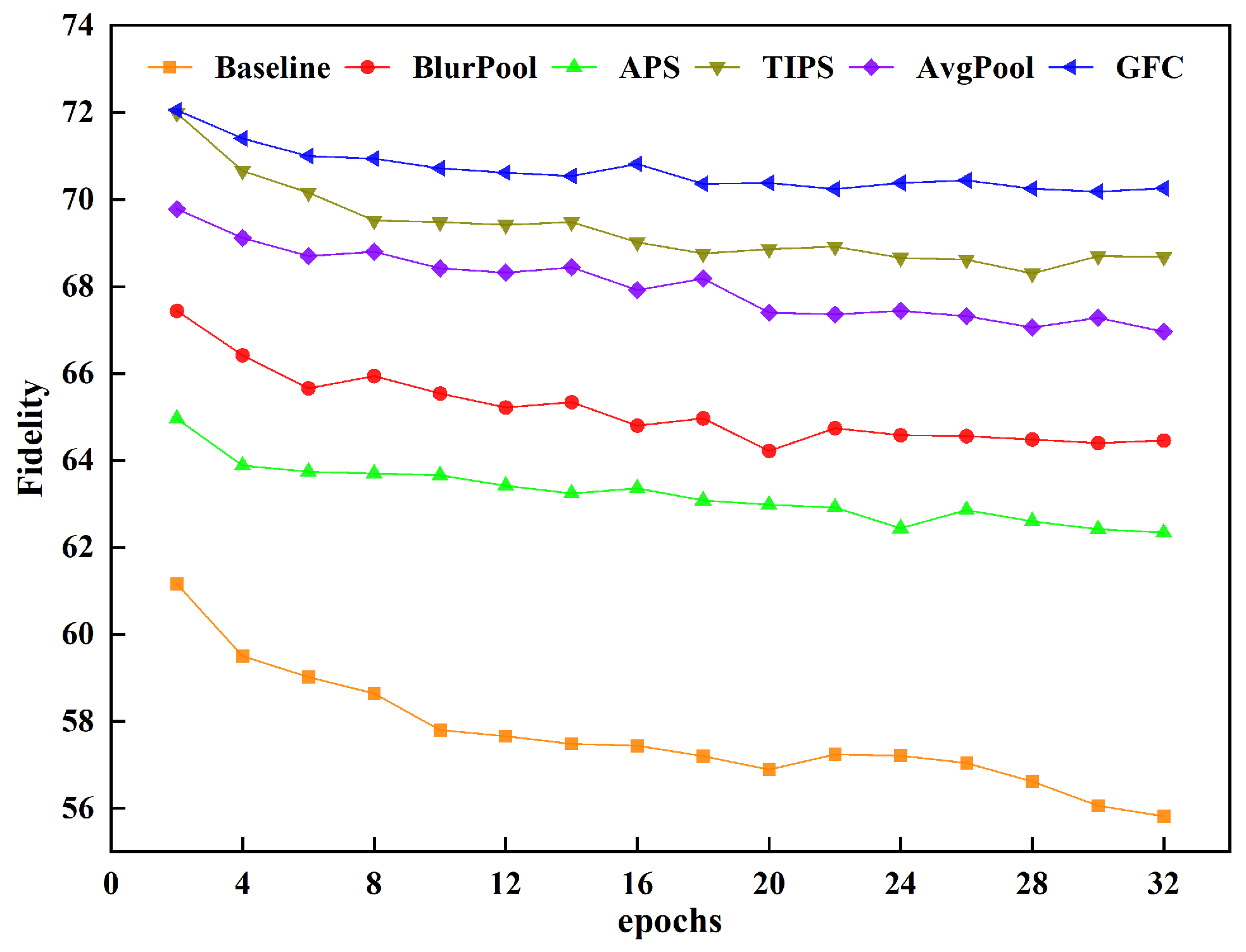
GFC	73.64 + 0.23	88.62 ± 0.18	70.26 ± 0.26	82.06 ± 0.30	94.30 ± 0.19	80.18 ± 0.30

, we conducted a systematic comparative study on different anti-aliasing methods. The research results show that, under the experimental conditions without data augmentation, the anti-aliasing methods exhibit extremely outstanding effects in terms of the feature extraction capabilities of the model itself. Through further in-depth comparative analysis, compared with the existing BlurPool, APS, and TIPS modules, the innovative Gaussian Filter Convolution improved model proposed in this paper demonstrates significant advantages in the three core indicators of accuracy, consistency, and fidelity. In Figure 3, we further compared the changes in fidelity under different translation ranges. Compared with other methods and baseline models, the GFC proposed by us has more stable performance and higher fidelity in different translation ranges.

The classic methods such as BlurPool, APS, TIPS, and AvgPool have all achieved certain results. Although these methods can effectively alleviate the aliasing phenomenon, they tend to ignore the potential impact of this phenomenon at the feature extraction level. In convolutional neural networks, feature extraction is a crucial step, directly determining the model’s understanding and representation ability of the input data. However, the aforementioned classic low-pass filtering methods often adopt fixed filtering rules, and during the smoothing processing of images, they may indiscriminately filter out some information beneficial for feature extraction, thereby limiting the performance improvement of the model in complex scenarios.

Previous studies have confirmed that stride convolution has unique advantages in feature extraction. Stride convolution can adaptively adjust the convolution kernel parameters through self-learning, which makes it capable of dynamically capturing the key features in the image according to different input data and task requirements. In contrast, pooling operations following fixed rules are relatively less flexible and adaptable in feature extraction.

At the same time, GFC also has good mathematical properties, which makes it convenient in image processing. Overall, the combination of GFCand stride convolution has certain advantages over other low-pass filters in terms of the flexibility of feature extraction, the retention of edge information, and mathematical properties.

Furthermore, it is worth noting that after applying data augmentation, the performance improvement brought about by the anti-aliasing method has experienced a certain degree of reduction. However, the GFC we proposed still maintains relatively excellent performance compared to other methods.

We believe that data augmentation techniques such as random cropping after filling or scaling after random cropping can alleviate the problem of high-frequency component aliasing that occurs during downsampling in another way. This is because after the translation operation, the spatial distribution and feature combination of the data have changed, enabling the convolutional network to encounter a more diverse set of local feature patterns during training. The network can randomly learn pixel-level features of adjacent regions, thereby improving the model’s ability to extract and recognize image features. This random compensation mechanism effectively compensates for the frequency-domain information aliasing caused by the fixed step size in the downsampling layer. In the ablation experiment of Section 4.4, we conducted a comprehensive comparative analysis to investigate the interaction between the random truncation method and the Gaussian filtering convolution.

To further comprehensively verify the effectiveness and universality of our proposed method, we expanded the breadth and depth of the experiments. Specifically, we used several representative models in the field of deep learning, such as ResNet-18, ResNet-50 [9], ResNeXt-50 [31], MobileNetv2 [32], and EfficientNetV2-S [33], to participate in the experiments. It is worth noting that MobileNetV2 and EfficientNetV2, in pursuit of lightweighting, do not adopt skip connections during downsampling. Instead, we only add GFC before downsampling in the main path. Without using data augmentation, the number of iterations is set to 60. When using data augmentation, the number of iterations is set to 160. By applying our method to these different architectures of models, we can evaluate their performance in practical applications from multiple dimensions and more comprehensively.

The experimental results are shown

Table 3. Comparison of key indicators of GFC under different models. Two sets of comparison conditions are set: one group does not use any data augmentation techniques; the other group uses common data augmentation methods, specifically including RandomResizedCrop and RandomHorizontalFlip for the images.

Model	GFLOPs	w/o Augmentation			w/Augmentation
		Accuracy	Consistency	Fidelity	Accuracy	Consistency	Fidelity
ResNet-18	1.819	66.16	73.62	59.38	78.84	90.84	76.56
ResNet-18 (GFC)	1.821	71.56	87.22	67.36	79.64	92.74	77.66
ResNet-50	4.110	64.98	72.02	56.32	80.88	91.66	77.96
ResNet-50 (GFC)	4.148	73.64	88.38	70.00	82.44	94.04	80.60
ResNeXt-50	4.258	63.72	71.10	56.22	81.08	92.40	78.38
ResNeXt-50 (GFC)	4.295	73.56	87.26	69.72	81.78	94.64	79.86
MobileNetv2	0.352	61.32	69.48	53.08	79.02	90.24	75.98
MobileNetv2 (GFC)	0.386	65.18	76.88	59.10	80.12	91.12	76.76
EfficientNetV2-S	2.873	70.10	78.50	63.44	82.98	93.52	80.78
EfficientNetV2-S (GFC)	2.888	72.76	85.82	68.18	83.26	94.62	81.54

. The Gaussian Filter Convolution (GFC) fusion with different models has a significant effect. Without data augmentation, the accuracy of ResNet-18 after GFC fusion increased by 5.4%, the consistency increased by 13.6%, and the fidelity increased by 7.98%; for ResNet-50, the accuracy increased by 8.66%, the consistency increased by 16.36%, and the fidelity increased by 13.68%; for ResNeXt-50, the accuracy increased by 9.84%, the consistency increased by 16.16%, and the fidelity increased by 13.5%. When data augmentation is used, all the fusion models also showed general improvements in accuracy, consistency, and fidelity, such as ResNet-50 (GFC) having an accuracy increase of 1.56% compared to the original model, a consistency increase of 2.38%, and a fidelity increase of 2.64%. The accuracy of the validation set during model training changes with the number of training rounds is shown in Figure 4. Compared to the original model, the improved model after applying the Gaussian Filter Convolution operation shows better performance.

4.3. Experiments on CIFAR and Tiny-ImageNet

To comprehensively and accurately verify the effectiveness and universality of the proposed method, we further expanded the experimental dimensions and carefully selected three highly representative computer vision datasets in the field, namely Tiny-ImageNet, CIFAR10, and CIFAR100. These datasets differ in terms of data size, number of categories, and complexity, allowing for a comprehensive evaluation of the method’s performance in different scenarios.

In terms of model architecture selection, we adopted the classic ResNet18, ResNet34, and ResNet50 networks. These models, with their designs such as residual connections, have stable and excellent performance in image recognition tasks, providing reliable benchmark references for the experiments. Moreover, in this section of the experiment, no data augmentation strategies were enabled, thus purely evaluating the performance of the method itself.

Table 4. Performance analysis and comparison of model integration Gaussian Filter Convolution on the CIFAR10, CIFAR100 and Tiny-Images test sets. The number of iterations is set to 60.

Model	Tiny-ImageNet			CIFAR100			CIFAR10
	Accuracy	Consistency	Fidelity	Accuracy	Consistency	Fidelity	Accuracy	Consistency	Fidelity
ResNet-18	43.36	45.94	28.38	58.57	56.37	36.85	85.48	81.12	68.77
ResNet-18 (GFC)	53.48	67.30	42.53	69.44	77.48	54.74	90.70	91.68	81.02
ResNet-34	42.98	47.46	28.73	56.95	56.26	35.63	86.04	83.20	71.77
ResNet-34 (GFC)	52.98	67.79	41.87	68.21	77.51	54.23	90.65	92.45	83.05
ResNet-50	42.20	44.23	27.20	56.06	55.30	35.72	84.12	80.97	68.42
ResNet-50 (GFC)	55.79	70.43	45.57	69.15	78.02	56.68	90.44	92.15	82.46

shows the performance improvement effect of the ResNet model integrated with the Gaussian Filter Convolution (GFC) module on different datasets under the experimental conditions of 60 iterations without using data augmentation. In terms of accuracy, on the Tiny-ImageNet dataset, ResNet18, ResNet34, and ResNet50 have achieved improvements of 10.12%, 10%, and 13.59% respectively; on the CIFAR100 dataset, all three models have achieved improvements of more than 10%; on the CIFAR10 dataset, the integrated model has an accuracy of over 90% and an improvement of 4.4–6.3%. In terms of consistency, on the Tiny-ImageNet dataset, the three models have achieved improvements of 21.36%, 20.33%, and 26.2% respectively; on the CIFAR100 dataset, the improvements are all over 20%; on the CIFAR10 dataset, the improvements are 10.56%, 9.25%, and 11.18% respectively. In terms of fidelity, the three models on the Tiny-ImageNet dataset have achieved improvements of over 13%, with ResNet50 improving by 18.37%; on the CIFAR100 dataset, the improvements are all over 17%; on the CIFAR10 dataset, the improvements are 12.25%, 11.28%, and 14.04% respectively.

In this study, we conducted experiments using four datasets to comprehensively evaluate the performance of GFC. These datasets are Tiny-ImageNet, CIFAR10, CIFAR100, and ImageNet-100. Each image in Tiny-ImageNet has a size of 64 × 64 pixels in RGB format. This relatively small image size tests the model’s ability to extract features under limited information to a certain extent. CIFAR10 and CIFAR100 have each image with a size of 32 × 32 pixels. These datasets, with their small size and diverse categories, provide an ideal platform for evaluating the performance of the model in small-scale image classification tasks. The ImageNet-100 dataset contains 100 categories, and each image has a size of 224 × 224 pixels. Compared to the previous datasets, the image size of ImageNet-100 is larger, and the category information is more complex, which can better simulate the image classification tasks in real scenarios.

We conducted comprehensive experiments by integrating GFC with various different baseline models on these datasets of different sizes. The experimental results demonstrated the performance advantages of GFC: under different input resolution conditions, GFC showed significant effects. Whether in low resolution for precise grasp of limited information or in high resolution for effective processing of complex features, GFC demonstrated strong adaptability and robustness, fully verifying its performance and application potential in different input resolution scenarios.

To explore the interaction between GFC and Dropout regularization methods, we conducted experiments on the Tiny-ImageNet dataset, with Dropout rates set at 0.0, 0.1, 0.3, 0.5, and 0.7. We introduced Dropout at the corresponding positions (before the downsampling layer) of the baseline model (standard ResNet-18) and after the GFC layer of the model that integrates GFC (ResNet-18 (GFC)). The results are shown in the

Table 5. Exploring the interaction between GFC and Dropout by using ResNet-18 as the baseline model.

Model	Dropout
	0.0	0.1	0.3	0.5	0.7
ResNet-18	43.42	47.43	49.99	49.67	46.34
ResNet-18 (GFC)	53.36	54.05	53.78	52.13	49.01

. From the experimental results, we can conclude that Dropout has a significant regularization effect in the baseline model. After introducing Dropout into the standard ResNet-18, the model performance (accuracy) has significantly improved compared to when Dropout was not used (43.42%), reaching the best performance at a Dropout rate of 0.3 (49.99%). This confirms that Dropout, as a classic regularization method, can effectively alleviate overfitting and enhance the generalization ability of the model.

The interaction between GFC and Dropout is complex. In the model that integrates GFC, adding Dropout results in a slight fluctuation in performance compared to the GFC model without Dropout (53.36%). The performance reaches the highest at a Dropout rate of 0.1 (54.05%), but the overall improvement (about 0.69 percentage points) is much lower than the improvement brought by Dropout in the baseline model (up to approximately 6.57 percentage points). As the Dropout rate increases (≥0.3), performance begins to show a downward trend, indicating that overly strong random dropout may disrupt the effect brought by GFC.

The interaction between GFC and Dropout essentially reflects the inherent contradiction between structured prior filtering and unstructured random perturbation. The aliasing noise introduced by downsampling is a deterministic interference. Dropout effectively enhances the robustness and gradient stability of features by injecting random noise, ultimately bringing significant improvements to the model performance. However, the GFC module has weakened the high-frequency aliasing components at the source, significantly improving the signal-to-noise ratio of features, making the feature representation more stable and reliable, and allowing the model to rely more on pure low-frequency information structure for learning and decision-making. At this point, mild Dropout can serve as a mild supplementary regularization, but when using moderate to high dropout rates, its random destructive nature directly conflicts with the stable feature environment constructed by GFC, and extreme Dropout will destroy the key low-frequency structure retained by GFC. Therefore, as the dropout rate of Dropout increases, the benefits it can bring to the GFC model sharply decrease. When the dropout rate reaches a relatively high level, it may even have a negative impact on the model performance.

4.4. Ablation Study

In deep learning, downsampling is mainly carried out in residual blocks. We selected ResNet-18 as the baseline model and conducted ablation experiments using the Tiny-ImageNet dataset. In this experiment, we conducted experiments in different residual blocks. When processing images of size 64 × 64, the downsampling of the ResNet-18 model was applied in the MaxPool, Block2, Block3, and Block4 modules. We independently added Gaussian Filter Convolution before downsampling in different modules to construct several different experimental models, further verifying the effectiveness of the Gaussian Filter Convolution module in anti-aliasing. Considering that the image translation data augmentation technique itself has anti-aliasing properties, this study designed a verification experiment to explore the synergy mechanism of the zero-padding followed by random data augmentation strategy and the proposed GFC anti-aliasing method. By analyzing the performance of the models under different experimental configurations, we evaluated the effectiveness of the Gaussian Filter Convolution module in suppressing feature aliasing and its complementarity with data augmentation techniques.

During the ablation experiment, we observed that introducing Gaussian filtering convolution operations before different downsampling stages had different effects on feature extraction. Introducing Gaussian Filter Convolution before MaxPool did not produce a positive effect. However, when this operation was introduced before the block3 and block4 modules, the resulting impact was more significant. We analyzed that as the number of convolution network layers gradually increased, the features extracted by the network became more representative, and the difference between the feature and background activation values became greater, thereby making the high-frequency components more prominent. In this situation, the effect of the Gaussian Filter Convolution became more obvious.

Further analysis of the data in

Table 6. Comparison of ablation experiments. The number of model training iterations was set to 60.

Methods					Top-1 Acc (%)
MaxPool	Block2	Block3	Block4	RandomCrop
				✓	53.56
✓					43.35
	✓				44.69
		✓			48.96
			✓		47.66
	✓	✓	✓		53.43
	✓	✓	✓	✓	55.13
Baseline					43.50

reveals that the Gaussian Filter Convolution and the random croping data augmentation techniques have similar effects. When either of these methods is applied alone, significant results can be achieved. The Gaussian Filtering Convolution demonstrates unique advantages and can serve as a supplementary method for random data augmentation. It alleviates the aliasing phenomenon in downsampling through the design of the model architecture. During the model training process, the number of iterations required by this method is significantly reduced, effectively improving the training efficiency. Its core mechanism lies in introducing a convolution layer with filtering functionality before the downsampling operation. This convolution layer can precisely locate and suppress the high-frequency components in the image. Since high-frequency components are the key factor causing signal aliasing, suppressing them can fundamentally reduce the probability of signal aliasing occurrence, thereby significantly alleviating the aliasing artifacts generated during downsampling and providing a strong guarantee for the improvement of model performance.

5. Discussion

Although the total depth of convolutional neural networks varies, in the convolution architecture using the standard input size of 224 × 224, the core stage of spatial downsampling usually only occurs in a fixed number of layers (5 layers). The fusion weights of GFC are normalized and do not introduce additional gradient scaling in the network, so theoretically, they will not exacerbate the problem of gradient disappearance or explosion as the network deepens. The effect of GFC is not evenly distributed across all downsampling layers. In the shallow downsampling stage of the network; the high-frequency information in the feature maps is not yet abundant, and the effect of anti-aliasing fusion is limited at this time. The core value of GFC is more reflected in the downsampling layers in the later layers of the network, that is, when the feature maps already contain rich semantic information, smoothing the high-frequency components to avoid aliasing is performed to avoid aliasing. This characteristic makes the performance of GFC depend crucially on whether aliasing occurs in the key downsampling stages of the network, rather than the absolute depth of the network.

The Vision Transformer architecture (especially the mainstream hierarchical models such as Swin Transformer) performs progressive downsampling through operations such as ’Patch Merging’, and this process also introduces the risk of spectral aliasing, which is similar to the stride convolution in convolutional networks. Therefore, anti-aliasing processing also has significant value in Transformers. GFC, as an out-of-the-box smoothing module, theoretically can be integrated into the Patch Merging stage to perform low-pass filtering on the adjacent patch features that are about to be merged, in order to suppress aliasing.

Model downsampling as a general data processing method is widely used in object detection [17] and semantic segmentation [34] fields. The introduction of GFC can further optimize the feature extraction process, enhance the network’s ability to retain detailed features such as target edges and textures during downsampling, and make the recognition results more accurate. Therefore, GFC has broad application prospects and significant application value in both target recognition and semantic segmentation fields.

Both GFC and random cropping methods have anti-aliasing effects. If both are used simultaneously, there will be redundancy. The proposed GFC method aims to solve the aliasing effect during downsampling of convolutional networks. Currently, the data augmentation method of random cropping can achieve similar effects and is widely used in image classification, target recognition, and semantic segmentation fields. Compared with the data augmentation method of random cropping, the GFC method does not have a significant advantage in model accuracy.

However, we believe that in some specific fields, the GFC method will have unique advantages and great application potential. For example, in fields where convolutional neural networks need to jointly process multiple multi-angle images, or in fields where random cropping data augmentation methods are not suitable, the GFC method better plays its role in anti-aliasing and retaining detailed features. In the future, we will continue to explore the potential uses of GFC and further explore its application value in different scenarios.

6. Conclusions

This paper innovatively proposes a Gaussian Filtering Convolution method. By integrating a convolution layer with filtering functionality before downsampling in the stride convolution, it can effectively reduce the negative impact of signal aliasing from the root cause of signal generation, successfully breaking through the inherent limitations of traditional anti-aliasing techniques in dealing with such issues. The experimental results show that this method can significantly improve the model performance and can be used as a supplementary method for random cropping. By designing the model architecture, it can alleviate the aliasing phenomenon in downsampling, providing new ideas and directions for related research.

At the same time, this paper systematically and deeply explores the fusion effect of this module with various convolutional neural network architectures. Experimental results show that when embedding the Gaussian filtering convolution layer into models of different architectures and complexities, significant performance gains are demonstrated on multiple benchmark datasets (including Tiny-ImageNet, CIFAR100, CIFAR10, and ImageNet-100). Future work will further explore the expansion application of this strategy in other computer vision tasks, in order to fully explore its potential value and promote theoretical innovation and technological breakthroughs in related fields.