Enhanced UWB-FMCW-SAR RFI Suppression via Joint Time–Frequency LRSR-TTV and Coherence Factor Weighting

Abstract

This study addresses the challenge of suppressing radio frequency interference (RFI) in ultra-wideband (UWB) synthetic aperture radar (SAR) operating within complex electromagnetic environments, and proposes an innovative time–frequency signal extraction method. The proposed approach integrates a low-rank and sparse representation (LRSR) model in the time–frequency domain with a time total variation (TTV) constraint. The core contributions are twofold: (1) constructing a time–frequency LRSR model of frequency modulation continuous wave (FMCW) signal, and (2) incorporating spectral continuity as a prior via TTV regularization into a joint low-rank sparse optimization framework. This effectively reduces the aliasing of RFI components into the target components caused by improper hyperparameters, which is particularly pronounced under low signal-to-interference-plus-noise ratio (SINR) conditions. To enhance robustness, the incoherence of interference across frequency bands is exploited, and a sub-band coherence factor (CF) weighting technique is introduced to further suppress RFI residues in the image domain. Experimental results demonstrate that the proposed method significantly outperforms existing robust principal component analysis (RPCA)-based techniques, offering a more adaptive and robust solution for RFI mitigation in UWB SAR systems.

1. Introduction

With the advancement of modern electronic technologies, radar and communication systems are evolving towards ultra-wideband [1] (UWB), multi-waveform [2,3], and multi-polarization [4,5,6] configurations to achieve enhanced information acquisition capabilities. Under this trend, the electromagnetic spectrum is becoming increasingly congested, particularly in the L- and S-bands, which have been widely adopted as operational frequencies for numerous systems due to their long operational range and strong penetration performance. Penetrative microwave remote sensing systems typically employ low-frequency UWB signals to achieve a balance between penetration capability and resolution [7,8,9,10]. The use of low-frequency components helps reduce electromagnetic wave attenuation through walls, while the UWB characteristic enhances the ability to resolve and distinguish multiple closely spaced targets. The typical operational frequency range lies between 0.5 GHz and 4 GHz. However, this band is highly susceptible to narrowband continuous-wave interference from sources such as Wi-Fi and cellular communication signals, whose high power spectral density can obscure weak target echoes.

In recent years, the issue of radio-frequency interference (RFI) encountered by low-frequency UWB radar systems has been extensively investigated. Existing methods can be broadly categorized into two classes: filtering-based techniques [11,12,13,14] and signal separation-based approaches [15,16,17,18]. Filtering-based methods are primarily designed to suppress RFI while retaining as much of the target-scattered echoes as possible. Although these techniques operate in various domains—temporal, spectral, or spatial—they are fundamentally considered as filtering operations. However, regardless of the domain in which the filtering is applied, complete elimination of RFI is challenging due to the inevitable partial overlap between the RFI and the target echoes, often resulting in the loss of useful signal components.

More recently, several methods have been proposed that exploit the inherent low-rank and sparse characteristics of radar data to separate RFI from the signal of interest (SOI). For instance, an iterative dual-sparsity signal recovery (IDSR) method was introduced in [16] to suppress RFI. This method assumes that the target remains stationary during through-wall radar operation and that the target moves slowly, leading to a sparse Doppler spectrum of the SOI at high pulse repetition frequencies. Since RFI typically occupies a narrow frequency band, it is also sparse in the frequency domain. In SAR systems, especially high-resolution ones, the Doppler bandwidth is typically wide due to the necessity of synthesizing the aperture through motion. As a result, the slowly varying Doppler characteristic required by IDSR is difficult to satisfy.

Simultaneous low-rank and sparse representation (LRSR) techniques have also been employed in synthetic aperture radar (SAR) [18]. In this context, the slow-time data matrix exhibits low-rank behavior due to gradual range migration, while the RFI component appears sparse across the slow-time dimension as a result of its abrupt fluctuations. Consequently, robust principal component analysis (RPCA) can be effectively utilized to separate the SOI from the interference. Various variants based on LRSR, such as methods utilizing row-wise total variation sparsity and tensor low-rank decomposition, have been successively proposed [19,20,21,22,23].

Reference [17] further proposes a method that jointly exploits the low-rank property of the SOI and the sparsity of RFI in the time–frequency domain. Since this approach does not rely on the slow-time assumption, it demonstrates strong adaptability across various practical scenarios. However, the author notes that this method suffers from rank parameter sensitivity, and when the ranks of RFI and SOI are close, it may lead to residual RFI.

This paper proposes a signal extraction method based on joint LRSR and time total variation (LRSR-TTV) constraints within the time–frequency domain for a frequency modulation continuous wave (FMCW) signal. An observation model of the SOI is constructed by leveraging its low-rank structure and the continuity along the frequency axis. The proposed model is efficiently solved using the alternating direction method of multipliers (ADMM), enabling effective suppression of RFI even under extremely low SINR conditions. Furthermore, a sub-band coherence factor (CF) [24,25] weighting technique is introduced as a post-processing step to suppress residual RFI by exploiting its poor coherence across frequency sub-bands, thereby enhancing the final signal purification performance.

2. Signal Model

Assuming the radar transmits a linear frequency modulated (LFM) signal with a center frequency of $f_c$, a bandwidth of $B_w$, and a duration of $T_r$, the signal can be expressed as:

$$g\left(t\right)=W\left(t-{\displaystyle \frac{T_r}{2}},T_r\right)·exp\left(j2\pi f_{c}t+j\pi K_r{t}^2\right)$$

(1)

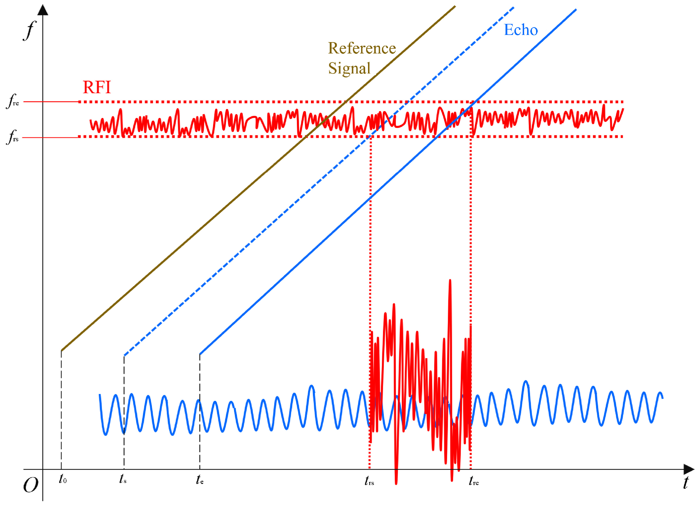
Here, t represents time; $K_r=B_w/T_r$ denotes the chirp rate. $W\left(t-{\displaystyle \frac{T_r}{2}},T_r\right)$ represents a time window centered at $T_r/2$ with a width of $T_r$. In an FMCW system, both the reference signal and the echo signal are delayed versions of the transmitted signal. Assume the delay of the reference signal is $t_0$, and the delay of the echo signal ranges from $t_s$ to $t_e$. A schematic diagram of the mixing process is shown in Figure 1.

As can be seen from the figure, the frequency difference between a given echo and the local oscillator delay is a constant at any given moment. Therefore, different range targets can be resolved via fast Fourier transform (FFT). The signal frequency corresponding to a delay of $t_s$ is:

$$F_s=K_r·\left(t_s-t_0\right)$$

(2)

Assuming the delay of the echo signal ranges from $t_s$ to $t_e$, the frequency range of the echo signal is:

$$\Delta F=F_e-F_s=K_r·\left(t_e-t_s\right)$$

(3)

Regarding RFI, as shown in Figure 1, interference is not continuously present. RFI affects the signal only when the interference frequency is close to the local oscillator signal frequency, and the resulting difference frequency falls between $F_e$ and $F_s$.

Assuming the RFI frequency ranges from $f_{rs}$ to $f_{re}$, with a bandwidth of $B_i$, and its time-domain duration is from $t_{rs}$ to $t_{re}$, then the following can be obtained:

$$f_{rs}=K_r·\left(t_{rs}-t_s\right)$$

(4)

$$f_{re}=K_r·\left(t_{re}-t_e\right)$$

(5)

After simplification, the time-domain duration of RFI can be obtained as:

$$T_{RFI}=t_{re}-t_{rs}={\displaystyle \frac{B_i}{K_r}}+t_e-t_s={\displaystyle \frac{B_i}{B_w}}·T_r+t_e-t_s$$

(6)

In general FMCW systems, to ensure the reliability of mixing, it is necessary to satisfy the condition $t_e-t_s\ll T_r$. For example, in an SAR system with a pulse width of 100 μs and a swath width of 2 km, assuming the bandwidth ratio $B_i/B_r$ is $5\%$, the duration of RFI is only 18.3 μs, which does not occupy the entire pulse width. This characteristic becomes even more pronounced in closer-range applications such as through-wall penetration.

3. Method

3.1. Modeling

Assuming the echo signal after mixing is $r\left(t\right)$, where t denotes the fast time, and $s\left(t\right)$ represents the RFI.

$$d\left(t\right)=r\left(t\right)+s\left(t\right)$$

(7)

Consider that $D\left(f,t\right)$ is the short-time Fourier transform (STFT) of $d\left(t\right)$. The following properties of $D\left(f,t\right)$ are considered in previous studies [17]:

• The signal of SOI occupies the entire signal bandwidth.
• The RFI occupies a narrow frequency band, which is commonly modeled as a sparse distribution.

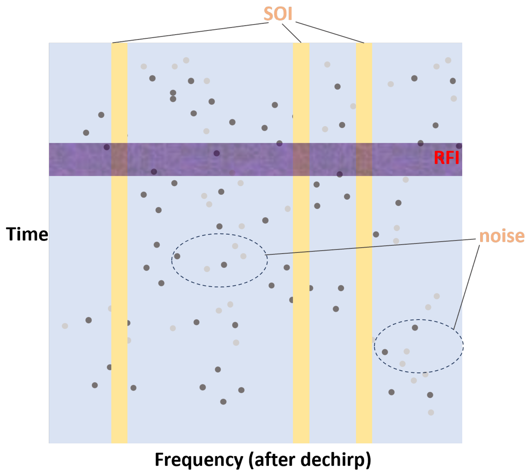
Based on these characteristics, $D\left(f,t\right)$ is represented as illustrated in Figure 2. It is observed that the SOI exhibits a low-rank structure and is continuously distributed along the time axis, which results from the inherent nature of the linear frequency-modulated signal. In contrast, RFI is sparsely distributed in the time–frequency domain. To exploit these properties for SOI extraction, let:

$$\mathbf{D}=\mathbf{L}+\mathbf{S}$$

(8)

where the time–frequency spectra of the original signal, SOI, and the RFI are denoted by $\mathbf{D}$, $\mathbf{L}$, and $\mathbf{S}$, respectively.

3.2. SOI Purification via Joint LRSR and TTV Constraints

To purify the SOI, the following optimization model is constructed:

$$\begin{array}{cc}& min{∥\mathbf{L}∥}_{*}+\lambda {∥\mathbf{S}∥}_1+\beta {∥\mathbf{L}∥}_{TTV}\hfill \\ & \begin{array}{cc}s.t.& \mathbf{D}=\mathbf{L}+\mathbf{S}\end{array}\hfill \end{array}$$

(9)

where the nuclear norm of $\mathbf{L}$, denoted by ${∥\mathbf{L}∥}_{*}=\sum {\sigma }_j\left(\mathbf{L}\right)$, represents the sum of the singular values of $\mathbf{L}$ and is employed to enforce the low-rank structure of the SOI. The ${\mathcal{l}}_1$-norm of $\mathbf{S}$, defined as ${∥\mathbf{S}∥}_1=\sum \left|{\mathbf{S}}_{ij}\right|$, corresponds to the sum of the absolute values of all elements and serves to promote the sparsity of the RFI. The total variation along the frequency axis, denoted as ${∥\mathbf{L}∥}_{TTV}={\parallel {\nabla }_T\mathbf{L}\parallel }_2^2$, is defined as the ${\mathcal{l}}_2$-norm of the variation in matrix $\mathbf{L}$ along the time dimension, characterizing the continuity of the SOI across different time. Let $l(m,n)$ denote the discrete STFT of $D\left(f,t\right)$, where m and n denote time and frequency samples, respectively. Thus,

$${∥\mathbf{L}∥}_{TTV}=\sum _{m,n}{\left[l(m+1,n)-l(m-1,n)\right]}^2$$

(10)

It should be emphasized that the low-rank characteristic helps effectively separate the SOI from RFI. However, when the hyperparameter $\mu$ of the low-rank model is improperly selected, residual RFI (RRFI) may be mistakenly classified as the SOI within the subspace, especially under low SINR conditions. This method leverages the discontinuity of RFI along the frequency axis and progressively suppresses RRFI through TTV regularization, thereby enhancing signal purification performance and parameter robustness.

The optimization problem formulated in Equation (9) is solved using the alternating ADMM. To facilitate the solution, an auxiliary variable $\mathbf{H}$ is introduced:

$$\begin{array}{cc}& min{∥\mathbf{H}∥}_{*}+\lambda {∥\mathbf{S}∥}_1+\beta {∥\mathbf{L}∥}_{TTV}\hfill \\ & \begin{array}{cc}s.t.& \begin{array}{cc}& \mathbf{D}=\mathbf{L}+\mathbf{S}\hfill \\ & \mathbf{H}=\mathbf{L}\hfill \end{array}\end{array}\hfill \end{array}$$

(11)

Based on Equation (11), the augmented Lagrangian function is constructed as follows:

$$\begin{array}{cc}& \mathcal{L}\left(\mathbf{S},\mathbf{I},\mathbf{H},{\mathbf{Y}}_1,{\mathbf{Y}}_2\right)={∥\mathbf{H}∥}_{*}+\lambda {∥\mathbf{S}∥}_1+\beta {∥\mathbf{L}∥}_{TTV}\hfill \\ & +{\displaystyle \frac{\mu }{2}}\left({∥\mathbf{D}-\mathbf{H}-\mathbf{S}∥}_F^2+{∥\mathbf{L}-\mathbf{H}∥}_F^2\right)\hfill \\ & +〈{\mathbf{Y}}_1,\mathbf{D}-\mathbf{L}-\mathbf{S}〉+〈{\mathbf{Y}}_2,\mathbf{L}-\mathbf{H}〉\hfill \end{array}$$

(12)

where $\lambda$, $\beta$, and $\mu$ denote the regularization parameters, while ${\mathbf{Y}}_1$ and ${\mathbf{Y}}_2$ correspond to the Lagrange multipliers. $〈·,·〉$ respresents the matrix inner product operation. For the objective function presented in Equation (12), the ADMM algorithm decomposes the original optimization problem into several subproblems with respect to different variables, thereby significantly reducing computational complexity. The iterative procedure of the ADMM algorithm is given as follows:

3.2.1. $\mathbf{H}$-Subproblem

By fixing all other variables, the subproblem associated with $\mathbf{H}$ can be formulated as follows:

$$\begin{array}{cc}\hfill {\mathbf{H}}_{k+1}=& \underset{\mathbf{H}}{argmin}{\displaystyle \frac{\mu }{2}}\left({∥\mathbf{D}-\mathbf{H}-{\mathbf{S}}_k∥}_F^2+{∥{\mathbf{L}}_k-\mathbf{H}∥}_F^2\right)\hfill \\ \hfill & +{∥\mathbf{H}∥}_{*}+〈{\mathbf{Y}}_{1,k},\mathbf{D}-\mathbf{H}-{\mathbf{S}}_k〉+〈{\mathbf{Y}}_{2,k},{\mathbf{L}}_k-\mathbf{H}〉\hfill \\ \hfill =& {∥\mathbf{H}∥}_{*}+\mu {∥\mathbf{H}-{\mathbf{A}}_k∥}_F^2\hfill \end{array}$$

(13)

where

$${\mathbf{A}}_k={\displaystyle \frac{1}{2}}\times (\mathbf{D}+{\mathbf{L}}_k-{\mathbf{S}}_k+{\mathbf{Y}}_{1,k}/\mu +{\mathbf{Y}}_{2,k}/\mu )$$

(14)

The optimization problem in Equation (13) can be solved using the singular value soft-thresholding algorithm [26]. Accordingly, ${\mathbf{H}}_{k+1}={\mathcal{D}}_{1/\mu }\left({\mathbf{A}}_k\right)$, where ${\mathcal{D}}_{\gamma }(·)$ denotes the soft-thresholding operator. Let the singular value decomposition (SVD) of a matrix $\mathbf{X}$ be $\mathbf{X}=\mathbf{U}\Sigma {\mathbf{V}}^H$, where $\Sigma =diag\left({\sigma }_i\right)$. Then,

$${\mathcal{D}}_{\gamma }\left(\mathbf{X}\right)=\mathbf{U}\mathrm{diag}\left(max({\sigma }_i-\gamma ,0)\right){\mathbf{V}}^H$$

(15)

3.2.2. $\mathbf{S}$-Subproblem

By fixing all other variables, the subproblem associated with $\mathbf{S}$ can be formulated as follows:

$$\begin{array}{cc}\hfill {\mathbf{S}}_{k+1}=& \underset{\mathbf{S}}{argmin}\lambda {∥\mathbf{S}∥}_1+{\displaystyle \frac{\mu }{2}}{∥\mathbf{D}-{\mathbf{H}}_k-\mathbf{S}∥}_F^2\hfill \\ \hfill & +〈{\mathbf{Y}}_{1,k},\mathbf{D}-{\mathbf{L}}_k-\mathbf{S}〉\hfill \\ \hfill =& \lambda {∥\mathbf{S}∥}_1+{\displaystyle \frac{\mu }{2}}{∥\mathbf{S}-{\mathbf{B}}_k∥}_F^2\hfill \end{array}$$

(16)

where

$${\mathbf{B}}_k=\mathbf{D}-{\mathbf{H}}_k+{\mathbf{Y}}_{1,k}/\mu$$

(17)

The optimization problem in Equation (16) can be efficiently solved using the soft-thresholding algorithm [26]. Accordingly, the update for $\mathbf{L}$ is given by ${\mathbf{L}}_{k+1}={\mathcal{G}}_{\lambda /\mu }\left({\mathbf{B}}_k\right)$, where

$${\mathcal{G}}_{\gamma }\left(\mathbf{X}\right)=max(\mathbf{X}-\gamma ,0)$$

(18)

3.2.3. $\mathbf{L}$-Subproblem

Similarly, the subproblem associated with $\mathbf{L}$ can be formulated as

$$\begin{array}{cc}\hfill {\mathbf{L}}_k& =\underset{\mathbf{L}}{argmin}\beta {∥\mathbf{L}∥}_{TTV}+{\displaystyle \frac{\mu }{2}}{∥\mathbf{L}-{\mathbf{H}}_k∥}_F^2+〈Y_2,\mathbf{L}-{\mathbf{H}}_k〉\hfill \\ \hfill & =\beta {∥\mathbf{L}∥}_{TTV}+{\displaystyle \frac{\mu }{2}}{∥\mathbf{L}-{\mathbf{C}}_k∥}_F^2\hfill \end{array}$$

(19)

where

$${\mathbf{C}}_k={\mathbf{H}}_k-{\mathbf{Y}}_{2,k}/\mu$$

(20)

This subproblem can be efficiently solved using a one-dimensional variant of the Fast Gradient-Based Algorithm (FGA) [27]. For convenience, the iterative process of FGA is simplified and encapsulated by the operator $\mathbf{tvs}(·)$, defined as

$${\mathbf{L}}_{k+1}=\mathbf{tvs}\left({\mathbf{C}}_k\right)$$

(21)

After a sufficient number of iterations, the denoised signal is recovered via the inverse short-time Fourier transform (ISTFT). The detailed procedure is summarized in Algorithm 1.

Algorithm 1: Time-varying RFI suppression approach via joint LRSR and TTV constraints in the time–frequency domain

3.3. RRFI Suppression Based on Sub-Band Coherence Factor

CF weighting is applied across sub-bands to effectively suppress RRFI. The underlying mechanism lies in the inherent difference in frequency-domain coherence between the SOI and RRFI: the SOI is typically broadband and maintains a stable phase relationship across channels in all sub-bands, thus exhibiting high inter-sub-band coherence, whereas RRFI is band-limited, appearing only in a limited number of sub-bands, which results in significantly reduced coherence. First, the signal $I\left(t\right)$ processed in the previous subsection is divided into multiple sub-bands, and the time-domain signal of the k-th sub-band can be expressed as:

$$I_k\left(t\right)=I\left(t\right)\ast H(f_k,B_w,t)$$

(22)

where $H(f_k,B_w,t)$ represents the time-domain response of a bandpass filter with center frequency $f_k$ and bandwidth $B_w$, and * denotes the convolution operation. The CF is defined as the power ratio between coherent and incoherent combinations:

$$CF\left(t\right)={\displaystyle \frac{{\left|{\sum }_{k=1}^K{I}_k\left(t\right)\right|}^2}{N{\sum }_{k=1}^K{\left|I_k\left(t\right)\right|}^2}}$$

(23)

The value closer to 1 indicates stronger consistency across sub-band signals, suggesting the signals originate from the target direction. Conversely, RRFI only appears in sub-bands where interference exists, resulting in poor inter-sub-band coherence and a smaller CF. Thus, a multiplicative operation can be applied to suppress RRFI.

$$I^{\prime }\left(t\right)=I\left(t\right)·C{F}^p\left(t\right)$$

(24)

The hyperparameter p controls the degree of weighting of the coherence factor: the higher the value of p, the stronger the interference suppression, although it also has some effect on weak target signals. Therefore, p is typically chosen between 0 and 1, and adjusting p allows for an acceptable balance between interference suppression and signal retention.

4. Results

4.1. Hyperparameter

It is well known that in sparse recovery problems, the selection of hyperparameters has a significant impact on the final performance. In the proposed method, the low-rank regularization coefficient $\mu$ can be determined from the singular value inflection point [28], i.e.,

$$\mu ={\displaystyle \frac{1}{2·\left|e\right|}}$$

(25)

$\lambda$ controls the extraction strength of sparse RFI: a larger $\lambda$ leads to sparser RFI, causing the model to attribute more variations in the data to anomalies, which may mistakenly remove useful details; a smaller $\lambda$ makes the model less sensitive to anomalies, potentially leaving residual noise. $\beta$ controls the smoothness of the low-rank SOI component: a larger $\beta$ results in smoother SOI, which can effectively suppress RFI but may oversmooth details and edges; a smaller $\beta$ preserves more structural details, but may lead to insufficient RFI suppression. In practical work, optimal parameter selection can be achieved by performing cross-validation on data from the first few pulses. A relaxed stopping threshold ($\xi =1\times {10}^{-4}$) was used, since subsequent CF-weighting processing provides additional suppression, even if RFI mitigation is not fully achieved in earlier stages. Section 4.2 and Section 4.3 have shown that even if the scenario changes to some extent later on, this method can still provide good suppression effects. It should be noted that when $\beta =0$, the LRSR-TTV method degenerates into the RPCA problem.

4.2. Numerical Simulation

The effectiveness of the LRSR-TTV method for moving target detection is evaluated through numerical simulations. To simulate the impact of interference, high-power narrowband noise is added to the echo data. The simulation parameters are summarized in

Table 1. Numerical simulation parameter.

Parameter	Symbol	Value
Signal power	$P_s$	−20 dBm
Interference power	$P_i$	−10 dBm/0 dBm
Noise power	$P_n$	25 dBm
Carrier frequency	$f_{cr}$	2 GHz
Signal bandwidth	$B_w$	2 GHz
Signal duration	$T_r$	100 μs
Interference bandwidth	$B_i$	100 MHz/50 MHz

.

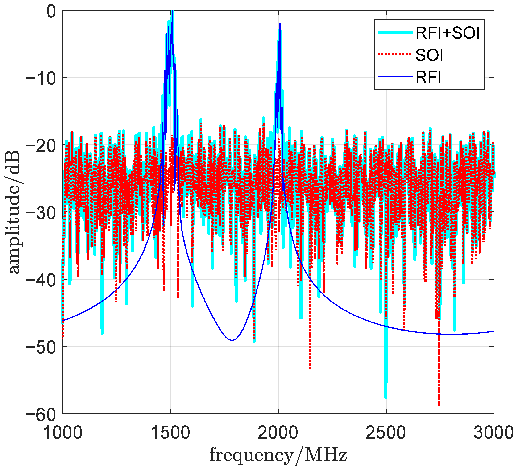
We captured actual RFI signals using a radar system, then cropped and frequency-stretched them to synthesize two RFI signals at different frequencies. With respect to the simulated target signal, these RFI signals were set at power levels of −10 dB and −20 dB, respectively. Figure 3 shows the spectrum at an SINR of −20 dB.

Figure 4 shows the RFI suppression results under a SINR of −10 dB. In this case, the RFI power is relatively low. Visually, both RPCA and the proposed LRSR-TTV method demonstrate good performance, while the primary effect of the CF weighting here is to reduce the scattered range sidelobes.

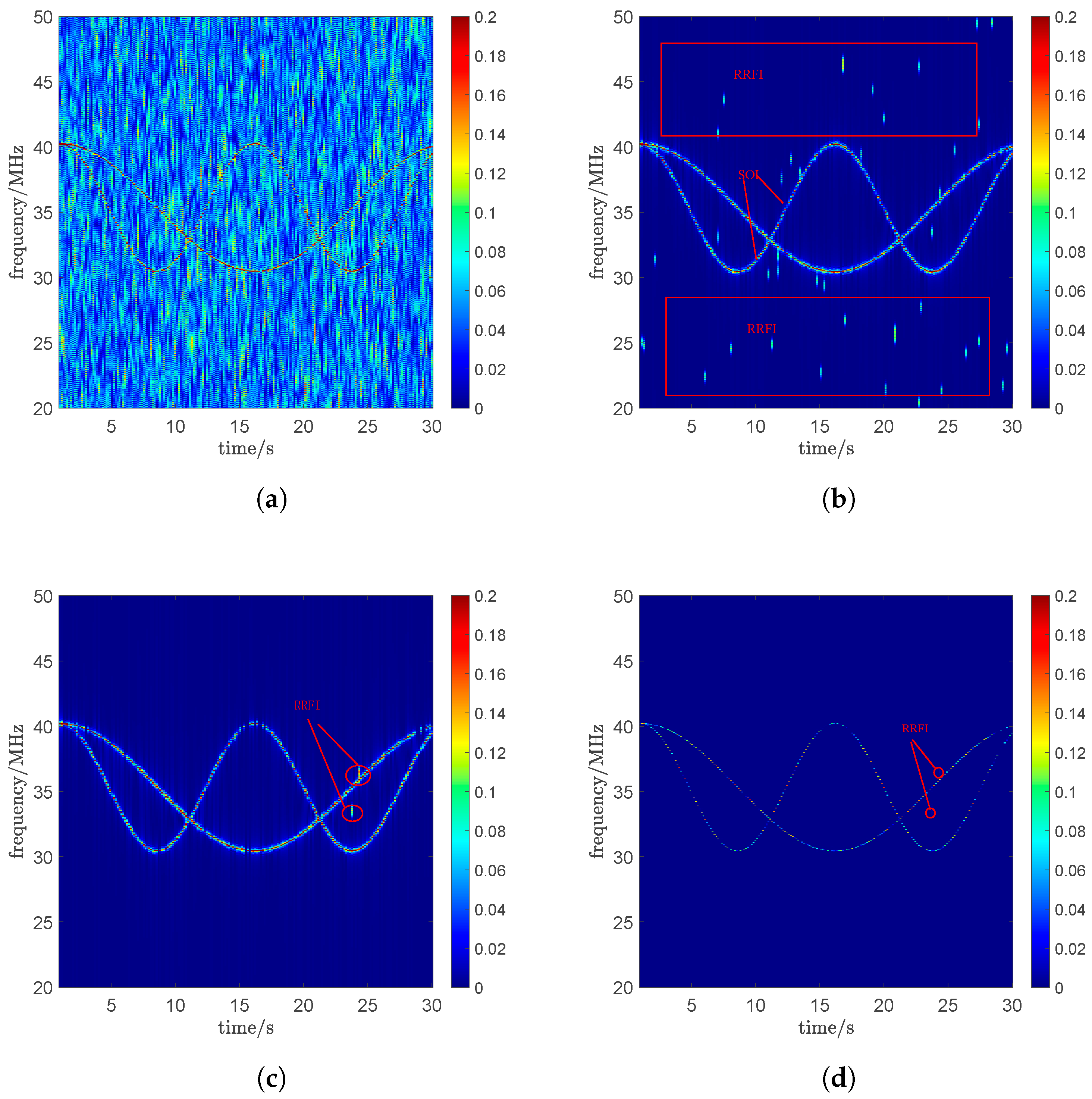
Figure 5 shows the RFI suppression results under a SINR of −20 dB. Due to the extremely high RFI power, the target signal is almost completely buried in the original result shown in Figure 5a. As shown in Figure 5b, RPCA significantly reduces RFI. However, a considerable amount of RRFI still remains. This is primarily because the severely low SINR causes the RFI subspace to intrude into the SOI subspace. Moreover, when solving the RPCA problem, the $l_0$-norm sparsity constraint on RFI is relaxed to an $l_1$-norm, resulting in model mismatch under high interference power. In contrast, the proposed method incorporates LRSR-TTV constraints to effectively mitigate the presence of RRFI, as shown in Figure 5c. This facilitates the progressive separation of the SOI and RFI subspaces during the optimization process and reduces the impact of model mismatch under low-SINR conditions. After CF weighting, RRFI is further suppressed as shown in Figure 5d.

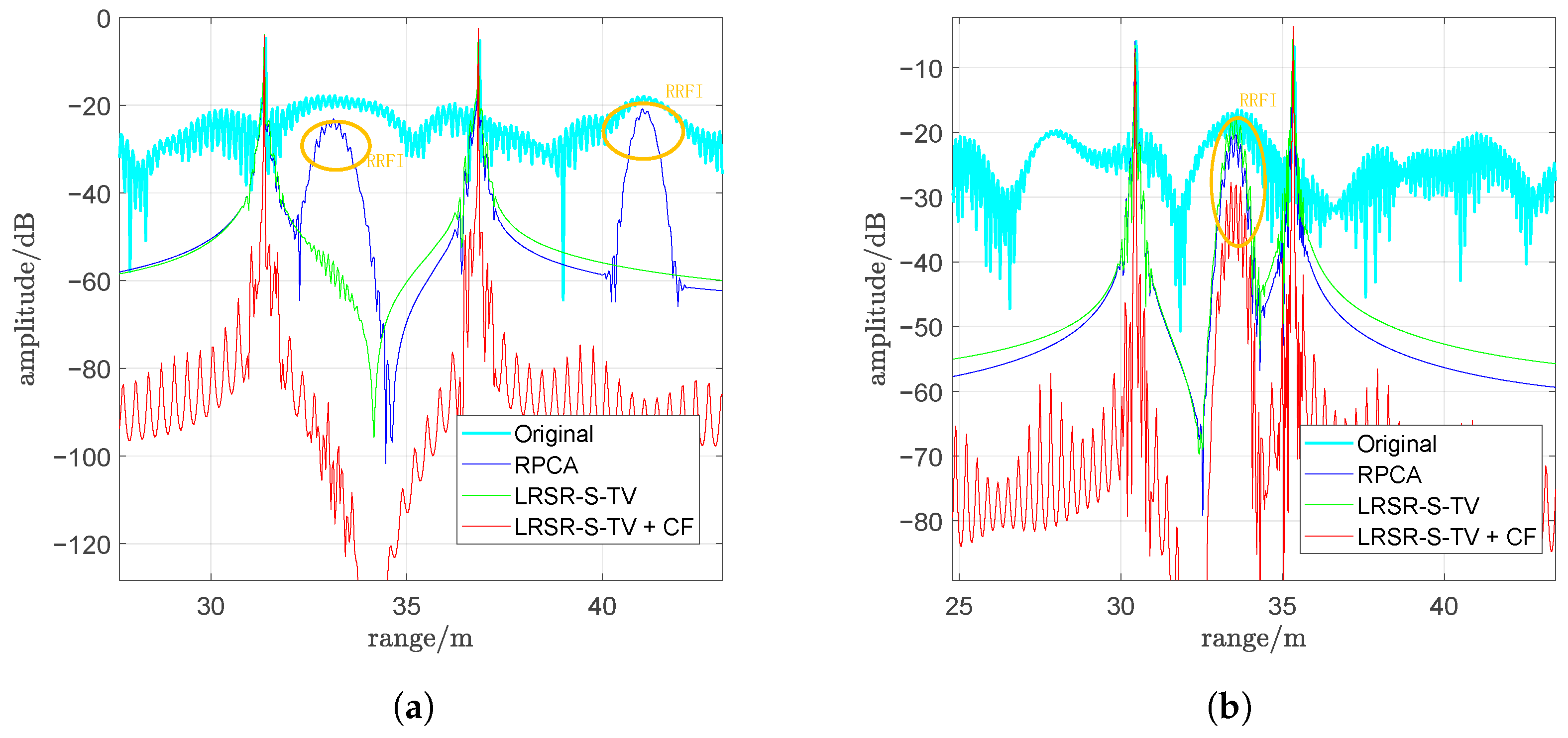
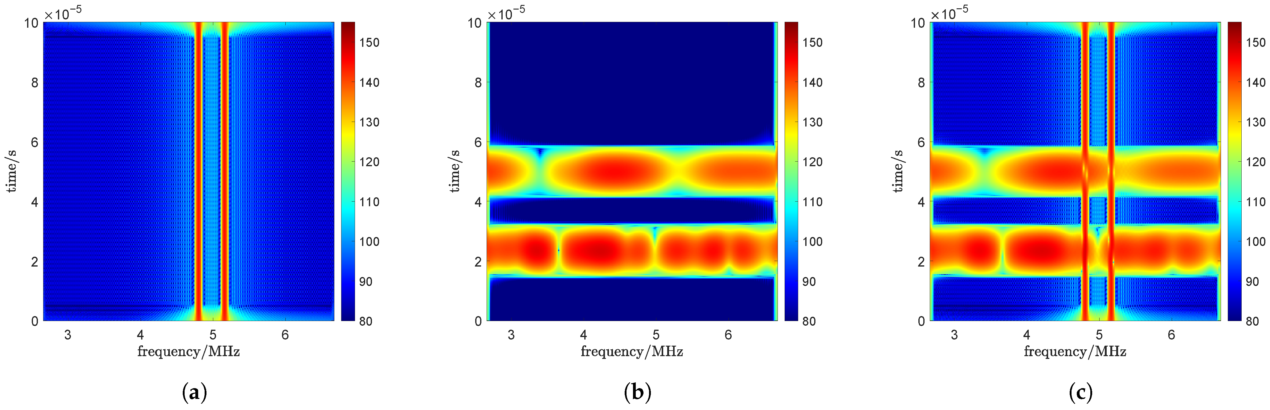
Figure 6 presents two one-dimensional profiles obtained by applying different methods to the data in Figure 5. In Figure 6a, significant residual RFI (RRFI) remains due to hyperparameter mismatch in the RPCA method. In contrast, the LRSR-TTV process leaves almost no residual RFI. Meanwhile, CF weighting substantially suppresses the sidelobes and enhances resolution. In Figure 6b, noticeable RRFI persists after both RPCA and LRSR-TTV processing, whereas CF weighting achieves approximately 8 dB of RRFI suppression and also improves resolution. Figure 7 shows the STFT results processed by different denoising methods, with the hyperparameters selected according to Equation (25). It can be observed that the RPCA method leaves substantial RRF in Figure 7b, whereas the proposed LRDR-TTV method only exhibits some RRFI at the target location in Figure 7c.

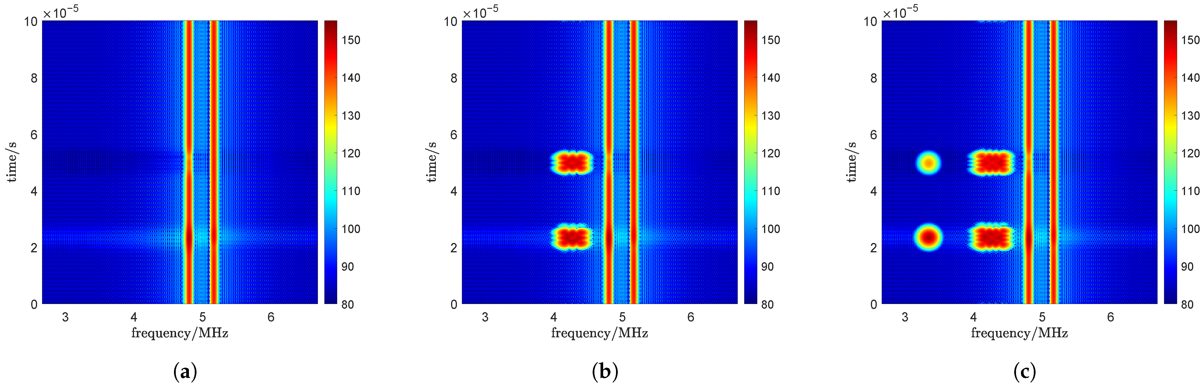
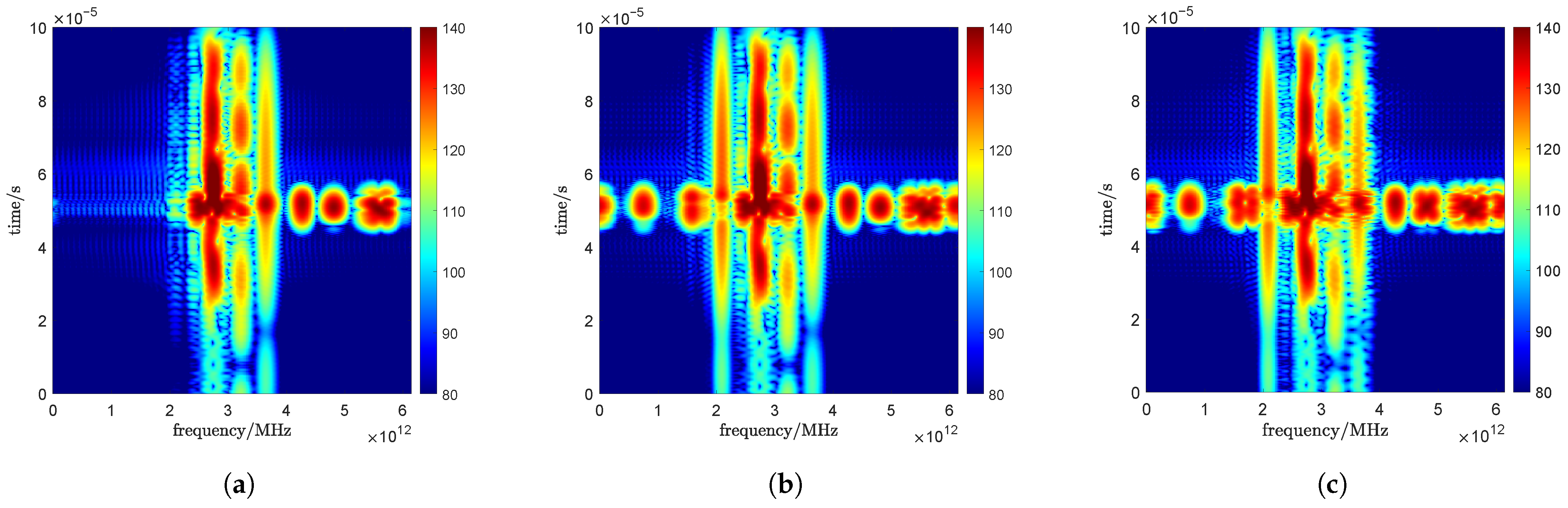
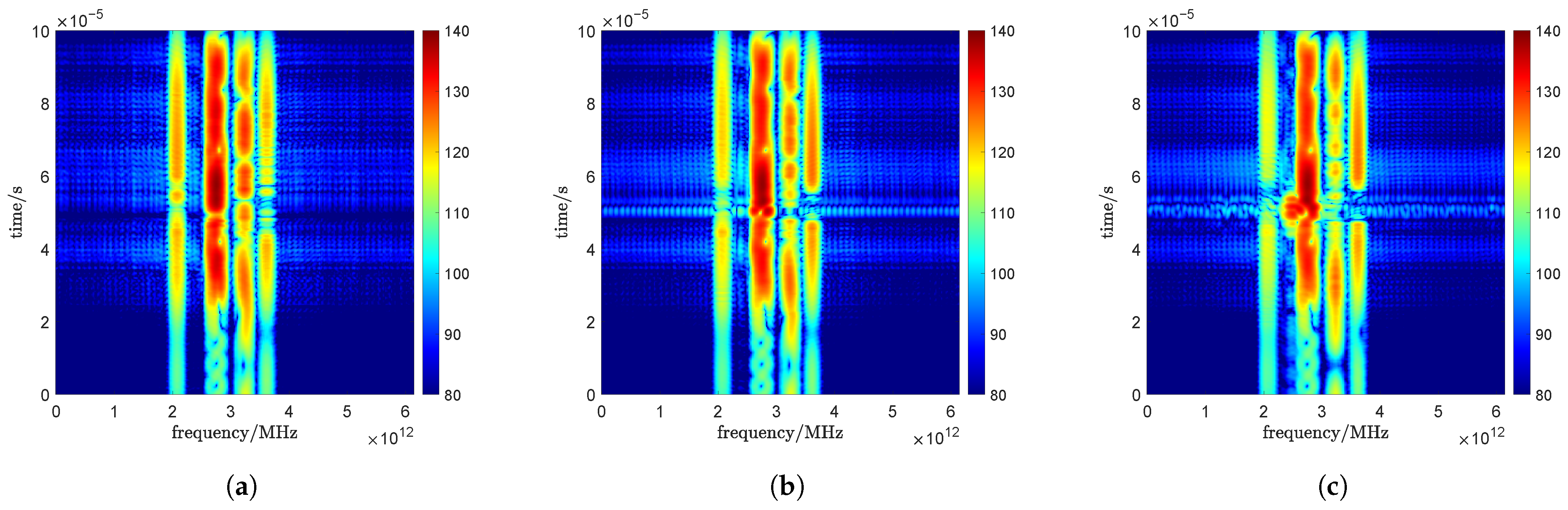
To demonstrate the fairness of hyperparameter selection, starting from the initial pulses, we tested multiple hyperparameters for the RPCA and LRSR-TTV methods around the elbow points of singular values. The corresponding STFT results are shown in Figure 8 and Figure 8 and the true value is shown in Figure 7. In this experiment, the second singular value was selected as the elbow point. The same situation also appears in Figure 8c. However, none of the tested elbow points produced satisfactory results: selecting a smaller singular value led to residual RFI that could not be eliminated, as also observed in Figure 8c. We also attempted to find a balance between $e_1$ and $e_2$, and as shown in Figure 8a, this parameter setting was able to achieve the desired effect.

Although fine-tuning parameters pulse by pulse might enable RPCA to match or even surpass the performance of the proposed method, this precisely highlights the advantage of LRSR-TTV; it can achieve commendable results with only rough cross-validation using the first few pulses, as shown in Figure 9.

Subsequently, the suppression effect of RFI under different SINR conditions was discussed. Image entropy is a commonly used evaluation criterion in radar detection [29,30], and it can be defined as

$$E=-\sum _{m=1}^M\sum _{n=1}^N{p}_{m,n}\log \left(p_{m,n}\right)$$

(26)

where the probability distribution function $p_{m,n}$ is

$$p_{m,n}={\displaystyle \frac{I\left(x_m,y_n\right)}{{\sum }_{m=1}^M{\sum }_{n=1}^{N}I\left(x_m,y_n\right)}}$$

(27)

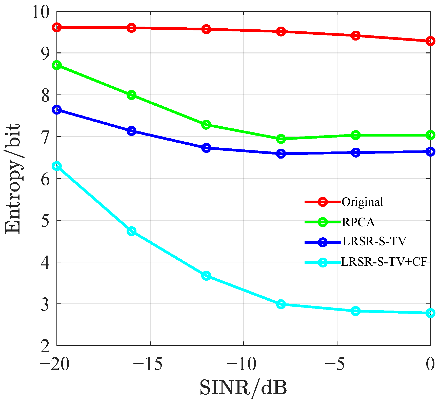
$I_{m,n}$ represents the one-dimensional range profile. m and n represent range and slow time samples, respectively. The entropy values of all the methods under varying SINR are statistically analyzed in Figure 10. It demonstrates that as the SINR increases, the image entropy gradually decreases, indicating progressive separation between the background region and target region. Moreover, the LRSR-TTV method consistently outperforms the RPCA approach, particularly under low SINR conditions where it still achieves certain clutter suppression effects. Besides mitigating RRFI, CF weighting further reduces sidelobe levels, resulting in lower image entropy.

We further compared the processing times of different spike signals under various methods, as shown in

Table 2. Statistical analysis of computational time.

Pulse Index	RPCA	LRSR-TTV
1	0.5028 s	0.5811 s
2	0.4870 s	0.5734 s
3	0.0648 s	0.5646 s
4	0.0629 s	0.5898 s
5	0.0706 s	0.6030 s

. Overall, the proposed method requires increased processing time. However, due to variations in the scenarios, the convergence time for each individual spike signal differs. The use of total variation regularization inevitably leads to improved results at the cost of a higher computational burden.

4.3. Real-World Data

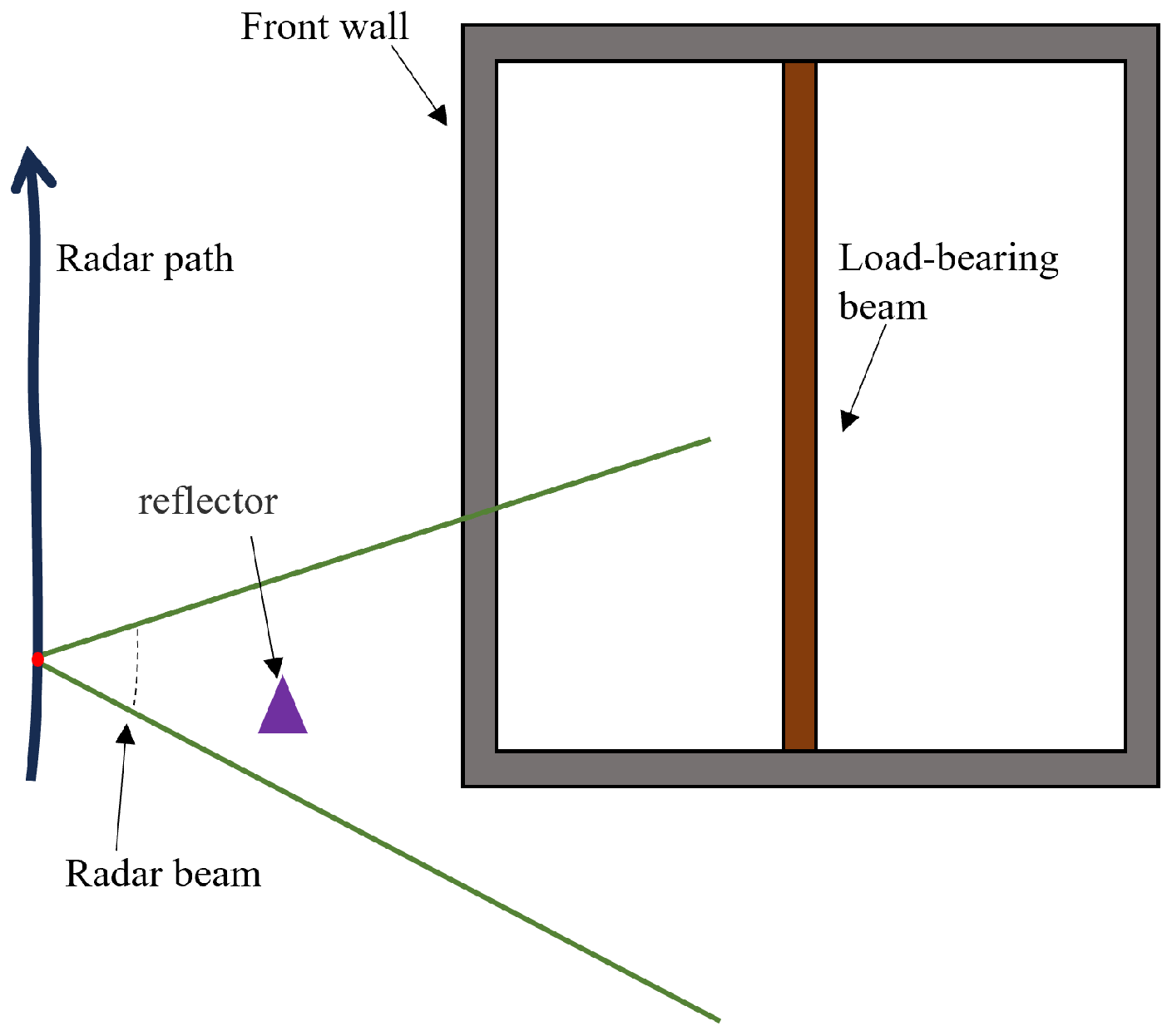
In this section, a practical UWB radar system is employed to demonstrate the effectiveness of the LRSR-TTV method. The experimental scenario is illustrated in the figure below, where the radar scans along a corridor of the building to detect the architectural layout of the room. The system parameters are summarized in

Table 3. Parameter of UWB radar.

Parameter	Symbol	Value
Transmission power	$P_t$	33 dBm
Noise figure	$N_F$	4 dB
Carrier frequency	$f_{cr}$	2 GHz
Signal bandwidth	$B_s$	2 GHz
Signal duration	$T_r$	100 μs
Antenna beamwidth	-	${45}^{\circ }\times {45}^{\circ }$
Polarization	-	HH

.

The experimental scenario is illustrated in Figure 11. In this setup, the radar scans the building along a linear trajectory to acquire echo signals. The received echoes contain reflections from the front wall, back wall, internal load-bearing beams, and external reflectors of the building.

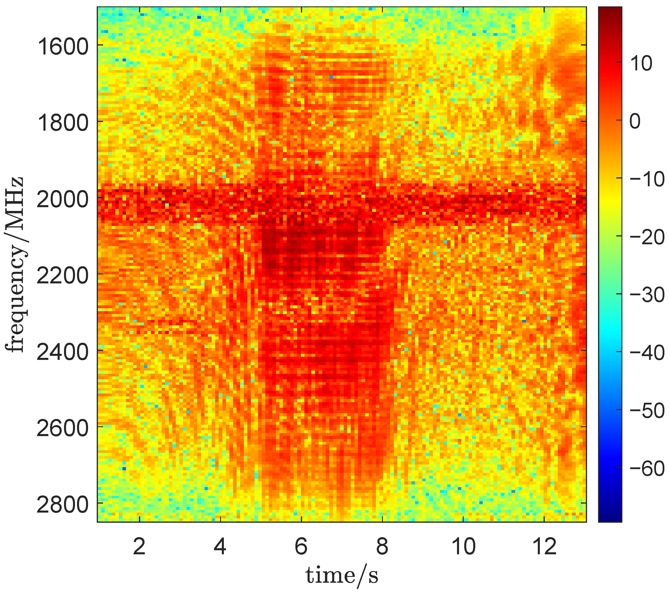
The spectrum of the acquired radar echoes is shown in Figure 12, where RFI from 2000 to 2100 MHz is clearly present. Due to variations in echo power with radar scanning, the SINR of the echoes also changes accordingly. For instance, when the radar scans walls, the SINR ranges between −8 and 0 dB, while in other areas, the SINR can reach as low as −15 dB.

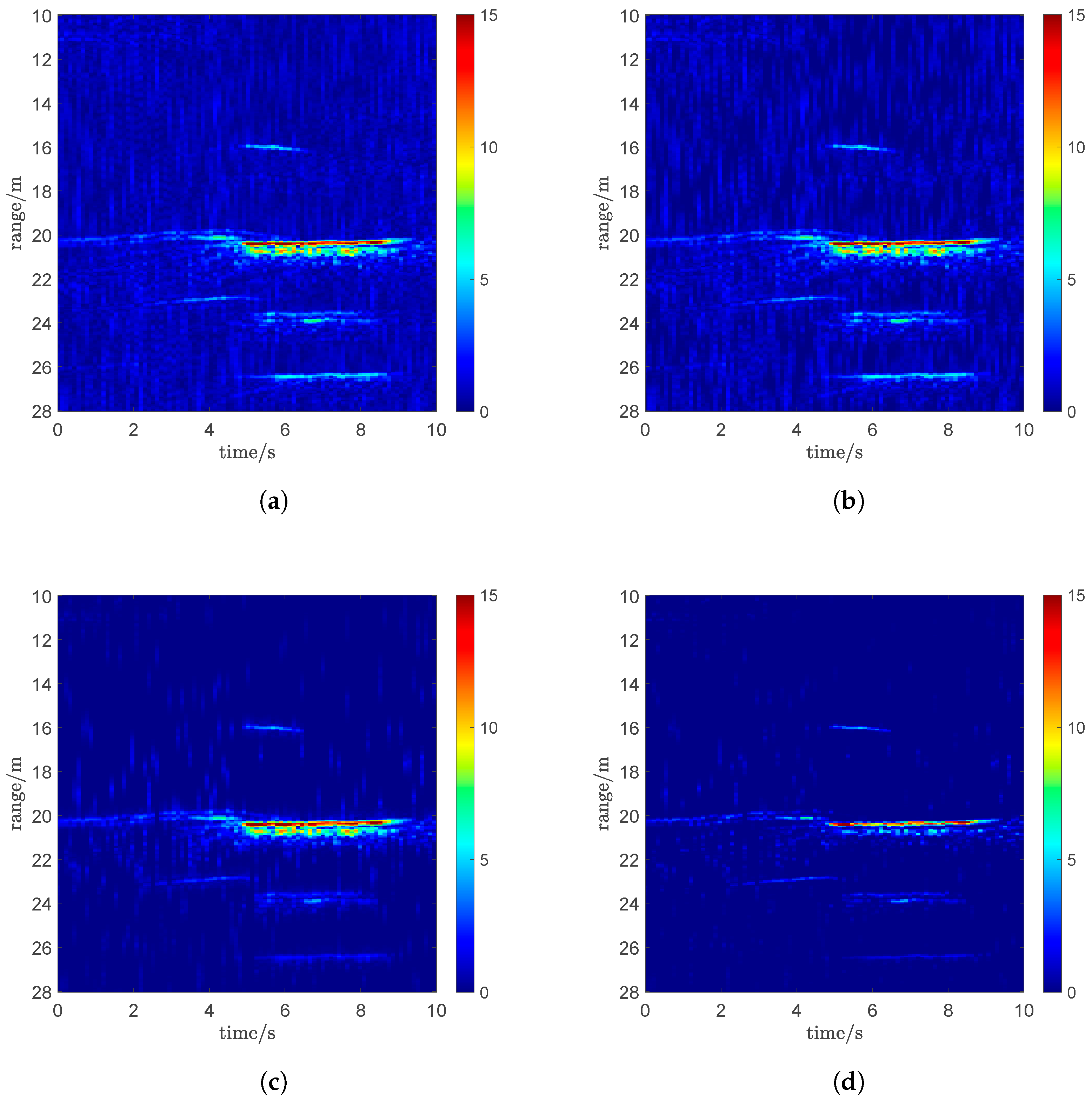
Figure 13 presents the one-dimensional range profiles obtained from radar scanning. Due to signal attenuation caused by the first wall, the reflections from the load-bearing wall and the back wall become extremely weak and are nearly buried in background noise induced by RFI, as shown in Figure 13a. To suppress the interference, both the time–frequency domain RPCA method and the LRSR-TTV approach are applied. As illustrated in Figure 13b, RPCA is capable of partially mitigating the interference. However, a significant amount of RRFI remains, making it difficult to discern the structures behind the wall. In contrast, the LRSR-TTV method effectively suppresses RRFI, allowing the structural details behind the wall to be clearly revealed, as shown in Figure 13c. After CF weighting, RRFI is further suppressed, resulting in a cleaner image background, as shown in Figure 13d.

Table 4. Image entropy with different methods.

Method	Original	RPCA	LRSR-TTV	LRSR-TTV and CF
Entropy/bit	15.42	14.30	10.09	5.37

summarizes the image entropy values obtained with different processing methods. The CF method after LRSR-TTV demonstrates the highest efficiency in entropy reduction, achieving the lowest entropy value (5.37 bits) and outperforming other methods. This indicates superior noise reduction capabilities, making it the most effective approach for minimizing RFI among the tested techniques.

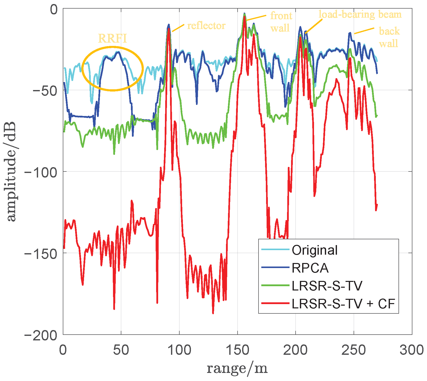
Figure 14 presents the one-dimensional range profiles after different processing methods at approximately 8 s. Although residual RRFI persists after RPCA processing, it is nearly eliminated by LRSR-TTV processing, while CF further narrows the main lobe. For weak targets, LRSR-TTV and CF cause some amplitude loss, but the overall SINR of the entire image is enhanced.

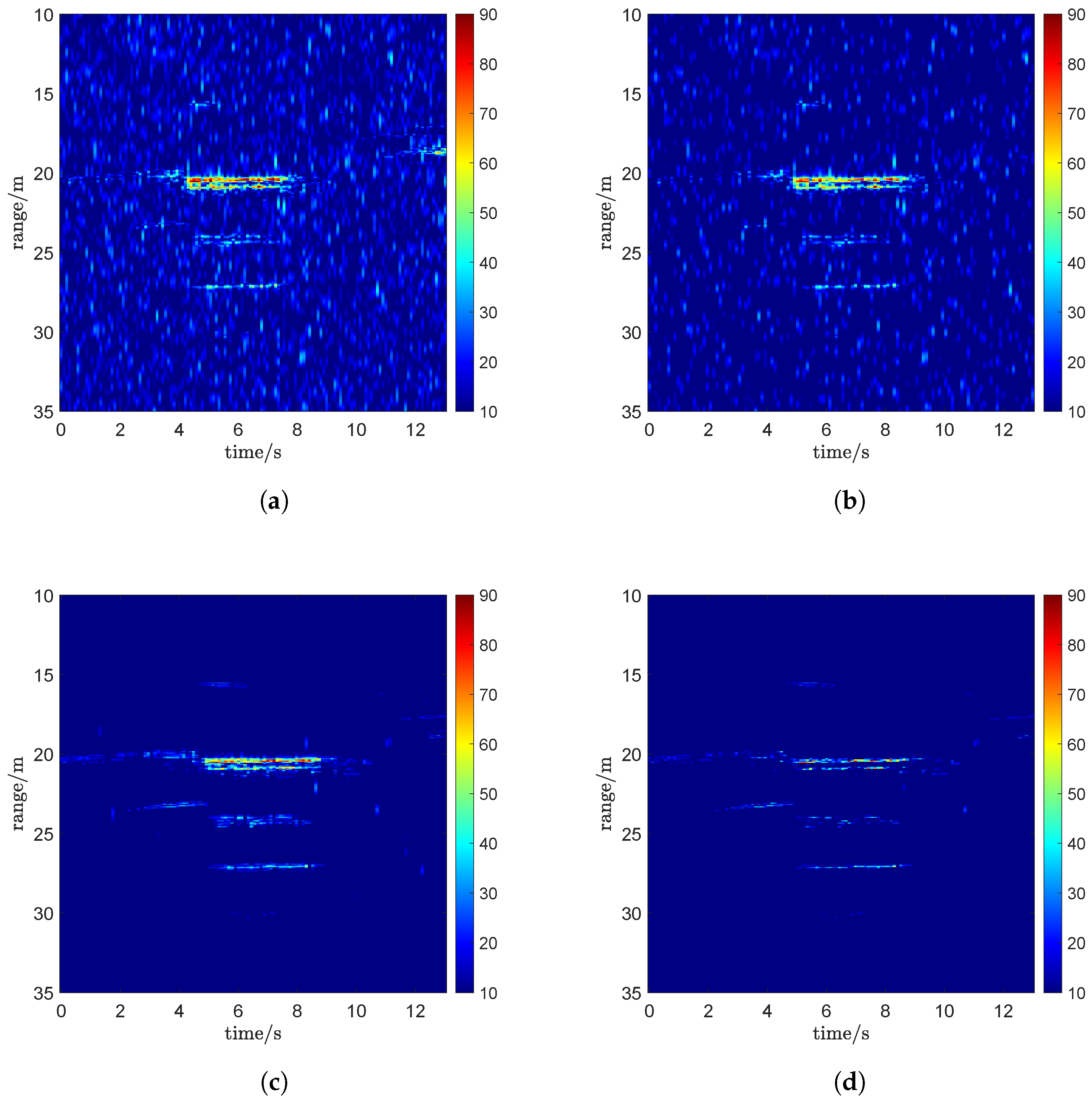
To further discuss the performance of the proposed method under low SINR conditions and to conduct a more in-depth analysis, a semi-physical simulation experiment was conducted in this paper. We simulated the SAR echoes based on the results in Figure 14, introducing radio frequency interference with an SINR of approximately −20 dB (for the wall region). The original image and the processed results are shown in Figure 15. Compared with the actual measured data, the performance of the several methods is comparable.

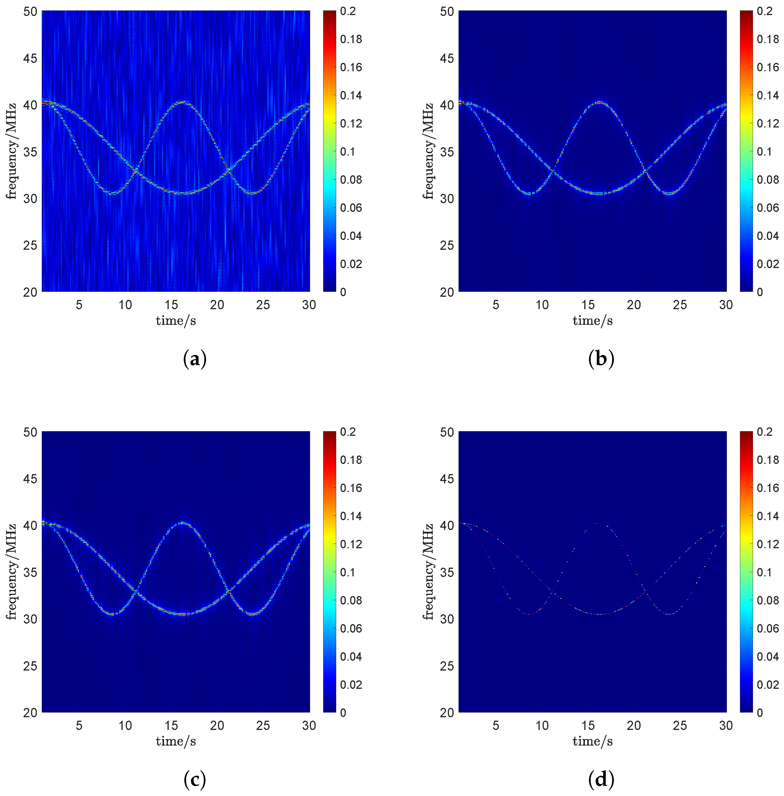
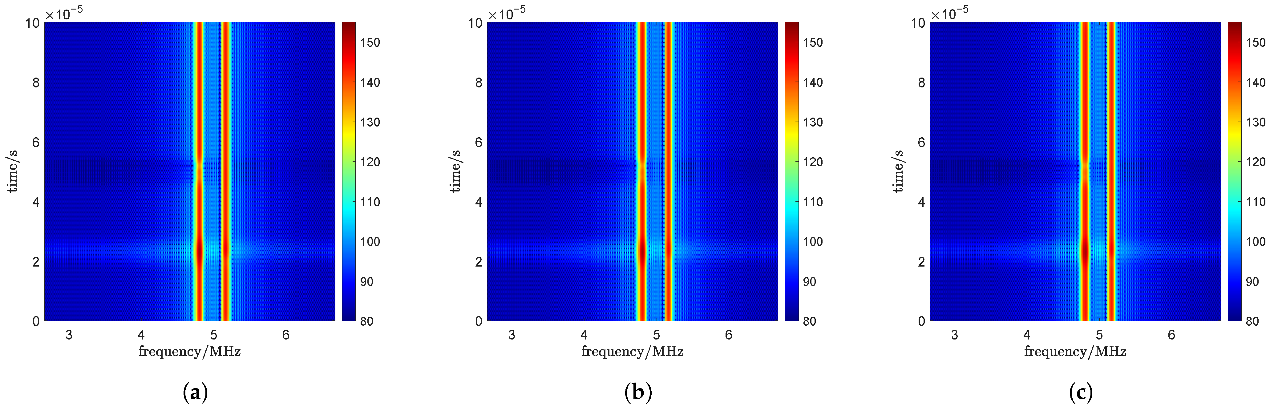
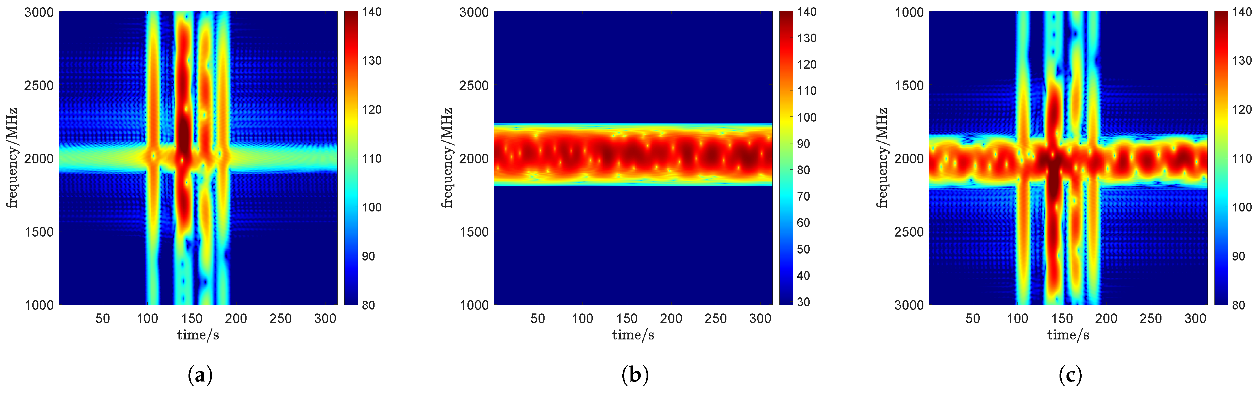
Figure 16 displays the time–frequency spectra of the SOI, the RFI, and their superposition around the 6-second mark, respectively. Since the echoes are generated based on interference-suppressed data, some RRFI remains in Figure 16a. However, its power is more than 20 dB lower than that of the signal, thus not affecting subsequent analysis. As is well known, LRSR-type methods are highly sensitive to the hyperparameter $\mu$. Therefore, Figure 17 and Figure 18 present results with different choices of the hyperparameter $\mu$. During the analysis, other hyperparameters were fixed via cross-validation and remained consistent across the compared methods. Among the selected parameters, the RPCA method exhibits target loss in Figure 16a, while Figure 16b,c show more RRFI. In contrast, the performance of the RPCA method is almost unaffected, showing only an acceptable level of loss within the interference frequency band.

5. Conclusions

This paper systematically validates the effectiveness and superiority of the proposed LRSR-TTV model for RFI suppression in UWB radar. Theoretical analysis and experimental results demonstrate that under the core challenge of low SINR, traditional RPCA methods suffer from significant residual interference due to the intrusion of the RFI subspace into the SOI subspace. In contrast, the proposed method successfully mitigates subspace confusion by incorporating LRSR-TTV constraints, leveraging the prior knowledge of SOI’s continuity along the frequency dimension in the time–frequency domain, thereby achieving cleaner signal separation. Further post-processing using sub-band CF weighting confirms its effectiveness as a supplementary measure for additional residual interference suppression. Both numerical simulations and real-world data experiments show that the proposed method maintains excellent performance even under extremely low SINR conditions, significantly outperforming existing RPCA-based approaches. The lower image entropy values obtained demonstrate its potential for enhancing imaging quality.

References

1. Cardoni, A.; Cimellaro, G.P. Development and Validation of a UAV-Based Ultra-Wideband Localization System for Indoor Search and Rescue. Remote Sens. Appl. Soc. Environ. 2026, 41, 101884. [Google Scholar] [CrossRef]
2. Wang, J.; Chen, L.Y.; Liang, X.D.; Ding, C.B.; Li, K. Implementation of the OFDM chirp waveform on MIMO SAR systems. IEEE Trans. Geosci. Remote Sens. 2015, 53, 5218–5228. [Google Scholar] [CrossRef]
3. Wang, J.; Liang, X.D.; Chen, L.Y.; Li, Y.L. Waveform designs for joint wireless communication and radar sensing: Pitfalls and opportunities. IEEE Internet Things J. 2023, 10, 15252–15265. [Google Scholar] [CrossRef]
4. Zhang, C.; Gao, G.; Zhang, L.; Chen, C.; Gao, S.; Yao, L.; Bai, Q.; Gou, S. A novel full-polarization SAR image ship detector based on scattering mechanisms and wave polarization anisotropy. ISPRS J. Photogramm. Remote Sens. 2022, 190, 129–143. [Google Scholar] [CrossRef]
5. Li, H.L.; Chen, S.W. General Polarimetric Correlation Pattern: A Visualization and Characterization Tool for Target Joint-Domain Scattering Mechanisms Investigation. IEEE Trans. Geosci. Remote Sens. 2025, 64, 5200417. [Google Scholar] [CrossRef]
6. Li, H.L.; Chen, S.W. Polyhedral corner reflectors multi-domain joint characterization with fully polarimetric radar. IEEE Trans. Antennas Propag. 2025, 17, 10679–10693. [Google Scholar] [CrossRef]
7. Li, N.; Chen, J.; Guo, S.; Hao, X.; Qiu, C.; Cui, G.; Yang, X. Building Layout Tomographic Imaging Based on MIMO-UWB Radar. IEEE Trans. Geosci. Remote Sens. 2024, 62, 5108713. [Google Scholar] [CrossRef]
8. Xu, X.; Li, W.; Tang, H.; Chen, L.; Zhang, C.; Jiang, T.; Liu, J.; Liang, X. Bayesian Time-Domain Ringing Suppression Approach in Impulse Ultrawideband Synthetic Aperture Radar. Remote Sens. 2025, 17, 1455. [Google Scholar] [CrossRef]
9. Yang, X.; Gao, W.; Qu, X.; Ma, Z.; Zhang, H. Through-the-Wall Radar Human Activity Micro-Doppler Signature Representation Method Based on Joint Boulic-Sinusoidal Pendulum Model. IEEE Trans. Microw. Theory Tech. 2025, 73, 1248–1263. [Google Scholar] [CrossRef]
10. Li, W.; Chen, L.; Tang, H.; Zhang, F.; Xu, X.; Zhang, C.; Liu, J.; Yu, J. Error Analysis and Correction Method of Through-Wall Tomographic SAR. IEEE Trans. Aerosp. Electron. Syst. 2025. [Google Scholar] [CrossRef]
11. Jin, T.; Zhou, Z.; Song, Q.; Chang, W. UWB SAR RFI suppression based on region of support in 2-D wavenumber domain. J. Electron. 2007, 24, 503–508. [Google Scholar] [CrossRef]
12. Li, Y.L.; Li, X.Y.; Zhou, Z.M. Side-Lobe Reduction for Radio Frequency Interference Suppression via Clipping of Strong Scatterers. IEEE Geosci. Remote Sens. Lett. 2016, 13, 1178–1182. [Google Scholar] [CrossRef]
13. Liu, Z.; Liao, G.; Yang, Z. Time Variant RFI Suppression for SAR Using Iterative Adaptive Approach. IEEE Geosci. Remote Sens. Lett. 2013, 10, 1424–1428. [Google Scholar] [CrossRef]
14. Tao, M.; Zhou, F.; Liu, J.; Liu, Y.; Zhang, Z.; Bao, Z. Narrow-Band Interference Mitigation for SAR Using Independent Subspace Analysis. IEEE Trans. Geosci. Remote Sens. 2014, 52, 5289–5301. [Google Scholar] [CrossRef]
15. Nguyen, L.H.; Tran, T.D. A comprehensive performance comparison of RFI mitigation techniques for UWB radar signals. In Proceedings of the 2017 IEEE International Conference on Acoustics, Speech and Signal Processing (ICASSP), New Orleans, LA, USA, 5–9 March 2017; pp. 3086–3090. [Google Scholar] [CrossRef]
16. Song, Y.; Hu, J.; Jin, T.; Li, Z.; Chu, N.; Zhou, Z. Estimation and Mitigation of Time-Variant RFI Based on Iterative Dual Sparse Recovery in Ultra-Wide Band Through-Wall Radar. IEEE J. Sel. Top. Appl. Earth Obs. Remote Sens. 2019, 12, 3398–3411. [Google Scholar] [CrossRef]
17. Lyu, Q.; Han, B.; Li, G.; Sun, W.; Pan, Z.; Hong, W.; Hu, Y. SAR Interference Suppression Algorithm Based on Low-Rank and Sparse Matrix Decomposition in Time–Frequency Domain. IEEE Geosci. Remote Sens. Lett. 2022, 19, 4008305. [Google Scholar] [CrossRef]
18. Nguyen, L.H.; Tran, T.D. RFI-radar signal separation via simultaneous low-rank and sparse recovery. In Proceedings of the 2016 IEEE Radar Conference (RadarConf), Philadelphia, PA, USA, 2–6 May 2016; pp. 1–5. [Google Scholar] [CrossRef]
19. Liu, H.; Li, D. RFI Suppression Based on Sparse Frequency Estimation for SAR Imaging. IEEE Geosci. Remote Sens. Lett. 2016, 13, 63–67. [Google Scholar] [CrossRef]
20. Nguyen, L.H.; Tran, T.D. Efficient and Robust RFI Extraction Via Sparse Recovery. IEEE J. Sel. Top. Appl. Earth Obs. Remote Sens. 2016, 9, 2104–2117. [Google Scholar] [CrossRef]
21. Nguyen, L.H.; Tran, T.D. Separation of radio-frequency interference from SAR signals via dictionary learning. In Proceedings of the 2018 IEEE Radar Conference (RadarConf18), Oklahoma City, OK, USA, 23–27 April 2018; pp. 0908–0913. [Google Scholar] [CrossRef]
22. Huang, Y.; Liao, G.; Li, J.; Xu, J. Narrowband RFI Suppression for SAR System via Fast Implementation of Joint Sparsity and Low-Rank Property. IEEE Trans. Geosci. Remote Sens. 2018, 56, 2748–2761. [Google Scholar] [CrossRef]
23. Huang, Y.; Liao, G.; Zhang, L.; Xiang, Y.; Li, J.; Nehorai, A. Efficient Narrowband RFI Mitigation Algorithms for SAR Systems With Reweighted Tensor Structures. IEEE Trans. Geosci. Remote Sens. 2019, 57, 9396–9409. [Google Scholar] [CrossRef]
24. Li, S.; Amin, M.; An, Q.; Zhao, G.; Sun, H. 2-D Coherence Factor for Sidelobe and Ghost Suppressions in Radar Imaging. IEEE Trans. Antennas Propag. 2019, 68, 1204–1209. [Google Scholar] [CrossRef]
25. Yang, X.; Meng, H.; Ma, Z.; Qu, X.; Gao, W.; Zhao, Y. Azimuth Sidelobe Suppression Method for Through-the-Wall Radar Based on Phase Nonuniform Quantized Coherence Factor. IEEE Trans. Aerosp. Electron. Syst. 2025, 61, 7140–7152. [Google Scholar] [CrossRef]
26. Cai, J.F.; Candès, E.J.; Shen, Z. A Singular Value Thresholding Algorithm for Matrix Completion. SIAM J. Optim. 2010, 20, 1956–1982. [Google Scholar] [CrossRef]
27. Beck, A.; Teboulle, M. Fast Gradient-Based Algorithms for Constrained Total Variation Image Denoising and Deblurring Problems. IEEE Trans. Image Process. 2009, 18, 2419–2434. [Google Scholar] [CrossRef]
28. Falini, A. A review on the selection criteria for the truncated SVD in Data Science applications. J. Comput. Math. Data Sci. 2022, 5, 100064. [Google Scholar] [CrossRef]
29. Zhang, S.; Liu, Y.; Li, X. Fast Entropy Minimization Based Autofocusing Technique for ISAR Imaging. IEEE Trans. Signal Process. 2015, 63, 3425–3434. [Google Scholar] [CrossRef]
30. Long, T.; Lu, Z.; Ding, Z.; Liu, L. A DBS Doppler Centroid Estimation Algorithm Based on Entropy Minimization. IEEE Trans. Geosci. Remote Sens. 2011, 49, 3703–3712. [Google Scholar] [CrossRef]
Figure 1. Dechirping and RFI analysis in FMCW radar.
Electronics 15 00735 g001
Figure 2. Schematic diagram of time–frequency spectrum of FMCW signal.
Electronics 15 00735 g002
Figure 3. Signal spectrum in the presence of interference (SINR = −20 dB).
Electronics 15 00735 g003
Figure 4. Numerical simulation results (SINR = −10 dB). (a) Original; (b) RPCA; (c) LRSR-TTV; (d) LRSR-TTV and CF.
Electronics 15 00735 g004
Figure 5. Numerical simulation results (SINR = −20 dB). (a) Original; (b) RPCA; (c) LRSR-TTV; (d) LRSR-TTV and CF.
Electronics 15 00735 g005
Figure 6. PSF of simulation results (SINR = −20 dB). Pulse at approximately (a) 26 s and (b) 43 s.
Electronics 15 00735 g006
Figure 7. The STFT result of (a) ROI, (b) SOI, and (c) ROI + SOI.
Electronics 15 00735 g007
Figure 8. The result of STFT after RPCA in different hyperparameters. (a) μ = 1 e 1 + 1 e 2 ; (c) μ = 1 2 · e 1 ; (b) μ = 1 2 · e 2 , where e i denotes the i-th singular value.
Electronics 15 00735 g008
Figure 9. The result of STFT after LRSR-TTV in different hyperparameters. (a) μ = 1 e 1 + 1 e 2 ; (c) μ = 1 2 · e 1 ; (b) μ = 1 2 · e 2 .
Electronics 15 00735 g009
Figure 10. SINR-dependent changes in image entropy following RFI suppression.
Electronics 15 00735 g010
Figure 11. Experiment scene.
Electronics 15 00735 g011
Figure 12. Spectrum of the radar scanning echo.
Electronics 15 00735 g012
Figure 13. RFI suppression results of real-world data. (a) Original; (b) RPCA; (c) LRSR-TTV; (d) LRSR-TTV and CF.
Electronics 15 00735 g013
Figure 14. PSF of real-world supression results.
Electronics 15 00735 g014
Figure 15. Semi-physical simulation results (SINR = −20 dB). (a) Original; (b) RPCA; (c) LRSR-TTV; (d) LRSR-TTV and CF.
Electronics 15 00735 g015
Figure 16. The STFT result (semi-physical simulation) of (a) ROI, (b) SOI, and (c) ROI + SOI.
Electronics 15 00735 g016
Figure 17. The result of STFT after RPCA in different hyperparameters (semi-physical simulation). (a) μ = 1 2 · e 9 ; (b) μ = 1 2 · e 15 ; (c) μ = 1 2 · e 20 .
Electronics 15 00735 g017
Figure 18. The result of STFT after LRSR-TTV in different hyperparameters (semi-physical simulation). (a) μ = 1 2 · e 9 ; (b) μ = 1 2 · e 15 ; (c) μ = 1 2 · e 20 .
Electronics 15 00735 g018