A Variable Frequency Agricultural Sensing Method Based on Deep Prediction

Abstract

To address the challenges of low data validity and limited energy efficiency in agricultural IoT, we propose a deep predictive agricultural variable-frequency sensing method. First, we construct a hybrid prediction model, denoted as SVMD-TCN-R-GRU-T (STRGT). This model integrates successive variational mode decomposition (SVMD) with an optimized TCN-GRU architecture, thereby improving prediction accuracy. Building on this framework, we design a frequency conversion sampling method under dual detection analysis (FCSDDA). This approach employs wavelet transform to determine the minimum sampling rate and incorporates dynamic time warping evaluate data variation. The dual detection mechanism enables real-time adjustment of sensor acquisition frequency. Experimental results demonstrate that the proposed model significantly outperforms conventional models in terms of RMSE, MAE, and MAPE. When the STRGT outputs are applied as inputs to the FCSDDA algorithm, the system achieved optimal improvements in energy efficiency improvement rate (84.61%) and data value density (0.3368), exceeding the performance of other prediction model variants. These findings confirm that prediction accuracy directly influences adaptive sensing performance. This indicates that the method can effectively achieve dual optimization of energy saving and data validity in testing scenarios. In the future, more agricultural sensing scenarios can be validated.

1. Introduction

Against the backdrop of accelerating global urbanization and a rapidly aging population, agriculture is confronted with increasingly severe food security challenges [1,2]. To address these issues, data-driven smart agriculture [3] has emerged as a promising production model. By enhancing production efficiency, optimizing resource utilization, and reducing environmental impact, smart agriculture is widely recognized as a key pathway to ensuring food security. At its core, smart agriculture depends on large volumes of accurate agricultural data [4], encompassing environmental variables (e.g., climate and soil moisture) as well as diverse indicators across the crop growth cycle. These data provide the foundation for the broad application of agricultural big data analytics and artificial intelligence.

Data collection technology, with the agricultural internet of things (IoT) at its core, enables real-time monitoring of environmental parameters such as soil moisture, temperature, and light through sensor networks deployed in farmland. The collected data are transmitted to edge nodes, base stations, or cloud servers for processing. This low-power, cost-effective, and self-organizing network architecture provides a reliable data foundation for smart agriculture, thereby making agricultural production more precise and intelligent. Nevertheless, current agricultural IoT systems face several challenges, particularly limited node energy, high energy consumption, and the generation of large volumes of invalid data, all of which significantly hinder overall system performance.

In practical applications, much of the data collected through continuous agricultural sensing is irrelevant or redundant, often exhibiting high similarity across time and space [5]. These redundant data on the one hand occupy valuable resources and cause unnecessary system overhead [6]. On the other hand, a significant amount of time and effort in agricultural IoT is wasted on cleaning and discovering useful data. To address these issues, researchers have proposed various data collection strategies to enhance the efficiency of agricultural IoT systems. Common approaches include: (1) sensor duty-cycle allocation, which reduces energy consumption and mitigates redundant data generation by extending sensor sleep periods and limiting active sensing time; and (2) sensor selection sensing, which streamlines data acquisition by activating only a subset of sensors, thereby minimizing unnecessary monitoring and lowering energy usage. Although these methods have achieved notable results in practice, prediction-based variable-frequency sensing has received limited attention and remains insufficiently explored in the context of agricultural IoT.

The core concept of variable-frequency sensing is to adjust the data collection interval (sampling frequency) of sensor nodes based on the dynamic variations of the monitored physical variables. This approach minimizes invalid measurements, extends the low-power state of sensors, and reduces unnecessary energy consumption and redundant data collection, thereby enhancing overall system efficiency. However, this method is not sufficient to monitor physical phenomena that exhibit rapid changes. In this case, shortening the sampling interval is crucial to ensure that these short-term changes are accurately captured.

An effective strategy to address this limitation is to integrate variable-frequency sensing with data prediction. By employing predictive models to estimate future sensor readings, the system can determine either the appropriate timing for the next data collection and transmission or the optimal number of samples to be collected within a given period. In this way, variable-frequency sampling can anticipate data trends, minimize the number of samples required in each interval, and still capture essential information [7]. This not only reduces energy consumption without compromising data integrity but also enhances the overall effectiveness of data collection and the utilization efficiency of data value.

In the past, only the traditional prediction method and frequency conversion sampling were used. Gupta et al. [8] applied a variation of the exponential double smoothing (EDS) prediction model [9] together with the exponentially weighted moving average [10] to dynamically regulate sensor sampling intervals in air pollution monitoring. Building on this idea, Monteiro et al. [11] introduced a variable-frequency sampling method that integrates the transmission control protocol (TCP) cubic binary increase congestion control (CUBIC) algorithm with an EDS model, achieving improved energy savings. Cecchinel et al. [12] employed a machine learning approach that combined polynomial regression with variable-frequency sampling to optimize sensor configurations and extend battery life. Their method successfully prolonged the operational lifespan of temperature sensors from months to years while maintaining sufficient data quality, though they noted that performance was highly dependent on prediction accuracy. Hussein et al. [13] proposed an autoregressive prediction approach in which predicted values for the next cycle were compared with new sensor readings; data collection proceeded only when significant differences were detected. Halla et al. [14] utilized an LSTM-based prediction model, where the data collection frequency of sensor nodes was adjusted according to prediction error. Their model was updated using a set of tracking parameters, trained on the cluster head (CH) node, and executed directly on the sensor node.

Although numerous variable-frequency sensing methods have been proposed to reduce sensor node activity in the IoT, few have been applied specifically to agriculture, and even fewer deployed on edge nodes. In particular, prediction-based frequency sensing strategies have not fully leveraged deep prediction models. The effectiveness of such strategies in terms of energy savings and redundant data reduction is highly dependent on prediction accuracy [15,16].

Therefore, this paper proposes a variable-frequency agricultural sensing approach based on deep prediction. Deployed at the edge, the method integrates our deep prediction model with the frequency conversion sampling method under dual detection analysis (FCSDDA). By dynamically adjusting the sensing frequency of sensor nodes, the system increases data collection during critical periods and reduces it during less significant intervals. This adaptive mechanism enhances the data value density of sensing while simultaneously lowering overall system energy consumption.

2. Materials and Methods

2.1. Deep Prediction Model

2.1.1. SVMD

Variational mode decomposition (VMD) is a data-driven signal decomposition technique designed to overcome the modal aliasing problem of empirical mode decomposition (EMD). It decomposes the original data into k intrinsic mode functions (IMFs) to enable multi-scale analysis. However, VMD suffers from several limitations, including sensitivity to parameter selection and the initial value of the center frequency, as well as strong dependence on the predefined number of IMFs. If too many IMFs are specified, over-decomposition occurs; if too few, the result contains large residuals. To address these issues, Nazari et al. [17] proposed SVMD, an iterative method for extracting modes from a signal. Unlike traditional VMD, SVMD does not require the number of modes to be predefined. Instead, it iteratively extracts modes and removes them from the signal at each step, thereby avoiding unnecessary mode extraction [18] and preventing modal aliasing caused by inaccurate mode selection in VMD. In addition, SVMD improves convergence speed, reduces computational complexity, and is more robust to initialization of the modal center frequency. The specific process is as follows:

The input signal $f(t)$ is decomposed into $f_r(t)$ and $u_L(t)$, where $u_L(t)$ is the L-th mode. The residual signal $f_r(t)$ has two parts, the previously obtained mode ${\displaystyle \sum _{i=1}^{L-1}{u}_i(t)}$ and the unprocessed part of the signal $f_u(t)$.

$$f(t)=f_r(t)+u_L(t)$$

(1)

Each mode needs to be tightly centered around its center frequency to avoid over-decomposition and noise interference. The spectral overlap between the residual signal $f_r(t)$ and the L-th order mode should be minimized. This constraint is achieved by using an appropriate filter ${\widehat{\beta }}_L(\omega )$. This is achieved as follows:

$$J_1=||{\partial }_t[\mathrm{\delta }(t)+{\displaystyle \frac{j}{\mathrm{\pi }t}}*u_i(t)]e^{-j{\omega }_{L}t}|{|}_2^2$$

(2)

Here, * denotes convolution, ω_L represents the center frequency of the L-th mode, j represents imaginary number.

$${\widehat{\beta }}_L(\omega )={\displaystyle \frac{1}{\alpha {(\omega -{\omega }_L)}^2}}$$

(3)

where $\alpha$ is the parameter that adjusts the bandwidth of the modal function [19].

Based on the selection of filter ${\widehat{\beta }}_L(\omega )$, the constraints are formed as follows:

$$J_2=||{\widehat{\beta }}_i(\mathrm{\omega })\times f_r(t)|{|}_2^2$$

(4)

Minimizing the constraints J₁ and J₂ alone may not sufficiently define the effective regions of the L-th and L-1-th order modes. Therefore, building on the constraint J₂, additional constraints are introduced as follows:

$$J_3={\displaystyle \sum _{i=1}^{L-1}||{\widehat{\beta }}_i(\mathrm{\omega })\times u_L(t)|{|}_2^2}$$

(5)

To guarantee complete reconstruction of the original signal, the decomposition can be expressed as follows:

$$f(t)=u_L(t)+f_u(t)+{\displaystyle \sum _{i=1}^{L-2}{u}_i}$$

(6)

Based on the decomposition equation above, the extraction of modal components can be formulated as a constraint minimization problem:

$$\begin{array}{l}\underset{u_L,{\omega }_L,f_r}{{\displaystyle \min }}\{\alpha J_1+J_2+J_3\}\\ s.t.u_L(t)+f_r(t)=f(t)\end{array}$$

(7)

Here, $\alpha$ is the parameter used to balance the contributions of J₁, J₂ and J₃, and the resulting constrained minimization problem is solved using Lagrange multipliers.

2.1.2. Temporal Convolutional Network (TCN)

TCNs were first proposed by Bai et al. [20] in 2018 as a neural network architecture designed for time-series modeling. They consist primarily of a stack of residual units. TCNs achieve superior performance in time-series forecasting compared to recurrent neural networks (RNN) and long short-term memory (LSTM) networks, owing to the use of causal convolutions and residual connections, which enable efficient learning of long-range temporal dependencies.

In a conventional convolutional neural network (CNN), the convolution kernel processes both past and future time steps simultaneously, causing the current output to incorporate information from future inputs. However, in time-series prediction, this is not permissible, as it would violate the causal temporal order.

Unlike traditional CNN convolutions, in dilated causal convolutions the prediction at the current time step t depends solely on observations from previous time steps. This ensures that information from the future does not “leak” into the past. The causal convolution can be mathematically expressed as follows:

$$f_t=f(x_1,x_2,\dots ,x_t)$$

(8)

where $x_t$ denotes a one-dimensional vector of n features, $f_t$ represents the variable predicted by causal convolution, and $f$ indicates the function establishing the relationship between $f_t$ and $x_t$.

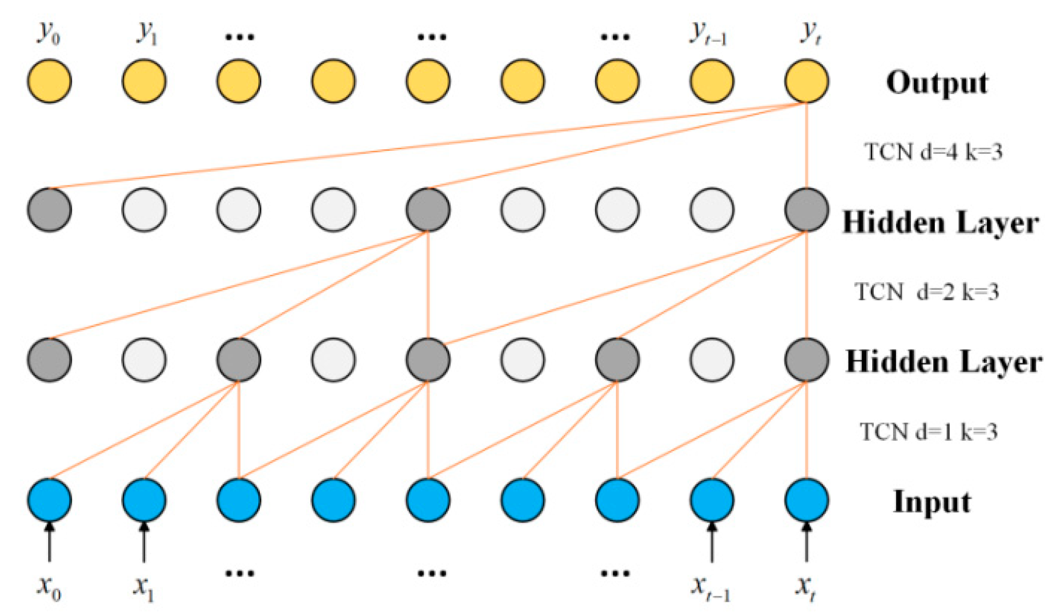
To overcome the limited modeling capacity imposed by the size of the convolution kernel, causal convolution is combined with dilated convolution. Dilated causal convolution expands the receptive field by skipping portions of the input sequence without losing temporal information, as illustrated in Figure 1. The operation of dilated causal convolution $F(s)$ can be formally expressed as follows:

$$F(s)=(x\times df)(s)={\displaystyle \sum _{i=0}^{k-1}f(i)·x_{s-d\times i}}$$

(9)

Here, x is the one-dimensional input sequence, s denotes a sequence element, k is the convolution filter, d is the dilation factor. Increasing d and k expands the receptive field of the convolution, allowing the network to capture more information at each time step.

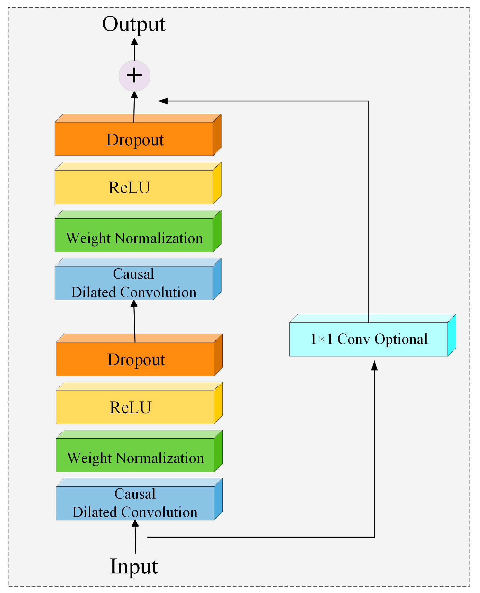
As the length of time-series data increases, deeper networks are required to enhance information processing capabilities. However, increasing network depth can introduce challenges such as network degradation, higher computational cost, gradient vanishing, and gradient explosion [21]. To address these issues, TCN incorporates residual modules. The core idea of the residual module is to use an identity mapping as a shortcut connection, combining inputs and outputs to preserve information while reducing network complexity. This approach improves the stability of TCNs in deeper architectures. A typical TCN residual module consists of a dilated causal convolution layer, WeightNorm normalization, a nonlinearity (ReLU), and a regularized dropout layer, commonly arranged in two stacked layers as illustrated in Figure 2. The module can be formally expressed as:

$$x_{i+1}=h(x_i)+H(x_i,W_i)$$

(10)

where $x_{i+1}$ represents the residual module output, $h(x_i)$ denotes the direct mapping component, $x_i$ signifies the input, $H(x_i,W_i)$ indicates the residual, and $W_i$ represents the weight matrix.

2.1.3. Gated Recurrent Units (GRUs)

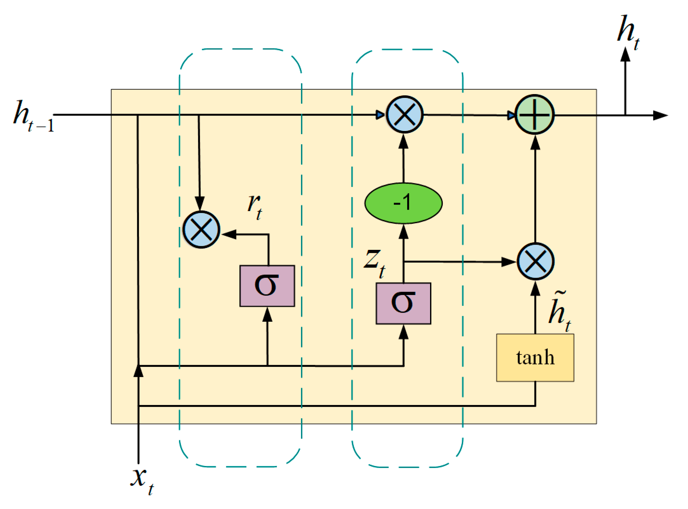
The GRU is a simplified variant of the LSTM network, based on RNNs [22]. It is designed to efficiently capture both long-term and short-term dependencies in sequential data while maintaining a simpler structure and lower computational cost. Unlike LSTM, GRU couples the input and forget gates into a single mechanism, resulting in only two gates: the update gate and the reset gate, as illustrated in Figure 3. The update gate controls how much past information is retained, while the reset gate determines the extent to which previous information is discarded [23]. The operations of a GRU unit can be expressed as follows:

$$z_t=\mathrm{\sigma }(W_z·[h_{t-1},x_t])$$

(11)

$$r_t=\mathrm{\sigma }(W_r·[h_{t-1},x_t])$$

(12)

$${\tilde{h}}_t=\tanh (W_{\tilde{h}}·[r_t*h_{t-1},x_t])$$

(13)

$$h_t=(1-z_t)*h_{t-1}+z*\tilde{h}$$

(14)

where $\mathrm{\sigma }$ represents the sigmoid function, $h_{t-1}$ presents the output of the previous time step, $h_t$ denotes the current output, $x_t$ indicates the current input, $W$ presents the weight of the corresponding formula, and ${\tilde{h}}_t$ signifies the current hidden state information. $z_t$ and $r_t$ represent the update gate and reset gate, respectively. Both control how the cell updates its contents by considering the linear combination of the previous state $h_{t-1}$ and the input $x_t$, $*$ indicates element by element multiplication.

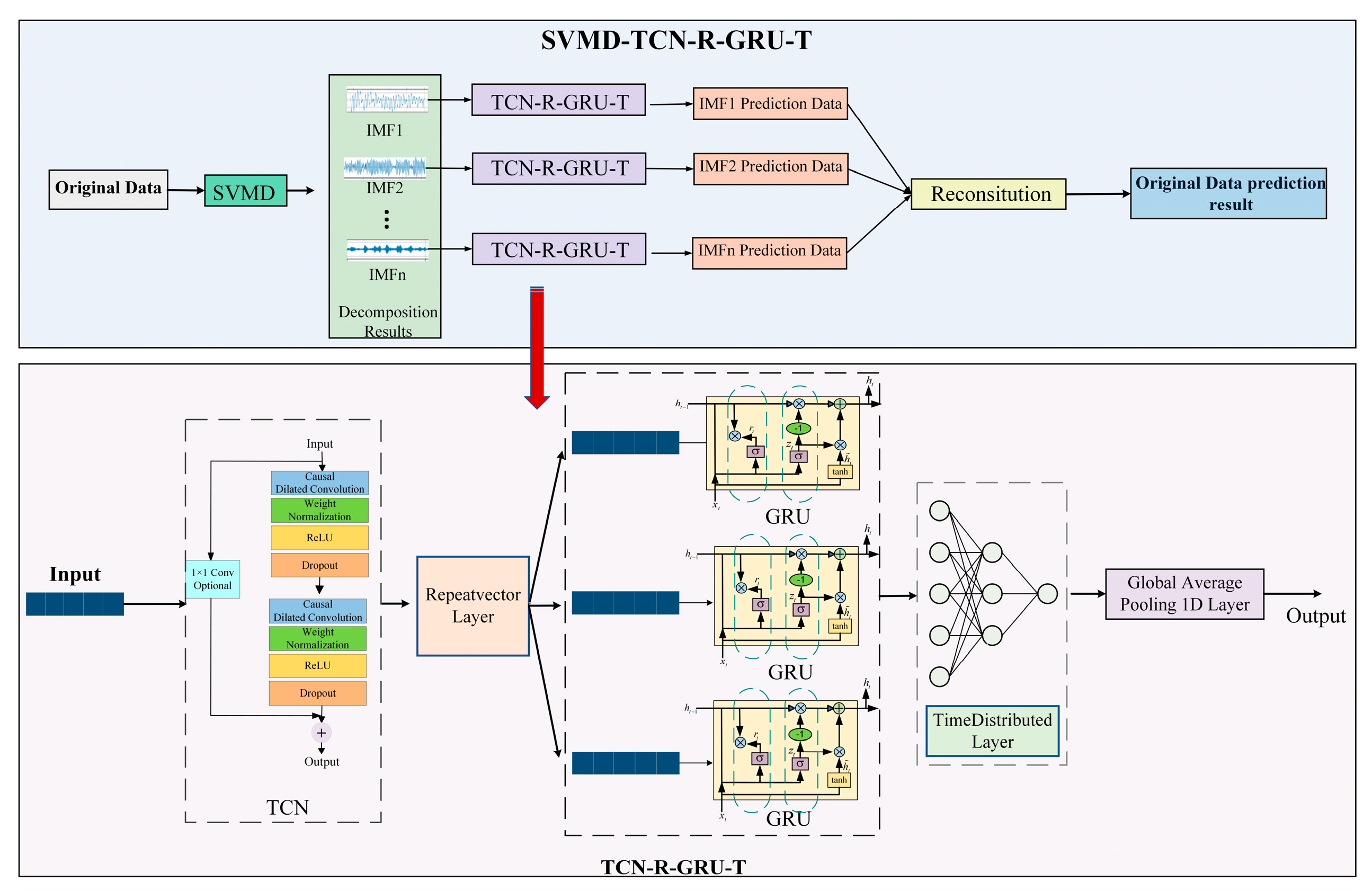
2.1.4. TCN-R-GRU-T Model

To enhance the model’s generalization and multidimensional analysis capabilities, we augmented the traditional TCN-GRU architecture with RepeatVector, TimeDistributed, and GlobalAveragePooling1D layers, forming the improved TCN-R-GRU-T model. First, a RepeatVector layer is added after the TCN. This layer replicates the deep features extracted by the TCN a specified number of times, expanding the input dimensions and introducing additional attribute dimensions, which allows the subsequent GRU layers to analyze multidimensional data more comprehensively. Next, a TimeDistributed layer is added after the GRU, passing each time step of the sequence through a fully connected linear activation layer (Dense). This preserves the temporal independence of each step while sharing weights efficiently, ensuring that the dimensional information introduced by the RepeatVector layer is maintained. Finally, a GlobalAveragePooling1D layer aggregates the expanded dimensions produced by the RepeatVector layer, extracting global features, enhancing prediction accuracy, and further improving the model’s generalization capability.

2.1.5. SVMD-TCN-R-GRU-T Model

The model proposed in this study, termed SVMD-TCN-R-GRU-T (STRGT), combines the advantages of SVMD, GRU, TCN, RepeatVector, TimeDistributed, and GlobalAveragePooling1D layers for predicting agricultural parameters. The overall structure is illustrated in Figure 4. First, the original data are decomposed using SVMD to obtain IMF components with distinct frequency characteristics. Each IMF component is then individually fed into the TCN-R-GRU-T model, enabling the network to more effectively capture the nonlinearity and nonstationarity inherent in the original data. Finally, the predicted values of all IMF components are reconstructed to generate the final prediction of the original data.

This model fully leverages SVMD to overcome modal aliasing caused by an inaccurate number of modes, thereby obtaining an optimal set of IMFs. The TCN captures long-term dependencies and global features within each IMF, while the GRU further models short-term dependencies and dynamic changes. The RepeatVector layer replicates the TCN output along the time dimension, reducing the likelihood that the GRU will miss short-term dependencies and enhancing its ability to capture latent information. The TimeDistributed layer processes each time step through a fully connected layer with shared weights, improving prediction accuracy, stability, and generalization while reducing model complexity. Finally, GlobalAveragePooling1D aggregates the additional dimensions to extract global trends from each IMF, further enhancing forecast stability and generalization. This combination of data decomposition and multi-layered modeling not only improves prediction accuracy but also demonstrates strong capability in handling complex temporal data.

2.2. The FCSDDA

In the previous chapter, we proposed a deep prediction model that generates future prediction signals $F(x)$ for agricultural parameters. Our ultimate goal is to adjust the sampling frequency of sensor nodes by analyzing the variation in these predicted signals $F(x)$, thereby reducing redundant acquisition of low-value data while improving data validity and energy efficiency. To achieve this, it is essential to determine a minimum sampling frequency that ensures the collected data accurately reflects environmental changes without losing its statistical characteristics. Wavelet-based methods are widely recognized as effective for reducing dataset dimensionality while preserving key signal features. Therefore, we apply the discrete wavelet transform (DWT) to the predicted sensor signals $F(x)$ in order to determine the minimum sampling frequency ${\mathit{smp}}_{F\min }$, assuming the original prediction signal $F(x)$ is sampled at the maximum achievable rate ${\mathit{smp}}_F$.

The discrete wavelet transform (DWT) is a multi-resolution analysis method that decomposes the prediction signal F into a detail component D(t) and an approximation component A(t). The length of each decomposed component is ${\displaystyle \frac{1}{2}}$ of the original prediction signal $F(x)$. The approximation coefficients are obtained as the output of the low-pass filter, while the detail coefficients are derived from the output of the high-pass filter. When the prediction signal $F(x)$ is decomposed into n layers, it produces n detail components $D_m(t)$ and one approximation component $A_m(t)$, each with a length of ${\displaystyle \frac{1}{2^m}}$ of the original signal $F(x)$. After decomposition, the approximation component $D_m(t)$ can be discarded, and only the detail component $A_m(t)$ is retained for signal reconstruction, resulting in the reconstructed signal $F{\prime }_m(x)$. This reconstructed signal $F{\prime }_m(x)$ preserves the overall trend and main features of the predicted signal $F(x)$ and can effectively represent the environmental information contained in it. However, as the number of decomposition layers increases, the approximation components capture more information. Consequently, discarding them may cause the reconstructed signal to lose significant portions of the original information $F(x)$.

When the number of decomposition levels reaches a critical value of m + 1, further increasing the levels causes the reconstructed signal $F{\prime }_{m+1}(x)$ to no longer effectively capture the main features of the original prediction signal $F(x)$. At this stage, discarding the approximation components results in the reconstructed signal losing sufficient statistical properties to adequately represent the environmental variations of the original prediction signal $F(x)$. Based on this principle, we define ${\displaystyle \frac{1}{2^m}}$ of the predicted signal sampling frequency ${\mathit{smp}}_{F\min }$ as the minimum sampling frequency ${\mathit{smp}}_{F\min }$. The core idea of this method is that as the number of decomposition layers increases, the signal length decreases proportionally by a factor of ${\displaystyle \frac{1}{2}}$ per layer, while the retained statistical characteristics diminish accordingly. By identifying the critical decomposition level at which the reconstructed signal fails to effectively represent the original signal, we can determine the minimum sampling frequency that preserves the essential characteristics of the signal while maintaining statistical validity.

To quantify the substitution ability of the reconstructed signal for the prediction signal and identify the critical decomposition level, the Spearman rank correlation coefficient is employed as a similarity measure. It is used to calculate the correlation between the predicted signal $F(x)$ and the reconstructed signal at each decomposition layer. When the correlation coefficient between the reconstructed signal and the predicted signal at the mth layer falls below 0.8, it indicates that the reconstructed signal has lost the fundamental characteristics of the predicted signal and can no longer effectively represent it [24]. At this point, ${\displaystyle \frac{1}{2^{m-1}}}{\mathit{smp}}_F$ is defined as the minimum sampling frequency ${\mathit{smp}}_{F\min }$, and m is identified as the critical number of decomposition layers.

After determining the minimum sampling frequency, we propose the FCSDDA to achieve adaptive adjustment of the sensor sampling frequency. The dynamic time warping (DTW), a widely used technique for time-series analysis, measures the degree of change in each segment of the forecast signal relative to its preceding segment. Based on this measurement, the method adaptively selects data points that require sampling. This approach minimizes redundant sampling and reduces energy consumption for low-value data while enhancing data validity.

In this method, we introduce a time step k to replace the sampling frequency. The time step k determines the interval between data collection, and since the sensing interval and sampling frequency are inversely proportional, the following relationship holds: $k_{\min }=1$ denotes the maximum sampling frequency $SM{P}_F$, $k_{\max }=2^{j-1}$ denotes the minimum sampling frequency $sm{p}_{F\min }$, and $smp={\displaystyle \frac{sm{p}_F}{k}}$ defines the conversion relationship between the sampling frequency and k.

From the prediction signal $F(x)=\{x_1,x_2,\dots ,x_n\}$, we extract two subsequences:

$$\begin{array}{c}{d}_{i-1}=\{x_{i-1-lookback},x_{i-lookback},\dots ,x_{i-1}\},\\ d_i=\{x_{i-lookback},x_{i-lookback+1},\dots ,x_i\}.\end{array}$$

(15)

$d_{i-1}$ and $d_i$ represent the previous data subsequence and the current data subsequence, respectively, $lookback<i$, lookback can be set arbitrarily and denotes the amount of backtracking data.

The DTW algorithm is employed to calculate the minimum cumulative distance $D_i$ between two subsequences, which reflects the degree of change in the data points. The core idea of DTW is to construct a cost matrix C using dynamic programming and then compute the minimum cumulative distance. Each element $C_{k,l}$ in matrix C represents the local distance between the kth element of subsequence $d_{i-1}$ and the lth element of subsequence $d_i$.

$$C_{k,l}=|d_{i-1}[k]-d_i[l]|$$

(16)

DTW computes the cumulative cost matrix C* using dynamic programming recursion, which can be expressed by the following recursive formula:

$$C_{k,l}^{*}=C_{k,l}+\min (C_{k-1,l}^{*},C_{k,l-1}^{*},C_{k-1,l-1}^{*})$$

(17)

Finally, $D_i$ is the last element of the cumulative cost matrix C, i.e., $C_{lookback,lookback}$. $D_i$ represents the degree of change of data $x_i$, and $D_1$ corresponds to data $x_{lookback+1}$. Through the DTW calculation, we obtain the distance sequence $D=\{D_1,D_2,\dots ,D_j\}$. However, this sequence $D_i$ only reflects the local variation between the current point $x_i$ and its preceding data. Therefore, we compare the difference in change degree ${|D}_i-D_{i-1}|$ between adjacent data points as the basis for sampling decisions. $∆D_i$ captures the differences in trend changes between data points. A small value indicates that the trends of $x_i$ and $x_{i-1}$ are similar, suggesting that the data value of $x_i$ is low and sampling can be skipped, in which case the step size k is increased by 1. Conversely, a large value indicates a significant change in trend, meaning the data value of $x_i$ is high and sampling is required.

Based on variations in the degree of change in $∆D_i$, we designed a dual-detection mechanism to adaptively adjust the sampling frequency: difference threshold detection and cumulative error detection. When $x_i$ in the predicted signal $F(x)$ satisfies either of these detection mechanisms and the minimum sampling frequency, the sensor collects data for $x_i$ in the future. The sampling interval is set to the current time step k, after which k is reset to 1.

Difference threshold detection: If the absolute value of the difference between the change degree $D_i$ of data $x_i$ in the predicted signal $F(x)$ and the change degree $D_{i-1}$ of its preceding data $x_{i-1}$ exceeds a preset difference threshold ($threshold$), the change in $x_i$ is considered significant compared to the previous data sequence. This point is then identified as high-value data and must be sampled. The corresponding k is recorded as the data collection interval for this instance and is subsequently reset to 1. Otherwise, the point is skipped, and k is incremented by 1. $threshold$ is determined by the average value of $|D_i-D_{i-1}|$ in the change degree sequence D, defined as:

$$\begin{array}{c}threshold={\displaystyle \frac{1}{j-1}}{\displaystyle \sum _{i=1}^{j-1}|D_i-D_{i-1}|},\\ k=\left\{\begin{array}{l}1, if D_i-D_{i-1}|>threshold\\ k+1 , \mathit{otherwise}\end{array}\right..\end{array}$$

(18)

Difference-threshold detection enables dynamic adjustment of the sampling interval when the signal exhibits rapid fluctuations over short periods. However, it is relatively insensitive to slow, long-term changes. Relying solely on difference-threshold detection and the minimum sampling frequency can lead to overly sparse sampling, potentially missing important trend information. To address this limitation, cumulative error detection is introduced to capture gradual, long-term variations, thereby enhancing sensitivity to slowly changing signals and complementing the capabilities of difference-threshold detection.

Cumulative error detection: The cumulative error $aberror$ is defined as the cumulative value $∆D_i$ corresponding to all data points between the most recent actual collection point $x_{i-k}$ and the current point $x_i$. When $aberror$ exceeds the preset threshold $accumulation\_threshold$, the current data point $x_i$ is identified as key trend data and is collected. At this stage, the step length k is recorded as the sampling interval for this collection. The cumulative error $aberror$ and the time step k are then reset. $accumulation\_threshold$ is defined as a multiple of $threshold$, and in this study, it is set to 2. The rationale for this choice will be discussed in the subsequent experiments. The corresponding formula is expressed as follows:

$$\begin{array}{c}aberror=aberror+|D_i-D_{i-1}|,\\ accumulation\_threshold=2\cdot threshold,\\ k=\left\{\begin{array}{l}1, if aberror>accumulation\_threshold\\ k+1, \mathit{otherwise}\end{array}\right..\end{array}$$

(19)

In general, our FCSDDA method is based on the prediction signal $F(x)$. Starting from the lookback + 1th data point at the minimum sampling frequency, it performs change-trend similarity detection on each $x_i$. A dual-detection mechanism then dynamically determines whether to trigger actual sensor sampling at the corresponding moment. The resulting data sampling interval set $K_{\mathit{true}}$ is converted into a data sampling frequency set $SMP$, enabling adaptive sensor sampling. This approach ensures data integrity while reducing redundant sampling, thereby lowering energy consumption and improving data validity. The detailed algorithm flow is presented in Algorithm 1.

Algorithm 1 Frequency conversion sampling method under dual detection analysis

3. Experimental Analysis

3.1. Prediction Model Experimental Analysis

The sensor node dataset used in this study was obtained from the public resources of the Max Planck Institute for Biogeochemistry’s Saaleaue climate station in Jena, Germany. Data were collected from 1 August to 30 August 2024, at 10 min intervals, resulting in a total of 4176 data points. The dataset is divided into training set, validation set, and testing set in a ratio of 7:1:2, and is divided in chronological order. Edge devices (computers) were used to analyze historical temperature data and predict temperature variations for the following day. The predicted values were then compared with actual measurements to evaluate the model’s performance.

3.1.1. Comparing Models and Evaluation Criteria

Traditional CNN-GRU hybrid models generally perform worse than TCN-GRU models in time-series forecasting. In addition, single hybrid models often exhibit weaker predictive performance compared to hybrid models that incorporate data decomposition. To comprehensively evaluate the effectiveness of SVMD in data preprocessing and highlight its advantages over alternative decomposition methods, we included VMD and improved complete ensemble empirical mode decomposition with adaptive noise (ICEEMDAN) as comparative benchmarks in our experiments. Consequently, the experimental results of the SVMD-TCN-R-GRU-T model are compared primarily with CNN-GRU, TCN-GRU, and TCN-R-GRU-T, as well as with decomposition-based hybrid models VMD-TCN-R-GRU-T and ICEEMDAN-TCN-R-GRU-T. To ensure consistency and comparability, all models use six historical time steps to predict the subsequent 10 min interval.

To evaluate and compare the predictive performance of different models, we employed several commonly used error metrics, including mean absolute error (MAE), mean absolute percentage error (MAPE), and root mean square error (RMSE). Lower values of these metrics indicate that a model more accurately fits the data, reflecting stronger predictive capability.

$$MAE={\displaystyle \sum _{i=1}^n|y_i-x_i|}$$

(20)

$$RMSE=\sqrt{{\displaystyle \frac{1}{n}}{\displaystyle \sum _{i=1}^n{(y_i-x_i)}^2}}$$

(21)

$$MAPE={\displaystyle \frac{1}{n}}{\displaystyle \sum _{i=1}^n|\frac{y_i-x_i}{x_i}|}\times 100\%$$

(22)

3.1.2. Decomposition of Temperature Data

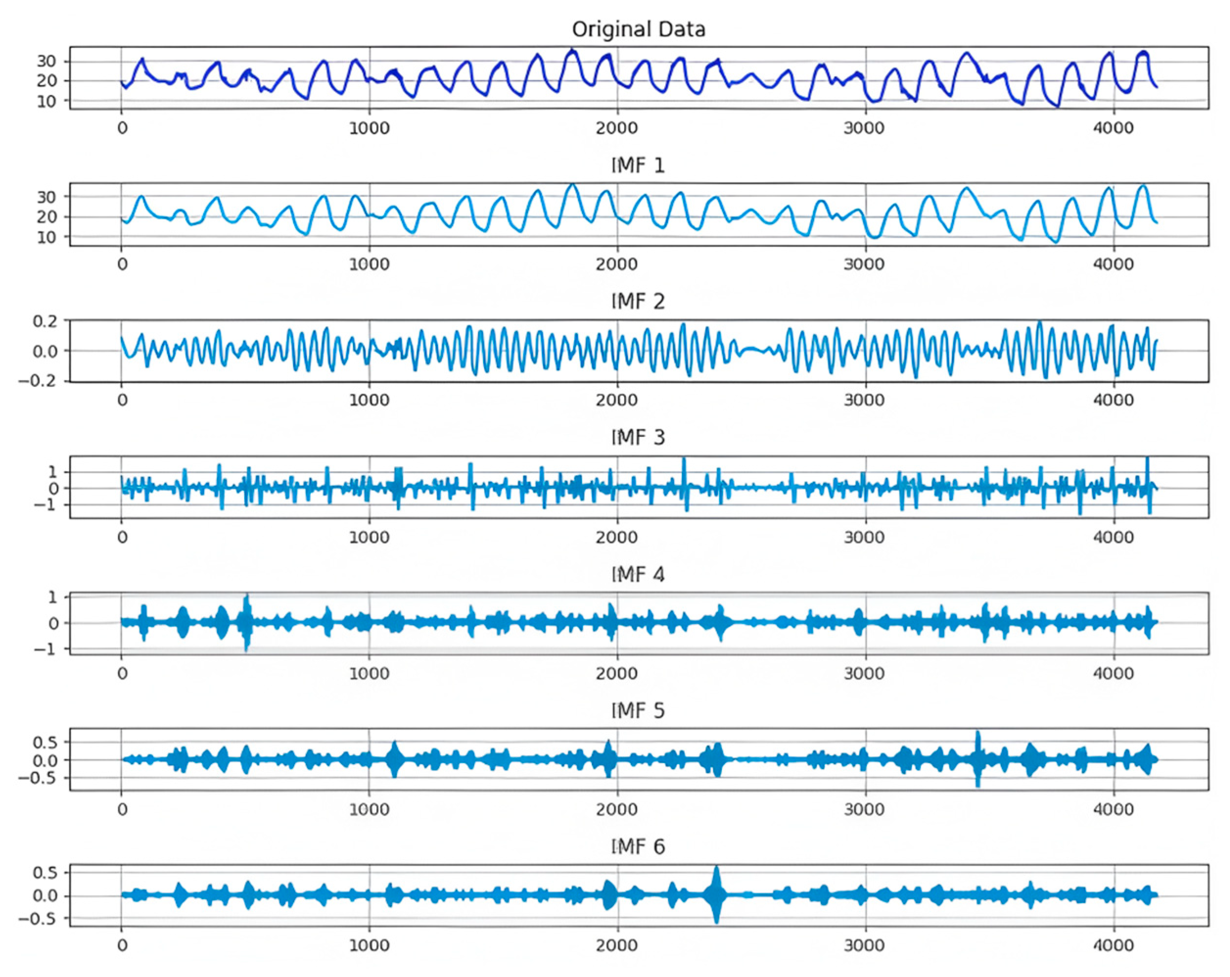
Temperature data exhibit significant nonlinearity and volatility. In this study, SVMD is employed to decompose the data, as it automatically determines the optimal number of modes, avoids modal aliasing, preserves the integrity of the decomposed signal, and enhances prediction accuracy. The decomposition results are presented in Figure 5. The first column shows the original data, followed by the individual IMF components. All IMF components demonstrate regularity, good periodicity, and stability, facilitating feature extraction in subsequent stages of the model.

3.1.3. Model Results and Analysis

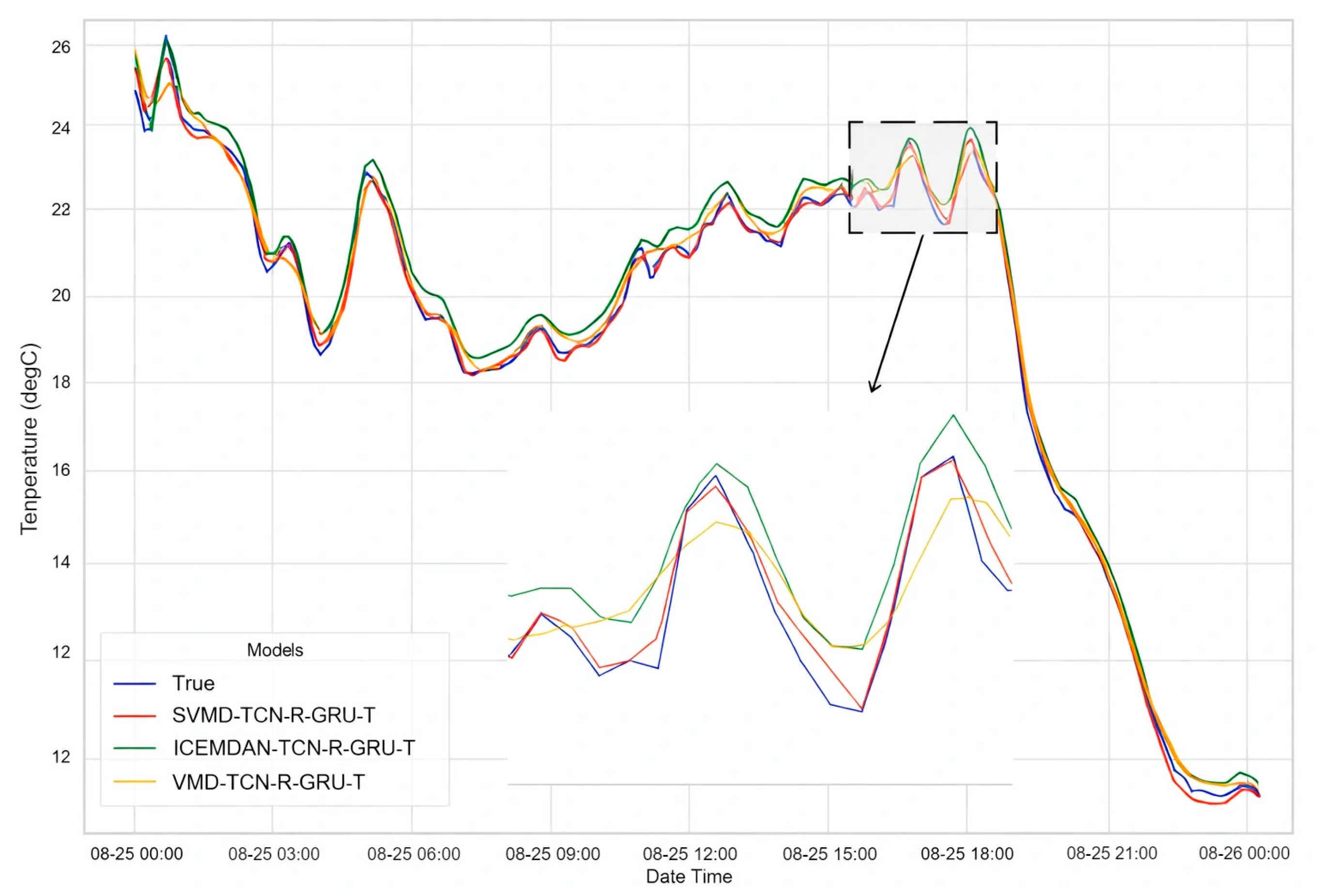
Figure 6 compares the temperature prediction results of the SVMD-TCN-R-GRU-T, VMD-TCN-R-GRU-T, and ICEEMDAN-TCN-R-GRU-T models on 25 August. The SVMD-TCN-R-GRU-T model clearly outperforms the other two models in overall prediction accuracy, particularly around the peaks and troughs of sudden temperature changes, where its predictions align more closely with observed values. This demonstrates that SVMD more effectively captures the dynamic characteristics of temperature data, offering strong predictive accuracy and robustness. In contrast, the VMD and ICEEMDAN decomposition methods are prone to severe mode mixing when processing temperature series, which disrupts the periodicity of the frequency components and increases prediction errors. The SVMD method employed here effectively mitigates mode mixing, accurately extracts the characteristic components of temperature, and improves overall prediction performance.

As shown in

Table 1. Error evaluation results of temperature prediction models.

Model	RMSE	MAE	MAPE
SVMD-TCN-R-GRU-T	0.2087	0.1678	10.04%
ICEEMDAN-TCN-R-GRU-T	0.2767	0.2152	13.35%
VMD-TCN-R-GRU-T	0.2520	0.1952	11.93%
CNN-GRU	0.5864	0.4241	22.51%
TCN-GRU	0.4528	0.3081	19.56%
TCN-R-GRU-T	0.3982	0.2714	14.73%

, among the three decomposition-based hybrid models, SVMD-TCN-R-GRU-T achieves the best performance across all evaluation metrics (RMSE, MAE, and MAPE). Compared with ICEEMDAN-TCN-R-GRU-T, SVMD-TCN-R-GRU-T reduces RMSE, MAE, and MAPE by 24.6%, 22.0%, and 24.8%, respectively. Compared with VMD-TCN-R-GRU-T, the reductions are 17.2%, 14.0%, and 15.8%, respectively. These results highlight the critical role of SVMD in effective data decomposition and its contribution to improving prediction accuracy.

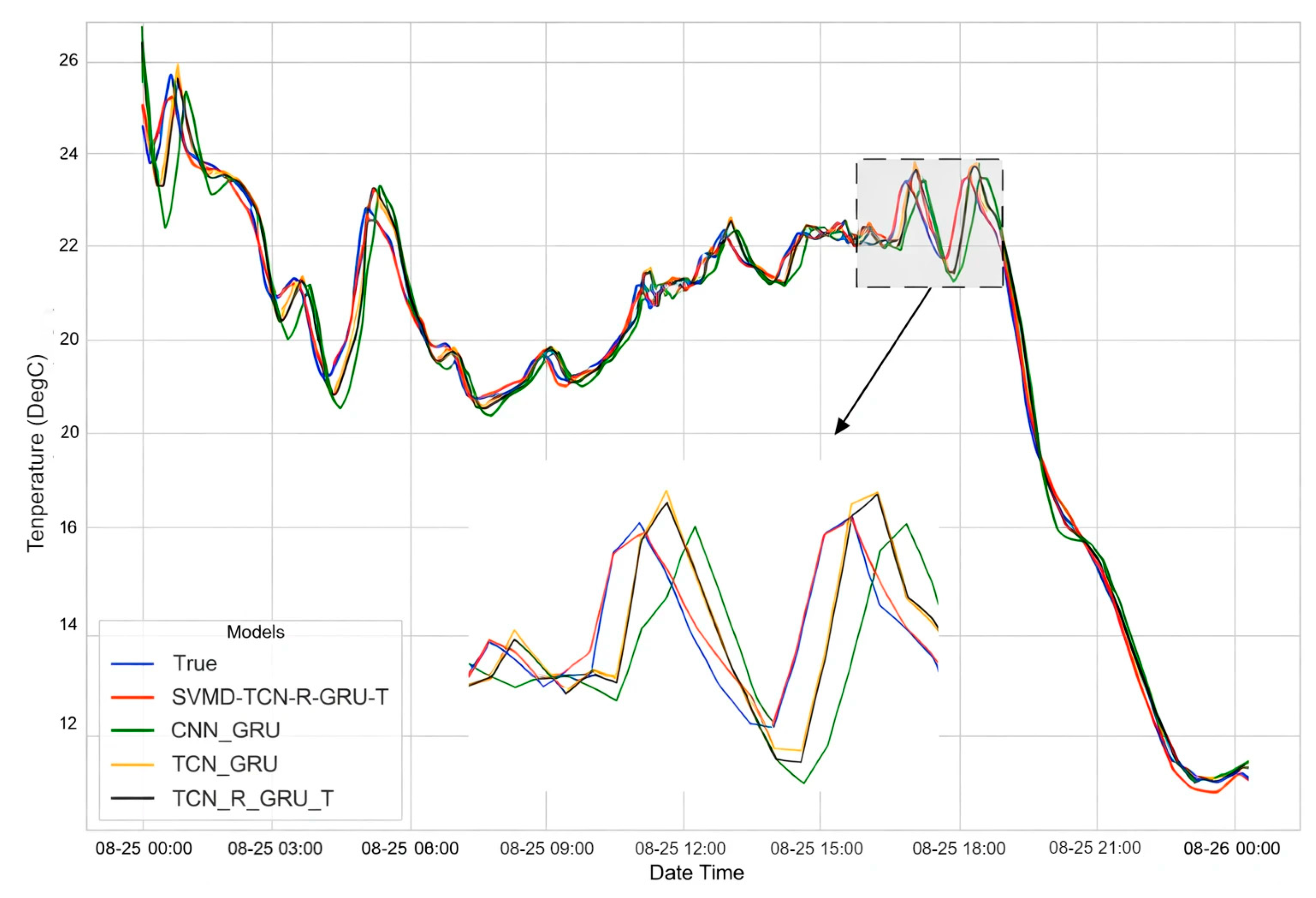
Figure 7 presents the prediction results of SVMD-TCN-R-GRU-T in comparison with three other standalone hybrid models. SVMD-TCN-R-GRU-T clearly outperforms all compared models, delivering the most accurate predictions. Among the standalone models, TCN-R-GRU-T achieves the best performance, with RMSE, MAE, and MAPE values of 0.3982, 0.2714, and 14.73%, respectively. Compared with CNN-GRU, TCN-R-GRU-T reduces RMSE, MAE, and MAPE by 33.1%, 36.0%, and 34.6%, respectively, and compared with TCN-GRU, the reductions are 12.0%, 11.9%, and 24.7%, respectively. These results demonstrate that TCN-R-GRU-T effectively enhances prediction performance, particularly for complex time-series data.

Notably, the CNN-GRU model exhibited the lowest accuracy among all compared models, indicating that TCN is more effective than CNN at capturing the temporal characteristics of temperature time-series data and achieving higher predictive accuracy. Compared with TCN-GRU, the proposed TCN-R-GRU-T model achieves even lower prediction errors. This improvement is attributed to the incorporation of the RepeatVector and TimeDistributed layers, which enhance information transfer and processing of time-series data. Additionally, the GlobalAveragePooling1D layer further strengthens the model’s ability to capture long-term dependencies, enabling it to better handle complex temporal features.

Overall, the SVMD-TCN-R-GRU-T model effectively enhances its ability to handle data complexity and nonlinear features by combining SVMD technology under the experimental conditions of this study. Among all the selected comparison models, the SVMD-TCN-R-GRU-T model exhibits superior temperature prediction accuracy and stability, demonstrating its effectiveness and potential for application in summer temperature agricultural environment prediction tasks.

In addition, Table 1 shows that decomposition-based models exhibit substantially lower prediction errors compared to single models. This indicates that models incorporating data decomposition achieve superior predictive performance relative to standalone models.

3.1.4. Analysis of Prediction Results of Soil Temperature and Moisture

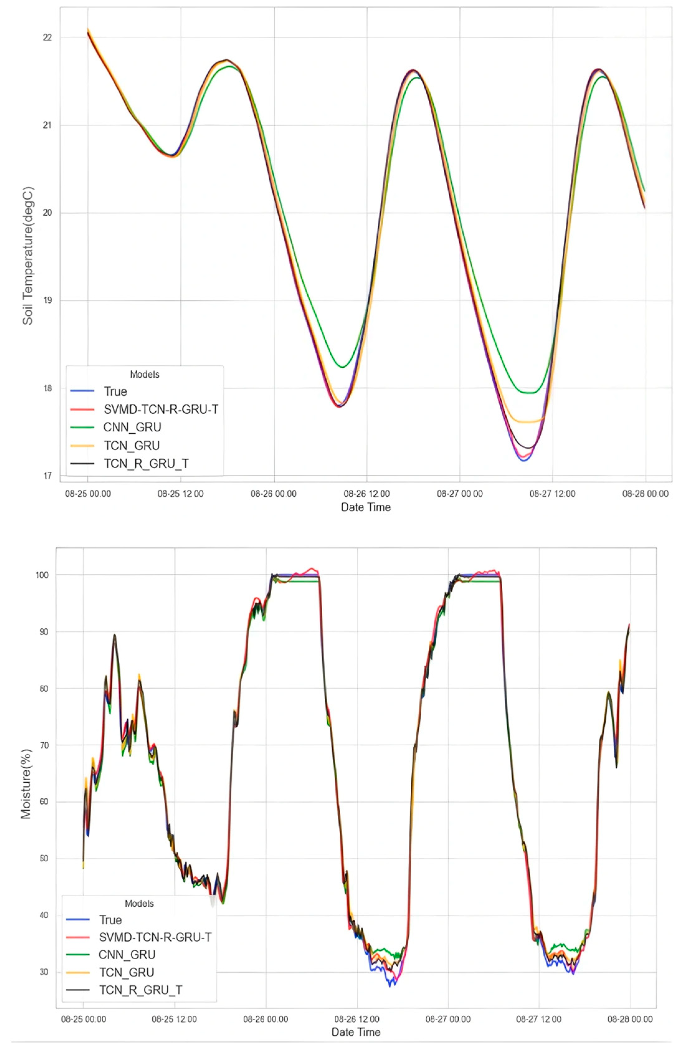
To further validate the effectiveness of our model, we predicted soil temperature and moisture data and presented 3-day prediction results, with the dataset still sourced from publicly available data from the Saaleaue climate station. The models evaluated in this experiment included SVMD-TCN-R-GRU-T, CNN-GRU, TCN-GRU, and TCN-R-GRU-T. The corresponding experimental results are presented in Figure 8.

As shown in Figure 8, all prediction models generally capture the overall trends of soil temperature and moisture. However, deviations are observed when predicting valley values, with the CNN-GRU model exhibiting the lowest accuracy and significant divergence from actual measurements. This highlights the superior ability of TCN to extract deep temporal features compared to CNN. The proposed TCN-R-GRU-T model, which combines TCN and GRU, demonstrates enhanced performance in capturing fluctuations, particularly at soil temperature and moisture valleys. As indicated in

Table 2. Error evaluation results of each model in soil temperature and humidity prediction.

	Model	RMSE	MAE	MAPE
Soil temperature	SVMD-TCN-R-GRU-T	0.0282	0.0200	0.103%
	CNN-GRU	0.2591	0.2066	1.060%
	TCN-GRU	0.1268	0.0996	0.506%
	TCN-R-GRU-T	0.0366	0.0253	0.132%
Moisture	SVMD-TCN-R-GRU-T	0.8770	0.7052	1.374%
	CNN-GRU	1.9999	1.4956	2.988%
	TCN-GRU	1.7932	1.2323	2.491%
	TCN-R-GRU-T	1.4013	0.9852	1.853%

, all three key evaluation metrics show improvements over the TCN-GRU model, illustrating that the incorporation of RepeatVector, TimeDistributed, and GlobalAveragePooling1D layers strengthens the model’s ability to capture long-term dependencies and extract latent information. These structural enhancements allow the model to effectively handle complex temporal patterns, thereby improving prediction accuracy and generalization.

In summary, the SVMD-TCN-R-GRU-T model demonstrates excellent performance in both overall prediction and valley value prediction. Compared with the TCN-R-GRU-T model, it reduces RMSE, MAE, and MAPE for soil temperature predictions by 22.9%, 20.9%, and 22.0%, respectively, and decreases errors for soil moisture predictions by 37.0%, 28.4%, and 25.0%, respectively. These results indicate that data decomposition techniques can effectively enhance the model’s ability to capture complex data structures, further improving prediction accuracy. The SVMD-TCN-R-GRU-T model consistently demonstrates excellent performance in predicting three agricultural environment variables, further highlighting the potential application of agricultural environment prediction tasks related to our test parameters in summer.

3.1.5. Discussion

From Figure 6, Figure 7 and Figure 8 and Table 1 and Table 2, it can be seen that SVMD-TCN-R-GRU-T achieved the best performance in predicting temperature, soil temperature, and humidity. From the overall results, the most significant difference is not reflected in the fitting of the stationary interval, but rather concentrated in the rapid transition period between temperature and soil variables (near peaks and valleys). The reason why SVMD-TCN-R-GRU-T has the best prediction performance mainly comes from two aspects: firstly, SVMD separates the mixed frequency components more clearly in the front end, making it easier for subsequent models to learn stable dynamic patterns, and exhibiting better fit and anti-interference near mutation and extreme values, thereby improving the response ability to key change segments. Secondly, TCN-R-GRU-T improves the aggregation and feature expression capabilities of potential effective information by introducing structures such as RepeatVector, TimeDistributed, and GlobalAveragePooling1D. Compared with CNN-GRU and TCN-GRU, TCN-R-GRU-T is more suitable for modeling complex agricultural time series data. Overall, the combination of SVDD decomposition and time modeling provides more reliable trend estimation support for subsequent FCSDDA. However, it should be pointed out that the current discussion is based on a limited time span sample, and the conclusion should be limited to the tested scenario and seasonal conditions; The robustness against cross seasonal and extreme weather conditions still needs further validation.

3.2. Experimental Analysis of Frequency Conversion Sampling Algorithm

Next, the temperature time-series forecasts for 25 August generated by the SVMD-TCN-R-GRU-T (STRGT) prediction algorithm, deployed on edge devices, were used as input for the FCSDDA algorithm on the same edge devices. The actual data collection rate (maximum rate) was once every 10 min, resulting in a total of 144 data points.

To evaluate the effectiveness of the variable frequency sampling method, we consider the sparsity and distribution of local data sampling, as well as the following metrics: data value density and energy efficiency improvement rate.

Since data collection of agricultural IoT sensor nodes will consume energy, the less the number of data collection is, the more energy efficiency will be improved. Therefore, the less the amount of data collected, the smaller the energy consumption is, the higher the energy efficiency will be improved. Assuming that the energy consumed by each perception is the same, the energy efficiency improvement rate E can be calculated as follows.

$$E=({\displaystyle \frac{N_{total}}{m}}-1)\times 100\%$$

(23)

m is the amount of data collected, and N_total is the total amount of data.

The data value density is calculated as follows:

$${\displaystyle \frac{{\displaystyle \sum _{i=1}^m|D_i-D_{i-1}|}}{m}}$$

(24)

Here $D_i$ is the DTW value corresponding to the actual sampling point obtained by the sampling method.

In Section 2.2, we showed that introducing a cumulative error detection mechanism effectively prevents the loss of trend information caused by signals with similar amplitudes over extended periods. To verify the rationality and effectiveness of the chosen threshold, this section compares the performance of the FCSDDA method under different cumulative thresholds $accumulation\_threshold$, using the configuration $accumulation\_threshold$ = 2 $threshold$ applied in this paper as the baseline for comparative analysis. After preliminary experiments, we selected three additional cumulative error thresholds $accumulation\_threshold$: 1 $threshold$, 1.5 $threshold$, and 2.5 $threshold$, and compared their performance with that of the baseline setting $accumulation\_threshold$ = 2 $threshold$. For clarity, these four FCSDDA methods with different cumulative error thresholds are denoted as 1.0 FCSDDA, 1.5 FCSDDA, 2.0 FCSDDA, and 2.5 FCSDDA, respectively.

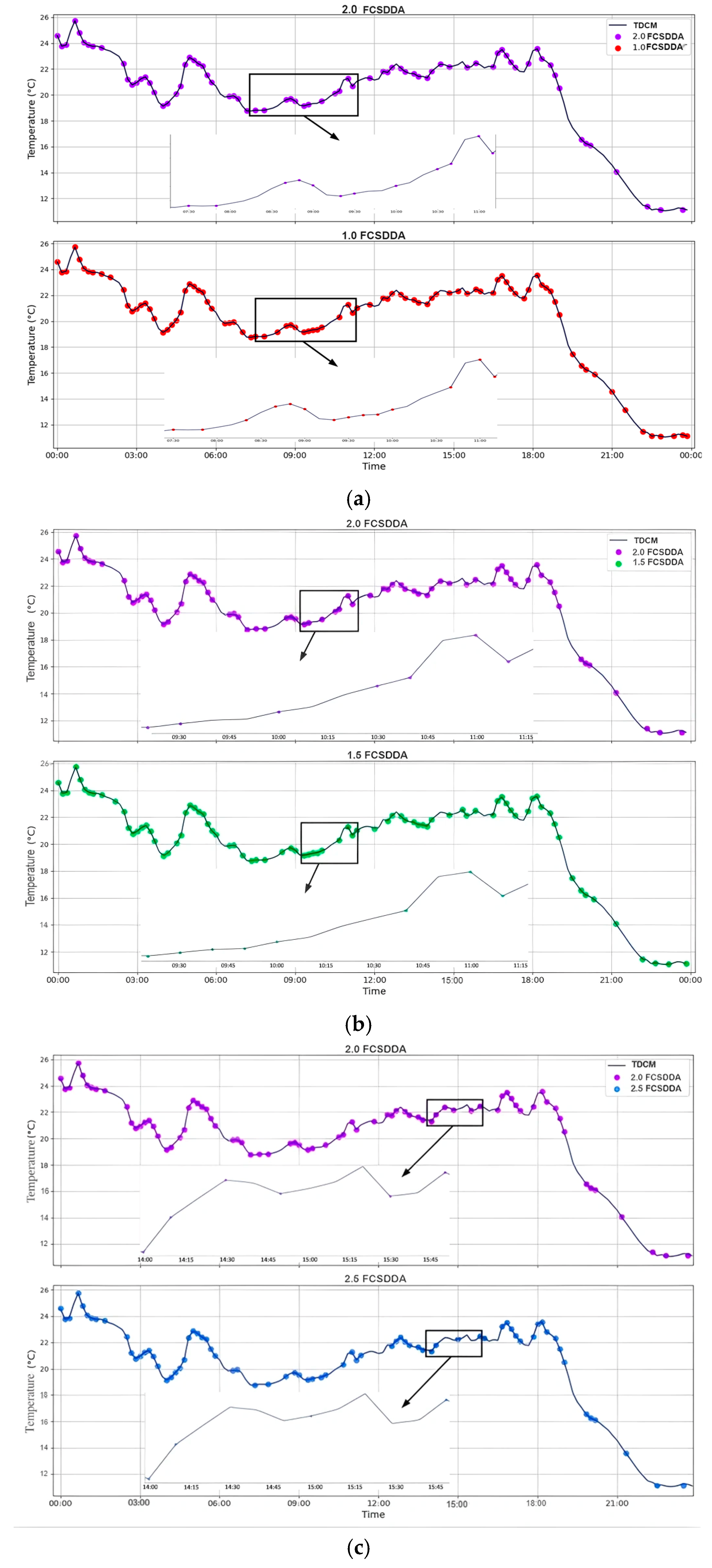
In Figure 9, the black line represents the traditional data collection method (TDCM), which records all data and serves as a reference for observing temperature changes. As shown in Figure 9a, the 1.0 FCSDDA method is highly sensitive to even minor temperature fluctuations, sampling frequently regardless of the magnitude of change. The zoomed-in region highlights two areas of intense fluctuations, with both upward and downward trends, and two areas of gentle upward fluctuations. In regions of intense fluctuation, both 1.0 FCSDDA and 2.0 FCSDDA successfully increase the sampling frequency, reducing sparsity and capturing the full trend. However, in regions of gentle fluctuation, 1.0 FCSDDA still collects 14 data points, leading to overly dense sampling, excessive collection of low-value data, and reduced data validity. In contrast, 2.0 FCSDDA collects only 12 data points while effectively preserving the trend, demonstrating its ability to reduce sampling frequency, lower energy consumption, and improve data validity.

In contrast to the overly dense sampling of the 1.0 FCSDDA method, the 2.5 FCSDDA method, shown in Figure 9c, is excessively sparse, failing to capture key details when changes in the signal are moderate. In the magnified region of Figure 9c, 2.5 FCSDDA collects only four data points, missing most high-value information due to the low sampling frequency. This excessive sparsity renders the data for this period less useful for subsequent analysis. Conversely, 2.0 FCSDDA collects just six data points while successfully capturing the majority of high-value, critical information. The sampled data effectively reflect the overall trend, maximizing the collection of valuable information with minimal redundancy and thereby improving data validity during the acquisition process.

Figure 9b presents the data sampling results for 2.0 FCSDDA and 1.5 FCSDDA. The 1.5 FCSDDA method is more sensitive to data changes, less so than 1.0 FCSDDA, but still captures a substantial amount of detail, albeit with less effectiveness in preserving overall data trends. In the magnified region, an overall upward trend is observed, suggesting that the sampling frequency could be reduced. In this section, 2.0 FCSDDA collected data at a lower and more evenly spaced rate, achieving appropriate sampling sparsity while retaining key information. In contrast, 1.5 FCSDDA sampled more frequently in the first half of the ascending region but used a lower rate in the second half, resulting in unevenly distributed points. Specifically, within the magnified area, 1.5 FCSDDA collected eight data points, whereas 2.0 FCSDDA collected only seven. This illustrates that 2.0 FCSDDA maintains a more balanced sampling distribution, reduces energy consumption, and better preserves data validity.

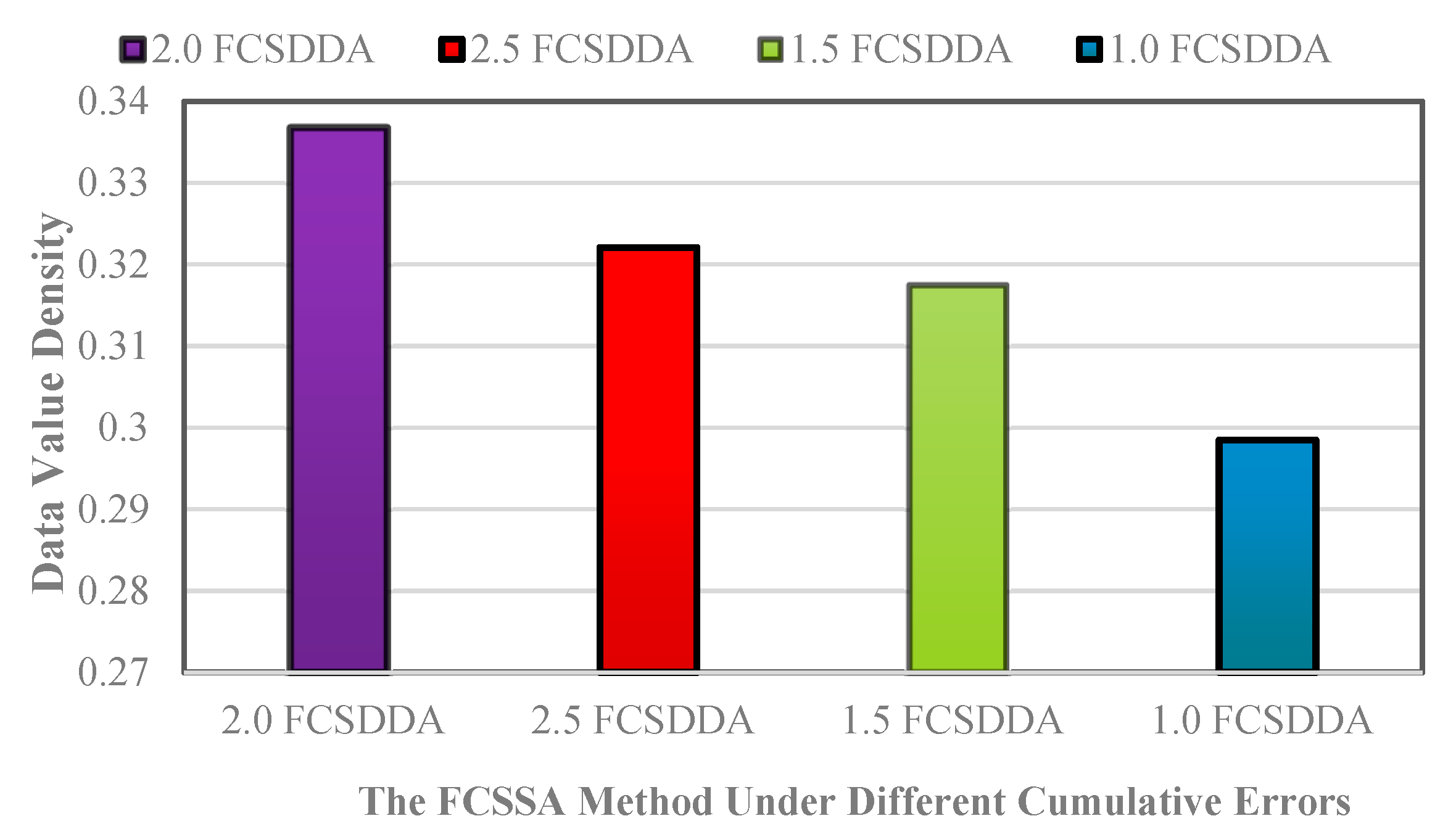
As shown in Figure 10, among the four FCSDDA configurations with cumulative error detection, 2.0 FCSDDA achieves the highest data value density of 0.3368, performing the best overall. This is followed by 2.5 FCSDDA, with a data value density of 0.3221, while 1.0 FCSDDA performs the worst, with a data value density below 0.3. These results indicate that the cumulative error threshold of 2.5 FCSDDA is too high, leading to a low sampling frequency for overall dynamic changes. As a result, it fails to capture sufficient key information and risks omitting high-value and important data. Conversely, the $accumulation\_threshold$ thresholds of 1.5 FCSDDA and 1.0 FCSDDA are too low, making the method overly sensitive to minor fluctuations. Although such settings capture more detailed changes, they also introduce a large volume of low-value data. The configuration $accumulation\_threshold$ = 2 $threshold$ used in 2.0 FCSDDA strikes an effective balance: it successfully detects long-term variations in the temperature prediction signal. When the signal fluctuates significantly, the sampling frequency increases appropriately to capture high-value, critical data. When the signal remains stable, the sampling frequency decreases to avoid redundant collection of low-value data. This adaptive adjustment effectively enhances data validity.

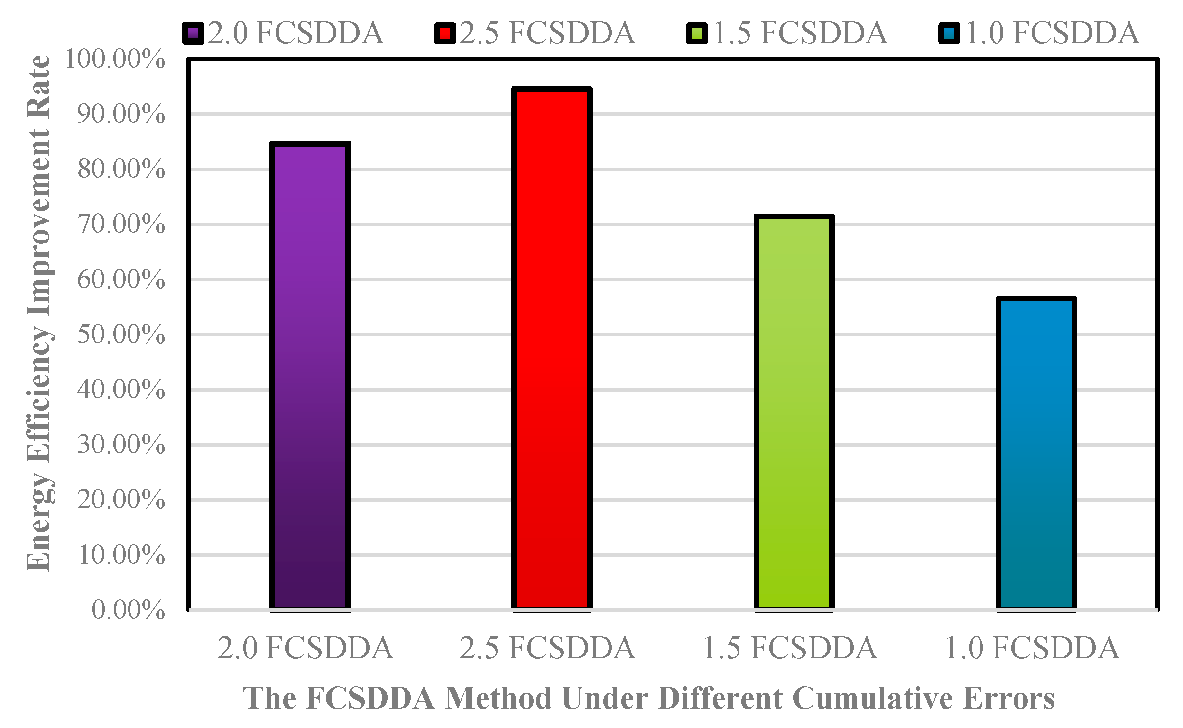
Figure 11 illustrates the energy efficiency improvements rate of the FCSDDA method compared to TDCMs under four cumulative error thresholds. The 2.5 FCSDDA achieves the highest energy efficiency improvement rate at 94.59%, with a data collection rate of 51.38%. The 2.0 FCSDDA follows closely, achieving an 84.61% improvement and a data collection rate of 54.16%. In contrast, the 1.5 FCSDDA and 1.0 FCSDDA achieve lower energy efficiency improvements rate of 71.42% and 56.52%, with corresponding data collection rates of 58.33% and 63.88%, respectively. However, simply maximizing energy savings or minimizing sampling frequency is not the fundamental goal of variable frequency sampling. The objective is to reduce sampling while ensuring the collection of high-value, critical data, thereby improving both energy efficiency and data validity. As shown in Figure 9 and Figure 10, although 2.5 FCSDDA achieves the highest energy efficiency improvements rate, its excessively sparse sampling leads to the loss of critical information, reducing data value density and the reliability of subsequent analyses. Conversely, 1.5 FCSDDA and 1.0 FCSDDA are overly sensitive to small fluctuations, collecting large amounts of low-value data. While these models preserve data variability, they do not effectively enhance energy efficiency or data value density. A comprehensive analysis indicates that 2.0 FCSDDA strikes the optimal balance between energy efficiency improvements rate and data value density, with a cumulative error threshold of 2 $threshold$ being the most appropriate setting.

As discussed in Section 2, the effectiveness of prediction-based variable frequency sensing methods is closely tied to prediction accuracy. To examine the impact of prediction accuracy on the performance of the proposed FCSDDA method, we conducted experiments using the CNN-GRU, TCN-GRU, and STRGT prediction models to forecast the temperature signal for August 25. The resulting predictions were then used as input for the FCSDDA method. Accordingly, the FCSDDA variants based on these models are referred to as CNN_GRU FCSDDA, TCN_GRU FCSDDA, and STRGT FCSDDA, respectively.

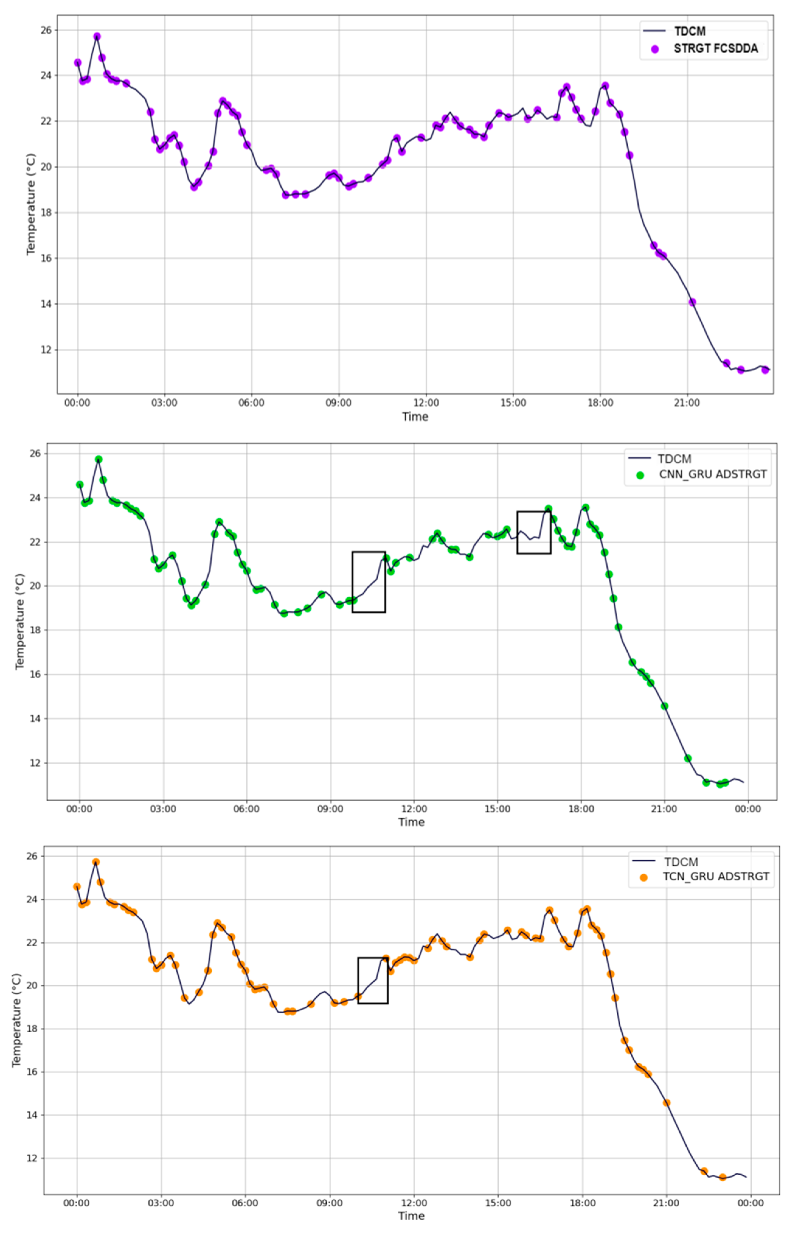
Figure 12 presents the data sampling results for CNN_GRU FCSDDA, TCN_GRU FCSDDA, and STRGT FCSDDA. During the period from 9:00 to 12:00 (highlighted in the left black box), the sampling frequency of CNN_GRU FCSDDA and TCN_GRU FCSDDA are too low, resulting in excessive sparsity and failure to capture the basic fluctuation trends of the actual temperature curve. Notably, the CNN_GRU FCSDDA model, which exhibits the poorest prediction accuracy, completely fails to capture temperature changes between 15:50 and 16:50 (right black box), an interval of intense variation, leading to total data loss. This failure stems from the low-precision predictions of CNN-GRU and TCN-GRU, which deviate substantially from the true temperature values. Consequently, FCSDDA misinterprets this interval as stable, applying an unreasonably sparse sampling strategy and severely compromising data validity. In contrast, STRGT FCSDDA achieves the highest accuracy, as its predictions closely match the actual data. This allows FCSDDA to correctly assess the degree of data variability, adopt an appropriate sampling frequency, retain high-value key data, and produce the most reliable sampling results.

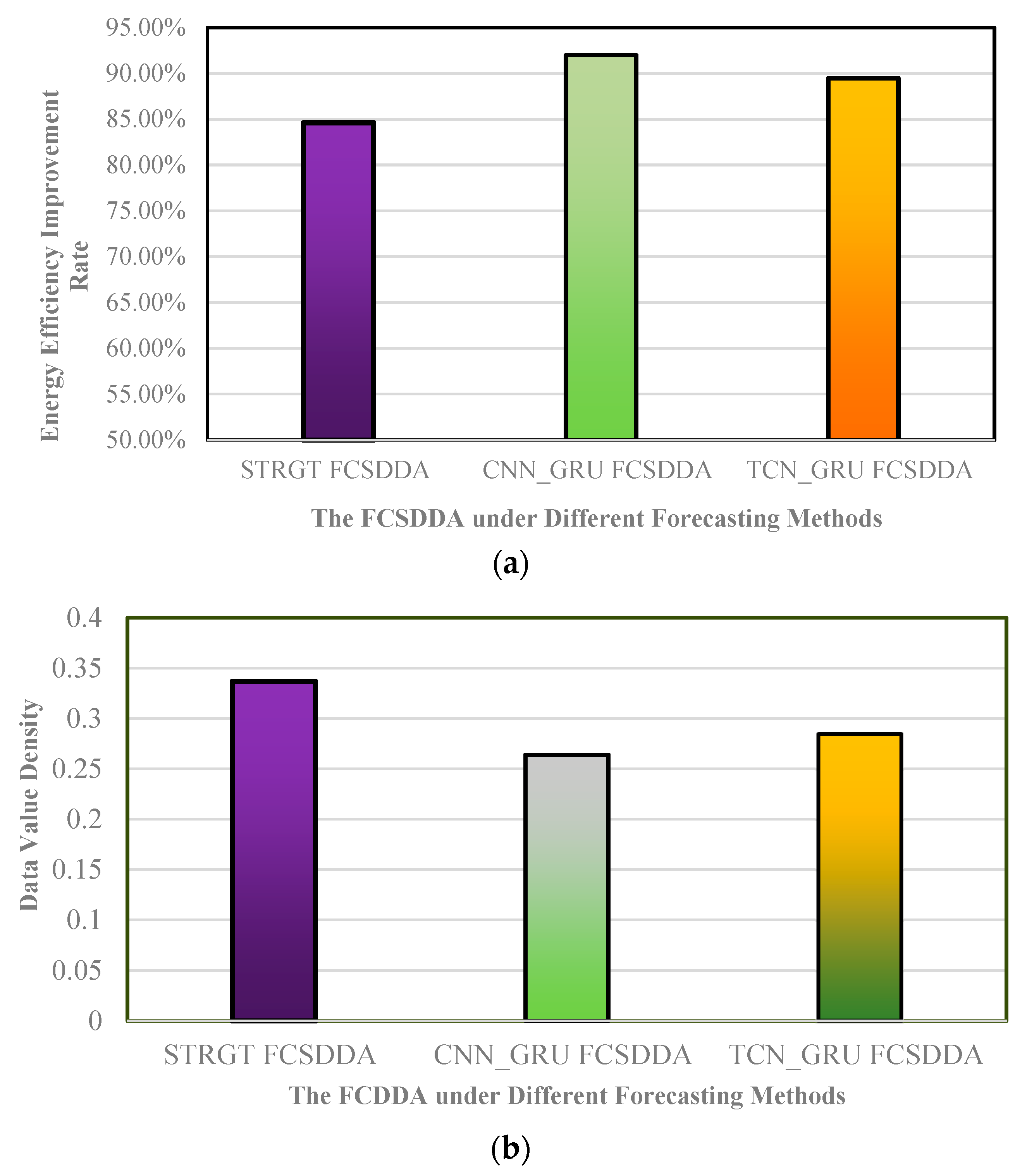
Figure 13 presents a comprehensive evaluation of two key metrics, energy efficiency improvement rate and data value density, highlighting the impact of prediction accuracy on FCSDDA performance. In Figure 13a, CNN_GRU FCSDDA achieves the highest energy efficiency improvement rate at 92%, with a sampling frequency of 52.08%, followed by TCN_GRU FCSDDA at 89.47% with a 52.77% sampling frequency. STRGT FCSDDA shows slightly lower energy efficiency improvement rate but excels in data value density (Figure 13b), achieving 0.3368 compared to 0.2641 for CNN_GRU FCSDDA (78.41% of STRGT FCSDDA) and 0.2847 for TCN_GRU FCSDDA (84.53% of STRGT FCSDDA). Although CNN_GRU FCSDDA and TCN_GRU FCSDDA achieve marginally higher energy efficiency (about 7–8 percentage points), their data value density drops by 15.6–21.5%. This occurs because low-precision prediction models misjudge periods of rapid change, resulting in severe undersampling during key intervals (e.g., 9:00–12:00 and 15:50–16:50) and loss of high-value data, while maintaining unnecessarily high sampling rates during stable periods. In contrast, STRGT FCSDDA accurately identifies high- and low-value regions, maintains appropriate sampling during critical periods, and avoids resource waste in low-value intervals, achieving superior data validity (0.3368) while sustaining competitive energy efficiency. This demonstrates that high-accuracy prediction models are essential for balancing energy savings and data value in adaptive sampling.

The experimental results above demonstrate a strong correlation between prediction accuracy and the performance of prediction-based variable frequency sensing methods. To achieve optimal data collection outcomes, it is crucial to prioritize high-accuracy prediction models when implementing such algorithms.

4. Conclusions

To address the challenges of low data validity and energy efficiency in agricultural IoT data collection, this paper proposes a novel prediction-based variable frequency sensing method that dynamically adjusts sensor node sampling frequency. First, we developed the STRGT deep prediction model, using SVMD to decompose the data and better capture the nonlinearity and nonstationarity of the original signals. We further enhanced the TCN-GRU architecture by incorporating RepeatVector, TimeDistributed, and GlobalAveragePooling1D layers, improving both the model’s generalization and multidimensional analysis capabilities. The simulation experiment results show that STRGT significantly outperforms traditional models in RMSE, MAE, and MAPE when predicting key agricultural environmental parameters, such as temperature and soil moisture, providing a reliable foundation for subsequent variable frequency sampling.

Secondly, we developed the FCSDDA, which employs wavelet transform to determine the minimum sampling rate and uses DTW to evaluate the degree of signal change. The method incorporates a dual detection mechanism, combining differential error and cumulative error, to accurately identify data trends and dynamically adjust the sampling rate. The simulation experiment results show that, with optimal parameter settings, FCSDDA achieves an effective balance between energy efficiency and data value density. Furthermore, our analysis confirms a positive correlation between prediction accuracy and FCSDDA performance: while FCSDDA using the high-accuracy SVMD-TCN-R-GRU-T model shows a 6–7% lower energy efficiency compared to low-precision prediction models, it increases data value density by over 15%, resulting in superior overall sampling effectiveness.

A potential research direction for future studies is to introduce more agricultural parameters and data from seasons outside of summer to validate our method and demonstrate its generality. Another important direction is to use real-world sensor network environments and IoT hardware to validate the proposed method.

References

1. Li, X.; Ma, Z.; Zheng, J.; Liu, Y.; Zhu, L.; Zhou, N. An effective edge-assisted data collection approach for critical events in the SDWSN-based agricultural internet of things. Electronics 2020, 9, 907. [Google Scholar] [CrossRef]
2. Ahmed, N.; De, D.; Hussain, I. Internet of Things (IoT) for smart precision agriculture and farming in rural areas. IEEE Internet Things J. 2018, 5, 4890–4899. [Google Scholar] [CrossRef]
3. Huo, D.; Malik, A.W.; Ravana, S.D.; Rahman, A.U.; Ahmedy, I. Mapping smart farming: Addressing agricultural challenges in data-driven era. Renew. Sustain. Energy Rev. 2024, 189, 113858. [Google Scholar] [CrossRef]
4. Et-Taibi, B.; Abid, M.R.; Boufounas, E.; Morchid, A.; Bourhnane, S.; Hamed, T.A.; Benhaddou, D. Enhancing water management in smart agriculture: A cloud and IoT-Based smart irrigation system. Results Eng. 2024, 22, 102283. [Google Scholar] [CrossRef]
5. Ruipeng, T.; Jianbu, Y.; Jianrui, T.; Aridas, N.K.; Talip, M.S.A. Design of agricultural wireless sensor network node optimization method based on improved data fusion algorithm. PLoS ONE 2024, 19, e308845. [Google Scholar] [CrossRef] [PubMed]
6. Čulić Gambiroža, J.; Mastelić, T.; Nižetić Kosović, I.; Čagalj, M. Dynamic monitoring frequency for energy-efficient data collection in Internet of Things. J. Comput. Sci. 2022, 64, 101842. [Google Scholar] [CrossRef]
7. Abdelmoneim, A.A.; Kimaita, H.N.; Al Kalaany, C.M.; Derardja, B.; Dragonetti, G.; Khadra, R. IoT sensing for advanced irrigation management: A systematic review of trends, challenges, and future prospects. Sensors 2025, 25, 2291. [Google Scholar] [CrossRef]
8. Gupta, M.; Shum, L.V.; Bodanese, E.; Hailes, S. Design and evaluation of an adaptive sampling strategy for a wireless air pollution sensor network. In Proceedings of the 2011 IEEE 36th Conference on Local Computer Networks, Bonn, Germany, 4–7 October 2011; IEEE: New York, NY, USA, 2011; pp. 1003–1010. [Google Scholar]
9. Ye, Q.; Szeto, W.Y.; Wong, S.C. Short-term traffic speed forecasting based on data recorded at irregular intervals. IEEE Trans. Intell. Transp. Syst. 2012, 13, 1727–1737. [Google Scholar] [CrossRef]
10. Werner-Allen, G.; Johnson, J.; Ruiz, M.; Lees, J.; Welsh, M. Monitoring volcanic eruptions with a wireless sensor network. In Proceedings of the Second European Workshop on Wireless Sensor Networks, Istanbul, Turkey, 2 February 2005; IEEE: New York, NY, USA, 2005; pp. 108–120. [Google Scholar]
11. Monteiro, L.C.; Delicato, F.C.; Pirmez, L.; Pires, P.F.; Miceli, C. Dpcas: Data prediction with cubic adaptive sampling for wireless sensor networks. In Proceedings of the Green, Pervasive, and Cloud Computing: 12th International Conference, GPC 2017, Cetara, Italy, 11–14 May 2017; pp. 353–368. [Google Scholar]
12. Cecchinel, C.; Fouquet, F.; Mosser, S.; Collet, P. Leveraging live machine learning and deep sleep to support a self-adaptive efficient configuration of battery powered sensors. Future Gener. Comput. Syst. 2019, 92, 225–240. [Google Scholar] [CrossRef]
13. Hussein, A.M.; Idrees, A.K.; Couturier, R. Distributed energy-efficient data reduction approach based on prediction and compression to reduce data transmission in IoT networks. Int. J. Commun. Syst. 2022, 35, e5282. [Google Scholar] [CrossRef]
14. Fathalla, A.; Li, K.; Salah, A.; Mohamed, M.F. An LSTM-based distributed scheme for data transmission reduction of IoT systems. Neurocomputing 2022, 485, 166–180. [Google Scholar] [CrossRef]
15. Jarwan, A.; Sabbah, A.; Ibnkahla, M. Data transmission reduction schemes in WSNs for efficient IoT systems. IEEE J. Sel. Areas Commun. 2019, 37, 1307–1324. [Google Scholar] [CrossRef]
16. Khan, M.N.; Lee, S.; Shah, M. Adaptive Scheduling in Cognitive IoT Sensors for Optimizing Network Performance Using Reinforcement Learning. Appl. Sci. 2025, 15, 5573. [Google Scholar] [CrossRef]
17. Nazari, M.; Sakhaei, S.M. Successive variational mode decomposition. Signal Process. 2020, 174, 107610. [Google Scholar] [CrossRef]
18. Parri, S.; Teeparthi, K. SVMD-TF-QS: An efficient and novel hybrid methodology for the wind speed prediction. Expert Syst. Appl. 2024, 249, 123516. [Google Scholar] [CrossRef]
19. Zeng, L.; Ning, C.; Fang, Y.; Li, C.; Ji, Y.; Li, H.; Shao, W. Research on Non-Stationary Tidal Level Prediction Based on SVMD and BiLSTM. J. Mar. Sci. Eng. 2025, 13, 1860. [Google Scholar] [CrossRef]
20. Bai, S.; Kolter, J.Z.; Koltun, V. An empirical evaluation of generic convolutional and recurrent networks for sequence modeling. arXiv 2018, arXiv:1803.01271. [Google Scholar] [CrossRef]
21. Li, W.; Wei, Y.; An, D.; Jiao, Y.; Wei, Q. LSTM-TCN: Dissolved oxygen prediction in aquaculture, based on combined model of long short-term memory network and temporal convolutional network. Environ. Sci. Pollut. R. 2022, 29, 39545–39556. [Google Scholar] [CrossRef]
22. Wang, J.; Wang, P.; Tian, H.; Tansey, K.; Liu, J.; Quan, W. A deep learning framework combining CNN and GRU for improving wheat yield estimates using time series remotely sensed multi-variables. Comput. Electron. Agric. 2023, 206, 107705. [Google Scholar] [CrossRef]
23. Cho, K. On the properties of neural machine translation: Encoder-decoder approaches. arXiv 2014, arXiv:1409.1259. [Google Scholar] [CrossRef]
24. Liao, Q.; Xie, L.; Han, J.; Zhang, X. Research on the evolution of global rare earth metals trade network pattern and the propagation of supply crisis. China Min. Mag. 2025, 34, 26–37. [Google Scholar]
Figure 1. Expanded causal convolution.
Electronics 15 00375 g001
Figure 2. Residual structure of TCN.
Electronics 15 00375 g002
Figure 3. The GRU unit.
Electronics 15 00375 g003
Figure 4. SVMD-TCN-R-GRU-T and TCN-R-GRU-T.
Electronics 15 00375 g004
Figure 5. SVMD results.
Electronics 15 00375 g005
Figure 6. Comparison with Model Predictions Based on Data Decomposition.
Electronics 15 00375 g006
Figure 7. Comparison with Prediction Results from Standalone Prediction Models.
Electronics 15 00375 g007
Figure 8. Comparison of Prediction Results for Soil Temperature (Top) and Moisture (Bottom) Among Different Models.
Electronics 15 00375 g008
Figure 9. It shows the overall and local data sampling results of FCSDDA under different cumulative error thresholds (a) Comparison of data collection results between 1.0 FCSDDA and 2.0 FCSDDA (b) Comparison of data sampling results between 1.5 FCSDDA and 2.0 FCSDDA (c) between 2.5 FCSDDA and 2.0 Comparison of FCSDDA data sampling results.
Electronics 15 00375 g009
Figure 10. Data Value Density of FCSDDA at Different Cumulative Error Thresholds.
Electronics 15 00375 g010
Figure 11. Energy Efficiency Improvement Rate of FCSDDA at Different Cumulative Error Thresholds.
Electronics 15 00375 g011
Figure 12. FCSDDA Data Sampling Results Under Different Prediction Models.
Electronics 15 00375 g012
Figure 13. Energy Efficiency Improvement Rate and Data Value Density of FCSDDA Under Different Prediction Models (a) Energy Efficiency Improvement Rate of FCSDDA Under Different Prediction Models (b) Data Value Density of FCSDDA Under Different Prediction Models.
Electronics 15 00375 g013