Lightweight Multi-Task CNN for Simultaneous IGBT Switch Aging Diagnosis Using CWT-Based RGB Images

Abstract

The per-switch condition monitoring of insulated-gate bipolar transistors (IGBTs) underpins condition-based inverter maintenance, yet existing approaches collapse the six-switch state space into one system-level label, leaving individual devices unresolved. This paper presents a Continuous Wavelet Transform Multi-Task Network (CWT-MTNet), a lightweight convolutional network that predicts the four-class aging state (Healthy, Mild, Moderate, or Severe) of all six switches from one CWT-based RGB image whose channels carry the scalograms of three symmetrical-component deviation signals. Five Depthwise Separable Convolution (DS-Conv) blocks and six classification heads give 172 K parameters in a 0.7 MB footprint—a 21-fold reduction over MobileNet-v2—within the on-chip memory of an embedded inverter controller, a footprint comparison rather than a demonstrated implementation. Trained from scratch on 15,625 samples spanning all $5^6$ state combinations, it attains 98.15 ± 0.33% accuracy and 95.81 ± 0.82% Mild recall over five seeds: within 0.84 percentage points of MobileNet-v2 in accuracy, statistically indistinguishable in Mild recall, at one twenty-first of the parameters. Scratch training outperforms ImageNet pretraining, indicating a domain mismatch with CWT scalograms. Multi-task gradient conflict costs ResNet-18 42.1 points of Mild recall under six-head operation; DS-Conv architectures change by at most 3.3. Grad-CAM attributes this to distributed time–frequency attention; Mild-to-Healthy confusion is the dominant safety risk. A representation ablation shows the CWT recovers 2.4 of the 4.0 points lost by discarding phase and makes per-switch accuracy twelve times more uniform, without being necessary here. Independent sensor noise at 0.5% of the phase RMS exceeds the aging signature sixfold and defeats every encoding examined, so the pipeline requires coherent averaging at the acquisition front end.

1. Introduction

A three-phase voltage-source inverter (VSI) carries six insulated-gate bipolar transistors (IGBTs), and no two of them age at the same rate: junction temperature, switching duty, and thermal-interface quality all differ from device to device. Maintenance, however, is performed one device at a time. A diagnostic system that reports only whether the inverter as a whole has degraded therefore does not address the decision the operator actually faces: which module to replace, and when. Closing that gap means resolving the condition of all six switches independently, and doing so from measurements the drive already takes.

The stakes are set by how often these devices fail. Field surveys attribute roughly 31–34% of power-stage outages to IGBT degradation [1,2], and the cost of an unplanned outage scales with the application—lost generation in multi-megawatt wind and photovoltaic plants, the loss of propulsion in safety-critical aerospace platforms [1,3]. Degradation is nevertheless gradual rather than abrupt. Repeated thermal cycling drives bond-wire lift-off and solder-joint cracking, carrying a device through distinguishable stages—Healthy → Mild → Moderate → Severe—before terminal failure. The evolution of on-state resistance $R_{\mathrm{ON}}$ with aging depends on the measurement convention. Under actual high-temperature inverter operation, an elevated junction temperature dominates the resistance characteristic and causes $R_{\mathrm{ON}}$ to increase with degradation. Under standardized measurement at a 25 °C case temperature, however, accelerated-ageing hardware studies report the opposite: Dimech and Dawson measured a $22.3\%$ average decrease in effective on-state resistance across eight devices after three ageing iterations, alongside X-ray evidence of progressive die-attach voiding [4,5]. This work adopts the cold-measurement convention: $R_{\mathrm{ON}}$ decreases monotonically from 0.007 $\mathrm{\Omega }$ at the near-ideal Master reference to 0.005 $\mathrm{\Omega }$ at the Severe stage, providing a consistent aging proxy independent of operating-point temperature. Crucially, each stage introduces measurable anomalies in the inverter’s output voltage waveforms well before hard failure, opening a window for condition-based maintenance that can prevent unplanned outages and reduce the cost of reactive repairs.

Two families of methods have been developed to read those anomalies. Physics-based monitoring measures aging-sensitive device parameters directly—the collector–emitter saturation voltage $V_{\mathrm{CE},\mathrm{sat}}$, thermal resistance $R_{\mathrm{th}}$, or gate-threshold voltage—as proxies for $R_{\mathrm{ON}}$ [1]. It is accurate under laboratory control, but requires isolated measurement hardware, is confounded by operating-point drift, and adds failure points of its own once embedded in a field system. Signal-processing methods avoid the added instrumentation entirely by deriving degradation indicators from voltages the controller already samples.

The authors’ earlier work followed the latter route twice. In [5], Fortescue symmetrical-component deviations ($\Delta v_0$, $\Delta v_1$, $\Delta v_2$) were reduced to scalar features and fed to a shallow artificial neural network, yielding 94.49% Risk Level accuracy and $R^2=0.8718$ for Combined Aging Index (CAI) regression over 15,625 IGBT-state scenarios. Collapsing each deviation signal to a scalar, however, discards its temporal evolution and multi-scale spectral content. In [6], the same deviation signals were instead encoded as continuous wavelet transform (CWT) scalograms and stacked into a single $224\times 224\times 3$ RGB image—with one symmetrical component per channel—recovering that discarded structure and lifting Risk Level classification to near-perfect accuracy across seven CNN architectures.

Both results share the limitation raised at the outset. Risk Level compresses the six-switch state space into a single system-level label fixed by the worst device: it reports that the inverter is degraded, not which switch is responsible, nor how far each of the remaining five has progressed. There is good reason to expect the CWT image to carry that missing information. Non-uniform aging—a few devices degraded while the rest remain healthy—breaks three-phase symmetry far more strongly than uniform degradation of all six, and the resulting zero- and negative-sequence imbalance is both larger in magnitude and dependent on which arm position is affected [6]. The per-switch signature is therefore already present in the image; what has been missing is a network capable of extracting it.

This paper extends the CWT-image framework to a multi-task setting in which a single network simultaneously predicts the four-class aging state of all six IGBT switches from one CWT image. This per-switch diagnosis task is substantially more challenging than Risk Level classification. The boundary between Healthy and Mild is subtle: early Mild degradation produces only small time–frequency amplitude deviations in the CWT image. A shared backbone must resolve these deviations while distributing its representational capacity across six correlated yet distinct prediction heads, and multi-task gradient conflict—wherein task-specific gradients point in conflicting directions in the shared parameter space [7]—further threatens per-switch Mild recall in large standard-convolution architectures.

To meet these requirements, this paper proposes a Continuous Wavelet Transform Multi-Task Network (CWT-MTNet), a purpose-built lightweight network composed of five Depthwise Separable Convolution (DS-Conv) blocks, a shared Global Average Pooling → FC(128) representation layer, and six independent four-class classification heads. The DS-Conv design is motivated by two empirical observations: ablation experiments show that MobileNet-v2 (a DS-Conv architecture) consistently outperforms standard-convolution networks in the multi-task CWT domain; and Grad-CAM visualizations confirm that DS-Conv captures distributed time–frequency energy patterns that better discriminate Healthy from Mild states. By retaining only the early DS-Conv blocks of MobileNet-v2 while removing its overparameterized later stage, CWT-MTNet achieves 172 K parameters—a 2.5-fold reduction over the Baseline CNN (425 K) and a 21-fold reduction over full MobileNet-v2 (3.7 M)—while preserving a 7 × 7 final feature map that maintains the CWT spatial resolution needed for Healthy–Mild discrimination.

The contributions of this paper are as follows:

1.

Problem extension. A multi-task CNN framework for simultaneous per-switch IGBT aging diagnosis from CWT images, predicting six four-class labels from a single forward pass and extending the prior system-level framework [6] to per-device resolution; to the authors’ knowledge this combination has not been reported (Section 2.5).

2.

CWT-MTNet architecture. A 172 K-parameter DS-Conv network that stays within 0.84 pp of full MobileNet-v2 (3.7 M) in mean accuracy across five independent partitions while using one twenty-first of its parameters and one third of its FLOPs—a 0.7 MB footprint (≈0.17 MB under 8-bit quantization), small enough to reside in the on-chip memory of an embedded inverter controller alongside existing control firmware.

3.

Domain gap analysis. Experimental demonstration that ImageNet-pretrained networks are inferior to scratch-trained networks for CWT multi-task diagnosis, with three identified causes: domain mismatch, multi-task gradient conflict, and parameter excess.

4.

Gradient conflict quantification. Ablation study showing that multi-task learning reduces ResNet-18 Mild recall by 42.1 pp on the BH switch, while DS-Conv architectures change by at most 3.3 pp in either direction.

5.

Interpretability. Grad-CAM and confusion matrix analyses explaining the performance advantage of DS-Conv over standard convolution and identifying Mild-to-Healthy misclassification as the dominant safety risk for maintenance scheduling.

6.

Representation and front-end characterization. A controlled ablation that holds the deviation signals fixed and varies only the encoding quantifies what the representation contributes: discarding phase costs 4.0 pp, of which the CWT decomposition returns 2.4 while making per-switch accuracy twelve times more uniform. The same comparison shows that the encoding is not a necessary condition on this benchmark. A companion noise study establishes that independent sensor noise at 0.5% of the phase RMS exceeds the aging signature sixfold and defeats every encoding examined, fixing the suppression that the acquisition front end must supply.

The remainder of this paper is organized as follows. Section 2 reviews related work. Section 3 describes the inverter simulation and dataset. Section 4 presents the proposed CWT-MTNet architecture. Section 5 details the training strategy. Section 6 reports experimental results. Section 7 discusses design insights. Section 8 concludes the paper.

2. Related Work

2.1. Conventional Condition Monitoring: From Hardware Sensing to Scalar Feature Extraction

The accurate quantification of IGBT degradation severity poses two interrelated challenges that have shaped the evolution of condition monitoring techniques. The first is physical: progressive bond-wire fatigue and solder cracking shift $R_{\mathrm{ON}}$ gradually, yet the electrical signatures of that shift—changes in $V_{\mathrm{CE},\mathrm{sat}}$, thermal impedance $Z_{\mathrm{th}}$, and gate-threshold voltage—are simultaneously modulated by load current and junction temperature during normal inverter operation [1,8,9]. The second is architectural: a three-phase bridge contains six independently aging switches, so any monitoring scheme that reports a single device-level indicator cannot support component-selective maintenance [3,10].

Early efforts addressed the first challenge through in situ electrical measurement. Tracking $V_{\mathrm{CE},\mathrm{sat}}$ at device terminals during conduction provides a direct window into bond-wire resistance growth [11], and monitoring short-circuit current or transconductance captures bond-wire fatigue and thermal degradation [12,13]. In controlled settings, these indicators are highly precise; in the field, however, each switch demands an independent high-voltage isolation circuit, and extracting a true aging trend requires that measurements be taken at matched operating conditions—a constraint that either restricts when data can be collected or necessitates complex real-time compensation for current and temperature variations [1,3]. The resulting hardware burden scales unfavorably with switch count and undermines the reliability objectives of the monitored system. Recent work has further characterized the distinct failure signatures of bond-wire lift-off and solder-layer cracking [14], reinforcing the need for monitoring approaches that can localize degradation to individual switches rather than the module level. The 2024–2026 literature has continued along this hardware-sensing line, and it sharpens the two challenges above rather than removing them. Dai et al. [15] track bond-wire aging through a dedicated degradation-voltage measurement, and Liu et al. [16] monitor bond-wire fatigue online from the device terminals; both attain high sensitivity, and both require instrumentation attached to the individual module. At the prognostic end, Liu et al. [17] combine a physics-of-failure model with data-driven estimation to predict the remaining useful life of traction IGBT modules, again reporting one health indicator per module. None of these approaches yields the six simultaneous per-switch severity estimates that component-selective maintenance of a three-phase bridge requires, and each adds sensing hardware to the converter.

Software-only alternatives replaced dedicated sensing with signal-processing transforms applied to the three-phase output voltages that are already available in most drives. The Fortescue decomposition is particularly well suited to this problem: non-uniform switch aging disrupts three-phase balance, projecting a measurable imbalance onto the zero-, positive-, and negative-sequence components whose deviation amplitudes ($\Delta v_0$, $\Delta v_1$, $\Delta v_2$) reflect the distribution of aging across the bridge. Compressing each deviation waveform to one scalar statistic yields a compact feature vector for shallow classifiers. Such scalar-feature pipelines are inexpensive and interpretable, but they discard the temporal structure of the deviation and rest on hand-chosen statistics whose discriminative power degrades as the operating point drifts. Park et al. [5] assembled a six-element vector from the three-phase voltage rates of change together with the symmetrical-component magnitudes, and trained a two-hidden-layer ANN on 15,625 IGBT-state simulations for joint Risk Level classification and Combined Aging Index (CAI) regression, recording 94.49% accuracy and $R^2=0.8718$—the first quantitative baseline for four-level Risk Level assessment on this dataset. A subsequent redesign [18] kept the six-dimensional format but replaced the rate-of-change terms with the phase angles of the symmetrical components, adding Kernel SHAP attribution to identify which components carry the diagnostic signal. This scalar-compression strategy, however, carries an irreversible information cost: reducing a time-varying waveform to a single number eliminates the transient dynamics and multi-scale spectral detail that encode the amplitude modulations separating adjacent aging states such as Healthy and Mild, placing a fundamental ceiling on diagnostic resolution regardless of the downstream classifier.

2.2. CWT-Based CNN for Inverter Fault Diagnosis

Deep convolutional neural networks (CNNs) bypass the scalar-feature bottleneck by encoding signals as two-dimensional images and learning diagnostic patterns directly from pixels, preserving the full time–frequency structure. CWT scalograms are especially suited to this paradigm because they simultaneously resolve the temporal location and frequency content of both transient and steady-state phenomena. This paradigm has been applied across inverter topologies and CNN architectures: Sun et al. [19] combined CWT with a standard CNN for converter fault detection; Kou et al. [20] fused wavelet features with deep feedforward networks; Fu et al. [21] employed deep residual networks on CWT images; and Abd El-Naeem et al. [22] applied CWT-CNN to open-circuit fault detection in converters for simultaneous charging systems. Recent work further demonstrates simultaneous multi-fault diagnosis [23,24], deployment on edge hardware [25,26], robustness evaluation under mixed and noisy operating conditions [27], multiscale kernel designs [28,29], and transfer-learning-based approaches [30,31], confirming the broad applicability of CWT-based representations for inverter fault diagnosis. The newest contributions in this line move towards online operation and towards tolerance of non-ideal conditions: Lei et al. [32] diagnose open-circuit faults in a three-phase inverter under extremely unbalanced loading, and Luo et al. [33] pair a one-dimensional CNN operating directly on the sampled waveform with fault-tolerant control in a three-level NPC converter—a reminder that conversion to an image is a design choice rather than a necessity, and one this paper tests explicitly in Section 6.7 instead of assuming it. The particular encoding used here, in which three scalograms are stacked as the colour channels of a single RGB image, has independent support outside power electronics: Łuczak [34] assembles complex-Morlet scalograms of three orthogonal vibration axes into one RGB frame for machine fault classification, exploiting the same property relied on here—a single network input carrying three physically distinct channels, so that inter-channel relations are available to the first convolution rather than to a late fusion stage. Transfer learning from ImageNet-pretrained architectures —ResNet [35], VGG-16 [36], MobileNet-v2 [37], and GoogLeNet [38]—can improve sample efficiency on domain-specific datasets, as shown by Zhao et al. [39] on rotating machinery benchmarks, though its benefit over scratch training depends heavily on the degree of domain mismatch between ImageNet and the target signal. Building on this foundation, Park et al. [6] extended single-channel CWT-CNN to a multi-channel RGB representation that encodes the three symmetrical-component deviation scalograms as the R, G, and B channels of a $224\times 224$ image, achieving near-perfect Risk Level classification and substantially improved CAI regression across seven architectures on the same 15,625-sample dataset, outperforming the scalar ANN baseline [5] on both tasks. These lines of work stop short of the present problem in two different ways. The CWT-CNN studies above address open-circuit faults—discrete, high-contrast events—rather than graded aging, whose signature is a fraction of a percent of the phase voltage. Reference [6] does address graded aging but assigns a single label to the inverter as a whole. Neither provides the per-switch aging state required for component-level predictive maintenance.

Relation to the authors’ prior work. Because this paper and [6] share a dataset and a representation, the boundary between them is stated explicitly rather than left to the reader. Reference [6] is a manuscript submitted to IEEE Access and under review at the time of writing; it is not published, and it is cited here as prior work of the authors, not as an established result. Its contribution is the CWT-RGB encoding of symmetrical-component deviations, evaluated on a single system-level task: a four-class Risk Level for the inverter as a whole together with a scalar aging index. Reused here without modification are the Fortescue decomposition, the Master-referenced deviation of (1), and the encoding of the three sequence scalograms as color channels. These are cited, not claimed. New here are the per-switch problem formulation itself—six switches diagnosed simultaneously, with the $5^6$ state combinations being resolved rather than collapsed into one system label—the CWT-MTNet architecture, which does not appear in [6], the two pipeline refinements described in Section 3, and every experiment reported in Section 6 and Section 7. No table or figure from [6] is reproduced in this paper, and none of its performance figures are restated as results of this work.

2.3. Multi-Task Learning and Lightweight Architecture Design

Multi-task learning (MTL) trains a shared representation across multiple correlated objectives simultaneously, improving data efficiency and enabling parallel fault isolation from a single inference pass. Wang and Zhao [40] proposed a multi-task graph-guided convolutional network for rotating-machinery diagnosis, in which an attention mechanism mediates between a shared representation and task-specific heads. Within power and fluid-power systems, Bhardwaj et al. [41] train one network to classify a fault and localize it simultaneously, and Chen et al. [42] fuse multi-rate sensor streams to diagnose concurrent faults in hydraulic systems; both confirm that a single shared backbone can answer several diagnostic questions from one forward pass. In each case, however, the tasks are heterogeneous by construction—fault type against fault location, or one task per subsystem—so the loss terms differ in scale and in difficulty. The six heads of this work are instead homogeneous replicas of one another over an identical label alphabet, which is what makes equal loss weighting defensible here and is argued in Section 5. Open benchmark comparisons on rotating-machinery datasets [39] show that achievable accuracy depends strongly on how the shared representation is trained, not on classifier capacity alone. For IGBTs specifically, Zhang and Chen [43] couple a physics-based degradation model with a transformer-derived network for remaining-useful-life prediction—though on single-device accelerated-aging measurements rather than converter-level signals, and with one prediction target rather than one per switch. Interpretability is a further concern in safety-critical diagnosis, where the rationale behind a decision matters as much as its accuracy [44]. The central challenge in MTL is gradient conflict: when task-specific gradients point in opposing directions in the shared backbone, individual task performance can degrade below single-task baselines [7]. Kendall et al. [45] proposed weighting task losses by their homoscedastic uncertainty to mitigate this conflict, while Yu et al. [7] showed that conflicting gradient directions account for the majority of multi-task performance degradation in shared networks. This problem is especially acute for large ImageNet-pretrained networks whose high-dimensional parameter spaces amplify inter-task gradient interference.

Architecture selection therefore becomes a first-class design decision in multi-task fault diagnosis. The practical deployment of CNNs in embedded inverter controllers additionally requires balancing diagnostic accuracy against parameter count and computational cost. MobileNet-v2 [37] introduced the inverted residual block with Depthwise Separable Convolution (DS-Conv), which factorizes a standard $k\times k$ convolution into a depthwise convolution followed by a $1\times 1$ pointwise convolution, reducing FLOPs by a factor of approximately 8–9 while achieving competitive ImageNet accuracy at 3.4 M parameters in its 1000-class configuration (3.7 M in the six-head form evaluated here). SqueezeNet [46] demonstrated that parameter counts below 0.5 M are achievable without major accuracy loss through aggressive filter compression. In fault diagnosis, lightweight architectures are preferred for edge deployment on embedded controllers [25,26,47], and recent studies carry the DS-Conv factorization into the diagnostic setting directly: Liang et al. [48] implement a one-dimensional DS-Conv network on an FPGA for bearing diagnosis, and Li et al. [49] report that a separable convolutional network retains accuracy under colored measurement noise. Both nonetheless run a single task on a single input stream, so neither speaks to the multi-task case. However, these architectures were designed for natural image recognition, and their suitability for CWT time–frequency images under simultaneous multi-task and gradient-conflict constraints has not been systematically evaluated—precisely the gap that motivates the DS-Conv design of CWT-MTNet.

2.4. Grad-CAM for CNN Interpretability

Gradient-weighted Class Activation Mapping (Grad-CAM) [50] localizes discriminative spatial regions by weighting the final convolutional feature maps by the gradient of the target class score. In fault diagnosis, gradient- and attribution-based explanations have been adopted to verify that models attend to physically meaningful signal regions rather than spurious correlations [44], and to account for performance differences between architectures [39]. For per-switch IGBT aging diagnosis, Grad-CAM serves two roles. First, it validates whether the network attends to the time–frequency regions physically associated with each aging state, rather than learning dataset-level shortcuts. Second—and more critically for this work—it explains why one architecture outperforms another: prior comparative studies report accuracy differences but rarely provide visual evidence of the underlying representational gap. This paper applies Grad-CAM to directly contrast the activation patterns of the proposed DS-Conv architecture and the Baseline CNN, isolating the feature-level mechanism responsible for the Healthy–Mild discrimination advantage.

2.5. Positioning of This Work

Three gaps follow from the survey above, and together they define the contribution of this paper.

Diagnostic resolution. Data-driven inverter diagnosis, whether from scalar features [5] or from time–frequency images [6], has been posed as a system-level problem: one label for the converter. Maintenance, however, is performed on a device. Studies that do reach the device level generally do so for hard faults—open- or short-circuit detection, in some cases resolving two simultaneous faults [23,24]—rather than for graded aging, where the discriminative signal is a fraction of a percent of the phase voltage. A simultaneous graded aging assessment of all six switches from one observation has not, to the authors’ knowledge, been reported.

Table 1. Positioning against recent inverter fault- and aging-diagnosis studies. OC = open-circuit. Entries summarize the scope stated by each cited work. A dash in the year column marks work that is not yet published: [6] is under review, and the last row is the present manuscript.

Study	Year	Input and Representation	Degradation Type	Diagnostic Output
Xia and Xu [31]	2021	Phase currents, transfer-learned features	OC fault	Faulty switch identity
Sivapriya et al. [28]	2023	Multiscale kernel CNN	OC fault	Faulty switch identity
Arif et al. [24]	2024	Measured signals, deep network	Open-switch	Faulty switches, up to two at once
Yao et al. [25]	2024	2-D image, edge-deployed CNN	OC fault	Faulty switch identity
Ma et al. [26]	2025	2-D image, edge-deployed CNN	Multiple OC faults	Faulty switch identities
Lu et al. [23]	2025	Model-based residuals	OC fault and sensor fault	Faulty switch and faulty sensor
Abd El-Naeem et al. [22]	2025	CWT scalogram, CNN	OC fault	Faulty switch identity
Zhang and Chen [43]	2025	Physics-coupled sequence model	Progressive aging	Remaining useful life, one device
Park et al. [5]	2026	Phase-voltage rates of change and symmetrical-component magnitudes; six scalars, ANN	Graded aging	System risk level and aging index
Park and Park [18]	2026	Symmetrical-component magnitudes and phase angles; six scalars, ANN with SHAP	Graded aging	System risk level and aging index
Park and Park [6]	—	Symmetrical-component deviations as a CWT-RGB image, CNN	Graded aging	System risk level and aging index
This Work	—	Symmetrical-component deviations as a CWT-RGB image, DS-Conv multi-task network	Graded aging	Four-class aging state for each of six switches, one forward pass

places this work against recent inverter fault- and aging-diagnosis studies along the two axes that matter for the present contribution: what kind of degradation is being detected, and at what resolution. The entries summarize each study’s stated scope; accuracy figures are deliberately omitted, because the studies use different converters, different fault definitions, and non-overlapping datasets, so a side-by-side accuracy column would compare quantities that are not commensurable. Where a like-for-like comparison is available —the three prior studies on the identical 15,625-scenario benchmark—it is given in the text above and in Section 6.

Two patterns are visible. First, the device-resolved column is occupied almost entirely by open-circuit diagnosis: a switch either conducts or does not, and the resulting signature is large. Graded aging, where the deviation is a fraction of a percent of the phase voltage, is addressed either for a single instrumented device [43] or for the converter as a whole [5,6,18]. Second, no entry produces a per-device severity state for every switch of the bridge from one observation. That combination—graded rather than binary, and all six switches rather than one—is what this paper adds.

Cost of the multi-head formulation. Moving from one label to six is usually treated as a modeling change, with the network taken from a general-purpose backbone. Section 6.6 shows that this choice is not neutral: under the same six-head objective, architectures of comparable ImageNet accuracy differ by more than forty percentage points in Mild recall on the same switch. The architecture must therefore be designed for the multi-head objective, not merely reused, which is what CWT-MTNet does.

Where the difficulty lies. The 15,625-scenario dataset used here has already supported two published studies at the system level, and neither saturated it: the scalar-feature ANN of [5] reaches $R^2=0.8718$ on the aging index, and its successor [18], which redesigns the input features around symmetrical-component phase angles and adds Kernel SHAP attribution, raises this only to $R^2=0.9028$. Both are peer-reviewed IEEE Access papers on identical data, and both plateau near $R^2\approx 0.9$.

The per-switch problem posed here is a different question on the same data, and its difficulty lies elsewhere. Measured on the raw deviation signals, it is close to a linear inverse problem: a least-squares probe with no learning recovers the six aging states at $99.96\%$ (Section 6.7). The difficulty lies in doing so from the compressed representation the pipeline actually stores—8-bit magnitude scalograms—with a single shared backbone serving six heads at a 172 K parameter budget. In that setting, the choice of architecture, rather than the difficulty of the physics, is what decides the outcome: under the identical six-head objective, ResNet-18 loses $42.13$ percentage points of Mild recall relative to its single-task counterpart while CWT-MTNet stays within $2.52$ points (Section 6.6). That is the gap this paper addresses.

3. System Description and Dataset

3.1. System Overview

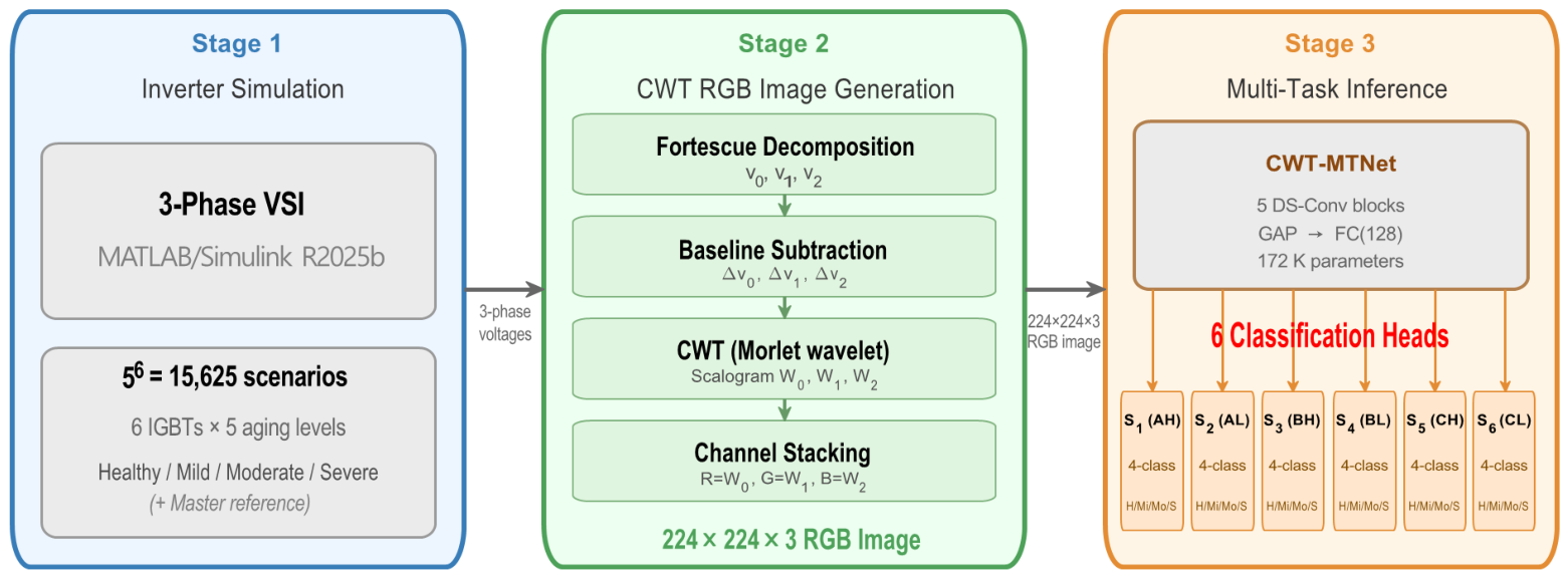
The proposed per-switch IGBT aging diagnosis system converts raw three-phase inverter voltages into per-switch aging state labels through a three-stage pipeline, illustrated in Figure 1. The design is governed by two key requirements: (i) the feature representation must preserve the joint time–frequency structure that encodes subtle Healthy–Mild distinctions, and (ii) a single forward pass must produce all six switch-level predictions without redundant per-switch inference.

Stage 1: Inverter Simulation. A three-phase two-level VSI is modeled in MATLAB/Simulink R2025b with sinusoidal PWM (SPWM) control. Each of the six IGBT switches ($S_1$–$S_6$) is parameterized by its on-state resistance $R_{\mathrm{ON}}$, which decreases monotonically under the standardized 25 °C cold-measurement convention as physical degradation advances (Section 3.2). Five discrete aging levels are assigned to each switch (

Table 2. IGBT aging state definitions.

State	${\mathit{R}}_{\mathbf{ON}}$ ($\mathbf{\Omega }$)	Class Label
Master	0.007	— (reference only)
Healthy	0.00665	1
Mild	0.00623	2
Moderate	0.00574	3
Severe	0.005	4

), and all $5^6=\mathrm{15,625}$ cross-switch state combinations are simulated. For each scenario, the steady-state three-phase output voltages $(v_a,v_b,v_c)$ are recorded as the raw signal for Stage 2. The 15,625-scenario dataset is identical to that constructed in the prior works [5,6]. Rather than idealized noise-free waveforms, the simulation embeds sensor noise directly: a zero-mean Gaussian source of variance $2.5$ is summed onto each phase voltage at the 1 MHz sampling rate ahead of the symmetrical-component decomposition. Against the measured phase RMS of 220 V (the load is rated 380 V_rms line-to-line), the resulting $\sigma =1.58$ V amounts to $0.72\%$ of the signal. The figure was verified from the recorded waveforms rather than taken from the block setting alone: the noise variance estimated from the signal-free 200–450 kHz portion of the spectrum is $2.52$, against the $2.5$ specified in the model.

Two properties of this injection govern what the results of Section 6 do and do not establish, so they are stated here rather than being left implicit. The three sources share a seed, making the injected sequence identical on all three phases, and the seed is fixed across runs, making it identical in every scenario, including the Master reference. The injection is consequently common-mode, and it cancels twice. It vanishes from $v_1$ and $v_2$ in the symmetrical-component transform, where $(1+a+a^2)/3=0$, and from $v_0$ in the Master-referenced subtraction of (1), which removes the same sequence, along with the baseline. Measured on the generated records, the residual broadband content of the three deviation channels lies 57 dB below the signal. The accuracies reported below are therefore obtained on deviation signals that are, in effect, free of sensor noise. Robustness to independent sensor noise is a distinct question, and it is measured in Section 6.9.

Stage 2: CWT RGB Image Generation. The recorded voltages are first decomposed via the Fortescue transformation into zero-sequence ($v_0$), positive-sequence ($v_1$), and negative-sequence ($v_2$) components. The deviation of each component from the Master-state baseline is computed and normalized to yield $\Delta v_k\left(t\right)$, isolating the aging-induced asymmetry while canceling load-dependent variations. A Morlet CWT is then applied to each deviation signal, producing a time–frequency scalogram that simultaneously captures transient and harmonic aging signatures at multiple frequency scales. The three scalograms are normalized by dataset-wide constants $G_k$, defined in (4), and resized to $224\times 224$ pixels, then stacked as R $={\widehat{W}}_0$, G $={\widehat{W}}_1$, B $={\widehat{W}}_2$ to form a single $224\times 224\times 3$ RGB image. This multichannel encoding preserves the physical identity of each symmetrical component while remaining fully compatible with standard RGB CNN architectures.

Stage 3: Multi-Task Inference. The RGB image is passed to CWT-MTNet as a single input. The shared backbone extracts a 128-dimensional representation capturing the global time–frequency energy distribution across all three symmetrical-component channels. Six independent classification heads then project this representation into per-switch four-class probability distributions $\{p_k^{\mathrm{H}},p_k^{\mathrm{Mi}},p_k^{\mathrm{Mo}},p_k^{\mathrm{S}}\}$ for $k=1,\dots ,6$, enabling location-specific fault identification without per-switch inference overhead.

3.2. Inverter Model, Aging States, and CWT Image Generation

Inverter Model and Aging States. The target system is a three-phase two-level VSI with six IGBTs ($S_1$–$S_6$) arranged in three half-bridge legs (upper-arm: $S_1,S_3,S_5$; lower-arm: $S_2,S_4,S_6$). SPWM with a carrier frequency of 6 kHz drives the switches; the dc-link voltage is 1000 V (split $\pm 500$ V) and the load is a balanced three-phase 50 kW, 380 V_rms, 60 Hz resistive load with an output LC filter. Each IGBT is modeled by $R_{\mathrm{ON}}$, which represents the cumulative electrical effect of bond-wire lift-off and solder-joint degradation measured at standardized 25 °C conditions. Five discrete aging levels are defined in Table 2: one Master reference state ($R_{\mathrm{ON}}=0.007\mathrm{\Omega }$) used solely for baseline subtraction, and four classifiable states spanning Healthy through Severe. The five-level reduction from 0.007 $\mathrm{\Omega }$ to 0.005 $\mathrm{\Omega }$ follows the cold-measurement convention of the benchmark, in which electrical parameters recorded under standardized 25 °C conditions shift progressively as thermo-electrical overstress accumulates [4,5].

Physical basis and scope of the $R_{\mathrm{ON}}$ model. Reviewers of power-electronic diagnosis work reasonably ask what a step in $R_{\mathrm{ON}}$ corresponds to physically, so the scope of this abstraction is stated here rather than left implicit. $R_{\mathrm{ON}}$ is used as a lumped scalar proxy for conduction-path degradation. Its justification is that the dominant wear-out mechanisms of a wire-bonded module—heel cracking and lift-off of the emitter bond wires, and fatigue of the solder layer beneath the die—all act by removing or lengthening parallel conduction paths, and therefore all present at the terminals as a change in the on-state voltage drop at a given current. That terminal quantity is what $R_{\mathrm{ON}}$ parameterizes, and it is why on-state voltage is among the most widely adopted aging precursors (Section 2).

Three boundaries of the abstraction should be stated explicitly. First, the map is not injective: a given displacement of $R_{\mathrm{ON}}$ can arise from different combinations of lifted bond wires and solder voiding, so the model resolves the severity of conduction-path degradation but not its mechanism. Second—and this is the direct answer to the question of how many bond wires a given level represents—no calibration is available in this study that would convert an $R_{\mathrm{ON}}$ level into a count of failed bond wires or a solder-crack area fraction. Establishing such a map requires a destructive analysis of accelerated-aging modules, which a simulation study cannot supply. The four classes must therefore be read as ordered severity bands on a monotonic degradation axis, not as calibrated physical damage states. Third, the direction of the shift is measured rather than assumed. Dimech and Dawson characterized eight IGBTs before and after accelerated thermo-electrical aging, recording the output characteristics at a 25 °C case temperature: after three aging iterations, the effective on-state resistance had fallen by $22.3\%$ on average and by $27.7\%$ at most, while X-ray imaging confirmed progressive die-attach voiding over the same iterations [4]. The $0.007$ to $0.005\mathrm{\Omega }$ span adopted here is a $28.6\%$ reduction, of the same order, and the convention is inherited from the benchmark on that basis [5]. This is a statement about characterization at a fixed measurement temperature, not about in-service behavior: at operating junction temperature the thermal dependence of the on-state characteristic dominates the package contribution, and the on-state voltage is instead reported to rise with degradation. The distinction does not affect the results, because the representation depends only on the magnitude of the deviation from the Master reference. The scalogram is formed from $\left|\mathcal{W}\right\{\Delta v_k\left\}\right|$, which is invariant to the sign of $\Delta v_k$, and $|R_{\mathrm{ON}}-R_{\mathrm{ON}}^{\mathrm{Master}}|$ increases monotonically across Healthy, Mild, Moderate and Severe ($0.35$, $0.77$, $1.26$ and $2.00\mathrm{m}\mathrm{\Omega }$). The class ordering, and hence everything the network is trained to discriminate, is preserved under either sign convention.

Because the pipeline is agnostic to how the deviation signals $\Delta v_k\left(t\right)$ are generated, substituting a multi-parameter electro-thermal aging model would refine the ground-truth labels while leaving the CWT-RGB encoding and the network unchanged.

CWT RGB Image Generation. Each of the 15,625 simulation scenarios produces a single $224\times 224\times 3$ CWT RGB image. The pipeline follows the symmetrical-component CWT encoding introduced in [6], with two refinements adopted here. First, because the positive- and negative-sequence deviations are complex-valued, their CWT is evaluated by linearity as $\mathcal{W}\{\Delta v_k\}=\mathcal{W}\{\Re \Delta v_k\}+j\mathcal{W}\{\Im \Delta v_k\}$, which retains both frequency half-planes rather than the positive half-plane alone. Second, the normalization constants $G_k$ are derived from a per-scenario percentile rather than a global maximum, preventing a single switching transient from setting the dataset-wide scale. Both refinements increase the usable dynamic range of the zero-sequence channel, which carries the phase-asymmetry information on which per-switch discrimination depends.

Step 1 (symmetrical-component decomposition). The three-phase output voltages are decomposed by the Fortescue transformation into zero-sequence ($v_0$), positive-sequence ($v_1$), and negative-sequence ($v_2$) components.

Step 2 (deviation signal computation). Each component is baseline-subtracted against the Master-state reference and normalized by the reference peak amplitude:

$$\begin{array}{cc}\hfill \Delta v_k\left(t\right)& ={\displaystyle \frac{v_k\left(t\right)-v_{k,\mathrm{ref}}\left(t\right)}{A_k}},\hfill \\ \hfill A_k& =\underset{t}{max}\left|v_{k,\mathrm{ref}}\left(t\right)\right|,k\in \{0,1,2\}\hfill \end{array}$$

(1)

where $v_{k,\mathrm{ref}}\left(t\right)$ is the Master-state symmetrical component. This normalization renders $\Delta v_k$ dimensionless and removes the dominant fundamental component shared by all healthy switches, isolating the aging-induced asymmetry.

Step 3 (continuous wavelet transform). The CWT of $\Delta v_k\left(t\right)$ with respect to a mother wavelet $\psi$ is defined as [51,52]:

$$W_k(\tau ,s)={\displaystyle \frac{1}{\sqrt{s}}}{\int }_{-\infty }^{\infty }\Delta v_k\left(t\right){\psi }^{*}\left({\displaystyle \frac{t-\tau }{s}}\right)dt$$

(2)

where $\tau$ is the time translation, $s>0$ is the scale (inversely proportional to frequency), and ${\psi }^{*}$ denotes the complex conjugate of the mother wavelet. This paper employs the analytic Morlet wavelet [52]:

$${\psi }_{\mathrm{M}}\left(t\right)={\pi }^{-1/4}{e}^{j{\omega }_{0}t}{e}^{-t^2/2}$$

(3)

where ${\omega }_0$ is the center angular frequency (${\omega }_0=6$ rad/s by convention [52]). The Morlet wavelet provides optimal joint time–frequency localization and is well suited to detecting the oscillatory, multi-scale energy redistributions that characterize IGBT aging signatures. The scalogram magnitude $\left|W_k\right(\tau ,s\left)\right|$ is then globally normalized and clipped to unit range:

$${\widehat{W}}_k(\tau ,s)=\min \left(\frac{|W_k(\tau ,s)|}{G_k},1\right),G_k=\underset{i\in \mathcal{D}}{max}{\mathrm{P}}_{99}\left(\left|W_k^{\left(i\right)}\right|\right)$$

(4)

where $\mathcal{D}$ is the set of 15,625 scenarios, $W_k^{\left(i\right)}$ is the channel-k scalogram of scenario i, and ${\mathrm{P}}_{99}(·)$ is the 99th percentile of the coefficient magnitudes within a single scenario. The two-stage definition is deliberate. The per-scenario percentile discards isolated switching transients that would otherwise inflate $G_k$ and render the remaining images uniformly dark, while the maximum across scenarios retains a single dataset-wide scale, so that inter-state energy differences remain encoded as brightness rather than being normalized away. For this dataset $G_0=0.00643$, $G_1=0.00160$, and $G_2=0.00156$; these constants are dimensionless because $\Delta v_k$ is already normalized by $A_k$ in (1). Coefficients exceeding $G_k$ are clipped to unity, which affects 0.10%, 0.13%, and 0.02% of pixels in the R, G, and B channels, respectively—a deliberate trade-off the low-energy regime where the Healthy and Mild states must be discriminated.

Normalization constants and data leakage. Because $G_k$ in (4) is an order statistic taken over files, computing it on the full dataset would in principle let a test scenario influence the scaling of the training images. Two facts rule this out here. First, in no channel is the maximum in (4) attained by a test-partition scenario: it comes from a training scenario for $G_0$ and $G_2$, and from a validation scenario for $G_1$, so no test file participates in the value that is actually used. Second, recomputing $G_k$ from the training partition alone ($n_{\mathrm{train}}=\mathrm{10,937}$, 70%) leaves $G_0$ and $G_2$ bit-identical and shifts $G_1$ by less than $0.01\%$—two orders of magnitude below the 8-bit quantization step ($1/255=0.39\%$) at which the images are stored, so every stored pixel is unchanged. The constants are therefore reproducible from the training split alone, and the reported accuracies are unaffected by the choice.

Step 4 (Channel stacking). The three normalized scalograms are resized to $224\times 224$ and stacked channel-wise to form the final RGB input image:

$$\mathbf{I}=\left[{\widehat{W}}_0,{\widehat{W}}_1,{\widehat{W}}_2\right]\in {[0,1]}^{224\times 224\times 3}.$$

(5)

This multichannel encoding preserves the complete joint time–frequency aging signature of all three symmetrical components in a form directly compatible with standard RGB CNN architectures.

3.3. Multi-Task Dataset

The 15,625-image dataset is labeled for the multi-task setting with one four-class label per switch per image: for switch k, the label is one of {Healthy, Mild, Moderate, Severe} (Table 2). Scenarios in which switch k is in the Master state are assigned the Healthy label, reflecting that the Master-state operation is functionally indistinguishable from Healthy at the system output level.

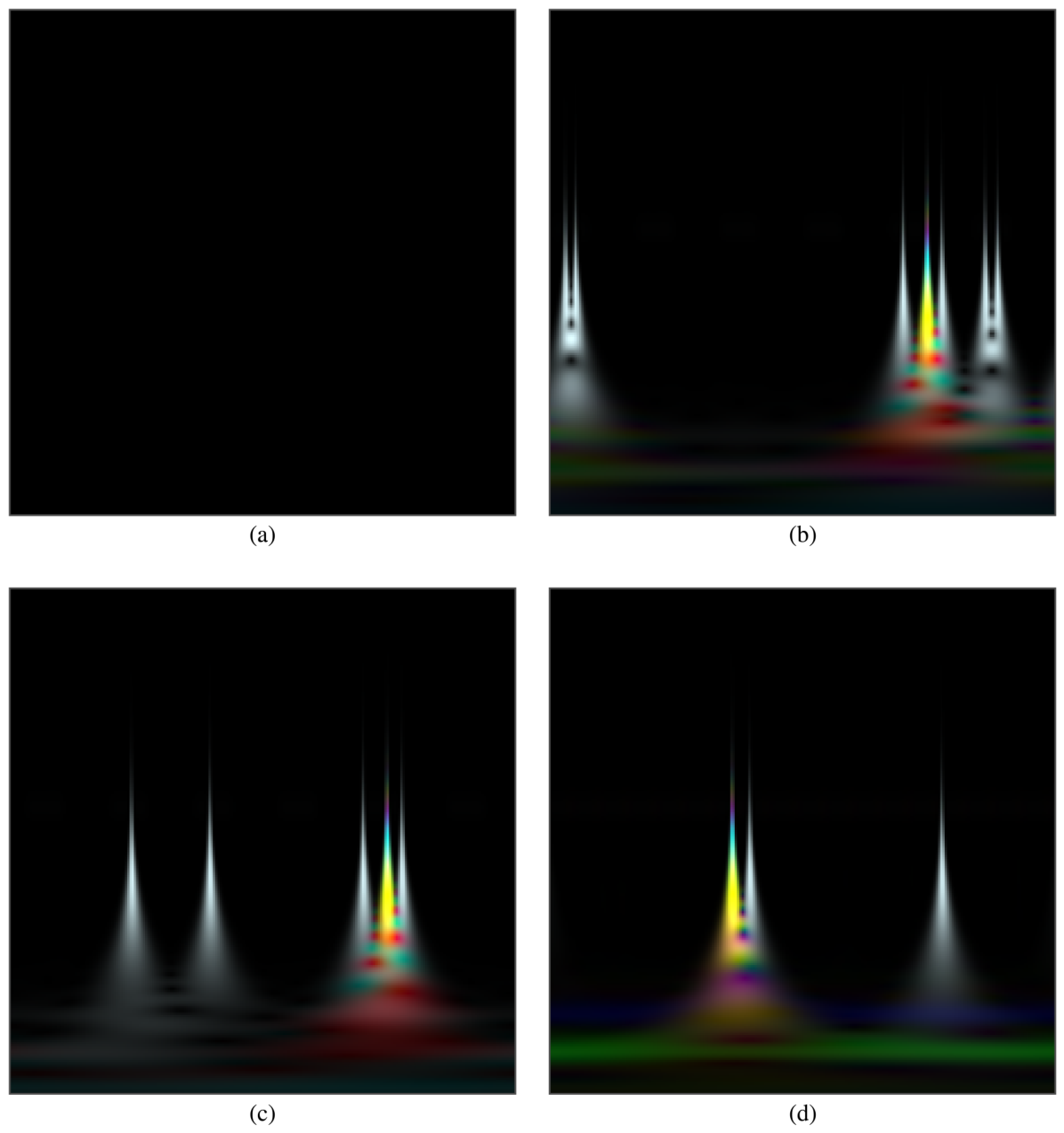
The dataset is split 70/15/15% into training (10,937), validation (2343), and test (2345) subsets using stratified sampling on the Risk Level variable with a fixed random seed (rng(49)), ensuring identical partitions across all experiments.

Table 3. Per-switch class distribution (mean over 6 switches, 15,625 images).

Class	Count (Approx.)	Ratio (%)
Healthy (incl. Master)	3125	20.0
Mild	3125	20.0
Moderate	3125	20.0
Severe	6250	40.0
Total	15,625	100.0

shows the per-switch class distribution. The Severe class is the most frequent because a single Severe device in any position contributes to multiple scenarios. Figure 2 presents four representative CWT RGB images that illustrate how switch position and aging state are encoded in the image. Figure 2a shows the near-black baseline when all switches are at Healthy/Master, confirming that the deviation signal $\Delta v_k$ is negligible under balanced operation. Figure 2b shows a bright energy spike concentrated in the upper-left time–frequency region when only $S_1$ (upper-arm, phase A) is at Severe, driven by the phase-A asymmetry in the $\Delta v_0$ R channel. Figure 2c shows the spike shift to a distinct spatial location when only $S_6$ (lower-arm, phase C) is at Severe, directly demonstrating position specificity. Figure 2d shows multiple overlapping spikes when lower-arm switches $S_2,S_4,S_6$ are simultaneously at Severe, reflecting three-phase asymmetry contributions across all channels. The spatial diversity of the CWT signatures across switch positions provides the discriminative basis for the per-switch multi-task architecture.

4. CWT-MTNet Architecture

4.1. Design Principles

CWT-MTNet is motivated by three observations from preliminary experiments:

1.

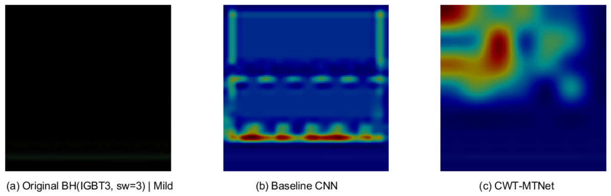
DS-Conv superiority in the CWT domain. Depthwise Separable Convolution (DS-Conv) factorizes a standard $k\times k$ convolution into a channel-wise depthwise step and a $1\times 1$ pointwise step. For CWT RGB images, this factorization is physically well suited: the R, G, B channels encode three physically distinct symmetrical components ($\Delta v_0$, $\Delta v_1$, $\Delta v_2$), so processing each channel independently in the depthwise step preserves their physical identities before cross-channel fusion in the pointwise step. In contrast, a standard $3\times 3$ convolution mixes spatial and channel information simultaneously, blurring the component-wise aging signatures from the first layer onward. Preliminary experiments confirm that MobileNet-v2 (DS-Conv) consistently outperforms standard-convolution networks on per-switch Mild recall (Section 6.2), and Grad-CAM analysis (Section 6.10) shows that DS-Conv activates distributed regions across the entire time–frequency plane, whereas standard convolution concentrates activation in narrow horizontal bands.

2.

Parameter excess in full MobileNet-v2. MobileNet-v2’s 3.7 M parameters were designed for 1000-class ImageNet recognition from natural photographic images. Its later inverted-residual blocks progressively widen the channel dimension to 320 and then 1280, capturing fine-grained texture and object detail that does not exist in CWT scalograms; on a 15,625-sample dataset with four aging classes per switch, these layers add capacity without adding discriminative content while enlarging the parameter surface over which the six heads compete. CWT-MTNet therefore retains the DS-Conv factorization and discards the late-stage width. The ablation of Section 6.6 is consistent with this choice: under the six-head operation, CWT-MTNet changes by $-2.3$ to $+2.5$ pp of Mild recall relative to its single-head counterpart—a range comparable to full MobileNet-v2 ($+0.4$ to $+3.3$ pp) and far below the standard-convolution ResNet-18 ($+25.6$ to $+42.1$ pp). The reduction does carry an accuracy cost (Section 6.4), but it is obtained at a twenty-one-fold smaller parameter budget and a ten-fold shorter CPU inference time (Section 6.5).

3.

7 × 7 feature map preserves CWT structure. Each stride-2 operation in DS-1 through DS-5 halves the spatial resolution of the $224\times 224$ input, yielding a final feature map of $7\times 7$. Each cell of this map covers a $32\times 32$ region of the scalogram. Since the ${10}^5$-sample, $0.1$ s record is resized to 224 columns, one cell spans roughly 14 ms of record time, slightly under one fundamental period at 60 Hz, together with a proportional band in the scale axis. This resolution localizes the time–frequency energy concentrations that distinguish Healthy from Mild without over-compressing spatial detail: followed by Global Average Pooling, the $7\times 7$ map accumulates a global energy summary across 49 time–frequency zones before the shared fully connected representation layer. Grad-CAM analysis (Section 6.10) confirms that this resolution enables activation to span all 49 zones, in contrast to standard convolutions that concentrate energy in narrow horizontal frequency bands. This is a design rationale rather than an optimum: the parameter study of Section 6.8 subsequently measured a 112-pixel input, which yields a $4\times 4$ final map under the same network, and found it to be the better operating point on every metric. The $7\times 7$ configuration is retained throughout for continuity with the prior studies on this benchmark, and the discrepancy is reported rather than resolved in favor of the inherited choice.

4.2. Architecture

CWT-MTNet consists of a stem convolution, five DS-Conv blocks, a shared Global Average Pooling (GAP) and fully connected (FC) layer, and six independent classification heads, as detailed in

Table 4. CWT-MTNet layer structure (input: 224 × 224 × 3). Boldface marks the summary row.

Block	Operation	Output Size	Params
Stem	Conv($3\times 3$, 32, s2) + BN + ReLU	$112\times 112\times 32$	896
DS-1	DWConv($3\times 3$, s2) + BN + ReLU6 → PWConv($1\times 1$, 64) + BN + ReLU6	$56\times 56\times 64$	2.6 K
DS-2	DWConv($3\times 3$, s2) + BN + ReLU6 → PWConv($1\times 1$, 128) + BN + ReLU6	$28\times 28\times 128$	9.3 K
DS-3	DWConv($3\times 3$) + BN + ReLU6 → PWConv($1\times 1$, 128) + BN + ReLU6	$28\times 28\times 128$	17.7 K
DS-4	DWConv($3\times 3$, s2) + BN + ReLU6 → PWConv($1\times 1$, 256) + BN + ReLU6	$14\times 14\times 256$	34.0 K
DS-5	DWConv($3\times 3$, s2) + BN + ReLU6 → PWConv($1\times 1$, 256) + BN + ReLU6	$7\times 7\times 256$	68.0 K
Shared	GAP + Dropout(0.4) + FC(128) + ReLU	128	32.9 K
Heads	6 × FC(4) + Softmax	6×4	3.1 K
Total parameters			171,672

.

Stem. A single $3\times 3$ convolution with stride 2 and 32 output channels reduces the $224\times 224\times 3$ RGB input to $112\times 112\times 32$, extracting low-level spatial features while halving the spatial resolution in a single step. Batch Normalization (BN) and ReLU are applied to stabilize and activate the stem features.

DS-Conv blocks (DS-1 through DS-5). Each block follows the depthwise-separable structure:

$$\begin{array}{cc}\hfill \mathrm{DS}\text{-}\mathrm{Block}& \left(C_{\mathrm{out}}\right)\hfill \\ \hfill & =\underset{\mathrm{spatial}}{\underbrace{{\mathrm{DWConv}}_{3\times 3}}}\to \mathrm{BN}\to \mathrm{ReLU}6\hfill \\ \hfill & \to \underset{\mathrm{channel}\mathrm{mix}}{\underbrace{{\mathrm{PWConv}}_{1\times 1}\left(C_{\mathrm{out}}\right)}}\to \mathrm{BN}\to \mathrm{ReLU}6\hfill \end{array}$$

(6)

where $\mathrm{DWConv}$ applies a $3\times 3$ filter independently per channel and $\mathrm{PWConv}$ recombines channels via $1\times 1$ convolution, reducing FLOPs by a factor of approximately 8–9. ReLU6, which clips activations at 6, is used throughout to suppress large activation values that can destabilize multi-task gradient flow. The five blocks progressively widen the channel dimension ($64\to 128\to 128\to 256\to 256$) while applying stride 2 at DS-1, DS-2, DS-4, and DS-5 to reduce spatial resolution ($112\to 56\to 28\to 28\to 14\to 7$). DS-3 retains the $28\times 28$ resolution with stride 1, deepening the frequency-band representation before the third spatial downsampling. Unlike MobileNet-v2, no inverted-residual skip connections are used; the 15,625-sample dataset does not require the deeper optimization stability that skip connections provide, and their removal further reduces parameter count.

Shared representation layer. Global Average Pooling (GAP) over the final $7\times 7\times 256$ feature map produces a 256-dimensional vector that summarizes the global time–frequency energy distribution of the input CWT image. A Dropout($p=0.4$) layer then regularizes this vector before it is projected to a 128-dimensional shared representation by $\mathrm{FC}\left(128\right)+\mathrm{ReLU}$. The 128-dimensional bottleneck acts as a shared information hub: it must capture features that are simultaneously informative for all six switch heads, implicitly encouraging the backbone to learn aging signatures that generalize across switch positions.

Six independent classification heads. Each head consists of a single $\mathrm{FC}\left(4\right)+\mathrm{Softmax}$ layer that projects the shared 128-dimensional representation to a four-class probability distribution ${\mathbf{p}}_k=[p_k^{\mathrm{H}},p_k^{\mathrm{Mi}},p_k^{\mathrm{Mo}},p_k^{\mathrm{S}}]$ for switch $k\in \{1,\dots ,6\}$. The heads are fully independent: they share no parameters and receive no inter-head information, so each produces an unbiased per-switch prediction from the common representation.

4.3. Parameter Comparison

At 171,672 parameters, CWT-MTNet is the smallest of the eleven architectures evaluated here, which span three orders of magnitude up to VGG-16 at 138.5 M; the individual counts appear in Section 6.2 and, with the corresponding storage and FLOP budgets, in Section 6.5. Five of the eleven factorize their convolutions—CWT-MTNet, MobileNet-v2, ShuffleNet, EfficientNet-B0 and NASNet-Mobile—while the Baseline CNN, SqueezeNet, GoogLeNet, ResNet-18, ResNet-50 and VGG-16 use standard convolution throughout. That split, rather than parameter count alone, is what Section 6.2 examines.

5. Training Strategy

5.1. Multi-Task Loss Function

The network produces six softmax probability vectors ${\widehat{\mathbf{y}}}_k\in {\mathbb{R}}^4$, one per switch ($k=1,\dots ,6$), where ${\widehat{y}}_{k,c}=P(\mathrm{class}c\mid \mathrm{image})$. The per-switch cross-entropy loss for a single training sample is:

$${\mathcal{L}}_{\mathrm{CE}}({\widehat{\mathbf{y}}}_k,{\mathbf{t}}_k)=-{\displaystyle \sum _{c=1}^4}{t}_{k,c}log{\widehat{y}}_{k,c}$$

(7)

where ${\mathbf{t}}_k\in {\{0,1\}}^4$ is the one-hot ground-truth label for switch k. The overall multi-task training objective is the unweighted mean of the six per-switch losses:

$${\mathcal{L}}_{\mathrm{MT}}={\displaystyle \frac{1}{6}}{\displaystyle \sum _{k=1}^6}{\mathcal{L}}_{\mathrm{CE}}({\widehat{\mathbf{y}}}_k,{\mathbf{t}}_k).$$

(8)

During backpropagation, the gradient of ${\mathcal{L}}_{\mathrm{MT}}$ with respect to the shared backbone parameters ${\theta }_{\mathrm{shared}}$ is:

$${\displaystyle \frac{\partial {\mathcal{L}}_{\mathrm{MT}}}{\partial {\theta }_{\mathrm{shared}}}}={\displaystyle \frac{1}{6}}{\displaystyle \sum _{k=1}^6}{\displaystyle \frac{\partial {\mathcal{L}}_{\mathrm{CE}}^{\left(k\right)}}{\partial {\theta }_{\mathrm{shared}}}},$$

(9)

meaning the backbone receives the averaged gradient signal from all six heads simultaneously. When these per-switch gradients point in conflicting directions, the averaged gradient may be small or misdirected—the multi-task gradient conflict quantified in Section 6.6.

Equal weighting rationale. The six heads are structurally symmetric: they share an identical label alphabet and identical class distributions (Table 3), and because aging states are drawn independently per switch across the full $5^6$ grid, no head is systematically harder than another by construction. No domain prior therefore justifies prioritizing one switch over another, and the uniform weights in (8) follow from that symmetry rather than from tuning. Adaptive schemes such as uncertainty-based task weighting [45] exist to reconcile tasks of differing scale, loss type, or noise level; with six homogeneous four-class heads sharing a single cross-entropy loss, the imbalance those schemes correct for does not arise. What equal weighting costs is measured rather than assumed. The single-head ablation of Section 6.6 retrains each architecture with a single four-class head, so that one switch owns the entire backbone and shared representation. That is the limiting case in which a task receives the largest possible share of the objective, and it therefore upper-bounds what any re-weighting of (8) could recover. For CWT-MTNet the gap is at most $2.52$ percentage points of Mild recall, and it changes sign between the two switches examined ($-2.25$ pp for BH, $+2.52$ pp for CH; Section 6.6), so the shared objective does not systematically deprive either head. By contrast, ResNet-18 loses $42.13$ pp on BH under the same comparison, which shows that the measurement is sensitive enough to expose weighting-related degradation where it exists.

5.2. Training Configuration

5.2.1. Proposed Method: CWT-MTNet (Scratch Training)

CWT-MTNet is trained from random initialization (rng(49)) for 100 epochs using the Adam optimizer with the following hyperparameters: learning rate $\eta ={10}^{-3}$, L2 weight decay $\lambda ={10}^{-4}$, mini-batch size 32, and a step learning-rate schedule that drops $\eta$ by a factor of 0.1 at epoch 40 (DropPeriod=40). Input images are normalized to $[0,1]$ via a rescale-zero-one layer; ImageNet channel statistics are deliberately not applied, because the CWT image distribution (mostly dark with sparse energy concentrations) differs fundamentally from natural photographic images (see Section 7). Mild geometric augmentation is applied to the training partition only—random horizontal reflection, rotation within $\pm {10}^{\circ }$, and isotropic scaling in $[0.9,1.1]$—as a standard regularizer against overfitting, since the training set contains 10,937 images while several of the comparison architectures carry parameter counts two to four orders of magnitude larger. The identical pipeline is applied to every architecture, every seed, and every ablation reported in this paper, and no augmentation is applied to the validation or test partitions, so all reported metrics are measured on unmodified images.

5.2.2. Comparison: Baseline CNN (Scratch Training)

The Baseline CNN (four standard Conv+BN+ReLU+MaxPool blocks, 425K parameters) is trained under the identical scratch-training protocol above—same optimizer, learning-rate schedule, normalization, and random seed—so that all performance differences between CWT-MTNet and the Baseline CNN are attributable solely to architectural choices.

5.2.3. Comparison: ImageNet-Pretrained Networks (Two-Stage Fine-Tuning)

For the six ImageNet-pretrained comparison networks (ResNet-18, ResNet-50, MobileNet-v2, VGG-16, GoogLeNet, SqueezeNet), a two-stage fine-tuning strategy is applied to avoid gradient disruption of the pretrained backbone: Stage 1 trains only the six newly appended classification heads for 10 epochs ($\eta ={10}^{-3}$) while the backbone weights are frozen, allowing the heads to stabilize before full-network optimization; Stage 2 unfreezes the entire network and continues training for 90 epochs with a reduced learning rate ($\eta ={10}^{-4}$, decayed by 0.1 at epoch 45). This two-stage protocol represents the standard practice for transfer-learning fine-tuning and is designed to give pretrained networks every opportunity to adapt to the CWT domain.

5.3. Reproducibility

The elements required to reproduce every number in this paper are collected here.

Data generation. The waveforms are produced by a Simscape three-phase two-level inverter model: split $\pm 500$ V dc link, 6 kHz SPWM carrier, balanced 50 kW/380 V_rms resistive load with an output LC filter, and a fixed-step solver at $T_s=1$µs. Each switch is a series on-state resistance taking one of the five values in Table 2, and all $5^6$ assignments are enumerated. Each run records $v_a,v_b,v_c$ over 0.1 s at 1 MHz (${10}^5+1$ samples per phase), with the independent Gaussian sensor noise of Section 3 summed onto each phase before recording.

Image generation. For each record, the Fortescue decomposition, Master-referenced deviation (1), analytic Morlet CWT, per-channel normalization (4) with the constants being stated there, and bicubic resize to $224\times 224$ are applied in that order, yielding one RGB image per scenario. The normalization constants are the only quantity computed across files; everything else is per record.

Partitioning. A single call to rng(49) precedes a per-class stratified permutation on the Risk-Level variable, split $70/15/15$. This yields 10,937 training images, 2343 validation images and 2345 test images and is re-executed identically by every training and evaluation script, so all architectures see the same partition. The multi-seed study of Section 6.4 repeats this with seeds 49–53.

Training. Adam, 100 epochs, mini-batch 32, $\eta ={10}^{-3}$ dropped by $0.1$ at epoch 40, $L_2={10}^{-4}$, shuffling every epoch, and the best-validation-loss checkpoint retained. Augmentation is as described above and applied to the training partition only. The loss is the unweighted mean of six cross-entropies, Equation (8).

Environment. MATLAB R2026a with the Deep Learning and Wavelet toolboxes; the timings reported in Section 6.5 were measured on an Intel i9-12900K CPU. The simulation model, generation scripts, trained networks and evaluation scripts are available from the author upon request, as stated in the Data Availability section.

6. Experimental Results

This section is organized as an argument rather than as a list of experiments. Section 6.1, Section 6.2 and Section 6.3 establish what the proposed network achieves and where its errors fall. Section 6.4 and Section 6.5 establish how far those numbers can be trusted and what they cost to deploy. Section 6.6 shows that the architecture, rather than the parameter budget, is what makes six-head operation viable at all. The next three then turn the question inward: Section 6.7 bounds what the input representation itself contributes, Section 6.8 measures how much its two free parameters matter, and Section 6.9 states what the pipeline requires of the acquisition front end. All three are reported as measured, including where the measurement does not favor the choices this work inherits. Section 6.10 closes by examining what the network attends to.

6.1. Pretrained vs. Scratch Training

Table 5. Pretrained (two-stage) vs. scratch training: mean accuracy (%). Boldface marks the highest value in each column.

Network	Pretrained (Two-Stage)	Scratch (100 ep)
SqueezeNet	40.14	46.48
MobileNet-v2	49.72	98.88
GoogLeNet	40.49	40.49
ResNet-18	73.72	88.50
ResNet-50	57.46	74.85
VGG-16	40.14	40.49

compares the mean accuracy (averaged over six switches) of pretrained fine-tuning (two-stage) against scratch training for three representative architectures.

Among scratch-trained networks, MobileNet-v2 achieves the highest mean accuracy (98.88%), 0.49 pp above CWT-MTNet (98.39%). This result is significant: MobileNet-v2 is a DS-Conv architecture with 3.7M parameters, and its strong scratch performance confirms that DS-Conv is well suited to the multi-task CWT domain. On this partition, CWT-MTNet leads MobileNet-v2 on Mild recall (96.73% vs. 94.88%) and on the Mild-to-Healthy misclassification rate (2.12% vs. 4.87%) at one-twenty-first the parameter count. This particular ordering should not be over-read. Seed 49 is used as the primary partition throughout Section 6.2, Section 6.3, Section 6.4, Section 6.5, Section 6.6, Section 6.7, Section 6.8, Section 6.9 and Section 6.10 for consistency with the ablation and interpretability experiments, and the five-partition study of Section 6.4 places the two networks together on Mild recall—$95.81\pm 0.82\%$ for CWT-MTNet against $95.95\pm 0.94\%$ for MobileNet-v2—so the $1.85$-point lead visible on this single draw reflects the partition rather than the models. Averaged over five partitions, MobileNet-v2 retains a $0.84$-point advantage in accuracy, and the contribution of CWT-MTNet is accordingly one of efficiency rather than of diagnostic superiority: it matches MobileNet-v2 on the safety-critical metric at a fraction of the cost. MobileNet-v2 serves as the primary quantitative comparison baseline throughout the remaining analysis.

All pretrained networks perform significantly worse than their scratch-trained counterparts. VGG-16 and GoogLeNet collapse to predicting the majority class (Healthy) under both pretrained and scratch conditions, indicative of complete failure on the minority class. These results confirm that ImageNet pretraining is detrimental for multi-task CWT diagnosis, for three reasons:

1.

Domain gap. ImageNet convolutional filters are optimized for natural image textures (edges, colors, object parts) that are structurally different from CWT time–frequency patterns. The pretrained weights bias the shared backbone toward irrelevant feature directions that are difficult to overcome with fine-tuning on only 10,937 training images.

2.

Multi-task gradient conflict. Six prediction heads generate competing gradient signals that update the shared backbone simultaneously. For large pretrained networks (11.8M–138.5M parameters), this gradient interference is amplified by the high dimensionality of the parameter space, causing the backbone to oscillate rather than converge toward a stable shared representation. The ablation study in Section 6.6 quantifies this effect directly.

3.

Parameter excess. VGG-16 (138.5M) and ResNet-50 (25.7M) contain far more parameters than can be reliably optimized on 10,937 samples. The over-parameterized network searches an excessively large weight space, and fine-tuning from pretrained initialization cannot adequately redirect it toward the CWT-specific manifold.

6.2. Scratch Training Results

Table 6. Scratch training results: mean test performance over six switches (rng = 49, 100 ep). Boldface marks the proposed network and the best value in each column.

Network	Params	Mean Acc (%)	Mean F1 (%)	Mean Mild Recall (%)	Mean Mild → Healthy (%)
CWT-MTNet (Proposed)	172 K	98.39	98.31	96.73	2.12
Baseline CNN	425 K	96.34	95.98	90.00	6.05
SqueezeNet	1.4 M	46.48	24.90	0.00	—
ShuffleNet	1.5 M	96.02	95.82	82.18	17.02
MobileNet-v2	3.7 M	98.88	98.87	94.88	4.87
EfficientNet-B0	5.4 M	96.28	96.13	83.12	15.78
NASNet-Mobile	5.5 M	94.12	93.75	74.34	24.21
GoogLeNet	7.1 M	40.49	14.41	0.00	—
ResNet-18	11.8 M	88.50	87.15	59.90	34.87
ResNet-50	25.7 M	74.85	68.13	26.45	63.93
VGG-16	138.5 M	40.49	14.41	0.00	—

presents full scratch training results for all ten comparison networks plus CWT-MTNet on the test set.

On this split, CWT-MTNet reaches a Mean Mild recall of 96.73% against 94.88% for MobileNet-v2 at a 21-fold lower parameter count; as established above and quantified in Section 6.4, that ordering does not survive averaging over partitions, and the comparison is reported here for completeness rather than as evidence of superiority.

MobileNet-v2 achieves the highest Mean Accuracy (98.88%), 0.49 pp above CWT-MTNet on this split and 0.84 pp above it across five partitions (Section 6.4)—the price CWT-MTNet pays for a twenty-one-fold smaller parameter budget. The Baseline CNN (425K, standard Conv×4) achieves 96.34% accuracy and 90.00% Mild recall, confirming that standard convolution is less effective than DS-Conv for this domain.

Recent lightweight backbones. ShuffleNet, EfficientNet-B0 and NASNet-Mobile were added to test whether the result is specific to the 2018-era comparison set. They are not competitive on this task. Their accuracies cluster near 96% (96.02, 96.28 and 94.12%), which looks unremarkable beside CWT-MTNet’s 98.39%, but the separation on Mild recall is much larger: 82.18, 83.12 and 74.34% against 96.73%, a deficit of $13.6$ to $22.4$ percentage points. The Mild-to-Healthy rate separates them further still, at 17.02, 15.78 and 24.21% against 2.12%—between seven and eleven times the rate of the proposed network in the error direction that carries the safety cost. Two explanations that suggest themselves are not supported by the numbers. The first is the architectural family: all three are separable-convolution designs—ShuffleNet uses grouped convolution with channel shuffling, EfficientNet-B0 uses inverted-residual MBConv blocks with squeeze-and-excitation, and NASNet-Mobile uses separable cells obtained by architecture search—and so is MobileNet-v2, which does not fail in this way. The second is capacity: the three do not order with parameter count, since MobileNet-v2 at 3.7 M leads ShuffleNet at 1.5 M by 12.7 percentage points of Mild recall, and EfficientNet-B0 at 5.4 M is within one point of ShuffleNet despite carrying three and a half times as many parameters. What Section 6.6 identifies as decisive is neither of these but whether an architecture tolerates six-head operation, and that measurement was not extended to the three networks added here. Their placement is therefore reported as an observation rather than explained: it adds three points to the pattern of Section 7.2, in which neither capacity nor backbone lineage predicts per-switch performance under the six-head objective. These rows are single-partition results and carry the same caveat as the others in Table 6; the five-seed treatment of Section 6.4 was not extended to them.

SqueezeNet, VGG-16, and GoogLeNet all record a Mild recall of $0\%$, but not for the same reason. VGG-16 and GoogLeNet reach exactly $40.49\%$ accuracy, the majority-class rate on this partition, so they predict a single class for every test sample; their parameter counts (138.5 M and 7.1 M) against 10,937 training images lead to optimization failure even from scratch. SqueezeNet at $46.48\%$ is above the majority-class rate and therefore does discriminate among the other states; what it loses is specifically the Healthy–Mild boundary, which its aggressive channel compression removes along with the fine-grained amplitude gradients that separate the two.

Table 7. Per-switch accuracy and Mild recall (%) under scratch training (rng = 49). The four architectures are those carried through the five-seed study of Section 6.4; the remaining comparison networks either collapse on Mild prediction or are reported in Table 6 only. Boldface marks the best value in each row within each of the two metric blocks.

	Accuracy (%)				Mild Recall (%)
Switch	Baseline	MobileNet	ResNet	CWT-	Baseline	MobileNet	ResNet	CWT-
	CNN	-v2	-18	MTNet	CNN	-v2	-18	MTNet
AH (IGBT1)	96.55	98.64	87.93	98.08	88.18	92.95	48.64	97.05
AL (IGBT2)	96.67	98.64	88.91	98.38	91.07	93.97	63.84	96.65
BH (IGBT3)	95.99	98.98	85.29	98.55	89.57	96.32	54.60	97.96
BL (IGBT4)	96.93	98.51	86.78	98.34	93.20	92.76	55.70	96.71
CH (IGBT5)	95.69	99.79	90.96	98.21	86.37	99.37	67.92	94.97
CL (IGBT6)	96.20	98.72	91.13	98.76	91.60	93.91	68.70	97.06
Mean	96.34	98.88	88.50	98.39	90.00	94.88	59.90	96.73

resolves both metrics per switch for the four architectures that the five-seed study of Section 6.4 also covers, so that the same column set carries through both. Read across the two halves, it separates the two questions the paper keeps distinct. MobileNet-v2 holds the higher accuracy on five of the six switches and on the mean, while CWT-MTNet holds the higher Mild recall on five of the six and on the mean. Accuracy and the safety-relevant metric therefore do not order the two networks the same way, which is the observation that Section 6.4 puts on a statistical footing.

Per-switch Mild recall. On seed 49, CWT-MTNet outperforms MobileNet-v2 on 5 of 6 switches; the only exception is CH (IGBT5), where MobileNet-v2 achieves 99.37% versus CWT-MTNet’s 94.97%. As noted above, this single-seed comparison favors CWT-MTNet; the multi-seed analysis (Section 6.4) provides a statistically robust characterization. CH (IGBT5) shows the lowest Mild recall for both CWT-MTNet (94.97%) and Baseline CNN (86.37%), making it the most challenging switch position for DS-Conv architectures on this dataset. For ResNet-18, AH (IGBT1) and BH (IGBT3) are the hardest switches (48.64% and 54.60%, respectively), consistent with the gradient-conflict analysis in Section 6.6.

Per-switch accuracy. CWT-MTNet achieves consistently high per-switch accuracy across all six switches (range: 98.08–98.76%, mean 98.39%), with notably lower variance than ResNet-18 (range: 85.29–91.13%, mean 88.50%). A striking finding is that the Baseline CNN (96.34% mean) substantially outperforms ResNet-18 (88.50%) in overall per-switch accuracy, despite having 28-fold fewer parameters (425 K vs. 11.8 M). This reversal directly demonstrates the cost of multi-task gradient conflict in large standard-convolution backbones: ResNet-18’s 11.8M parameters amplify inter-task gradient interference, causing the backbone to settle into a compromise representation that serves none of the six switches well. The Baseline CNN, with its limited 425 K-parameter space, experiences less interference and achieves stable per-switch accuracy (95.69–96.93%), though at the expense of a lower Mild recall ceiling. ResNet-18’s worst per-switch drops occur on BH (IGBT3) and BL (IGBT4) at 85.29% and 86.78%, consistent with the Mild recall degradation documented for the same switches in Table 7 and further quantified in the ablation study (Section 6.6).

6.3. Confusion Matrix Analysis

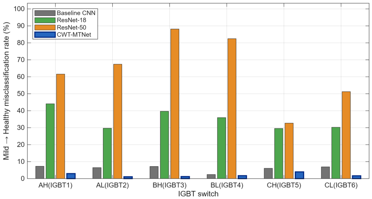
Figure 3 shows the Mild-to-Healthy misclassification rate per switch for four networks (Baseline CNN, ResNet-18, ResNet-50, and CWT-MTNet). This metric measures the fraction of Mild test samples predicted as Healthy—the most dangerous error direction, as an inverter with incipient aging is incorrectly cleared as healthy, masking the need for preventive maintenance. CWT-MTNet achieves the lowest rate across all six switches, while ResNet-50 is the most dangerous; the gap between the two is substantial at most switch positions, particularly on BH (IGBT3).

Quantitative results are shown in

Table 8. Mild-to-Healthy misclassification rate (%). Boldface marks the lowest, and therefore best, value in each row.

Switch	Baseline CNN	ResNet-18	ResNet-50	CWT-MTNet
AH (IGBT1)	7.3	44.1	61.6	3.0
AL (IGBT2)	6.5	29.7	67.4	1.1
BH (IGBT3)	7.2	39.7	88.1	1.2
BL (IGBT4)	2.4	36.0	82.5	1.8
CH (IGBT5)	6.1	29.6	32.7	4.0
CL (IGBT6)	6.9	30.3	51.3	1.7
Mean	6.05	34.87	63.93	2.12

. On this partition, CWT-MTNet achieves a mean Mild-to-Healthy rate of 2.12%, the lowest among all evaluated networks—less than half of Baseline CNN (6.05%) and an order of magnitude below ResNet-18 (34.87%). At the other extreme, ResNet-50 is the most dangerous network overall, recording a mean rate of 63.93% across the six switches; its worst case is BH (IGBT3) at 88.1%, meaning that nearly nine out of ten Mild samples on that switch are misdiagnosed as Healthy. This extreme degradation is a direct consequence of the gradient-conflict-induced collapse quantified in Section 6.6.

Misclassification direction analysis across all networks confirms that Mild errors are almost exclusively in the Healthy direction (Mild→Healthy ≫ Mild→Moderate). For CWT-MTNet, the mean Mild→Healthy rate (2.12%) is more than twice the Mild→Moderate rate (0.89%), indicating that the proposed network, like every other architecture evaluated here, carries a systematic bias toward reading Mild as Healthy. This residual asymmetric error structure—approximately one in 47 incipient-aging devices missed at fleet scale on this partition—must be accounted for in safety-critical maintenance scheduling and motivates further reduction in this error mode in future work.

6.4. Multi-Seed Statistical Validation

Single-partition results can mislead, so the four architectures that remain competitive on this task—the proposed network, the strongest lightweight baseline, the strongest general-purpose baseline, and the deepest one—were each retrained five times with independent stratified splits (seeds 49–53). Every run uses the identical scratch protocol of Section 5: He initialization with no pretrained weights, the same optimizer, schedule, epoch budget and augmentation, and the same head attachment.

Table 9. Five-seed 95% confidence intervals (seeds 49–53, $t_{0.025,4}=2.776$). All runs use an identical scratch protocol. Boldface marks the best value in each row.

Metric	CWT-MTNet	MobileNet-v2	Baseline CNN	ResNet-18
	(0.17 M)	(3.7 M)	(0.43 M)	(11.8 M)
Accuracy (%)	$98.15\pm 0.33$	$\mathbf{98}.\mathbf{99}\pm \mathbf{0}.\mathbf{13}$	$96.09\pm 0.29$	$89.93\pm 4.39$
Macro-F1 (%)	$98.07\pm 0.37$	$\mathbf{98}.\mathbf{95}\pm \mathbf{0}.\mathbf{11}$	$95.71\pm 0.32$	$88.82\pm 5.00$
Mild recall (%)	$95.81\pm 0.82$	$95.95\pm 0.94$	$89.22\pm 0.80$	$64.34\pm 12.45$
Mild→Healthy (%)	$\mathbf{2}.\mathbf{77}\pm \mathbf{0}.\mathbf{51}$	$3.74\pm 1.08$	$6.52\pm 0.68$	$30.37\pm 9.79$

reports 95% confidence intervals ($t_{0.025,4}=2.776$, $n=5$).

Three readings follow.

The proposed network is close to MobileNet-v2 and level with it on the safety-critical metric. MobileNet-v2 retains a mean accuracy advantage, but it is $0.84$ percentage points at $21\times$ the parameter count. On Mild recall—the quantity that governs whether incipient degradation is detected at all—the two are statistically indistinguishable, $95.81\pm 0.82\%$ against $95.95\pm 0.94\%$, with heavily overlapping intervals. CWT-MTNet additionally records the lowest Mild-to-Healthy rate of the four, $2.77\pm 0.51\%$ against $3.74\pm 1.08\%$.

Depth without a suitable inductive bias is unstable under the six-head objective. ResNet-18 does not merely perform worse; its Mild-recall interval spans $\pm 12.45$ percentage points, fifteen times wider than CWT-MTNet’s $\pm 0.82$, and its per-seed values range from $56.18\%$ to $81.77\%$. Its Mild-to-Healthy rate, $30.37\pm 9.79\%$, means that, on an unfavorable partition, roughly two in five incipiently aged devices are reported healthy. This is the same failure that Section 6.6 isolates as multi-task gradient conflict, and the seed spread shows it is systematic rather than an artifact of one draw.

Consistency separates the two lightweight designs. The Baseline CNN is stable ($\pm 0.29$ on accuracy) but sits $2.1$ points below CWT-MTNet in accuracy and $6.6$ points below in Mild recall, with 2.5× the parameters. Narrow intervals are therefore not purchased by capacity: among the four, the two designs with the tightest Mild-recall intervals are the smallest and the depthwise-separable one.

6.5. Deployment Cost

Table 10. Deployment Cost (224 × 224, Batch = 1, CPU: Intel i9-12900K). Boldface marks the proposed network, which is the lowest-cost entry on every one of the four metrics.

Network	Params	FLOPs	Size	CPU
	(M)	(G)	(MB)	(ms/img)
CWT-MTNet (Ours)	0.172	0.098	0.7	3.1 ± 0.4
Baseline CNN	0.425	0.103	1.7	3.9 ± 0.6
SqueezeNet	1.367	0.380	5.5	5.0 ± 0.6
MobileNet-v2	3.653	0.300	14.6	32.4 ± 1.5
GoogLeNet	7.130	1.500	28.5	139.4 ± 4.7
ResNet-18	11.826	1.814	47.3	100.4 ± 2.6
ResNet-50	25.715	4.089	102.9	142.9 ± 3.5
VGG-16	138.49	15.470	554.0	40.7 ± 0.7
FLOPs: literature values; CWT-MTNet/CNN: analytical. Latency: median ± std over 45 runs after 5 warm-up.

compares deployment cost for all evaluated architectures, measured on an Intel Core i9-12900K CPU with a single-image batch.

CWT-MTNet is the most efficient architecture across all four cost dimensions: fewest parameters (0.172 M), smallest model size (0.7 MB), lowest FLOPs (0.098 G), and fastest CPU inference (3.1 ms/image). Compared to MobileNet-v2 it is 21× lighter, 21× smaller in storage, and 10.4× faster.

Which cost actually binds. Latency is not the binding constraint for this application, and the reason is stated here rather than left implicit. Bond-wire and solder-layer fatigue evolve over thousands of operating hours, so aging diagnosis does not reside within the switching-frequency control loop. It is a periodic health check, invoked at a maintenance-relevant cadence—hourly, daily, or at service intervals—on a recorded window of 0.1 s. A pipeline that returns an answer in seconds is therefore already orders of magnitude faster than the process it observes, and further reduction in latency confers no practical benefit. Accordingly, the latencies in Table 10 are reported to characterize the classifier, not as evidence of real-time capability. They time the network forward pass alone, on a desktop CPU, at batch size one; the CWT stage that produces the input image is not included and would dominate the end-to-end time, since each diagnosis requires three scalograms of a ${10}^5$-sample record.

The binding constraint is memory. A production inverter controller runs its existing control firmware on a fixed part, and a diagnostic model is deployable only if it fits in the memory already present on that part: a model that forces a controller upgrade will not be adopted, however quickly it runs. This is the sense in which the 21-fold reduction matters. At 0.7 MB—0.17 MB under int8 quantization, the four-fold saving that weight-only 8-bit conversion reliably delivers for convolutional networks of this size [53]—CWT-MTNet is within the on-chip RAM of the DSP-class microcontrollers used in industrial drives, whereas MobileNet-v2 at 14.6 MB is not, and the gap is one of kind rather than degree. That is an argument from footprint, and it is the full extent of the deployment claim made here: no implementation on an embedded target was carried out, and porting the transform stage—most plausibly as a fixed filter bank evaluated incrementally rather than as a full offline CWT—remains future work.

6.6. Ablation Study: Gradient Conflict Quantification

To directly quantify the effect of multi-task gradient conflict, a single-head (SH) baseline was trained for each combination of network and target switch, keeping the backbone and shared FC(128) identical to the multi-task (MT) model and replacing the six four-class heads with one head targeting the switch of interest. The SH model minimizes ${\mathcal{L}}_{\mathrm{CE}}({\widehat{\mathbf{y}}}_k,{\mathbf{t}}_k)$ for a single switch, k, while the MT model minimizes Equation (8). All hyperparameters are identical (rng=49, 100 ep, $\eta ={10}^{-3}$, L2 $={10}^{-4}$).

The results for BH (IGBT3) and CH (IGBT5) are shown in

Table 11. Single-Head vs. Multi-Task Mild recall (%): ablation study. SH = single-head model trained for one switch; MT = the six-head multi-task model of Table 7 evaluated on that switch; ${\Delta }_{\mathrm{SH}}$ = SH − MT (positive = SH advantage over MT). Boldface marks the largest degradation under multi-task operation, not the best performance.

Network	BH (IGBT3)			CH (IGBT5)
	SH (%)	MT (%)	${\Delta }_{\mathrm{SH}}$(pp)	SH (%)	MT (%)	${\Delta }_{\mathrm{SH}}$(pp)
Baseline CNN	90.39	89.57	$+0.82$	93.29	86.37	$+6.92$
ResNet-18	96.73	54.60	+42.13	93.50	67.92	+25.58
MobileNet-v2	99.59	96.32	$+3.27$	99.79	99.37	$+0.42$
CWT-MTNet	95.71	97.96	$-2.25$	97.48	94.97	$+2.52$

; these two switches were selected because they bracket the range of per-switch difficulty, although which of them is the harder depends on the architecture (Section 6.3).

The results reveal four distinct behavioral categories:

1.

Baseline CNN: mild SH advantage. The SH model outperforms the MT model by +0.82 pp (BH) and +6.92 pp (CH). The compact standard-convolution backbone (425K parameters) is more resistant to gradient conflict than ResNet-18 because its limited parameter space reduces the degrees of freedom for conflicting gradients to interfere.

2.

ResNet-18: severe gradient conflict. When trained as a dedicated single-switch network (SH), ResNet-18 achieves 96.73% Mild recall on BH, demonstrating sufficient capacity for the per-switch diagnosis task. In the multi-task setting (MT), however, this drops to 54.60%: SH outperforms MT by +42.13 pp, confirming that gradient conflict—not insufficient network capacity—is the limiting factor. The Mild-to-Healthy rate on BH rises from 1.43% (SH) to 39.67% (MT)—a 28-fold increase—further underscoring the safety risk of gradient-conflict-induced collapse in this backbone.

3.

MobileNet-v2: robust to gradient conflict. The SH advantage is only +3.27 pp (BH) and +0.42 pp (CH). The factored DS-Conv structure induces implicit gradient regularization: because depthwise and pointwise filters occupy different parameter subspaces, task-specific gradients are partially decoupled in the parameter update, reducing direct interference in the shared representation.

4.

CWT-MTNet: no systematic multi-task penalty. CWT-MTNet is the only network whose ${\Delta }_{\mathrm{SH}}$ changes sign between the two switches: $-2.25$ pp on BH, where the six-head model is the better of the two, and $+2.52$ pp on CH. Neither magnitude approaches the ResNet-18 collapse, and the inconsistent direction indicates that no systematic gradient conflict is present at this scale. A plausible reading is that with 172 K parameters the six correlated switch objectives act as a regularizer on the shared representation rather than as competing demands on it, although the present two-switch experiment cannot separate this explanation from ordinary run-to-run variation.

6.7. What the Representation Contributes

The CWT-RGB encoding is inherited from the prior studies on this benchmark rather than proposed here (Section 2), so its contribution must be established rather than assumed. This subsection does so by holding the signal fixed and varying only the encoding.

Protocol. All three variants receive the same Master-referenced deviations $\Delta v_0$, $\Delta v_1$, $\Delta v_2$ and differ only in how those signals are encoded before the network:

1.

Phase preserved, no decomposition. The deviations enter a 1-D network directly as five real channels ($\Re \Delta v_0$, $\Re \Delta v_1$, $\Im \Delta v_1$, $\Re \Delta v_2$, $\Im \Delta v_2$).

2.

Phase discarded, no decomposition. The same signals are reduced to magnitude—$|\Delta v_0|$ as its analytic envelope, together with $|\Delta v_1|$ and $|\Delta v_2|$—matching the magnitude-only construction of the image channels.

3.

Phase discarded, CWT decomposition. The proposed pipeline: $\left|\mathcal{W}\right\{\Delta v_k\left\}\right|$ normalized by (4), quantized to 8 bits and resized to $224\times 224$.

The 1-D network is the exact counterpart of CWT-MTNet: identical block count, channel widths $[64,128,128,256,256]$, strides $[2,2,1,2,2]$, global average pooling, shared FC(128) and six heads, with $[k\times 1]$ kernels in place of $[k\times k]$. Parameter counts therefore land within $2.3\%$ of one another, so the comparison is not confounded by capacity. This control is not a weakened alternative: one-dimensional convolutional networks applied directly to sampled converter waveforms are an established alternative to time–frequency imaging in this field [33], and the depthwise-separable factorization used here transfers to the one-dimensional case without modification [48]. The comparison therefore places the proposed encoding against a design that a practitioner might reasonably choose instead. Split, seed, optimizer, schedule and epoch budget are those of Section 5; the 1-D variants use the natural counterpart of the image augmentation, a random circular time shift with amplitude scaling. Before entering the 1-D networks the deviations are low-pass filtered at 25 kHz and decimated $20:1$, which is lossless in practice: Section 6.9 measures the deviation content above 100 kHz at 57 dB below the signal.

The encoding decomposes into two separable costs. Discarding phase costs $3.97$ percentage points within the time domain ($100.00\to 96.03\%$). Applying the CWT then returns $2.36$ of them ($96.03\to 98.39\%$). The second figure is the one that bears on the proposed pipeline: once phase has been discarded, the time–frequency decomposition is not neutral but recovers most of what magnitude-only encoding gives up.

The mechanism is measurable rather than conjectural. Taking the magnitude of the raw deviation collapses each channel to a single envelope and destroys the distribution of energy over frequency, whereas taking $\left|\mathcal{W}\right|$ preserves magnitude at every time–scale pair. The clearest symptom is redundancy. Because the phase voltages are real, $\Delta v_2=\overline{\Delta v_1}$, so the raw magnitudes satisfy $|\Delta v_2|=|\Delta v_1|$ exactly—the measured correlation is $+1.000000$—and the third channel carries nothing. The corresponding image channels are formed as $|\mathcal{W}\{\Re \Delta v_k\}+j\mathcal{W}\{\Im \Delta v_k\}|$ and are not equal because the wavelet transforms of the real and imaginary parts are themselves complex. The decomposition therefore retains structure that raw magnitude cannot.

Uniformity is the larger practical difference. The mean conceals the more relevant behavior. Per-switch accuracy under magnitude-only encoding ranges over $8.40$ percentage points, from $91.60\%$ on AL (IGBT2) to $100.00\%$ on BL (IGBT4); under the CWT encoding, the same spread is $0.68$ points, twelve times tighter. A diagnostic system has no prior knowledge of which of the six devices has aged, so consistency across positions is as material as the mean.

What this does not establish. The first row of

Table 12. What the encoding costs. All variants receive the same deviation signals and differ only in how those signals are encoded. SD and range are taken across the six per-switch accuracies. Boldface marks the encoding adopted in this paper, not the best value in each column: the phase-preserving variant in the first row is more accurate.

Encoding	Params	Acc.	Macro-F1	Mild	Mild → H	SD	Range
		(%)	(%)	(%)	(%)	(pp)	(pp)
Phase preserved, no CWT	168,280	100.00	100.00	100.00	0.00	0.00	0.00
Phase discarded, no CWT	167,832	96.03	95.66	95.78	1.53	3.46	8.40
Phase discarded, CWT	171,672	98.39	98.31	96.73	2.12	0.24	0.68

is an upper reference rather than a competing method, since it uses information the representation discards by construction. It is nevertheless the best result in the table, and this is stated explicitly. Two further measurements bound how much weight the comparison can carry. First, the task is very nearly a linear inverse problem: an ordinary least-squares probe on 201 time samples per channel, with no learning at all, classifies the six switches at $99.96\%$, while the same probe on permuted labels returns $20.84\%$ against a majority-class rate of $40.49\%$. The high absolute numbers are a property of a deterministic and effectively noise-free benchmark (Section 6.9), not of the classifier. Second, the ordering does not survive contact with independent sensor noise: every encoding falls below $53\%$ once noise is injected at $0.5\%$ of the phase RMS (Section 6.9), so robustness does not separate them either.

The honest summary is therefore narrow. On this benchmark, the CWT decomposition is not a necessary condition for per-switch diagnosis, and a phase-preserving 1-D network on the same signals is more accurate. What the decomposition demonstrably provides, given that phase has been discarded, is a $2.36$-point recovery and a twelvefold improvement in cross-switch consistency. Retaining phase in the time–frequency domain—for instance, by encoding the real and imaginary scalograms as separate channels rather than their magnitude—follows directly from the first row of Table 12 and is the most concrete extension this analysis suggests.

6.8. Sensitivity to the CWT Parameters

Section 6.7 asked whether the decomposition helps at all. This subsection addresses the narrower question that follows from a positive answer: the extent to which the two free parameters of that decomposition—the mother wavelet and the output resolution—affect the outcome.

Protocol. Image sets were regenerated for three mother wavelets (analytic Morlet, bump, and Morse) at two resolutions ($224\times 224$ and $112\times 112$), holding every other stage of Section 3 fixed. Because a change of wavelet changes the scale of the coefficients, the normalization constants of (4) were re-derived per wavelet by the same two-stage operator, giving $(G_0,G_1,G_2)$ of $(0.00644,0.00160,0.00156)$ for Morlet, $(0.00334,0.00093,0.00080)$ for bump and $(0.00542,0.00142,0.00134)$ for Morse; no wavelet is therefore penalized by a mismatched scale. CWT-MTNet was then trained on each set under the protocol of Section 5, and

Table 13. Sensitivity of CWT-MTNet to the mother wavelet and the output resolution. Same network, split, seed and training protocol throughout; $\mathrm{171,672}$ parameters in every row. Single seed. Boldface marks the best value in each column.

Wavelet	Resolution	Accuracy	Macro-F1	Mild	Mild → H
		(%)	(%)	(%)	(%)
Morlet (deployed)	224	98.39	98.31	96.73	2.12
Morlet (control)	224	98.49	98.43	95.53	3.18
Morlet	$\mathbf{112}$	99.59	99.57	98.72	0.91
Morse	224	97.25	97.06	93.79	3.61
Bump	224	93.85	93.36	87.37	7.98

reports the outcome. The network is unchanged across all rows—global average pooling absorbs the spatial size, so the parameter count is $\mathrm{171,672}$ at both resolutions and the resolution comparison is not confounded by capacity.

The Morlet, 224-pixel set is a control: it is a regeneration of the deployed images through the same code path. Sampled over 100 scenarios, its pixels differ from the deployed set by at most one gray level (mean $0.0003$ on the 0–255 scale), and training on it reproduces the deployed accuracy to within $0.10$ percentage points. The reconstruction is therefore exact enough for the remaining rows to be read against it.

The mother wavelet matters, and the inherited choice is the best of the three. At equal resolution, the analytic Morlet leads Morse by $1.24$ percentage points and bump by $4.64$, with the same ordering on Mild recall ($95.53$, $93.79$, $87.37\%$) and the reverse ordering on Mild-to-Healthy ($3.18$, $3.61$, $7.98\%$). The spread is larger than the seed-to-seed variation of Section 6.4 ($\pm 0.33$ on accuracy), so it is not noise. The ranking is consistent with the time–frequency trade-off each wavelet makes: the bump wavelet is the most compact in frequency and correspondingly the poorest at localizing the switching-band transients in time, which Section 6.7 identifies as where the aging signature lives.

Halving the resolution improves accuracy and reduces cost. The 112-pixel Morlet set is the best row of Table 13 on every metric—$99.59\%$ accuracy against $98.49$, Mild recall $98.72$ against $95.53$, and a Mild-to-Healthy rate of $0.91\%$, the lowest recorded anywhere in this work—while the convolutional cost scales with spatial area and therefore falls by roughly a factor of four. The likely reason is that the scalogram is smooth relative to a $224\times 224$ grid: resizing to 112 discards sampling redundancy rather than signal, and the resulting network sees a $4\times 4$ final feature map instead of $7\times 7$, which aggregates more strongly before the shared representation.

This result is reported as measured rather than adopted. Each row is a single training run, and the $1.10$-point resolution gap exceeds the $\pm 0.33$ seed interval of Section 6.4; confirming it would therefore require the same five-seed treatment applied to the architectures. The remaining experiments in this paper use the 224-pixel configuration for continuity with the prior studies on this benchmark; the measurement above indicates that a 112-pixel front end is the more efficient operating point and is the first change a deployment should consider.

6.9. Measurement-Noise Robustness

Section 3 established that the noise embedded in the dataset is common-mode and cancels in the deviation channels. This subsection removes that convenience and measures what the network does when each voltage sensor contributes its own independent broadband noise.

Protocol. Zero-mean Gaussian noise of standard deviation $\sigma =p{v}_{\mathrm{rms}}$ is added independently to $v_a$, $v_b$ and $v_c$ before the Fortescue decomposition, with a fixed realization per file so that levels are compared on paired samples. Images are regenerated through the identical pipeline of Section 3 using the deployed constants $G_k$, which are held fixed because a commissioned front end does not recalibrate itself when its environment changes. The network is not retrained and never sees a noisy image. The $p=0$ row is regenerated through this same code path rather than read from the clean image set, and it reproduces the published accuracy to thirteen significant figures; it therefore validates the pipeline reconstruction and makes every other row commensurable with it.

Result.

Table 14. Degradation of the deployed network under independent sensor noise. No retraining; p is the injected standard deviation as a fraction of the phase RMS. Boldface marks the noise-free reference row against which the remaining rows are read.

p (%)	Accuracy (%)	Macro-F1 (%)	Mild Recall (%)	Mild → Healthy (%)
0	98.39	98.31	96.73	2.12
0.5	41.76	29.13	14.10	56.98
1	43.20	33.42	13.23	55.46
2	34.71	26.23	6.51	45.42
3	32.01	23.76	5.33	43.23
5	29.56	21.12	3.87	41.09
10	28.33	19.40	5.09	36.69

does not describe a graded degradation but an abrupt collapse. Accuracy falls from $98.39\%$ to $41.76\%$ at $p=0.5\%$ and is essentially flat thereafter; Mild recall, the quantity that matters for early detection, falls from $96.73\%$ to $14.10\%$ and the Mild-to-Healthy rate rises from $2.12\%$ to $56.98\%$. The near-constancy of the rows beyond $p=0.5\%$ shows that the failure is not a gradual loss of discriminability but the loss of the representation itself.

The reason is a scale mismatch, and it is measurable rather than speculative. On the recorded waveforms, the aging-induced deviation of the phase voltage has an RMS of $0.187$ V, whereas $p=0.5\%$ of the phase RMS is $1.10$ V. The perturbation exceeds the signature it is meant to leave intact by a factor of $5.9$, and, unlike the simulation’s common-mode noise, it survives both the symmetrical-component transform and the baseline subtraction.

Recovery by a band-limited front end. A real acquisition chain does not present raw 1 MHz broadband noise to a classifier; it band-limits first. Since white noise is spread to the Nyquist frequency while the aging signature is not, a low-pass at $f_c$ suppresses the noise amplitude by $\sqrt{(f_s/2)/f_c}$ while, in principle, leaving the signature untouched. The filter was therefore placed ahead of the decomposition, applied to the baseline as well so that the deviation stays consistently defined, and the sweep repeated with the same network and the same noise realizations (

Table 15. Effect of a low-pass front end. Suppression is the theoretical white-noise amplitude reduction $\sqrt{(f_s/2)/f_c}$. Same network, no retraining.

Front End	Suppression	$\mathit{p}=0$		$\mathit{p}=0.5\%$
		Acc. (%)	Mild (%)	Acc. (%)	Mild (%)
None	1.0×	98.39	96.73	41.76	14.10
Low-pass 20 kHz	5.0×	98.29	96.37	48.48	17.10
Low-pass 5 kHz	10.0×	32.57	33.20	29.95	16.63

).

Three readings follow, and together, they close the question. First, the filter itself is harmless: at 20 kHz the noise-free control loses $0.10$ percentage points ($98.39\to 98.29\%$), confirming that the deviation carries almost no energy above that frequency and that no retraining is needed to accommodate the front end. Second, the aging signature lives in the switching band: moving the cutoff to 5 kHz, below the 6 kHz carrier, collapses the noise-free control to $32.57\%$—barely above the $25\%$ that four balanced classes give by chance. What was removed was not noise but signal. Third, the suppression actually required is larger than either setting provides: placing the noise 10 dB below the signature demands a factor of $18.7$, hence $f_c\approx 1.4$ kHz, which is below the carrier and therefore inside the band the second reading shows to be indispensable.

The two requirements are thus incompatible. A cutoff high enough to preserve the signature ($\ge 20$ kHz) suppresses too little, and a cutoff that suppresses enough ($\le 1.4$ kHz) removes the signature. No low-pass front end resolves this, and the $48.48\%$ obtained at 20 kHz is the best such a filter can do.

The collapse is not specific to the image encoding. Because the failure is one of scale rather than of model class, it should affect any encoding of the same deviation signals. This was checked directly. The two 1-D networks of Section 6.7 were evaluated on the same noise realizations, again without retraining (

Table 16. Independent sensor noise degrades every encoding of the same deviation signals. No retraining; identical noise realizations across rows and columns. Mean accuracy over the six switches (%). Effective SNR is quoted at the phase voltage and combines the simulation’s inherent common-mode noise ($\sigma =1.58$ V) with the injected independent noise; the $p=0$ row is the inherent noise alone, which cancels in the deviation channels (Section 3.2) and therefore does not reach the classifier.

Added Noise	Effective SNR	Phase Preserved	Phase Discarded	Phase Discarded
p (%)	(dB)	No CWT	No CWT	CWT (Proposed)
0.0	42.9	100.00	96.03	98.39
0.5	41.1	52.43	30.14	41.76
1.0	38.2	41.98	26.33	43.20
2.0	33.5	33.03	26.60	34.71
5.0	25.9	30.85	27.96	29.56
10.0	20.0	30.19	27.48	28.33

). Every encoding falls from its noise-free value to below $53\%$ at $p=0.5\%$ and to the high twenties beyond $p=2\%$. Preserving phase does not help—the phase-preserving network is the most accurate at $p=0$ and remains within a few points of the others thereafter—and discarding it does not help either. Robustness therefore does not distinguish the encodings, and the front-end requirement derived above applies to all of them.

What the pipeline does require. The remedy is not selectivity in frequency but coherent averaging in time. Estimating $v_0$, $v_1$ and $v_2$ by DFT or averaged phasor extraction over one fundamental period—the front-end standard in frequency-domain inverter diagnosis—averages $16,667$ samples at the 1 MHz rate and suppresses white noise by $\sqrt{16,667}\approx 129$. That returns the $p=0.5\%$ perturbation from $1.10$ V to $8.5$ mV, or $26.8$ dB below the $0.187$ V signature, with margin to spare. The representation proposed here is therefore not robust to raw broadband noise on its own; it presupposes such a front end, and the experiments above quantify how much suppression that the front end has to deliver rather than assuming it is sufficient.

Scope of these measurements. Two limits should be read with the numbers. The low-pass is realized as an ideal spectral truncation, so Table 15 reports the best a filter of that cutoff could achieve, not what a realizable analog filter would. In addition, the $0.1$ s records span six fundamental periods, so the $129\times$ suppression of full-period phasor estimation cannot be demonstrated on this dataset without collapsing the time axis the scalogram requires; establishing it experimentally needs longer records and is left to future work.

6.10. Grad-CAM Analysis

The ablation study established that CWT-MTNet is robust to multi-task gradient conflict, but it did not explain why DS-Conv-based architectures better separate the Healthy and Mild aging states. The accuracy gap (Baseline CNN: 90.00% Mild recall; CWT-MTNet: 96.73%) raises an interpretability question: whether the two architectures attend to different time–frequency regions, and whether that difference accounts for the diagnostic gap. Grad-CAM [50] is applied here to resolve this question by visualizing which regions of the CWT RGB image each architecture attends to when predicting Healthy vs. Mild. This analysis serves two purposes: (i) to validate that CWT-MTNet focuses on physically meaningful time–frequency energy patterns rather than spurious correlations, and (ii) to provide a visual explanation for the Healthy–Mild discrimination advantage. Baseline CNN and CWT-MTNet are compared on the same BH (IGBT3) test images, with heatmaps computed at the final convolutional layer (relu4 for Baseline CNN; the DS-5 block output for CWT-MTNet), which provides the highest-level spatial features before GAP.

Figure 4 shows Grad-CAM overlays for a BH (IGBT3) Mild test sample: the original CWT image (a), the Baseline CNN activation map (b), and the CWT-MTNet activation map (c).

As shown in Figure 4b, Baseline CNN consistently activates a narrow horizontal band in the mid-frequency range of the scalogram. For both Healthy and Mild test samples, the activated region is nearly identical, reflecting that the standard Conv × 4 backbone’s limited receptive field captures only local frequency bands rather than the global time–frequency energy distribution that differentiates Mild from Healthy. In misclassified Mild samples, the Baseline CNN produces a Healthy-identical activation map, confirming that the misclassification arises from an inability to detect the subtle distributed energy shifts introduced by early aging.

CWT-MTNet activates a wider, more spatially distributed region of the scalogram for both classes, with clearly different activation patterns for Healthy versus Mild. The distributed activation arises because DS-Conv applies independent filters per channel across the full spatial extent of the feature map before mixing channels via $1\times 1$ convolution, enabling the network to encode both local frequency patterns and global time–frequency energy distribution. This global encoding is precisely the information that distinguishes Mild from Healthy in the CWT scalogram: Mild-state aging introduces subtle energy redistribution across multiple frequency bands and time windows simultaneously, which a narrow-band detector inevitably misses.

7. Discussion

7.1. Why DS-Conv Outperforms Standard Convolution in CWT Domain

The Grad-CAM evidence points to a fundamental mismatch between standard convolution and the structural properties of CWT scalograms. A standard $3\times 3$ convolutional filter has a local receptive field that, after four pooling stages, covers only a $48\times 48$ region of the $224\times 224$ input. CWT aging signatures, however, are non-local: Mild aging causes distributed energy redistribution across many frequency bands and time windows simultaneously. DS-Conv addresses this by separating spatial and channel mixing: the depthwise $3\times 3$ filter captures local spatial structure independently per channel, while the $1\times 1$ pointwise filter aggregates cross-channel information globally. After five DS-Conv blocks with progressively growing receptive fields, the network accumulates global time–frequency context that standard convolution requires much deeper architectures to achieve.

7.2. CWT-MTNet vs. MobileNet-v2: Efficiency and Stability

The multi-seed experiment (Table 9) separates the lightweight designs from the deep baseline far more sharply than any single partition does. Averaged over five splits, MobileNet-v2 holds a $0.84$-point accuracy advantage over CWT-MTNet ($98.99\pm 0.13$ against $98.15\pm 0.33\%$), consistent with its $21\times$ larger capacity. On Mild recall—the metric that decides whether incipient degradation is seen at all—the two are indistinguishable: $95.95\pm 0.94\%$ against $95.81\pm 0.82\%$, with intervals that overlap almost entirely. Of the two, CWT-MTNet records the lower Mild-to-Healthy rate, $2.77\pm 0.51$ against $3.74\pm 1.08\%$.

Stability is where the architectures genuinely diverge, and the divide does not fall between the two DS-Conv networks. Both hold their Mild-recall intervals below one percentage point, as does the Baseline CNN ($\pm 0.80$); ResNet-18 spans $\pm 12.45$, with per-seed values running from $56.18\%$ to $81.77\%$. Capacity therefore confers neither accuracy nor predictability under the six-head objective: the three smallest networks in the comparison are also the three most repeatable, and the largest is by a wide margin the least.

The practical reading is that CWT-MTNet concedes little and gains much. It gives up $0.84$ accuracy points to a model $21\times$ its size, matches that model where safety is concerned, and is an order of magnitude more predictable than a model $69\times$ its size—a useful combination where the training set is fixed by available historical records, cannot be resampled, and where an unfavorable partition cannot be identified in advance.

The deployment cost comparison (Table 10) quantifies the efficiency advantage: CWT-MTNet is 21× lighter (0.172 M vs. 3.653 M), 21× smaller in storage (0.7 MB vs. 14.6 MB), and 10.4× faster on CPU (3.1 ms vs. 32.4 ms per image). MobileNet-v2’s later inverted-residual blocks, which account for approximately 70% of its parameters, encode image-level features suited to 1,000-class natural image classification but unnecessary for the 4-class per-switch aging diagnosis task. CWT-MTNet’s five DS-blocks, purpose-designed for $224\times 224$ CWT inputs, reach a $7\times 7$ final spatial resolution that matches the effective frequency–time scale of the aging signatures without overparameterizing later stages. At 0.7 MB—0.17 MB under int8 quantization—CWT-MTNet’s static footprint is within the on-chip RAM of the DSP-class microcontrollers used in industrial inverter control units, so per-switch diagnosis can run alongside the existing control firmware rather than requiring a controller upgrade or an offboard edge server. As set out in Section 6.5, the binding constraint for a slow-timescale diagnostic task is memory rather than speed; the transform stage has not been ported to an embedded target and no on-target measurement was made.

7.3. Why Scratch Training Outperforms ImageNet Pretraining on CWT Images

The consistent superiority of scratch-trained networks over ImageNet-pretrained networks in this domain can be attributed to three compounding mechanisms.

(1) Input distribution mismatch. ImageNet-pretrained networks apply per-channel normalization using the statistics of the ImageNet-1K benchmark [54]: mean ${\mu }_{\mathrm{IN}}\approx [0.485,0.456,0.406]$ and standard deviation ${\sigma }_{\mathrm{IN}}\approx [0.229,0.224,0.225]$. CWT RGB images, however, are structurally sparse: the 99th-percentile normalization in Stage 2 ensures that most pixels across the 15,625-scenario dataset lie close to zero, with high-energy values concentrated in a small fraction of the image. When a CWT pixel of value $x\approx 0.02$ is passed through ImageNet normalization, the output is $(0.02-0.485)/0.229\approx -2.0$—a large negative value. Because ReLU discards all negative activations, the first several convolutional layers of a pretrained network effectively suppress the vast majority of CWT signal content, losing diagnostic information before any task-specific learning can occur. Scratch-trained networks, by contrast, adapt their weights to the actual CWT distribution from the first training step, preserving sparse but diagnostic energy patterns.

(2) Feature-level domain gap. ImageNet pretraining biases filters toward detecting edges, textures, and object boundaries—structural primitives that are abundant in natural images but rare in CWT scalograms. CWT aging signatures manifest as distributed horizontal frequency bands, time-localized energy bursts, and cross-channel energy ratios across the R, G, B symmetrical-component channels. The low-level feature vocabulary learned on ImageNet provides little reusable basis for these patterns; the pretrained filters must be substantially overwritten during fine-tuning, negating the initialization advantage.

(3) Gradient conflict amplified by parameter excess. Large ImageNet-pretrained backbones (ResNet-18: 11.8 M, ResNet-50: 25.7 M parameters) must simultaneously satisfy six competing classification objectives through a single shared parameter set. The ablation study (Section 6.6) shows that multi-task gradient conflict reduces ResNet-18 Mild recall by 42.1 pp, a degradation that is both larger in magnitude and harder to mitigate than the 0.4–3.3 pp observed in the 172 K-parameter CWT-MTNet. The high-dimensional parameter space of large networks amplifies inter-task gradient interference: small per-step conflicts accumulate across millions of parameters, steering the backbone toward averaged representations that serve no individual switch well. CWT-MTNet’s compact architecture reduces this interference surface, allowing the shared backbone to converge to a representation that is jointly informative for all six heads.

7.4. Mild Misclassification and Safety Implications

Table 8 establishes that Mild-to-Healthy misclassification is the dominant error direction across all networks. From a maintenance safety perspective, this is the most dangerous error: an inverter with incipient Mild aging is incorrectly reported as healthy, delaying intervention until more severe degradation has occurred. On the primary partition, CWT-MTNet reduces this rate to 2.12%, compared to 4.87% for MobileNet-v2 and 6.05% for Baseline CNN; on a fleet of inverters with 10% Mild device prevalence, this corresponds to correctly flagging 97.88% of incipient-aging devices for inspection, against 95.13% and 93.95%, respectively. This ordering is partition-dependent. Averaged over the five partitions of Section 6.4, CWT-MTNet records 2.77±0.51% against MobileNet-v2’s 3.74±1.08% (Table 9), so the advantage survives the multi-seed treatment, although the two intervals overlap and the difference is not established as significant. The claim of this subsection therefore concerns the direction of misclassification that carries the safety cost, not the ranking of any particular network.

7.5. Where the Binding Constraints Lie

Section 6.7 and Section 6.9 were prompted by different questions—what the input representation contributes, and how the pipeline behaves under sensor noise—but they converge on the same conclusion, which is therefore stated jointly here.

Neither constraint lies at the classifier. On the raw deviation signals, the per-switch problem is nearly linearly invertible, and a 1-D network of matched capacity solves it exactly; the classifier is not what limits performance. Nor does the representation limit it in the manner that might be anticipated: given magnitude-only encoding, the CWT decomposition recovers $2.36$ of the $3.97$ percentage points that discarding phase costs, and it makes performance twelve times more uniform across the six switches, but a phase-preserving encoding of the same signals is more accurate still.

The binding constraints lie upstream, in two places. The first is the acquisition front end. The aging signature occupies roughly $0.085\%$ of the phase-voltage scale, so independent broadband noise at $0.5\%$ of the phase RMS exceeds it sixfold, and every encoding examined here—phase-preserving, magnitude-only, and the proposed scalogram—falls below $53\%$ accuracy at that level. No choice of representation repairs this; only coherent averaging ahead of feature formation does, and Section 6.9 quantifies how much is required. The second is the architecture. Once six heads share one backbone, networks of similar ImageNet standing diverge by more than forty percentage points of Mild recall on the same switch (Section 6.6), a spread far larger than any difference between the representations compared in Section 6.7.

The practical implication is that effort directed at the acquisition front end and at the shared-backbone design yields more than effort directed at the encoding. This paper contributes to the second of those and measures, rather than assumes, the size of the first.

7.6. Limitations and Future Work

What is demonstrated and what is proposed. Because several of the limitations below concern claims that are easily read as results, the two are separated here explicitly. Demonstrated, with measured numbers on the 15,625-scenario benchmark, are: the CWT-MTNet architecture and its parameter and FLOP budget (Section 4.3); per-switch accuracy, macro-F1 and Mild recall against ten comparison architectures (Section 6.2); the pretrained-versus-scratch domain gap (Section 6.1); multi-seed variability for four architectures (Section 6.4); the single-head gradient-conflict ablation (Section 6.6); the Grad-CAM comparison (Section 6.10); classifier latency and storage footprint on a desktop CPU (Section 6.5); and the degradation under independent sensor noise together with the suppression a front end must supply to prevent it (Section 6.9). Proposed but not demonstrated are deployment on embedded hardware; end-to-end operation with the transform stage running on that hardware; the coherent-averaging front end that Section 6.9 shows to be necessary; transfer to physical inverter measurements; generalization across operating points; and any mapping from an aging class to a calibrated physical damage state. No item in the second list is stated in the language of a result elsewhere in this paper.

Dependence on front-end conditioning. Section 6.9 shows that the representation does not survive independent broadband sensor noise on its own, and that no low-pass cutoff resolves this: preserving the switching-band signature and suppressing the noise enough are mutually exclusive requirements. The pipeline therefore inherits the coherent-averaging front end assumed by frequency-domain diagnosis, and a deployment that cannot supply roughly two orders of magnitude of white-noise suppression before feature formation is outside the envelope demonstrated here. Establishing that front end experimentally requires records longer than the six fundamental periods available in this dataset and is left to future work.

Simulation-only validation. All experiments use Simscape-generated voltage waveforms parameterized by a single scalar degradation variable ($R_{\mathrm{ON}}$). While this enables systematic generation of 15,625 labeled samples spanning four degradation stages, real-world IGBT aging involves bond-wire fatigue, thermal cycling, gate-oxide wear, and electro-thermal coupling that a single-parameter model cannot fully reproduce. A two-stage sim-to-real transfer is planned: (i) fine-tuning on labeled hardware measurements with domain-adaptive training [55,56], and (ii) physics-informed augmentation (thermal variation, gate-resistance mismatch) to bridge the simulation–hardware distribution gap. Recent work indicates that this path is viable and also how it should be checked: Kumar et al. [57] adapt a simulation-trained rotor condition-monitoring model to measured data and use attribution maps to verify that the transferred network still attends to the physically meaningful part of the signal rather than to a domain artefact. The Grad-CAM analysis of Section 6.10 provides the corresponding instrument here, and would be applied in the same role after transfer.

Public datasets as a substitute. Whether a public dataset could substitute for in-house hardware was examined rather than assumed. The most widely used candidate, the NASA Ames Prognostics Center accelerated-aging IGBT dataset, instruments a single discrete device, so the three-phase output-voltage modality from which the symmetrical-component deviations are formed cannot be reconstructed from it; its dominant mechanism is also thermal-cycling-driven package and gate degradation terminating in a hard fault, whereas the diagnosis here targets progressive conduction-path degradation distributed across six switches. Evaluating on it would therefore probe a different sensing configuration and a different failure physics. Its constructive role lies inside the transfer path instead, as a source of realistic single-device degradation trajectories against which the $R_{\mathrm{ON}}$-to-severity mapping could be calibrated before domain-adapting to the inverter-level representation. The absence of hardware validation is recorded here as a searched-and-stated limitation rather than an omission.

Normalization-constant dependency. The global CWT constants $G_k$ are computed at preprocessing time from all 15,625 scenarios. In online deployment, $G_k$ must therefore be pre-estimated from a calibration set. The constants are reproducible across data partitions—recomputing them from the 70% training partition changes them by less than 0.01% (Section 3)—but $G_k$ is an extreme-value statistic, so a calibration set that omits the highest-energy operating conditions would underestimate it and drive additional coefficients into the clipping region. Establishing the minimum calibration coverage required, or replacing $G_k$ with a bounded transform that avoids the dependency entirely, is left for future work.

Single operating point. All simulations use a fixed DC-bus voltage (1000 V), a fixed 6 kHz carrier, and a balanced resistive load, because the dataset is inherited unchanged from the benchmark [5,6] so that the per-switch formulation can be compared on identical data. Degradation signatures may shift under variable load, junction temperature, modulation index, or switching frequency. This is a genuine restriction on the scope of the present claims, and it is not one a partial sweep would resolve: answering it properly means regenerating the Simulink dataset over a grid of operating points and repeating the full training protocol at each, a study comparable in size to this one rather than an additional table. It is stated as a limitation for that reason, and an extension of the representation across operating conditions is in preparation.

Loss weighting. The multi-task loss uses equal head weighting, justified in Section 5 by the structural symmetry of the six heads. The single-head ablation bounds what any alternative weighting could recover for CWT-MTNet at 2.52 percentage points of Mild recall, with the sign differing between switches, so the expected gain is small; an adaptive scheme such as uncertainty-based weighting [45] was not implemented here, and its effect on this task remains untested.

Statistical reproducibility. Four architectures—CWT-MTNet, MobileNet-v2, the Baseline CNN and ResNet-18—were evaluated over five partitions; the remaining seven (SqueezeNet, ShuffleNet, EfficientNet-B0, NASNet-Mobile, GoogLeNet, ResNet-50 and VGG-16) were trained on the primary partition alone, so their sensitivity to the split is unknown and the per-switch orderings reported for them should be read as single-draw observations. Extending multi-seed evaluation to every architecture, and beyond five seeds, would tighten each comparison in this paper.

Future work includes hardware-in-the-loop validation, cross-condition generalization testing via domain adaptation, extension to partial discharge and short-circuit fault modes, and investigation of knowledge-distillation methods to further compress CWT-MTNet below 100 K parameters.

8. Conclusions

This paper proposed CWT-MTNet, a 172 K-parameter Depthwise Separable Convolution network for simultaneous per-switch IGBT aging diagnosis from CWT-based RGB images. Trained from scratch on 15,625 simulated scenarios covering all $5^6$ IGBT-state combinations, it attains 98.15 ± 0.33% accuracy and 95.81 ± 0.82% Mild recall over five independent partitions at a 0.7 MB footprint and 0.098 GFLOPs. That places it 0.84 percentage points behind MobileNet-v2 in accuracy, statistically indistinguishable from it in Mild recall, and ahead of it on Mild-to-Healthy misclassification ($2.77\pm 0.51$ against $3.74\pm 1.08\%$), at one twenty-first of the parameters.

Four analyses support the design. Scratch training outperforms ImageNet pretraining across the comparison set, confirming that the CWT domain is structurally incompatible with natural-image initialization. The single-head ablation shows ResNet-18 losing 42.1 pp of Mild recall under six-head operation, while DS-Conv architectures change by at most 3.3 pp in either direction. Confusion analysis identifies Mild-to-Healthy as the dominant error direction across all networks, which is why it is adopted as the safety criterion in place of accuracy. Grad-CAM attributes the DS-Conv advantage to distributed time–frequency activation, where standard convolution responds in narrow bands. A representation ablation bounds what this establishes: the CWT recovers 2.4 of the 4.0 pp lost by discarding phase and makes per-switch accuracy twelve times more uniform, but is not a necessary condition on this benchmark (Section 6.7).

At 172 K parameters—0.7 MB, or 0.17 MB under int8 quantization—CWT-MTNet is within the on-chip memory of the DSP-class microcontrollers used in industrial drives [25,26], whereas MobileNet-v2 at 14.6 MB is not. Because aging evolves over thousands of hours, diagnosis is a periodic health check rather than a control-loop task, so memory footprint—not latency—decides deployability.

Three limitations bound these results. First, validation is confined to a single operating point—a fixed 1000 V DC bus, a fixed 6 kHz carrier, and a balanced resistive load—so generalization across load, junction temperature, modulation index, and switching frequency is not established here; extending the representation across operating conditions is in preparation. Second, no embedded implementation was carried out, so the footprint comparison above is an argument from memory budget and the full extent of the deployment claim made here: the reported latencies time the classifier forward pass on a desktop CPU and exclude the CWT stage and therefore demonstrate computational feasibility rather than real-time operation on a target device. Third, Mild-aging detection, the capability that the method exists to provide, degrades sharply under independent sensor noise: accuracy falls below 53% at 0.5% of the phase RMS for every encoding examined, and no choice of representation or low-pass cutoff removes that limit. The pipeline therefore depends on front-end coherent averaging to supply roughly two orders of magnitude of broadband suppression before features are formed. Establishing that front end experimentally, porting the transform stage, and hardware-in-the-loop validation are together the prerequisite for field deployment and the direction of continuing work.

References

1. Yang, S.; Xiang, D.; Bryant, A.; Mawby, P.; Ran, L.; Tavner, P. Condition monitoring for device reliability in power electronic converters: A review. IEEE Trans. Power Electron. 2010, 25, 2734–2752. [Google Scholar] [CrossRef] [Scilit]
2. Yang, S.; Bryant, A.; Mawby, P.; Xiang, D.; Ran, L.; Tavner, P. An industry-based survey of reliability in power electronic converters. IEEE Trans. Ind. Appl. 2011, 47, 1441–1451. [Google Scholar] [CrossRef] [Scilit]
3. Choi, U.M.; Lee, K.B.; Blaabjerg, F. Diagnosis and tolerant strategy of an open-switch fault for T-type three-level inverter systems. IEEE Trans. Ind. Appl. 2014, 50, 495–508. [Google Scholar] [CrossRef] [Scilit]
4. Dimech, E.; Dawson, J.F. Electrical parameters characterization of aged IGBTs by thermo-electrical overstress. In IECON 2018—44th Annual Conference of the IEEE Industrial Electronics Society; IEEE: New York, NY, USA, 2018; pp. 5924–5929. [Google Scholar] [CrossRef] [Scilit]
5. Park, H.M.; Lee, J.H.; Jun, H.S.; Hwang, K.B.; Park, S.J.; Park, J.H. Reliability diagnosis and fault prediction technique for three-phase inverters using artificial neural networks. IEEE Access 2026, 14, 4576–4590. [Google Scholar] [CrossRef] [Scilit]
6. Park, H.M.; Park, J.H. CWT-based RGB image representation for IGBT aging diagnosis and combined aging index regression in three-phase inverters using convolutional neural networks. IEEE Access, 2026; manuscript under review.
7. Yu, T.; Kumar, S.; Gupta, A.; Levine, S.; Hausman, K.; Finn, C. Gradient surgery for multi-task learning. Proc. Proc. Adv. Neural Inf. Process. Syst. 2020, 33, 5824–5836. [Google Scholar]
8. Oh, H.; Han, B.; McCluskey, P.; Han, C.; Youn, B.D. Physics-of-failure, condition monitoring, and prognostics of insulated gate bipolar transistor modules: A review. IEEE Trans. Power Electron. 2015, 30, 2413–2426. [Google Scholar] [CrossRef] [Scilit]
9. Abuelnaga, A.; Narimani, M.; Bahman, A.S. A review on IGBT module failure modes and lifetime testing. IEEE Access 2021, 9, 9643–9663. [Google Scholar] [CrossRef] [Scilit]
10. Choi, U.M.; Blaabjerg, F.; Lee, K.B. Study and handling methods of power IGBT module failures in power electronic converter systems. IEEE Trans. Power Electron. 2015, 30, 2517–2533. [Google Scholar] [CrossRef] [Scilit]
11. Choi, U.M.; Blaabjerg, F.; Jørgensen, S.; Munk-Nielsen, S.; Rannestad, B. Reliability improvement of power converters by means of condition monitoring of IGBT modules. IEEE Trans. Power Electron. 2017, 32, 7990–7997. [Google Scholar] [CrossRef] [Scilit]
12. Sun, P.; Gong, C.; Du, X.; Peng, Y.; Wang, B.; Zhou, L. Condition monitoring IGBT module bond wires fatigue using short-circuit current identification. IEEE Trans. Power Electron. 2017, 32, 3777–3786. [Google Scholar] [CrossRef] [Scilit]
13. Wang, C.; He, Y.; Wang, C.; Li, L.; Wu, X. Multi-chip IGBT module failure monitoring based on module transconductance with temperature calibration. Electronics 2020, 9, 1559. [Google Scholar] [CrossRef] [Scilit]
14. Liu, W.; Zhou, D.; Iannuzzo, F.; Hartmann, M.; Blaabjerg, F. Separation and validation of bond-wire and solder layer failure modes in IGBT modules. IEEE Trans. Ind. Appl. 2022, 58, 2324–2331. [Google Scholar] [CrossRef] [Scilit]
15. Dai, Z.; Ge, X.; Lin, C.; Wang, H.; Xu, Z.; Liang, G. A bond wire aging monitoring method for IGBT modules based on bond wire degradation voltage. IEEE J. Emerg. Sel. Top. Power Electron. 2024, 12, 5534–5543. [Google Scholar] [CrossRef] [Scilit]
16. Liu, H.; Wang, F.; Zhang, X.; Xia, W.; Ren, L. An online monitoring method for bond wire fatigue in IGBT module. IEEE J. Electron Devices Soc. 2024, 12, 440–449. [Google Scholar] [CrossRef] [Scilit]
17. Liu, H.; Zhang, S.; Tang, H. Hybrid method for remaining useful life prediction of power IGBT modules in high-speed trains. IEEE Trans. Power Electron. 2024, 39, 15101–15117. [Google Scholar] [CrossRef] [Scilit]
18. Park, H.M.; Park, J.H. Improved IGBT Aging Diagnosis for Three-Phase Inverters via Phase-Angle Feature Redesign and Kernel SHAP Analysis. IEEE Access 2026, 14, 97179–97192. [Google Scholar] [CrossRef] [Scilit]
19. Sun, Q.; Yu, X.; Li, H.; Peng, F.; Sun, G. Fault detection for power electronic converters based on continuous wavelet transform and convolution neural network. J. Intell. Fuzzy Syst. 2022, 42, 3537–3549. [Google Scholar] [CrossRef] [Scilit]
20. Kou, L.; Liu, C.; Cai, G.; Zhang, Z. Fault diagnosis for power electronics converters based on deep feedforward network and wavelet compression. Electr. Power Syst. Res. 2020, 185, 106370. [Google Scholar] [CrossRef] [Scilit]
21. Fu, Y.; Ji, Y.; Meng, G.; Chen, W.; Bai, X. Three-phase inverter fault diagnosis based on an improved deep residual network. Electronics 2023, 12, 3460. [Google Scholar] [CrossRef] [Scilit]
22. El-Naeem, K.S.A.; Nayel, M.A.; Abdelrahem, M.; Alkabbany, I. Detecting open-circuit faults in power electronic converters using continuous wavelet transform and convolutional neural networks for simultaneous charging systems. Arab. J. Sci. Eng. 2025, 51, 10823–10845. [Google Scholar] [CrossRef] [Scilit]
23. Lu, F.; Guo, Q.; Dou, Z.; Chen, Y.; Wang, Q.; An, X.; Dou, H. A novel simultaneous diagnosis method for IGBT open-circuit faults and current sensor faults of three-phase SPWM inverter. IEEE Trans. Power Electron. 2025, 40, 11369–11379. [Google Scholar] [CrossRef] [Scilit]
24. Arif, M.N.; Ud Din, Z.; Ul Haq, A.; Cheema, K.M.; Milyani, A.H.; Naeem-ul-Islam; Ashfaq, I. Open switch fault diagnosis of cascaded H-bridge 5-level inverter using deep learning. Front. Energy Res. 2024, 12, 1388273. [Google Scholar] [CrossRef] [Scilit]
25. Yao, C.; Xu, S.; Ren, G.; Wu, S.; Li, G.; Sun, Z.; Ma, G. Online open-circuit fault diagnosis for ANPC inverters using edge-based lightweight two-dimensional CNN. IEEE Trans. Power Electron. 2024, 39, 3979–3984. [Google Scholar] [CrossRef] [Scilit]
26. Ma, G.; Yao, C.; Xu, S.; Ren, G.; Sun, Z.; Wu, S. Real-time diagnosis of multiple open-circuit faults in ANPC inverters based on lightweight deployment of edge 2D-CNN. IEEE Trans. Ind. Electron. 2025, 72, 11885–11896. [Google Scholar] [CrossRef] [Scilit]
27. Liu, Q.; Chen, C.; Ouyang, H.; Xiao, M.; Lei, W. IHBA-optimized DR-SE-NPCNet for robust open-circuit fault diagnosis in three-level NPC inverters under mixed and noisy conditions. Sci. Rep. 2025, 16, 3826. [Google Scholar] [CrossRef] [Scilit] [PubMed]
28. Sivapriya, A.; Kalaiarasi, N.; Verma, R.; Chokkalingam, B.; Munda, J.L. Fault diagnosis of cascaded multilevel inverter using multiscale kernel convolutional neural network. IEEE Access 2023, 11, 79513–79530. [Google Scholar] [CrossRef] [Scilit]
29. Yan, Y.; Wu, J.; Cao, Y.; Liu, B.; Li, C.; Shi, T. An open-circuit fault diagnosis method for three-level neutral point clamped inverters based on multi-scale shuffled convolutional neural network. Sensors 2024, 24, 1745. [Google Scholar] [CrossRef] [Scilit] [PubMed]
30. Chai, Q.; Li, H.; Wang, W.; Yan, Q. Transfer learning based open-circuit fault diagnosis method for three-phase inverters. J. Power Electron. 2025, 25, 1030–1040. [Google Scholar] [CrossRef] [Scilit]
31. Xia, Y.; Xu, Y. A transferrable data-driven method for IGBT open-circuit fault diagnosis in three-phase inverters. IEEE Trans. Power Electron. 2021, 36, 13478–13488. [Google Scholar] [CrossRef] [Scilit]
32. Lei, X.; Wu, F.; Liu, Y. An online convolutional neural network based method for open-circuit fault diagnosis in three-phase inverters under extremely unbalanced loading condition. IEEE Trans. Power Electron. 2026, 41, 16084–16098. [Google Scholar] [CrossRef] [Scilit]
33. Luo, W.; Xie, Z.; Li, Y.; Chen, M.; He, R.; Peng, Y.; Zhang, X. Enhanced 1-D convolutional neural network-based open-circuit fault diagnosis and hybrid fault-tolerant control for three-level NPC converters. IEEE Trans. Instrum. Meas. 2025, 74, 1–14. [Google Scholar] [CrossRef] [Scilit]
34. Łuczak, D. Machine fault diagnosis through vibration analysis: Continuous wavelet transform with complex Morlet wavelet and time–frequency RGB image recognition via convolutional neural network. Electronics 2024, 13, 452. [Google Scholar] [CrossRef] [Scilit]
35. He, K.; Zhang, X.; Ren, S.; Sun, J. Deep residual learning for image recognition. In 2016 IEEE Conference on Computer Vision and Pattern Recognition (CVPR); IEEE: New York, NY, USA, 2016; pp. 770–778. [Google Scholar] [CrossRef] [Scilit]
36. Simonyan, K.; Zisserman, A. Very deep convolutional networks for large-scale image recognition. arXiv 2015, arXiv:1409.1556. [Google Scholar] [CrossRef] [Scilit]
37. Sandler, M.; Howard, A.; Zhu, M.; Zhmoginov, A.; Chen, L.C. MobileNetV2: Inverted residuals and linear bottlenecks. In 2018 IEEE/CVF Conference on Computer Vision and Pattern Recognition; IEEE: New York, NY, USA, 2018; pp. 4510–4520. [Google Scholar] [CrossRef] [Scilit]
38. Szegedy, C.; Liu, W.; Jia, Y.; Sermanet, P.; Reed, S.; Anguelov, D.; Erhan, D.; Vanhoucke, V.; Rabinovich, A. Going deeper with convolutions. In 2015 IEEE Conference on Computer Vision and Pattern Recognition (CVPR); IEEE: New York, NY, USA, 2015; pp. 1–9. [Google Scholar] [CrossRef] [Scilit]
39. Zhao, Z.; Li, T.; Wu, J.; Sun, C.; Wang, S.; Yan, R.; Chen, X. Deep learning algorithms for rotating machinery intelligent diagnosis: An open source benchmark study. ISA Trans. 2020, 107, 224–255. [Google Scholar] [CrossRef] [Scilit] [PubMed]
40. Wang, B.; Zhao, S. MTAGCN: Multi-task graph-guided convolutional network with attention mechanism for intelligent fault diagnosis of rotating machinery. Machines 2025, 13, 347. [Google Scholar] [CrossRef] [Scilit]
41. Bhardwaj, D.; Londhe, N.D.; Raj, R. Fault-MTL: A multi-task deep learning approach for simultaneous fault classification and localization in power systems. J. Control Autom. Electr. Syst. 2024, 35, 884–898. [Google Scholar] [CrossRef] [Scilit]
42. Chen, S.; Zheng, X.; Wu, H. A multi-rate sensor fusion and multi-task learning network for concurrent fault diagnosis of hydraulic systems. Digit. Signal Process. 2025, 156, 104796. [Google Scholar] [CrossRef] [Scilit]
43. Zhang, Z.; Chen, X. A knowledge-driven method for IGBT remaining useful life prediction using bidirectional learning and physics-enhanced pathformer networks. J. Comput. Des. Eng. 2025, 12, 327–344. [Google Scholar] [CrossRef] [Scilit]
44. Brito, L.C.; Susto, G.A.; Brito, J.N.; Duarte, M.A.V. An explainable artificial intelligence approach for unsupervised fault detection and diagnosis in rotating machinery. Mech. Syst. Signal Process. 2022, 163, 108105. [Google Scholar] [CrossRef] [Scilit]
45. Kendall, A.; Gal, Y.; Cipolla, R. Multi-task learning using uncertainty to weigh losses for scene geometry and semantics. arXiv 2018, arXiv:1705.07115. [Google Scholar] [CrossRef] [Scilit]
46. Iandola, F.N.; Han, S.; Moskewicz, M.W.; Ashraf, K.; Dally, W.J.; Keutzer, K. SqueezeNet: AlexNet-level accuracy with 50x fewer parameters and <0.5MB model size. arXiv 2016, arXiv:1602.07360. [Google Scholar] [CrossRef] [Scilit]
47. Sahu, R.; Panigrahi, P.K.; Lal, D.K.; Pradhan, R.; Mahanty, C. Robust deep learning for multiclass power system fault diagnosis using edge deployment. Algorithms 2026, 19, 299. [Google Scholar] [CrossRef] [Scilit]
48. Liang, Y.P.; Chen, H.; Chung, C.C. A one-dimensional depthwise separable convolutional neural network for bearing fault diagnosis implemented on FPGA. Sensors 2024, 24, 7831. [Google Scholar] [CrossRef] [Scilit] [PubMed]
49. Li, J.; Wang, N.; Wang, D.; Gao, G.; Pan, W. Lightweight neural networks with anti-colored noise for bearing fault diagnosis using deep separable convolution and transfer learning. Sci. Rep. 2025, 15, 44691. [Google Scholar] [CrossRef] [Scilit] [PubMed]
50. Selvaraju, R.R.; Cogswell, M.; Das, A.; Vedantam, R.; Parikh, D.; Batra, D. Grad-CAM: Visual explanations from deep networks via gradient-based localization. In 2017 IEEE International Conference on Computer Vision (ICCV); IEEE: New York, NY, USA, 2017; pp. 618–626. [Google Scholar] [CrossRef] [Scilit]
51. Mallat, S. A Wavelet Tour of Signal Processing, 2nd ed.; Academic Press: San Diego, CA, USA, 1999. [Google Scholar]
52. Torrence, C.; Compo, G.P. A practical guide to wavelet analysis. Bull. Amer. Meteor. Soc. 1998, 79, 61–78. [Google Scholar] [CrossRef] [Scilit]
53. Gealy, C.B.; George, A.D. Characterizing parameter scaling with quantization for deployment of CNNs on real-time systems. ACM Trans. Embed. Comput. Syst. 2024, 23, 1–35. [Google Scholar] [CrossRef] [Scilit]
54. Russakovsky, O.; Deng, J.; Su, H.; Krause, J.; Satheesh, S.; Ma, S.; Huang, Z.; Karpathy, A.; Khosla, A.; Bernstein, M.; et al. ImageNet large scale visual recognition challenge. Int. J. Comput. Vis. 2015, 115, 211–252. [Google Scholar] [CrossRef] [Scilit]
55. Tzeng, E.; Hoffman, J.; Saenko, K.; Darrell, T. Adversarial Discriminative Domain Adaptation. In 2017 IEEE Conference on Computer Vision and Pattern Recognition (CVPR); IEEE: New York, NY, USA, 2017; pp. 7167–7176. [Google Scholar] [CrossRef] [Scilit]
56. Ben-David, S.; Blitzer, J.; Crammer, K.; Kulesza, A.; Pereira, F.; Vaughan, J.W. A theory of learning from different domains. Mach. Learn. 2010, 79, 151–175. [Google Scholar] [CrossRef] [Scilit]
57. Kumar, A.; Zhou, Y.; Mucchi, E.; Wang, D. Explainable artificial intelligence based simulation-to-real domain adaptation for robust rotor condition monitoring. Adv. Eng. Inform. 2026, 74, 104652. [Google Scholar] [CrossRef] [Scilit]
Figure 1. Proposed per-switch IGBT aging diagnosis pipeline. Stage 1: all 5 6 = 15,625 IGBT-state combinations are simulated in MATLAB/Simulink. Stage 2: three-phase voltages are converted to CWT scalograms of symmetrical-component deviation signals and stacked into a 224 × 224 × 3 RGB image. Stage 3: CWT-MTNet produces six simultaneous four-class aging state predictions in a single forward pass.
Electronics 15 04298 g001
Figure 2. Representative CWT RGB images from the dataset (R = Δ v 0 , G = Δ v 1 , B = Δ v 2 ). (a) All Healthy/Master. (b) S 1 only Severe. (c) S 6 only Severe. (d) S 2 , S 4 , S 6 all Severe. Panel (a) is almost entirely black by construction: with every switch at the reference state, the symmetrical-component deviations Δ v k vanish, so the scalogram carries no energy. The darkness of (a) is therefore direct visual evidence that the Master-referenced subtraction removes the fundamental and the switching carrier, leaving only aging-induced content in panels (bd).
Electronics 15 04298 g002
Figure 3. Mild-to-Healthy misclassification rate (%) per switch and network, i.e., the fraction of switches whose true state is Mild that the network assigns to the Healthy class. Here Healthy denotes one of the four aging labels of Table 2—a device at nominal on-state resistance—and not a system free of degradation; the remaining five switches may hold any state. This direction of error conceals incipient degradation from the maintenance scheduler, so lower is safer.
Electronics 15 04298 g003
Figure 4. Grad-CAM overlays for BH (IGBT3), Mild aging state. (a) Original CWT RGB image. (b) Baseline CNN. (c) CWT-MTNet. Panel (a) appears nearly black because Mild aging perturbs the symmetrical components only weakly: its scalogram energy is two orders of magnitude below the Severe case of Figure 2b and the panel is displayed on the dataset-wide scale of (4) rather than rescaled per image. This is precisely why Healthy–Mild discrimination is the demanding boundary, and why the overlays in (b,c) are read against a visually featureless input.
Electronics 15 04298 g004