Quantifying the Incremental Value of XRF Elemental Data for Well-Log-Based TOC Prediction: A Fusion Strategy Evaluated Under Strict Cross-Validation

Abstract

Total organic carbon (TOC) is a key parameter for source-rock evaluation, but laboratory measurements are sparse and do not resolve continuous vertical variation. Conventional well logs provide continuous physical responses, whereas X-ray fluorescence (XRF) data add geochemical information. We evaluated the incremental value of combining these data sources using 58 depth-matched samples from the Yiwan-1 well in the Wangjiawan area, South China. Four well-log variables and six XRF variables selected within each training fold were evaluated with nine models under repeated 5-fold cross-validation (20 repeats). The fused SVR model performed best (RMSE = 0.789 ± 0.267; R = 0.912 ± 0.081). At the repetition level, the absolute RMSE reduction relative to logs alone was 0.430 (95% CI: 0.386–0.478), equivalent to 35.3% (Holm-adjusted p = 1.34 × 10⁻⁵). A 500-run permutation test that shuffled complete XRF sample rows gave an empirical p-value of 0.002. In a separate contiguous depth-block analysis with a 0.16 m exclusion buffer, the SVR RMSE decreased from 2.566 to 1.837, corresponding to an improvement of 28.4%, although the benefit was not retained by every linear model. Mo, V, Cr, Cd and Zn were selected in all Pearson-selection folds and had positive mean held-out permutation importance. The results support a complementary contribution from XRF data within this well while also showing that estimated accuracy depends on the validation design.

1. Introduction

Organic-rich shale constitutes an important target for unconventional oil and gas exploration [1]. In shale-reservoir evaluation, total organic carbon (TOC) is a key geochemical parameter because it quantifies organic matter abundance and is closely related to reservoir quality; however, direct laboratory determination requires combustion-based geochemical analysis, which is expensive and time-consuming and yields only discrete measurements [2]. TOC also reflects hydrocarbon-generation potential and helps identify favourable intervals, but the discontinuous nature of laboratory sampling limits the characterization of continuous vertical variations [3].

Well logs provide continuous, high-resolution records of the subsurface and have therefore been widely used to estimate TOC. Classical methods such as the ΔLogR method, empirical regression models, and rock-physics-guided logging interpretation have practical value because they are relatively simple and interpretable [4,5,6,7]. However, TOC is affected by organic matter abundance, mineral composition, porosity, maturity and formation fluids. These factors may influence acoustic transit time, density, resistivity and natural gamma ray in a coupled and nonlinear manner [2,8]. Consequently, a single log or a simple linear combination of logs may be insufficient, particularly in geologically heterogeneous intervals such as the target section examined here, where organic-rich shale occurs together with carbonate-rich and siliceous layers.

Machine-learning methods have been increasingly applied to TOC prediction because they can capture nonlinear relationships between logging responses and laboratory TOC measurements. A recent review summarized the progress of BP neural networks, SVR and deep learning in TOC evaluation, noting that machine learning can increase R² by up to 0.46 compared with traditional regression methods [9]. Fully connected deep networks, gradient boosting decision trees, BP neural networks combined with GBDT, SVR optimized by particle swarm optimization, semi-supervised deep learning, Newton-Raphson optimized CNN-LSTM, Bayesian regularized neural networks, improved BP neural networks, unsupervised contrastive learning for few-shot prediction, global-scale deep neural networks, integrated hybrid neural networks and BP neural networks applied to lacustrine basins have all been reported to improve prediction accuracy in different geological settings [2,3,10,11,12,13,14,15,16,17,18,19]. More recently, advanced deep architectures combining graph-based, transfer-learning, and convolutional-transformer components have been reported in rotating-machinery fault diagnosis and high-speed-rail subsystem modelling [20,21,22]. These studies provide methodological examples rather than direct evidence for TOC prediction, and their applicability to geochemical prediction remains to be established. Most TOC studies still rely on a single train–test split or a single cross-validation design, so their reported accuracy may be sensitive to sample division. A notable exception is Shalaby et al. [14], who used repeated tenfold cross-validation and repeated the experiment 50 times. Most reservoir-focused studies also rely primarily on conventional well logs, sometimes supplemented by lithology. The global marine-sediment study [17] uses broader environmental variables, but does not isolate the incremental contribution of XRF variables. Zhao et al. [23] proposed a feature-engineering and XGBoost framework for TOC prediction from conventional logs in the Dongying Depression, but their study used logs alone without XRF data and a single train–test split.

In addition to conventional logs, X-ray fluorescence (XRF) measurements provide high-dimensional geochemical information that may complement physical logging responses. Elements such as Mo, V, Cr, Ni, Cu and Zn are redox-sensitive or productivity-sensitive proxies commonly associated with organic matter enrichment in marine shale [24]. Wu and Li [25] estimated organic contents in marine sediments using bromine intensity from XRF scanning, and Lee et al. [26] quantified calcium carbonate and organic carbon in marine sediments from XRF-scanning spectra with a machine-learning approach. Several studies have integrated well logs with geochemical data for source-rock characterization [27,28,29], and Khan et al. [30] applied a stacking model with SHAP-based feature importance for Longmaxi shale TOC prediction. Li et al. [31] combined SOM clustering, PSO-optimized SVM-RFE feature selection and SVR for TOC prediction. Among the studies reviewed here, Chan et al. [32] provide the most directly comparable example of combining XRF-derived elemental variables (Mo, Cu, Ni) with conventional logs for ANN-based TOC prediction, using 150 core samples from five wells. Their model achieved a correlation coefficient above 0.70 and reduced estimation error by 42% relative to available empirical methods. Nevertheless, after separating the samples into two predefined geological groups, their study used a single random 70/30 division, with 70% of the data used for training and the remaining 30% retained for validation and testing, rather than repeated resampling. Although that study introduced XRF variables after the initial log-only prediction showed considerable error, it did not quantify the incremental contribution of XRF through a matched log-only versus log-plus-XRF ablation under the same model and validation protocol. Furthermore, the selected elements were treated as a fixed feature set rather than evaluated for stability across validation partitions, and the generalizability of the improvement across model families was not tested.

For multi-source TOC prediction, three questions should be addressed separately but have not been jointly answered in the existing literature. First, does adding XRF data improve prediction relative to logs alone, or is the apparent gain specific to one model? Second, is the gain stable across repeated partitions and under a depth-aware sensitivity analysis? Third, which XRF variables are selected consistently when feature selection is confined to the training data? We hypothesize that XRF measurements contain predictive information that complements conventional logs and that this contribution can be quantified by matched input-source ablation with all data-dependent steps kept inside the training folds.

This study addresses these questions using 58 matched samples from the Yiwan-1 well in the Wangjiawan area, South China. A repeated cross-validation protocol is adopted in which feature selection, feature scaling, and model training are confined to training folds, ensuring that the reported performance reflects unseen samples. The specific objectives are to (1) compare linear, kernel-based, ensemble and neural-network models under a unified fused log–XRF input framework; (2) quantify the incremental predictive value of XRF data through input-source ablation with paired statistical testing; (3) identify stable TOC-sensitive variables using selection frequency and held-out-fold permutation importance; and (4) evaluate the robustness of the fusion strategy across model families and validation folds. The remainder of this paper is organized as follows. Section 2 describes the geological setting, dataset and quality-control procedures. Section 3 details the repeated cross-validation protocol, fold-wise feature selection, model settings and evaluation metrics. Section 4 reports the model comparison, ablation results, feature stability and residual analyses. Section 5 discusses the geological interpretation, comparison with previous studies, limitations and transferability. Section 6 presents the conclusions.

2. Geological Setting and Data

This section describes the geological context of the Wangjiawan section, the matched dataset used for modelling, and the quality-control procedures applied before cross-validation.

2.1. Geological Setting

Figure 1 situates the Wangjiawan section on the eastern flank of the Huangling Anticline, approximately 42 km north of Yichang City, Hubei Province, China. The section preserves a relatively continuous Upper Ordovician to Lower Silurian succession and has been used for regional and global stratigraphic correlation [33,34]. The studied interval includes the Wufeng Formation, the Kuanyinchiao Bed and the Longmaxi Formation. Organic-rich black shale, siliceous shale and siliceous beds are developed in the Wufeng and Longmaxi formations, whereas the Kuanyinchiao Bed contains more carbonate-rich lithology [35,36]. These lithological variations produce differences in acoustic, density, resistivity and gamma-ray responses, which provide the physical basis for log-based TOC prediction.

The interval is suitable for testing data fusion because organic enrichment and mineral composition vary together but are not identical signals. Logging curves record continuous physical responses along the wellbore, while XRF measurements record elemental composition at the sampling positions. Combining the two data types may therefore help distinguish organic matter effects from lithological background variation.

2.2. Dataset and Variable Groups

The dataset was collected from the shale interval of the Yiwan-1 well. After depth matching between laboratory TOC measurements, conventional logs and XRF data, 58 complete samples were retained from 298.41 to 301.60 m. Although this interval spans only 3.19 m, TOC varies from 0.262% to 7.900%; Figure 2 shows the resulting distribution and vertical heterogeneity, while

Table 1. Descriptive statistics of TOC, logs and stable XRF indicators.

Variable	n	Mean	SD	Min	Max
Depth	58	300.124	0.687	298.410	301.600
TOC	58	3.489	2.076	0.262	7.900
AC	58	243.417	16.014	210.703	288.710
DEN	58	2.692	0.032	2.614	2.720
LR	58	360.171	59.615	189.333	419.000
GR	58	168.383	81.075	71.974	380.964
Mo	58	60.280	52.479	8.294	184.527
V	58	380.994	392.643	33.994	1528.547
Cr	58	49.987	27.157	6.646	108.338
Cd	58	2.737	2.415	0.189	10.971
Zn	58	240.725	198.072	31.178	816.724
Cs	58	5.025	2.295	0.491	8.443

reports a mean of 3.489% and a standard deviation of 2.076% together with the predictor statistics. Four well-log variables were used as baseline predictors: acoustic transit time (AC), bulk density (DEN), laterolog resistivity (LR) and natural gamma ray (GR). Six XRF elemental variables—Mo, V, Cr, Cd, Zn and Cs—were selected as geochemical predictors through fold-wise feature selection (Section 3.2).

Because the number of predictors is large relative to the number of TOC measurements, the XRF variables were treated as candidate geochemical predictors rather than all being entered into each model at the same time. This choice was made to reduce overfitting risk and to keep the selected elemental indicators interpretable in the context of source-rock geochemistry.

The correlation matrix in Figure 3 shows that several XRF variables have stronger absolute associations with TOC than most individual logs. The five strongest absolute correlations with TOC are Mo (|r| = 0.83), V (|r| = 0.74), Cr (|r| = 0.66), DEN (|r| = 0.65) and Cd (|r| = 0.63). These correlations do not by themselves prove predictive generalization, but they support the hypothesis that geochemical variables contain useful information for TOC estimation.

2.3. Data Matching and Quality Control

Only records with matched depth, laboratory TOC, four logging curves and XRF measurements were used. No synthetic or duplicated samples were introduced. The 58 samples cover 298.41–301.60 m, a 3.19 m interval. The mean spacing is 5.6 cm, the median is 3.0 cm, and the range is 1–23 cm. The TOC and elemental geochemical data used in this study were obtained from Li et al. [36], where the sampling and analytical procedures are described in detail. The well logs were recorded at 0.125 m vertical resolution and linearly interpolated to the sample depths. Ordered-sample autocorrelation of TOC was 0.883 at lag 1 and fell below 1/e at a median separation of approximately 0.16 m. This distance was therefore used as the exclusion buffer in the contiguous depth-block sensitivity analysis described in Section 3.4.

Preprocessing was deliberately separated from the full dataset. The raw matched variables were passed into the cross-validation workflow, and scaling parameters were estimated only from the training subset of each fold. The same rule was applied to XRF feature selection. Therefore, the descriptive statistics and correlations reported in this section are used to understand the dataset, while the predictive models were evaluated using fold-wise preprocessing to avoid leakage.

3. Methods

This section details the repeated cross-validation protocol, fold-wise XRF feature selection, candidate model configurations and the metrics used for performance evaluation.

3.1. Repeated Cross-Validation Protocol

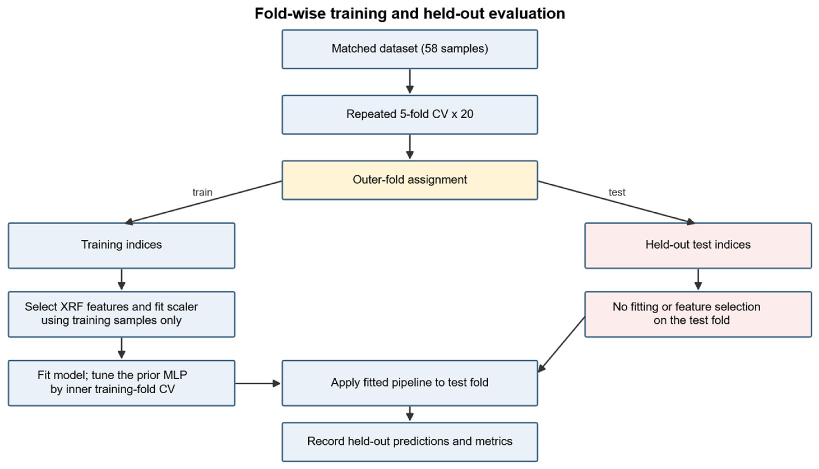
The modelling protocol was designed around a repeated outer cross-validation loop. Five-fold cross-validation was repeated 20 times with different random partitions, producing 100 held-out test folds. In each outer fold, all operations that could learn from the data—including XRF feature selection, feature scaling and hyperparameter tuning—were fitted using the training fold only. The held-out fold was reserved exclusively for prediction and metric calculation. Five-fold cross-validation was chosen over leave-one-out cross-validation (LOOCV) because LOOCV, while using more training samples per fold, produces highly correlated test predictions that can understate true prediction variance. Five-fold partitioning provides a better bias–variance trade-off for small datasets. The number of repetitions was set to 20 to ensure that the reported mean and standard deviation stabilize across different random partition sequences. A fixed random seed (42) was used for all experiments to ensure reproducibility. No stratification by TOC range was applied, because the continuous TOC distribution and small sample size make stratified binning unreliable; instead, the repeated random partitioning itself serves to distribute high- and low-TOC samples across folds over many repetitions.

This design prevents information from the held-out fold from entering XRF selection, scaling or model fitting. Hyperparameters of the prior MLP were selected by inner cross-validation using the outer training fold only. In this paper, the term strict cross-validation refers to this separation of training and testing operations; it does not imply that randomly partitioned samples are spatially independent. Spatial sensitivity was assessed separately with contiguous depth blocks and an exclusion buffer.

Figure 4 shows how each outer split is handled. The RepeatedKFold assignment sends training indices through feature selection, scaling and model fitting, whereas the test indices bypass all fitting steps. The trained pipeline is then applied once to the held-out samples to obtain predictions and metrics. The train and test branches are labelled directly in the revised figure.

3.2. Fold-Wise XRF Feature Selection

Within each outer training fold, the absolute Pearson correlation between each XRF element and TOC was calculated using training samples only [37]. The six highest-ranked elements were combined with AC, DEN, LR and GR. The six-element cap was fixed in advance to limit dimensionality because an outer training fold contains only 46 or 47 samples; it is not presented as a universal sample-to-predictor threshold. As a sensitivity check, mutual-information and LASSO-based selectors were also fitted within each outer training fold. With the same SVR and 100 outer partitions, Pearson selection gave RMSE = 0.789, compared with 0.839 for mutual information and 0.829 for LASSO (

Table A4. Feature-selection method comparison using 52 XRF elements under 100-fold cross-validation.

Method	RMSE Mean	RMSE SD	Fold-Wise Selection Summary
Pearson	0.7890	0.2667	Mo, V, Cr, Zn and Cd selected in all 100 folds
Mutual information	0.8389	0.2873	Most frequent: Ge (88), Nd (80), Be (78), Pr (69)
LASSO	0.8289	0.3046	Most frequent: Mo (96), Lu (75), Cd (74), V (69)
Logs only	1.2191	0.4048	Four log variables; no XRF selector

). Pearson selection was retained for the main analysis because it gave the lowest mean RMSE and the most stable selected set in this dataset. Elemental ratios were not screened because adding a large ratio library would require a larger dataset and nested control of the expanded search space.

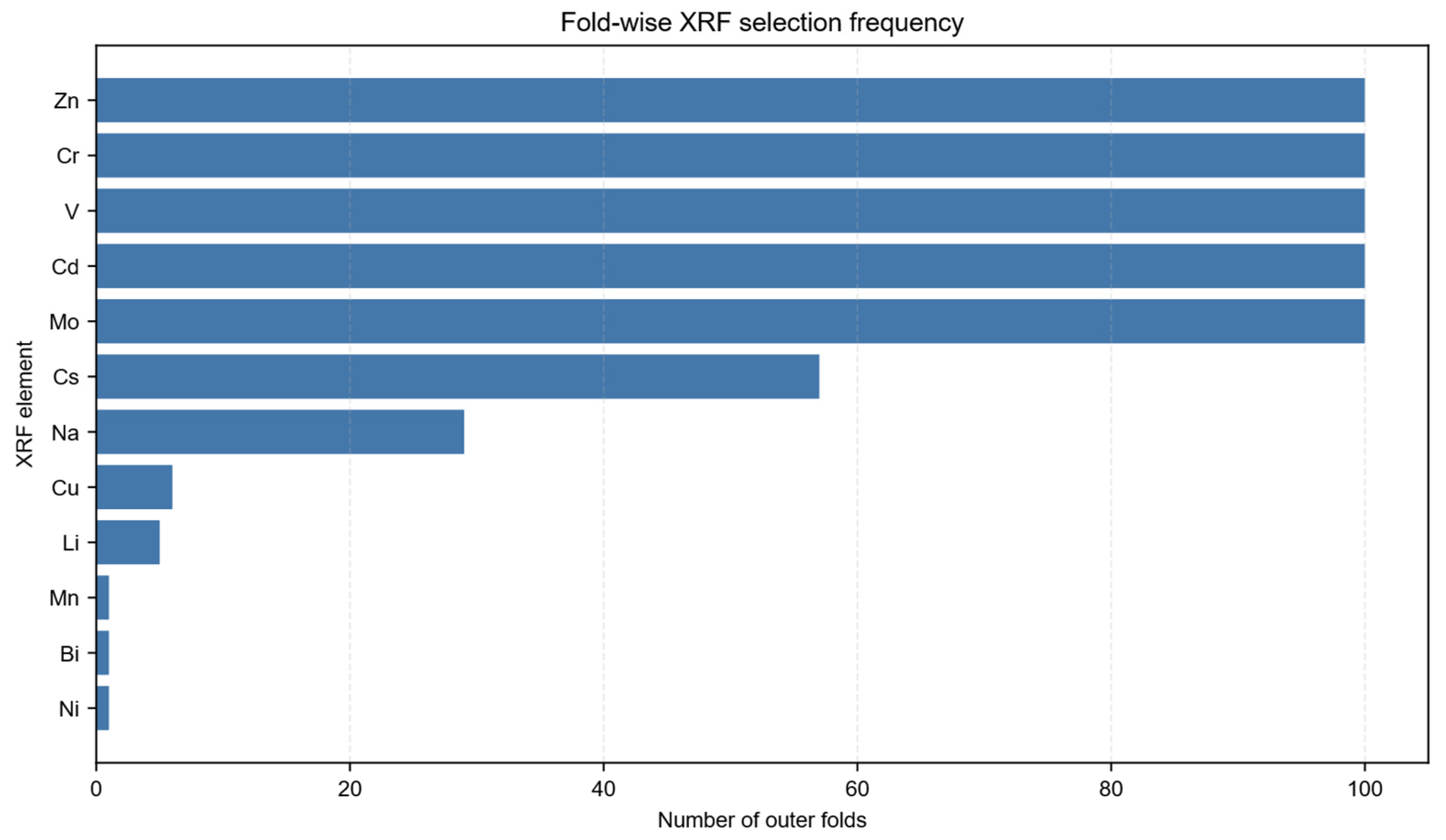
Selection frequency across the 100 outer folds was used as an indicator of stability.

Table 2. XRF feature-selection frequency across 100 outer folds.

Element	Selected Folds	Selection Frequency
Cd	100	100.0%
Cr	100	100.0%
Zn	100	100.0%
Mo	100	100.0%
V	100	100.0%
Cs	57	57.0%
Na	29	29.0%
Cu	6	6.0%
Li	5	5.0%
Bi	1	1.0%
Mn	1	1.0%
Ni	1	1.0%

reports the fold counts, and Figure 5 makes the distinction between consistently selected and occasional variables visible. An element selected in nearly every fold is less likely to be an artefact of one split, whereas an element selected only occasionally should be treated cautiously even if it appears in one fitted model. This frequency-based view is especially useful because the XRF variables are numerous and strongly correlated.

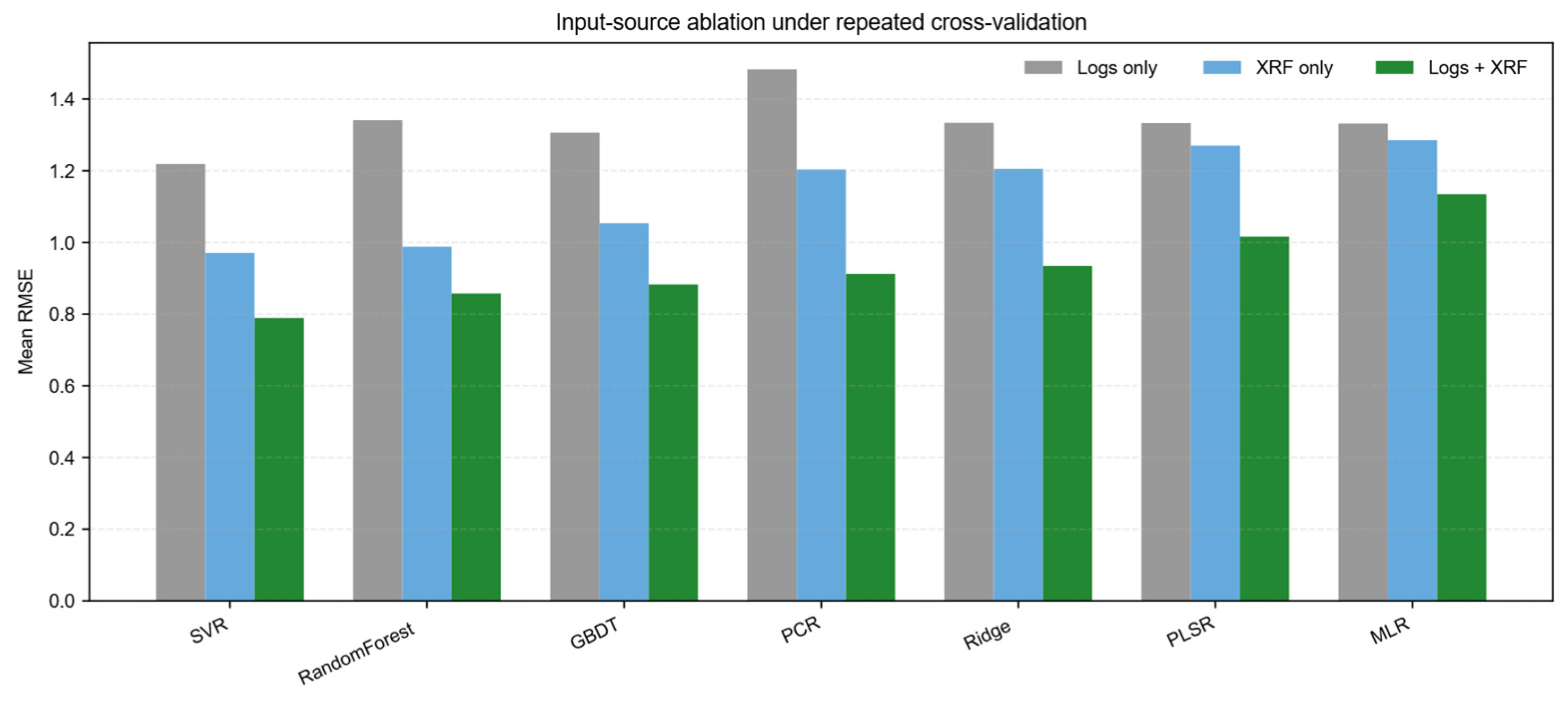
Three input settings were evaluated in the ablation analysis: logs only (AC, DEN, LR, GR), XRF only (six selected elements), and logs plus XRF (ten variables). The same outer folds were used for all three settings, so their fold-wise errors could be compared directly using paired statistical tests.

3.3. Model Settings

The candidate set organized in

Table 3. Candidate models and their role in the revised comparison.

Model Group	Models	Purpose in the Comparison	Validation Treatment
Linear baselines	MLR, Ridge	Check whether simple log–XRF relationships are sufficient	Fitted inside each outer training fold
Latent-variable baselines	PLSR, PCR	Reduce collinearity and dimensionality	Components selected without using held-out samples
Moderate nonlinear models	SVR, RandomForest, GBDT	Capture nonlinear response with controlled complexity	Parameters fixed or tuned inside training folds
Neural networks	BP-MLP, Optuna-prior MLP	Test whether optimized networks improve small-sample prediction	Inner validation only within training folds

spans interpretable linear baselines, moderate-complexity nonlinear models and neural-network variants. MLR was included as a conventional linear baseline and has precedent in petroleum-resource assessment [38]. Ridge regression, partial least-squares regression (PLSR) and principal-component regression (PCR) were used as regularized or dimension-reduced baselines [39,40,41]. Support vector regression (SVR), random forest (RF) and gradient boosting decision trees (GBDT) were used to test whether nonlinear relationships could be captured without the large number of trainable parameters required by deep networks [42,43,44].

Neural-network variants were retained as comparison models rather than treating them as presumptively superior. The BP-MLP used two hidden layers (8 and 4 units), tanh activation, the L-BFGS solver, alpha = 0.001 and a maximum of 3000 iterations [45]. The prior MLP used the same network after a power transform of the XRF inputs. Optuna with a TPE sampler [46] was run for three trials within each outer fold; a 3-fold inner cross-validation selected the XRF power (0.5–2.0) and alpha (10⁻⁴–10⁻¹, log scale).

Table A2. Hyperparameter search space, selection method and final values for each candidate model.

Model	Hyperparameters	Search Method	Search Space	Selected Value
MLR	None	None	None	None
Ridge	alpha	RidgeCV within outer training fold	13 values in logspace (−3,3)	Selected per fold
PLSR	n_components	Fixed	min(5, n_features-1)	5 fused; 3 logs only
PCR	PCA n_components	Fixed	min(5, n_features-1)	5 fused; 3 logs only
SVR	kernel, C, epsilon, gamma	Fixed	rbf, C = 10.0, epsilon = 0.1, gamma = scale	rbf, 10.0, 0.1, scale
RF	n_estimators, min_samples_leaf, max_depth	Fixed	500, 2, None	500, 2, None
GBDT	n_estimators, learning_rate, max_depth	Fixed	150, 0.05, 2	150, 0.05, 2
BP-MLP	layers, activation, solver, alpha, max_iter	Fixed	(8,4), tanh, lbfgs, 1 × 10−3, 3000	Same
Optuna-prior MLP	xrf_power, alpha	Optuna TPE; 3-fold inner CV; 3 trials	xrf_power: [0.5,2.0]; alpha: [1 × 10−4,1 × 10−1] log	Best per outer fold

reports the settings used in the reported runs.

Table A3. Comparison of similarities and differences among the nine candidate models.

Model	Type	Tunable Params	Dim. Reduction	Needs Scaling	Complexity	Strengths	Weaknesses
MLR	Linear	No	No	Yes	Low	Interpretable coefficients	Assumes linear relationships; sensitive to multicollinearity
Ridge	Linear + L2	Yes (alpha)	No	Yes	Low	Handles multicollinearity via L2 penalty	Still linear; alpha selected by CV
PLSR	Latent variable	Yes (n_comp)	Yes (PLS latent components)	Yes	Low	Handles correlated predictors; dimension reduction	Components may be hard to interpret geologically
PCR	PCA + linear	Yes (n_comp)	Yes (PCA)	Yes	Low	Dimension reduction before regression	PCA components not geochemically interpretable
SVR	Nonlinear (kernel)	Yes (C, gamma, eps)	No	Yes	Medium	RBF kernel captures nonlinear patterns; margin-based regularization	Kernel and hyperparameter choice affects results; not interpretable
RF	Tree ensemble	Yes (n_trees, depth)	No	No	Medium	Captures interactions; robust to outliers; feature importance	Can overfit with small data; less interpretable than linear
GBDT	Tree ensemble (boosting)	Yes (n_trees, lr, depth)	No	No	Medium	Sequential correction of errors; strong predictive power	Sensitive to learning rate; prone to overfitting if not tuned
BP-MLP	Neural network	Yes (layers, alpha, lr)	No	Yes	High	Universal approximator; flexible architecture	Sensitive to initialization; requires more data; black box
Optuna-prior MLP	Neural network (tuned)	Yes (xrf_power, alpha)	No	Yes	High	Automated hyperparameter optimization	Overfits inner validation on small data; computationally expensive

summarizes the key similarities and differences among the nine candidate models, including model type, complexity, dimensionality-reduction capability, scaling requirements, strengths and weaknesses.

All models were trained on the same outer-fold partitions. This ensures that differences in RMSE are caused by the modelling strategy and input setting rather than by different train–test splits. For models requiring standardized predictors, the scaler was fitted on the outer training subset and then applied to the corresponding held-out subset. For tree-based models, standardization was not expected to affect the splitting rules, but the same fold-wise data separation was maintained.

3.4. Metrics and Statistical Tests

Prediction performance was evaluated using mean absolute error (MAE), root mean square error (RMSE), Pearson correlation coefficient (R) and coefficient of determination (R²). Results are reported as mean ± standard deviation across the 100 outer folds. RMSE was used as the primary ranking metric because it penalizes large errors and is easy to interpret in TOC percentage units.

For the primary comparison, the five paired fold differences within each repeat were averaged, giving 20 repetition-level pairs for each model. Two-sided exact Wilcoxon signed-rank tests were applied to these 20 differences. Confidence intervals were obtained by bootstrapping the repetition-level differences 10,000 times, and Holm correction was applied across the seven conventional-model comparisons. The log-only versus fused SVR comparison was specified as confirmatory; the remaining models were used to assess whether the direction of the effect depended on model choice. Fold-wise standard deviations are retained as descriptive measures only. Because all repeats reuse the same 58 samples, these intervals describe stability to partitioning and do not replace external validation.

The permutation-importance calculation was also kept fold-aware. A predictor was permuted in the held-out subset after the model had already been trained on the corresponding training subset. The increase in held-out RMSE therefore measures how much the trained model depended on that predictor for unseen samples. This is more conservative than interpreting coefficients or importances from a model fitted once on the complete dataset.

Two additional sensitivity analyses were conducted. First, complete XRF sample rows were randomly reassigned to depths 500 times while the log–TOC pairs were retained. For each permutation, the full SVR pipeline, including training-fold XRF selection and scaling, was rerun. This preserves covariance among XRF elements while removing their alignment with the samples. Second, the depth-ordered data were divided into five contiguous test blocks. For each fold, training samples within 0.16 m of any test sample were excluded, with 0.16 m determined from the TOC autocorrelation analysis. The buffered result is reported as a five-fold sensitivity analysis rather than used for formal significance testing.

4. Results

This section reports the overall model comparison, the input-source ablation results, feature stability and variable importance, residual behaviour and the neural-network comparison.

4.1. Overall Model Comparison

Table 4. Model performance using fused log–XRF inputs under repeated cross-validation.

Rank	Model	MAE	RMSE	R	R2
1	SVR	0.550 ± 0.167	0.789 ± 0.267	0.912 ± 0.081	0.797 ± 0.178
2	RandomForest	0.614 ± 0.161	0.857 ± 0.241	0.900 ± 0.071	0.771 ± 0.157
3	GBDT	0.611 ± 0.156	0.883 ± 0.259	0.894 ± 0.070	0.761 ± 0.150
4	PCR	0.693 ± 0.191	0.912 ± 0.290	0.883 ± 0.088	0.736 ± 0.195
5	Ridge	0.710 ± 0.196	0.934 ± 0.298	0.877 ± 0.095	0.729 ± 0.195
6	PLSR	0.770 ± 0.200	1.016 ± 0.283	0.863 ± 0.099	0.679 ± 0.223
7	MLR	0.838 ± 0.224	1.134 ± 0.337	0.833 ± 0.132	0.588 ± 0.331
8	BP-MLP	0.908 ± 0.354	1.280 ± 0.544	0.779 ± 0.206	0.416 ± 0.582
9	Optuna-prior MLP	0.960 ± 0.362	1.329 ± 0.509	0.779 ± 0.189	0.389 ± 0.637

compares the nine candidate models on the same 100 fused-input outer folds.

Table 5. Input-source ablation under 100 outer folds; p-values are based on 20 repetition-level pairs.

Model	Logs Only	XRF Only	Logs + XRF	RMSE Reduction vs. Logs	Holm-Adjusted p
SVR	1.219	0.971	0.789	35.3%	1.34 × 10−5
RandomForest	1.341	0.988	0.857	36.1%	1.34 × 10−5
GBDT	1.306	1.052	0.883	32.4%	1.34 × 10−5
PCR	1.483	1.203	0.912	38.5%	1.34 × 10−5
PLSR	1.333	1.270	1.016	23.7%	1.34 × 10−5
Ridge	1.333	1.205	0.934	29.9%	1.34 × 10−5
MLR	1.332	1.285	1.134	14.8%	1.34 × 10−5

uses those same partitions and the same parameter settings to compare logs only, XRF only and fused inputs for seven conventional models. The two neural-network variants are retained in the overall ranking but are not included in the three-view ablation table.

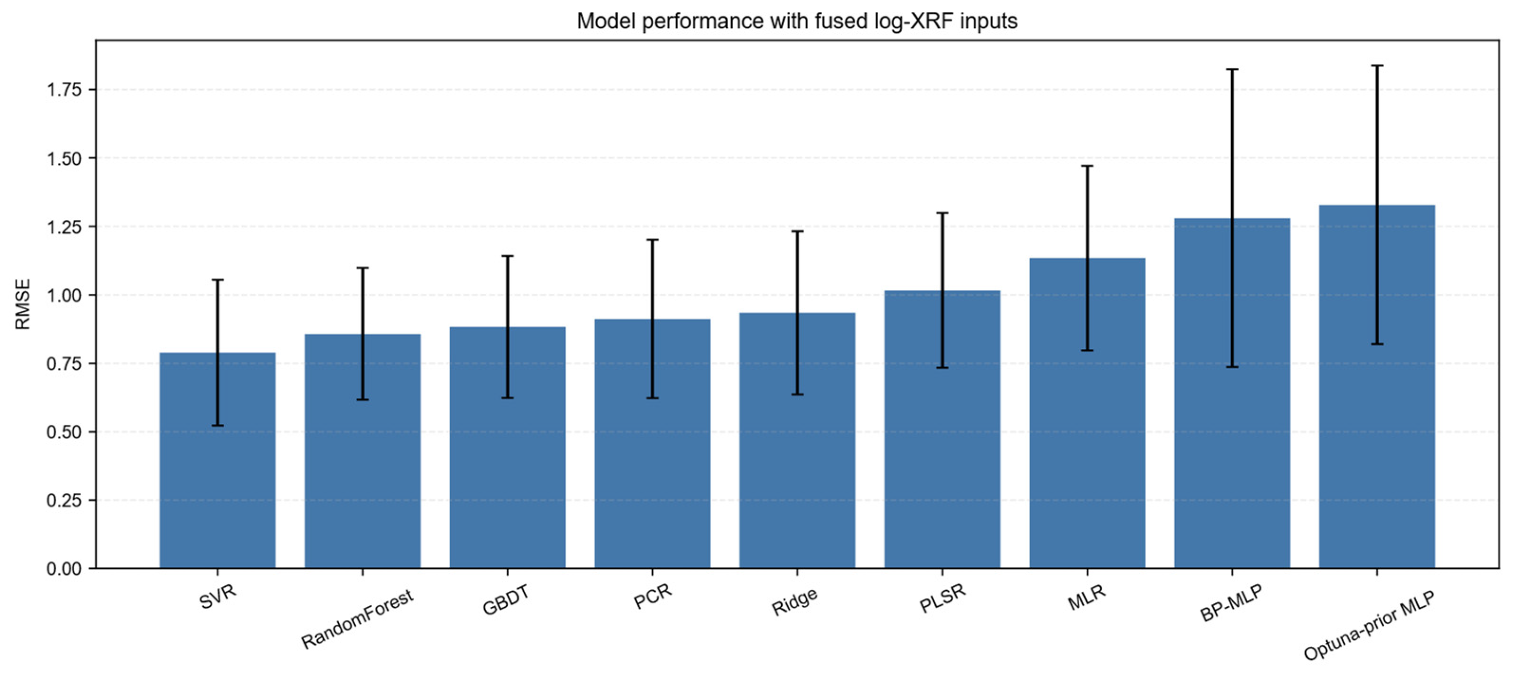
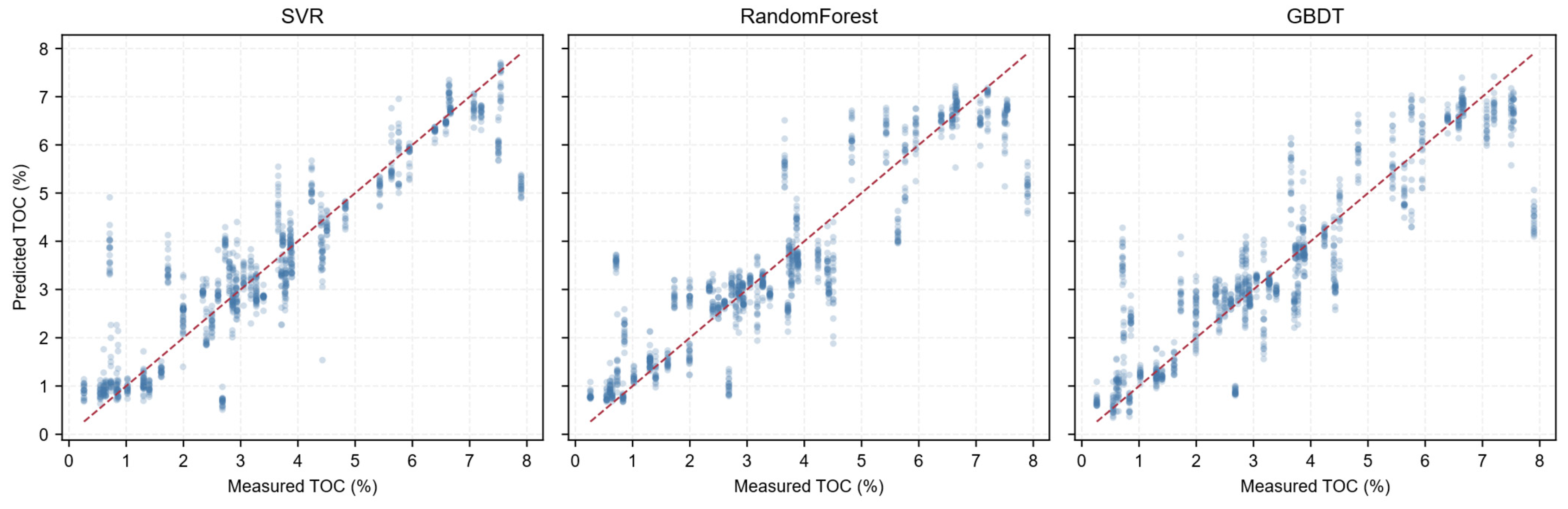
SVR ranked first among all tested models, with RMSE = 0.789 ± 0.267 and R = 0.912 ± 0.081. Random forest ranked second (RMSE = 0.857), followed by GBDT (RMSE = 0.883). Figure 6 shows the separation in mean RMSE, while Figure 7 shows the corresponding predicted-versus-measured relationships for the leading models. The three best models are nonlinear but do not rely on a large number of trainable neural-network weights, a pattern consistent with the small sample size and the correlated log–XRF predictor space.

Linear and latent-variable baselines performed reasonably but were consistently weaker than the leading nonlinear models. MLR produced the largest error among the traditional regression models, indicating that a simple linear combination of the selected variables cannot fully describe TOC variation in this interval. PCR and Ridge were more stable than MLR but did not match SVR, RF or GBDT.

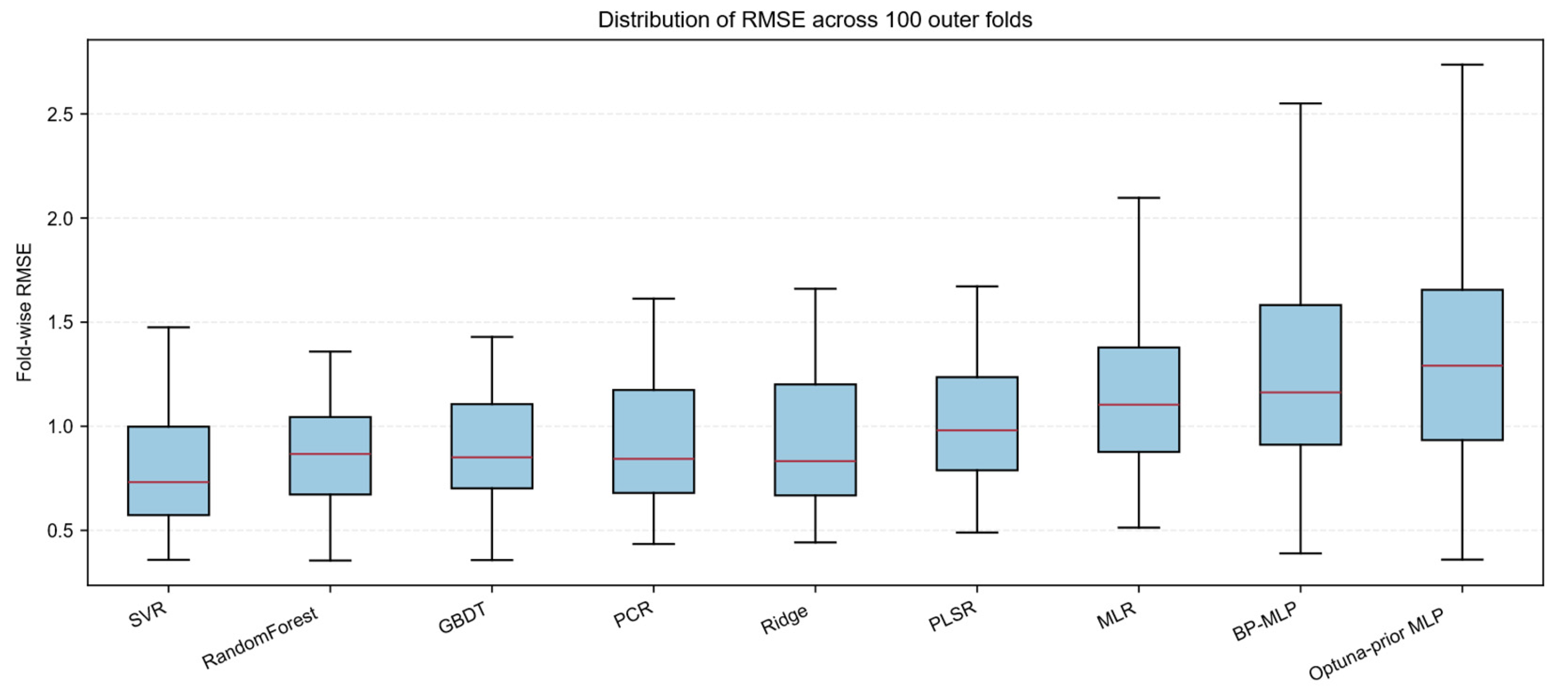
Figure 8 complements the mean RMSE ranking with the fold-wise error distributions. Models with similar mean RMSE values can still differ in robustness if one occasionally produces very large fold errors. SVR maintained a comparatively low error distribution across repeats, while the neural-network variants showed a wider spread. The leading model was therefore not only more accurate on average but also less dependent on a favourable validation split.

4.2. Contribution of XRF Data

To isolate the value of each data source, Table 5 compares log-only, XRF-only and fused inputs on the same 100 outer folds.

Table 5 summarizes the input-source comparison. XRF-only SVR (RMSE = 0.971) outperformed logs alone (RMSE = 1.219), while the fused input gave the lowest error (RMSE = 0.789). The corresponding uncertainty and sensitivity analyses are reported below. The corresponding model-wise comparison of log-only, XRF-only and fused inputs is shown in Figure 9.

For SVR, the mean RMSE decreased from 1.219 with logs alone to 0.789 with fused inputs. The repetition-level absolute reduction was 0.430 (95% CI: 0.386–0.478), corresponding to 35.3% (95% CI: 32.2–37.8%). All 20 repetition means favoured the fused input, although the fused RMSE was lower in 92 of the 100 individual folds; this distinction is why inference was performed at the repetition level. The exact two-sided Wilcoxon p-value was 1.91 × 10⁻⁶ and the Holm-adjusted value across seven models was 1.34 × 10⁻⁵. In the 500 XRF-row permutations, the mean null gain was −0.341 (SD = 0.108), and none reached the observed gain of 0.430 (empirical p = 0.002).

Table A1. Buffered contiguous depth-block validation (five folds; 0.16 m exclusion buffer).

Model	Logs-Only RMSE	XRF-Only RMSE	Fused RMSE	RMSE Reduction vs. Logs
SVR	2.5661	1.8274	1.8373	28.4%
RF	2.1899	1.9373	1.7512	20.0%
GBDT	2.5494	2.0343	1.6447	35.5%
PCR	2.0496	2.3085	1.9851	3.1%
Ridge	1.5706	2.0494	1.7481	−11.3%
PLSR	1.6164	2.4628	1.7882	−10.6%
MLR	1.4661	2.7523	2.1022	−43.4%

Note: In each fold, the naive-mean baseline predicted the test block using the mean TOC of the post-buffer training samples. Its mean RMSE was 2.132 ± 0.844 across the five blocks.

reports the contiguous depth-block sensitivity analysis with a 0.16 m exclusion buffer. The SVR fused RMSE was 1.837, compared with 2.566 for logs alone, a reduction of 28.4%. GBDT and random forest also retained clear reductions (35.5% and 20.0%, respectively), while PCR changed little. Ridge, PLSR and MLR did not benefit from fusion in this more conservative split. Thus, the added value of XRF remained evident for the main nonlinear models, but it was not universal across model classes when nearby training samples were excluded.

Under this design, the fused SVR RMSE of 1.837 corresponds to R² ≈ 0.22 relative to the TOC standard deviation of 2.076, while the logs-only SVR RMSE of 2.566 (R² ≈ −0.53) performed worse than a naive-mean baseline (RMSE = 2.132) computed in each fold using the mean TOC of the post-buffer training samples. Among all configurations in Table A1, MLR with logs alone achieved the lowest blocked RMSE (1.466, R² ≈ 0.50), suggesting that under severe spatial separation the simpler linear model may be more robust than the nonlinear SVR when only four log predictors are available. The five block-wise fused-SVR RMSE values were 1.754, 2.218, 2.524, 0.712 and 1.979, giving a mean ± SD of 1.837 ± 0.691 and a range of 0.712–2.524.

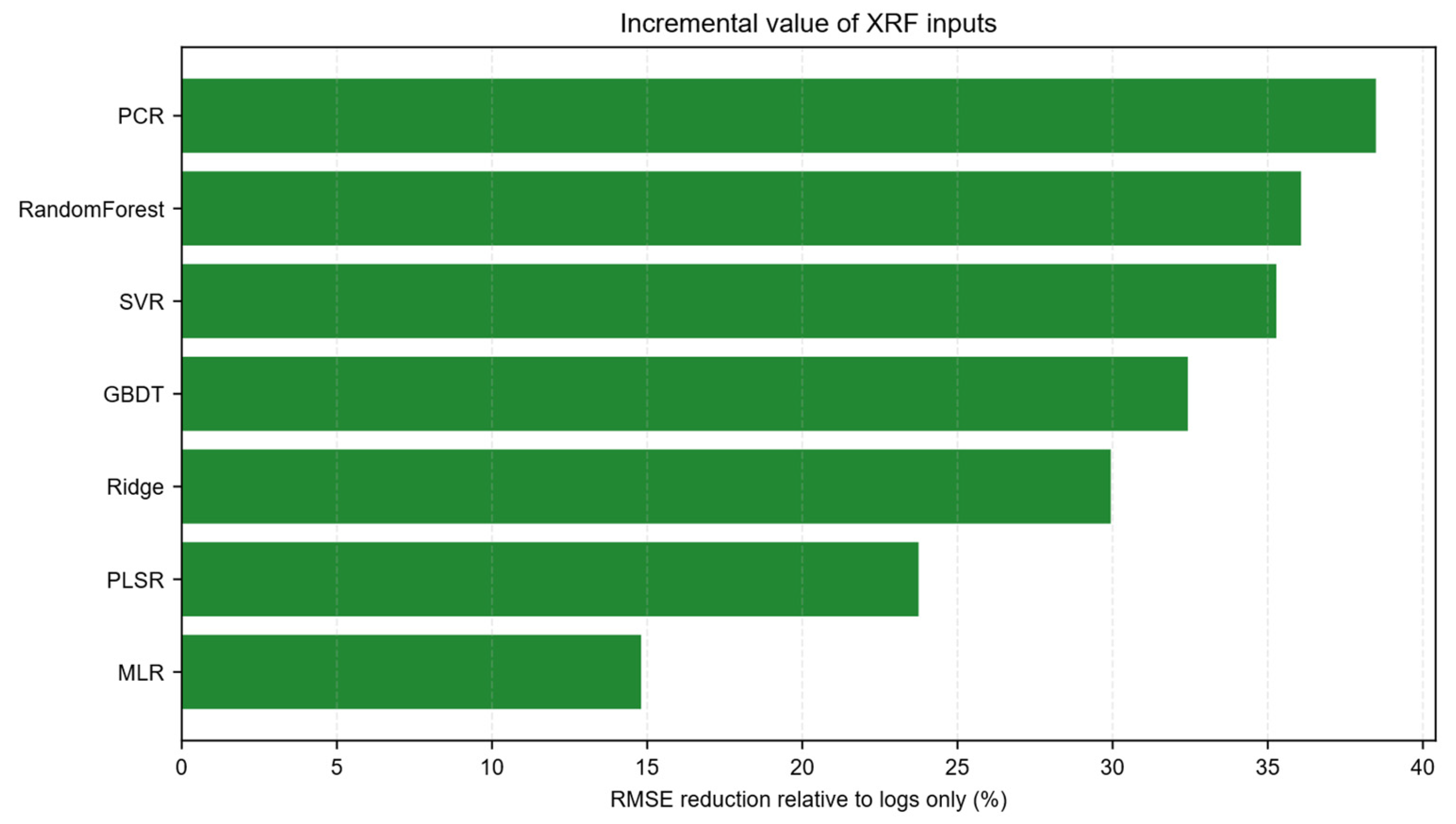
Figure 10 places the random-partition SVR result in the context of the other conventional models. Under the repeated random protocol, fused inputs reduced mean RMSE by 14.8–38.5% across the seven models, and all 20 repetition means were positive for each model. The corresponding Holm-adjusted p-value was 1.34 × 10⁻⁵. The buffered depth analysis gives a more qualified result, with the clearest gains confined to SVR and the tree-based models.

The ablation results also clarify the role of logs. XRF-only inputs performed well, but the best results were still obtained after adding the four log curves. This indicates that elemental composition is a strong TOC indicator in the sampled core interval, whereas continuous logging responses still provide useful physical constraints. In practical well evaluation, this is important because logs are available continuously, while XRF and TOC measurements are usually tied to discrete core or sampling positions.

4.3. Feature Stability and Variable Importance

Table 6. Stable SVR permutation importance estimated on held-out folds.

Feature	Selection Frequency	Mean RMSE Increase	SD
Mo	100.0%	0.554	0.292
AC	100.0%	0.411	0.176
Cr	100.0%	0.312	0.183
Cs	57.0%	0.271	0.176
V	100.0%	0.214	0.143
DEN	100.0%	0.203	0.163
LR	100.0%	0.199	0.157
Cd	100.0%	0.134	0.116
GR	100.0%	0.134	0.132
Zn	100.0%	0.117	0.099
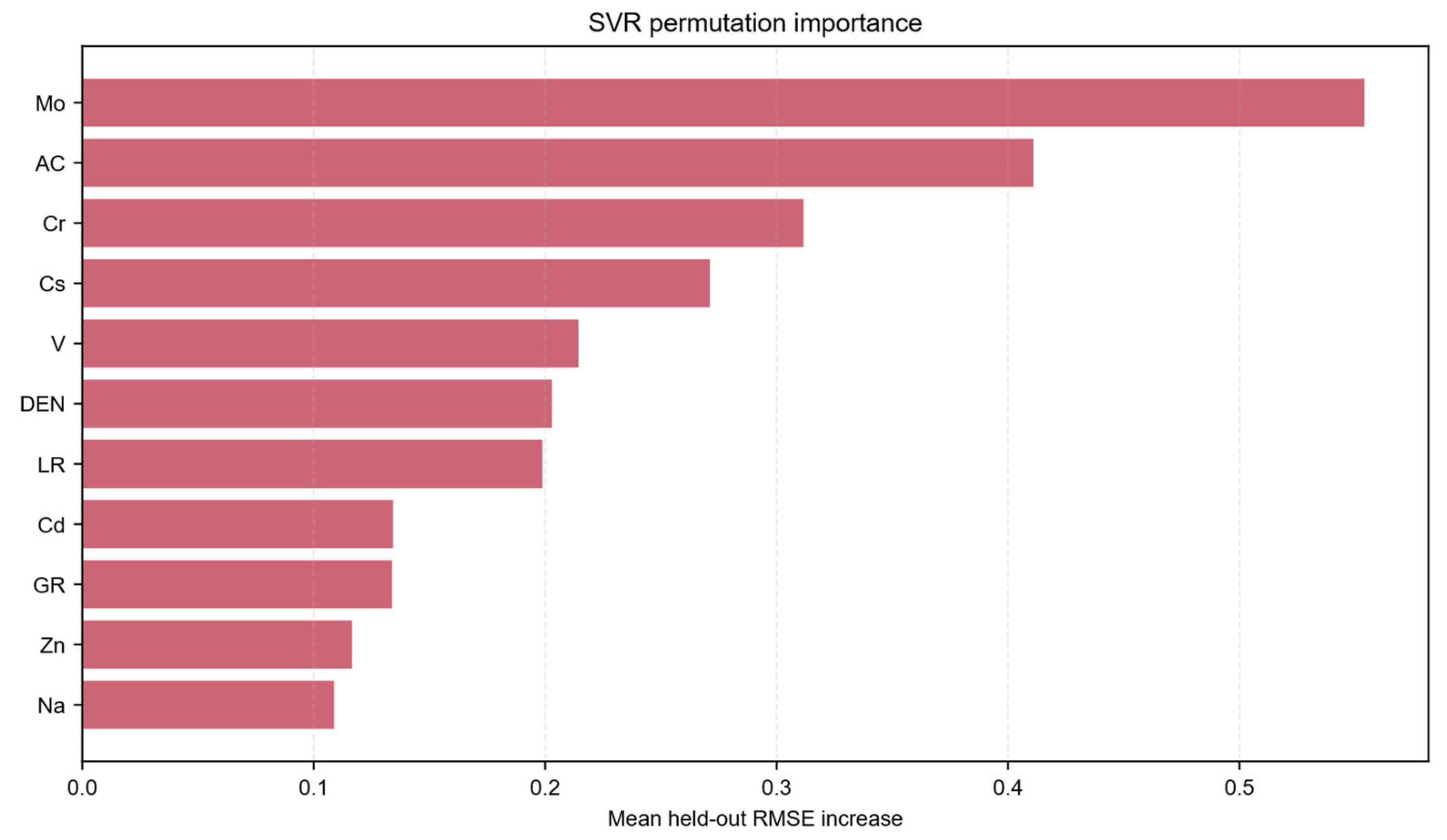
Na	29.0%	0.109	0.102

tests whether the variables selected most often were also important for held-out prediction by reporting fold-wise SVR permutation importance.

Cd, Cr, Zn, Mo and V were selected in all 100 Pearson-selection folds. Cs was selected in 57 folds, and several other elements were selected only occasionally. The frequent selection of Mo, V and Cr is consistent with their use as redox- or productivity-related indicators in organic-rich marine shale [24]. Cd and Zn may reflect organic matter or sulfide-associated enrichment, although this interpretation is not unique and should be checked against mineralogical evidence [24].

Mo produced the largest mean increase in held-out RMSE when permuted (0.554), followed by AC (0.411), Cr (0.312), Cs (0.271), V (0.214), DEN (0.203) and LR (0.199). Figure 11 makes the mixed composition of this ranking clear: geochemical variables and physical logs both contribute to the SVR predictions rather than one data source dominating the model.

The interpretation should remain cautious because the dataset is small and the elements are correlated. For example, a lower importance value for one element does not necessarily mean that the element is geologically irrelevant; it may share information with another selected element. Therefore, selection frequency, permutation importance and geological knowledge should be read together rather than treated as independent proof of causality.

4.4. Residual Behaviour and Depth-Profile Prediction

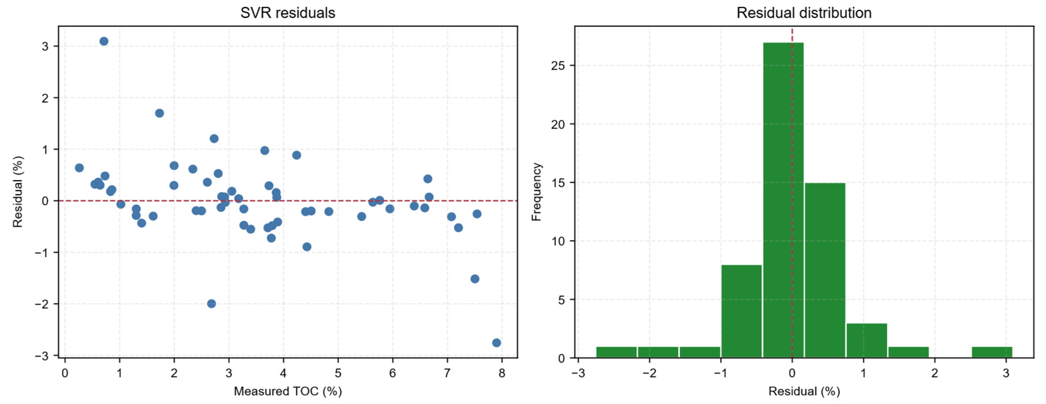
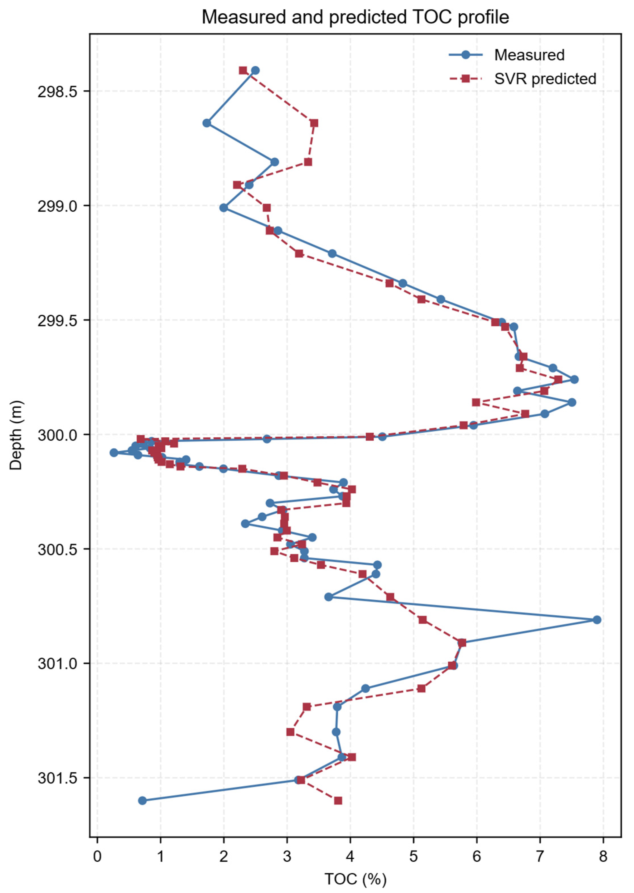
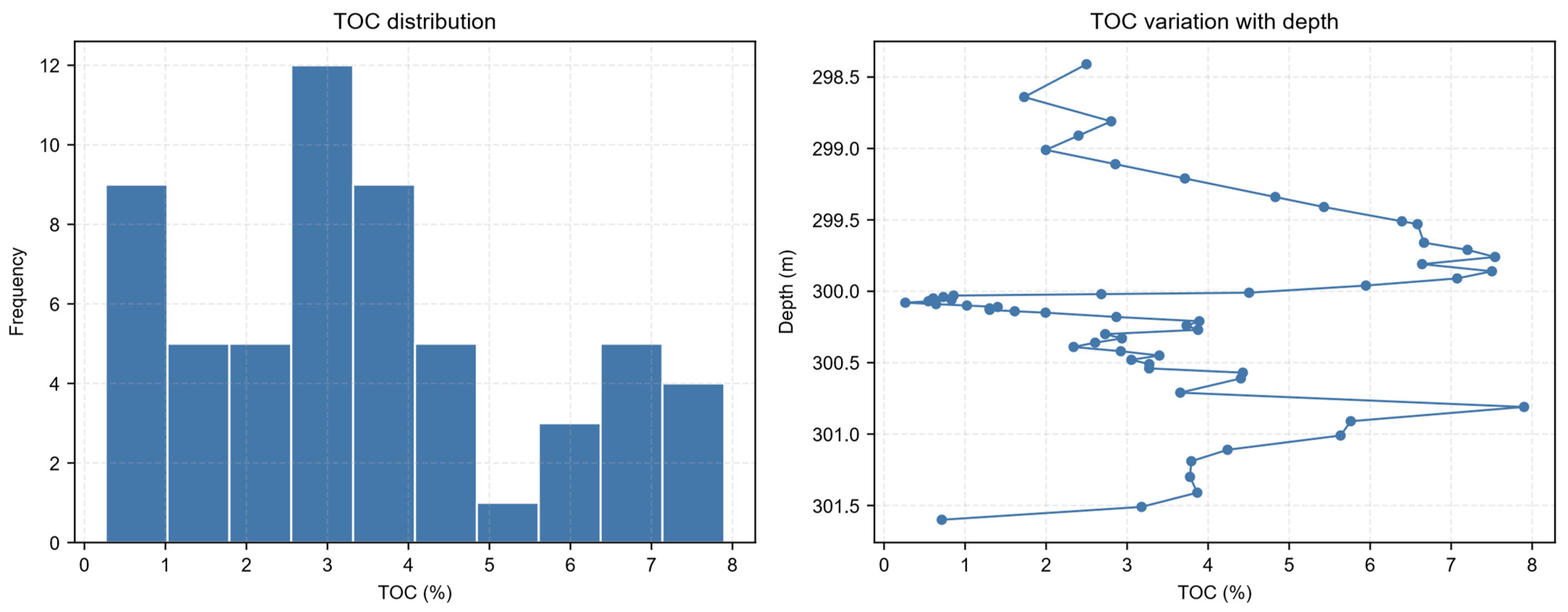
Averaged SVR predictions were aggregated at the sample level by collecting repeated held-out predictions for each depth. The residual distribution in Figure 12 is centred near zero, indicating that the model did not exhibit a strong systematic bias across the full TOC range. The largest absolute residual occurred at 301.60 m, where measured TOC was 0.712% and the averaged prediction was 3.807%, an error of 3.095 TOC percentage points. A second notable residual occurred at 300.81 m, where the maximum measured TOC of 7.900% was underestimated at 5.141% by 2.759 percentage points. Errors at these opposite extremes indicate that high-contrast local changes remain difficult to reproduce and that uncertainty increases near local maxima and minima.

Figure 13 compares measured and predicted TOC along depth. SVR captured the broad enrichment trend, including the main organic-rich interval between 299.34 and 299.96 m and the secondary enrichment around 300.57–300.61 m, but smoothed some sharp sample-to-sample fluctuations. Such smoothing is expected for a small dataset evaluated by repeated cross-validation and should be considered when the model is used for fine-scale stratigraphic interpretation.

The residual plot also suggests that prediction uncertainty increases near local extremes. This is a common limitation of data-driven regression when high values are represented by relatively few samples. For reservoir or source-rock evaluation, such uncertainty should be communicated explicitly, especially when the predicted TOC profile is used to identify high-quality intervals.

4.5. Neural-Network Variants

The neural-network comparison showed that a conventional BP network outperformed the Optuna-tuned prior MLP variant under the repeated cross-validation protocol (RMSE = 1.280 ± 0.544 vs. 1.329 ± 0.509). Neither neural-network variant provided a stable advantage over SVR (RMSE = 0.789) or the tree-based models (RF: 0.857; GBDT: 0.883). This does not imply that neural networks are unsuitable for TOC prediction in general; rather, it indicates that the present dataset is too small to support a strong claim that a more complex neural architecture is superior. Hyperparameter optimization can improve a neural network when sufficient validation data are available, but it can also overfit the inner validation signal in small datasets. In the present case, the simpler SVR baseline is more defensible than a neural-network model with a larger search space.

5. Discussion

This section interprets the value of log–XRF fusion, explains why moderate-complexity models performed best, compares the present results with previous studies, and discusses limitations and transferability.

5.1. Value of Log–XRF Fusion

We now return to the three questions raised in Section 1. First, under repeated random cross-validation, fused inputs produced lower mean RMSE than logs alone for all seven conventional models; reductions ranged from 14.8% for MLR to 38.5% for PCR, with a 35.3% reduction for SVR. Second, the SVR gain was positive in all 20 repetition means; under buffered contiguous depth validation, RMSE decreased from 2.566 to 1.837 (28.4%), although the buffered result was not shared by every linear model. Third, Mo, V, Cr, Cd and Zn were selected in all 100 Pearson folds and had positive mean held-out permutation importance. Together, these results support an incremental XRF contribution within this well without implying that the magnitude is independent of validation design.

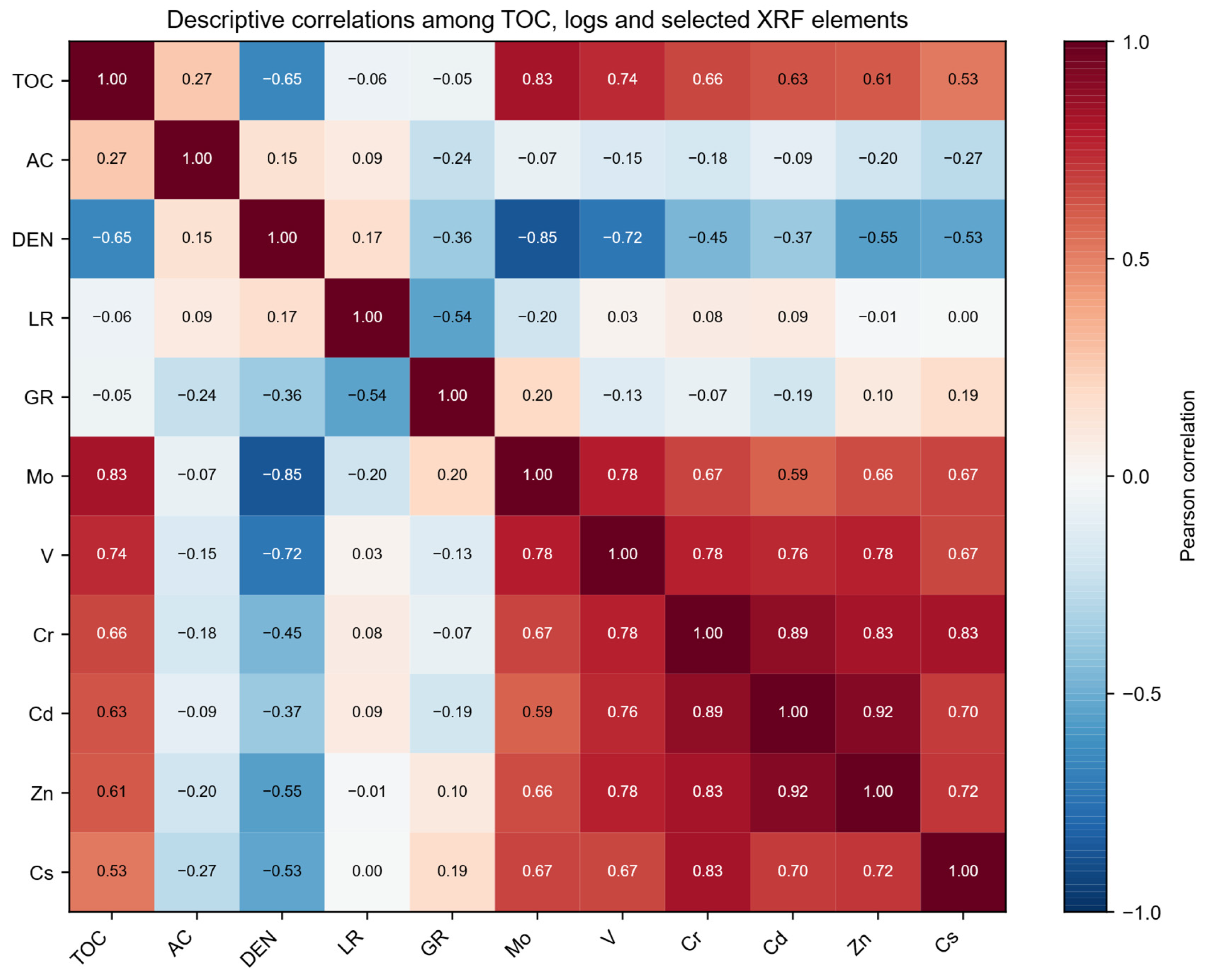
The correlation and importance analyses provide a geological context for the predictive results. DEN is negatively correlated with TOC (r = −0.65), consistent with the lower density commonly associated with organic-rich shale. AC reflects changes in rock fabric and elastic properties. Mo, V, Cr, Cd and Zn were repeatedly selected, but they are not direct measurements of organic carbon. Trace-metal proxies may record depositional redox, productivity, sulfide formation and later diagenetic modification [24]; consequently, their predictive importance should not be read as a unique process attribution.

5.2. Why Moderate-Complexity Models Performed Best

The superiority of SVR, RF and GBDT over neural-network variants is reasonable for a dataset with only 58 labelled samples. SVR with a radial basis function kernel [42] can model nonlinear relationships while controlling complexity through margin-based regularization. Tree ensembles [43,44] can capture threshold and interaction effects without requiring gradient-based training of many weights. In the present study, the BP-MLP and Optuna-prior MLP yielded the two highest cross-validated RMSE values among the candidate models (Table 4), indicating that their additional architectural complexity did not improve prediction for this 58-sample dataset.

This finding suggests that the main methodological value lies in rigorous small-sample data fusion rather than in architectural complexity. A clear validation protocol, transparent ablation and interpretable feature analysis are more defensible than a complicated neural-network architecture when independent external validation is not available. The result also provides a useful reminder that model selection should be controlled by validation evidence rather than by the apparent sophistication of the algorithm.

5.3. Comparison with Previous Studies

Regarding robustness, averaging the five folds within each repeat gave 20 paired repetition-level comparisons, all of which favoured fused SVR. At the individual-fold level, 92 of 100 comparisons favoured fusion. Regarding feature stability, Mo, V, Cr, Cd and Zn were selected in every Pearson fold and had positive mean held-out permutation importance. Several previous studies have integrated well logs with geochemical data for TOC prediction or source-rock characterization [27,28,29,32]. Chan et al. [32] is the closest comparison: they combined XRF elements with conventional logs in an ANN and reported improved accuracy over empirical methods. The present study differs by using matched input-source ablation, repeated leakage-controlled partitions and a separate depth-buffered sensitivity analysis.

Wang et al. [16] addressed the small-sample problem through unsupervised contrastive learning, which is a complementary approach. Their method leverages unlabeled data for pretraining, whereas the present study focuses on strict validation protocol and data-source ablation. Both strategies acknowledge that small datasets require special care, but they operate at different levels: representation learning from unlabeled logs versus evaluation rigour and input-source attribution.

Khan et al. [30] applied a stacking model with SHAP-based feature importance for Longmaxi shale TOC prediction. Their study used a larger three-well dataset and reported high accuracy (R² = 0.964). It included both an 80/20 holdout split and leave-one-well-out validation, but did not report repeated resampling or input-source ablation. Li et al. [31] first used SOM clustering to distinguish lithologic groups, and then applied PSO-optimized SVM-RFE to select logging variables and constructed separate SVR models for the resulting groups, achieving a mean relative error of approximately 6%. Their feature-selection approach (SVM-RFE) is more sophisticated than the correlation-based method used here, but it was also not evaluated across repeated folds. Zhao et al. [23] applied feature engineering (log transformation and polynomial features) with XGBoost to predict TOC from conventional logs in the Dongying Depression, Bohai Bay Basin. Their study achieved good prediction accuracy but used well logs alone without XRF data, employed a single train–test split, and focused on feature construction rather than input-source ablation. The present study differs in three respects: (1) we integrate XRF elemental data with logs and quantify the incremental value through ablation; (2) we employ repeated 100-fold cross-validation with fold-wise preprocessing; and (3) we evaluate feature stability across 100 folds rather than relying on a single model fit.

5.4. Implications for TOC Prediction in Limited-Data Wells

Many wells in shale exploration have limited core TOC measurements but may have continuous logs and additional geochemical scanning data. The workflow used here is therefore practical: it does not require a large training set, and it can be repeated for other wells by replacing the input data while keeping the same fold-wise preprocessing logic. The model can be used to screen intervals with relatively high organic matter potential, but its predictions should be interpreted together with geological knowledge rather than as a replacement for laboratory geochemistry.

The residual and depth-profile analyses also show where caution is needed. The model captures the broad vertical pattern but smooths some local extremes. If the purpose is high-resolution stratigraphic correlation or sweet-spot boundary delineation, additional samples near abrupt TOC changes would be valuable. Without such samples, the model is better suited for interval-scale prediction than for interpreting every small fluctuation.

5.5. Limitations

The main limitation is the absence of an independent well or additional core interval. Repeated cross-validation describes internal stability better than a single split but cannot establish regional generalization. Spatial dependence is also substantial: the lag-1 TOC autocorrelation is 0.883, and the estimated correlation length is approximately 0.16 m. The buffered depth analysis produced higher absolute errors and showed that the fusion gain was model-dependent. The term strict in this study therefore refers to prevention of preprocessing leakage, not to proof of spatial independence.

The buffered analysis also showed that MLR with logs alone achieved the lowest blocked RMSE (1.466), outperforming all fused configurations, and that the logs-only SVR performed worse than a naive-mean baseline. These results indicate that the fusion benefit is not universal under spatial separation and should be interpreted with caution.

A second limitation concerns feature selection. Pearson ranking performed better than the mutual-information and LASSO alternatives tested here, but all three methods may vary in another well or formation. Pearson ranking also does not resolve multicollinearity or test geochemical ratios. Future work should evaluate a prespecified set of ratios and mineralogical proxies within nested validation, preferably using more wells. The permutation test shows that the XRF block contains predictive information, but it does not establish a unique causal interpretation for individual elements.

5.6. Transferability and Future Work

The workflow is transferable in the sense that it defines where each data-processing step should occur inside the validation loop. However, the selected elements and the fitted model should not be transferred mechanically to another well without revalidation. Different shale intervals may have different mineral assemblages, redox histories, maturity levels and logging responses. Applying the workflow to another well should therefore involve new fold-wise feature selection and, ideally, an independent external test.

Future work should focus on three directions. First, additional wells or additional core samples are needed to test external generalization. Second, geologically meaningful XRF ratios and mineralogical proxies should be evaluated under the same framework. Third, uncertainty estimates should be reported together with predicted TOC profiles so that high-TOC intervals can be interpreted with appropriate confidence.

6. Conclusions

A log–XRF fusion strategy for TOC prediction was evaluated using 58 matched samples from the Yiwan-1 well, with feature selection, scaling and model fitting confined to training folds of repeated cross-validation.

Using fused well-log and XRF inputs, SVR achieved the best overall performance among the tested models, with RMSE = 0.789 and R = 0.912. Random forest and GBDT also performed well, whereas complex neural-network variants did not show a stable advantage in this small-sample setting.

Input-source ablation showed an incremental contribution from XRF data within the Yiwan-1 dataset. For SVR, mean RMSE decreased by 35.3% under repeated random cross-validation; the repetition-level reduction was 0.430 (95% CI: 0.386–0.478; Holm-adjusted p = 1.34 × 10⁻⁵). Under buffered contiguous depth validation, RMSE decreased from 2.566 to 1.837 (28.4%), although the buffered result was not consistent across all linear models.

Mo, Cr, V, Cd and Zn were selected in all 100 Pearson-selection folds, while Cs was selected in 57. Their positive mean held-out permutation importance indicates predictive relevance in this dataset, but geological interpretation requires independent mineralogical and multi-well evidence.

Because no independent validation well is available, these results demonstrate internal predictive consistency rather than regional generalization. The fusion strategy itself—separating data-source contributions, quantifying XRF incremental value, and identifying stable geochemical indicators—is transferable to other wells where limited core measurements are supplemented by geochemical scanning.