Frequency-Domain Enhancement and Multi-Scale Residual Modeling for Single-Image Reflection Separation

Abstract

Single-image reflection separation aims to recover transmission and reflection layers from an image captured through glass and is an important problem in computational photography and low-level vision. Recent dual-stream interactive methods have achieved substantial progress, but most of them still rely mainly on linear spatial-domain feature modeling and single-scale residual prediction, which limits their ability to handle complex reflection mixtures. To address these issues, this paper proposes a structural enhancement method for a pretrained dual-stream baseline. Inspired by homomorphic filtering, a Homomorphic Frequency Enhancement Module (HFEM) extracts complementary frequency-domain features through a logarithmic transformation and Haar wavelet decomposition and injects them into the local-prior branches of both streams via zero-initialized projections. A multi-scale residual modeling module (MSRM) further aggregates multi-level decoder features to replace the original single-scale residual module. During training, the pretrained baseline is kept frozen, and only the newly introduced modules are optimized. The final implementation introduces 1.528 M additional trainable parameters, including 1.318 M from HFEM and 0.210 M from MSRM, accounting for approximately 0.47% of the complete 328.49 M-parameter adapted model. On five public benchmarks with 494 images in total, the proposed method improves the weighted-average PSNR/SSIM from 26.52 dB/0.916 to 26.74 dB/0.917. Although the overall gain is modest, the frozen training setting shows a more stable optimization process, with a PSNR fluctuation of 0.28 dB compared with 3.65 dB for joint fine-tuning. Ablation results indicate that HFEM is the primary source of the performance gain, while MSRM provides a complementary residual-modeling benefit.

1. Introduction

When a camera captures an image through a semi-reflective medium such as glass, a shop window, or a vehicle window, the signal received by the sensor usually consists of two components: transmitted light from the target scene behind the glass and reflected light from the environment in front of the glass. These components overlap on the imaging plane and form a mixed image containing reflection artifacts. This degradation is widespread in shop-window photography, onboard vision, surveillance, and other real-world scenarios. It not only reduces visual quality but can also damage object boundaries, texture details, and semantic structures, thereby affecting the reliability of downstream tasks such as object detection, semantic segmentation, and three-dimensional reconstruction. Single-image reflection separation (SIRS) aims to recover both the transmission and reflection layers from only one mixed image and is a fundamental yet challenging problem in computational photography and low-level vision [1,2]. Recent research on dual-channel blind image separation further treats reflection and shadow layer separation as representative mixed-image recovery problems and explores wavelet-domain interaction for separating coupled sources [3].

From a signal-processing perspective, SIRS is a highly underdetermined blind source separation problem. Given an observed image, the imaging process is commonly modeled as the sum of a transmission layer, a reflection layer, and a residual term describing nonlinear effects [4], i.e., $I=T+R+\mathsf{\Phi }(T,R)$. A single image must constrain two unknown image layers and a possible nonlinear residual, so the decomposition satisfying this imaging constraint is not unique. Traditional methods narrow the solution space with handcrafted statistical or physical priors, such as relative smoothness [5] and ghosting cues [6]; deep-learning methods instead learn data-driven reflection-separation priors from training data. Nevertheless, real reflections vary substantially in intensity, sharpness, spatial distribution, and their degree of entanglement with the transmission layer, leaving SIRS incompletely solved.

Deep SIRS methods have broadly progressed from single-stream restoration to dual-stream reconstruction and then dual-stream interaction. Early single-stream methods [7,8] generally treated reflection as a degradation to be suppressed and focused on recovering the transmission layer. Later dual-stream methods [9,10] estimated both layers and used their complementary constraints to facilitate separation. More recent dual-stream interactive methods [4,11,12] introduced explicit feature exchange, attention-based interaction, or inter-layer association modeling to strengthen information flow between the two representations. Across this progression, most improvements have concentrated on how the transmission and reflection features interact, whereas the underlying assumption of how the two layers are superimposed during imaging has received less attention. In other words, despite architectural advances, most methods implicitly retain a linear additive formation model whose applicability to real glass-reflection scenes has not been fully examined. This observation motivates us to reconsider existing SIRS frameworks from the perspectives of reflection superposition and residual modeling.

Issue 1: Lack of a logarithmic-domain frequency prior. Existing SIRS methods usually describe reflection superposition with a linear additive model. Real imaging through glass, however, is often affected by spatially varying transmittance and can be expressed by the weighted mixture

$$I(x,y)=T(x,y)\alpha (x,y)+R(x,y)\left[1-\alpha (x,y)\right].$$

(1)

where $\alpha (x,y)$ is the spatially varying transmittance determined by factors such as glass material, incident angle, and local illumination [13]. Unlike a simple linear additive model, Equation (1) multiplicatively couples the transmission layer with the transmittance field, while the reflection layer is also spatially modulated by that field. Conventional spatial-domain feature extraction alone, therefore, has difficulty explicitly describing this modulation.

Homomorphic analysis provides a classical way to address multiplicative coupling [14,15]: taking the logarithm of a product converts multiplication into addition. Inspired by this principle, we explore frequency decomposition of an input image in the logarithmic domain, providing the network with a complementary path distinct from linear spatial-domain features. Because Equation (1) remains a sum of two modulated components, the logarithmic transformation cannot analytically decompose the reflection mixture. We, therefore, do not claim that the logarithmic domain precisely separates reflection; instead, we use it as a complementary feature source with statistical characteristics different from those of the conventional spatial domain.

Issue 2: Insufficient single-scale modeling of nonlinear residuals. In addition to the linear additive terms, real reflection formation may contain nonlinear factors such as multiple reflections, overexposure and saturation, energy attenuation, and local transmittance variation. These factors are commonly grouped into a residual term [4]. Although existing dual-stream frameworks explicitly model this term as a learnable component, their residual prediction generally relies on local features at a single decoder scale. Shallow, single-scale features lack guidance from high-level semantics and global structure, even though the spatial distribution of residuals is often closely related to scene content. A single-resolution representation is also unable to describe large-scale smooth attenuation and small-scale local distortion simultaneously. Thus, even if more discriminative frequency features are introduced at the encoder, a single-scale residual branch may fail to use them fully. We therefore introduce multi-scale residual modeling to improve cross-scale contextual awareness. Research on general image restoration likewise shows that multi-resolution feature fusion, multi-stage interaction, and hierarchical encoder–decoder structures help balance local detail and contextual information [16,17,18].

The main contributions are summarized as follows:

• We propose a Homomorphic Frequency Enhancement Module (HFEM), which introduces frequency-domain information complementary to the spatial domain through a logarithmic transformation and Haar wavelet decomposition, and injects it into the local-prior branches of both streams via zero-initialized projections. HFEM is the main architectural contribution and the primary source of the performance gain reported in this work.
• As a complementary residual-modeling component, we introduce a multi-scale residual modeling module (MSRM) that aggregates multi-level decoder features to replace the original single-scale residual module. The ablation results show that MSRM alone provides a limited gain, improving Average494 PSNR by about 0.08 dB, while adding MSRM on top of HFEM brings a further modest improvement of 0.03 dB. Therefore, MSRM is positioned as a supporting design rather than an equally dominant independent contribution.
• At the training-strategy level, we keep the pretrained baseline frozen and optimize only the newly introduced HFEM and MSRM. The final implementation introduces 1.528 M trainable parameters, including 1.318 M from HFEM and 0.210 M from MSRM, accounting for approximately 0.47% of the complete 328.49 M-parameter adapted model. This frozen-baseline setting improves the interpretability of ablation analysis and yields a more stable optimization process, with a PSNR fluctuation of 0.28 dB compared with 3.65 dB for joint fine-tuning. It is described as a training strategy for stable adaptation rather than an independent architectural contribution.

2. Related Work

2.1. Single-Image Reflection Separation

Early SIRS studies mainly relied on handcrafted statistical or physical priors that exploited differences between transmission and reflection layers in smoothness, gradient distributions, and imaging geometry. Li and Brown [5] separated layers using their relative smoothness; Shih et al. [6] used ghosting cues produced by double-pane glass to assist reflection recovery; Arvanitopoulos et al. [19] combined a Laplacian data term with a sparse gradient prior for reflection suppression; and Levin and Weiss [20] guided separation with user annotations and a sparsity prior. Such methods can be effective when their imaging assumptions hold, but their performance depends strongly on how well a fixed prior matches the actual scene. The wide variation in real reflections limits their generalization.

With the development of deep learning, data-driven approaches gradually became the mainstream for SIRS [21]. Early deep methods mostly adopted a single-stream restoration framework that directly predicted a clean transmission layer. CEILNet [22] divided reflection removal into edge-map estimation and image restoration, using edge information to guide transmission reconstruction. Zhang et al. [23] introduced perceptual and exclusion losses that exploited gradient-domain differences between the layers. ERRNet [7] further developed a network that can learn from misaligned image pairs, alleviating the difficulty of obtaining precisely aligned real training data. These approaches advanced transmission restoration but did not explicitly recover and use the reflection layer. Because the two layers provide complementary constraints, ignoring structural cues in the reflection layer can restrict modeling of their mixture and motivated subsequent dual-stream methods.

Dual-stream methods began to restore both transmission and reflection and to constrain separation through their complementary relationship. IBCLN [9] used a cascaded refinement strategy based on long short-term memory networks to iteratively update the two predictions. Yang et al. [10] proposed a bidirectional estimation network in which the two branches guide each other. Compared with single-stream methods, these frameworks explicitly retain reflection representations and provide a basis for modeling inter-layer dependencies.

Researchers subsequently introduced explicit dual-stream interaction mechanisms. YTMT [12] uses rectified linear units and negative rectified linear units to pass information suppressed in one branch to the other. DSRNet [4] designs a MuGI interaction module and introduces a learnable residual term to unify different reflection-formation models. DSIT [11] further uses dual-stream self-attention and layer-aware dual-stream cross-attention to model intra- and inter-layer correlations explicitly, while incorporating a frozen pretrained Transformer for semantic priors [24,25]. Because DSIT is representative in its dual-stream interaction and use of pretrained features, we adopt it as the baseline.

DSIT is adopted as the baseline because it is representative of recent dual-stream interactive SIRS frameworks: it combines a pretrained Transformer prior, local dual-stream priors, and an interaction decoder for joint transmission–reflection modeling. However, its feature representation is still mainly constructed in the spatial domain, and its residual prediction relies on a single decoder scale. These design choices may limit its ability to represent spatially varying transmittance and cross-scale nonlinear residuals. Therefore, instead of redesigning the entire backbone, this work studies whether complementary logarithmic-domain frequency features and multi-scale residual modeling can enhance a frozen pretrained dual-stream baseline. This setting also makes the contribution of the newly introduced modules easier to analyze.

Recent studies have also advanced SIRS through robustness, data construction, pretrained-model adaptation, and user interaction. RobustSIRR [26] examines robustness against adversarial perturbations. GFRRN [27] adapts a pretrained model to reduce semantic gaps with reflection removal and uses unified labels to reduce label inconsistency between synthetic and real data. RDNet [28] uses reversible decoupling to improve layer separation. RRW [8] designs a cascaded detection–removal strategy and a more efficient data-acquisition process. DURRNet [29] and DExNet [30] explore deep unfolding networks, while FIRM [31] supports interactive removal. Recent work also targets realistic RAW-photo processing [32], and the NTIRE 2025 challenge establishes an in-the-wild benchmark for evaluating practical reflection-removal systems [33]. Unlike these works, we retain the dual-stream interaction mechanism and structurally enhance it through two relatively orthogonal directions: logarithmic-domain frequency modeling and multi-scale residual modeling.

Very recent CVPR 2026 studies continue to advance SIRS from complementary directions, including parameter-efficient adaptation of pretrained models with adaptive frequency learning [27], lightweight network design [34], generative latent-space rectification [35], and polarization-based reflection removal [36]. Our method is complementary to these efforts: it injects logarithmic-domain frequency features and multi-scale residual modeling into a frozen dual-stream baseline.

2.2. Frequency-Domain Methods in Image Restoration

Frequency analysis is an important signal-modeling tool in image restoration. Instead of processing pixels only in the spatial domain, transforms decompose an image into frequency components so that low-frequency structure and high-frequency texture can be modeled separately. Wavelet transforms, Fourier transforms, and adaptive frequency modulation have been widely used for denoising, super-resolution, and general restoration [37,38,39]. Multi-level wavelet convolutional networks [40,41] process frequency subbands at different scales to improve detail reconstruction. AdaIR [42] further introduces adaptive frequency mining and modulation to adjust frequency responses according to degradation type. For SIRS specifically, WDUNet combines discrete wavelet decomposition with deep unfolding to model reflection information in frequency subbands [43]. Frequency information has also been used in reconstruction losses [44], image deblurring networks [45], and interactive frequency–spatial restoration frameworks [46]. These findings demonstrate that explicit frequency information can complement spatial-domain features.

Homomorphic filtering is a classical image-enhancement technique introduced by Oppenheim et al. [14]. Its basic idea is to use a logarithmic transformation to approximate multiplicative signals in an additive form and then process frequency components separately. In illumination normalization, for example, an image is often approximated as the product of illumination and reflectance. In the logarithmic domain, slowly varying illumination mainly corresponds to low-frequency components, whereas rapidly varying textures and edges appear more strongly at high frequencies. Gonzalez and Woods [15] systematically describe homomorphic filtering for enhancement and illumination correction. The discrete wavelet transform [47] is another important frequency-analysis tool. Compared with the Fourier transform, wavelets provide joint spatial and frequency localization and have been widely applied to denoising [40] and super-resolution [41,48]. The Haar wavelet is computationally simple, compactly supported, and easy to embed in a neural network.

Frequency priors have also been explored in SIRS. GFRRN [27], for example, introduces a Gaussian-based adaptive frequency-learning module. Such methods mainly analyze frequency in the conventional linear spatial domain and do not explicitly combine a logarithmic transformation with homomorphic analysis. Starting from reflection formation under spatially varying transmittance, our method combines a logarithmic transformation with Haar wavelet decomposition to build a frequency-feature path complementary to linear spatial features. It does not rely on the logarithmic domain strictly separating reflection; rather, it supplies a different statistical response to a frozen dual-stream baseline.

Existing frequency-domain restoration methods can be roughly divided into several categories. Fourier-based methods provide a global frequency representation but have limited spatial localization. Wavelet-based methods provide joint spatial–frequency localization and are suitable for representing local high-frequency structures. Adaptive frequency-modulation methods further adjust frequency responses according to degradation type or image content. Homomorphic methods first apply a logarithmic transformation and then analyze the transformed signal, which is useful for motivating feature transformations under local multiplicative assumptions. Different from directly applying a conventional frequency transform in the linear image domain, our HFEM performs Haar wavelet decomposition after logarithmic transformation. The log-domain representation changes the input statistics before frequency decomposition and therefore provides responses complementary to linear-domain spatial features. We emphasize that this design is used as a learnable complementary feature path, and its effectiveness is supported by ablation experiments rather than by a claim that the logarithmic domain analytically separates reflection.

Table 1. Comparison of representative SIRS methods and the positioning of the proposed method.

Method	Main Idea	Output Form	Frequency Modeling	Training/Adaptation Strategy	Limitation Related to This Work
CEILNet/ERRNet	Single-stream transmission recovery	T only	None	Full training	Limited explicit reflection modeling
IBCLN/YTMT	Dual-stream or complementary interaction	T+R	None	Full training	Mainly spatial-domain interaction
DSRNet	Dual-stream with learnable residual	T+R+residual	None	Full training	Residual modeling remains spatial-domain
DSIT	Pretrained dual-stream interaction	T+R+residual	No explicit log-domain path	Pretrained prior + training	Single-scale residual and spatial representation
RDNet/DExNet/FIRM	Recent method-specific SIRS designs	Method-specific	No log-domain Haar path	Full training or task-specific design	Not designed as frozen-baseline enhancement
GFRRN	Frequency and pretrained-model adaptation	Method-specific	Adaptive frequency learning	Pretrained-model adaptation	No log-domain Haar injection into frozen local priors
Ours	Structural enhancement of frozen DSIT	T+R+residual	Log-domain Haar wavelet	Freeze DSIT; train HFEM/MSRM	HFEM complements features; MSRM replaces single-scale residual

summarizes the positioning of the proposed method relative to representative SIRS methods in terms of output form, frequency modeling, and training/adaptation strategy.

3. Method

3.1. Problem Formulation and Homomorphic Analysis

SIRS seeks to recover the transmission and reflection layers from a single mixed image. Existing methods commonly express the observation as

$$I=T+R+\mathsf{\Phi }(T,R).$$

(2)

where $\mathsf{\Phi }(T,R)$ is a residual term describing nonlinear effects such as multiple reflections, overexposure and saturation, and energy attenuation [4]. This model provides a unified formulation for layer separation and residual prediction in dual-stream methods, but its main components are still based on a linear additive assumption. As discussed in Section 1, real imaging through glass is often modulated by the spatially varying transmittance in Equation (1), whose multiplicative coupling is difficult to describe explicitly with conventional spatial features.

In this formulation, $\mathsf{\Phi }(T,R)$ is not treated as a directly observable physical layer or a strictly derived imaging residual. Instead, it denotes a learnable correction term used by the network to absorb nonlinear effects that are not well described by a simple additive model, such as multiple reflections, overexposure and saturation, energy attenuation, and local transmittance variations. Therefore, Equation (1) provides the physical motivation for spatially varying transmittance, Equation (2) gives a unified network modeling form, and the residual predicted by MSRM can be regarded as a learnable implementation of this correction term. These formulations are complementary rather than contradictory.

Homomorphic analysis offers a classical treatment for this coupling [14,15]. Consider a local region dominated by the transmission component,

$${\mathsf{\Omega }}_T=\left\{(x,y):T(x,y)\alpha (x,y)\gg R(x,y)\left[1-\alpha (x,y)\right]\right\}.$$

(3)

Within this region, Equation (1) can be approximated by $I(x,y)\approx T(x,y)\alpha (x,y)$. Taking the logarithm gives

$$\log I(x,y)\approx \log T(x,y)+\log \alpha (x,y).$$

(4)

Here, ${\mathsf{\Omega }}_T$ denotes pixels dominated by transmission, and $\log \alpha (x,y)$ is the logarithm of the transmittance field. The approximation holds only in locally dominant regions and is not strict in transition regions where the two layers have comparable intensities.

Equation (4) indicates that a logarithmic transformation can locally convert multiplicative coupling caused by varying transmittance into an additive form, enabling subsequent linear frequency analysis. Since the transmittance field varies slowly in space, its logarithm is mainly low frequency, whereas local edges and textures in both image layers contribute more strongly to high frequencies. Multi-scale frequency decomposition in the logarithmic domain can therefore supply a complementary information path. Nevertheless, Equation (1) remains a sum of two modulated components, so the logarithmic transformation cannot analytically decompose the complete mixture. We use it only as complementary feature modeling and empirically evaluate the design in Section 4.

3.2. Overall Architecture

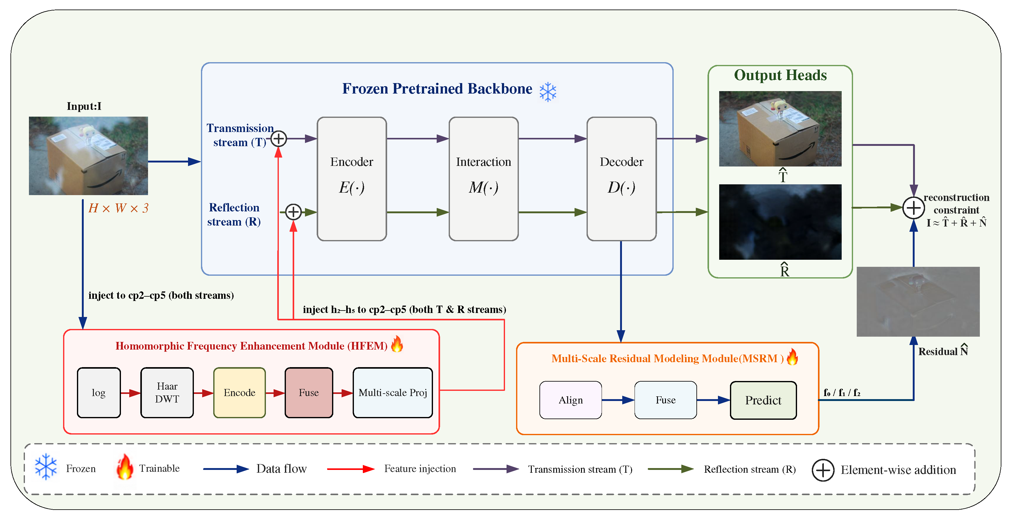
The proposed method is built on a pretrained dual-stream interactive baseline [11], as shown in Figure 1. The baseline separately models transmission and reflection and combines a global prior, local dual-stream priors, and an interactive decoder for layer separation; its detailed structure is given in [11]. We add two structural enhancement modules. HFEM extracts logarithmic-domain frequency features and injects them into corresponding levels of the local dual-stream prior extractor as a complement to conventional spatial features. MSRM acts on the residual-prediction branch and replaces the original single-scale linear residual module. Instead of using only one feature level, MSRM aggregates multiple decoder levels to introduce cross-scale context into nonlinear residual modeling.

During training, all pretrained baseline parameters are frozen, and only HFEM and MSRM are optimized. The complete adapted model contains approximately 328.49 million parameters, while the newly introduced HFEM and MSRM contain approximately 1.528 million trainable parameters in total. Section 3.5 explains this training strategy, and Section 4.4 evaluates it experimentally.

3.3. Homomorphic Frequency Enhancement Module

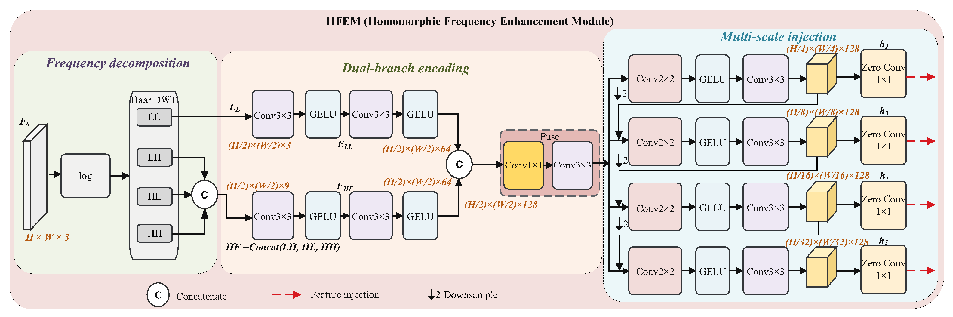
HFEM introduces a logarithmic-domain frequency path into the frozen local dual-stream priors, as shown in Figure 2. It first applies a logarithmic transformation to the input, performs a one-level Haar wavelet decomposition into low- and high-frequency subbands, encodes them through two branches, constructs a multi-scale frequency pyramid, and injects the pyramid into both streams through zero-initialized projections.

3.3.1. Logarithmic-Domain Transformation

Given an input image I, HFEM maps it to the logarithmic domain as

$$x_{\log }=\log \left(\mathrm{clamp}(I,\epsilon )\right).$$

(5)

where $\epsilon$ is a numerical-stability constant that prevents taking the logarithm of zero. As analyzed in Section 3.1, this transformation locally approximates multiplicative coupling in an additive form and provides a statistical representation different from that of the spatial domain. It does not directly separate the two layers.

In the implemented data pipeline, input images are converted to tensors by ToTensor(), resulting in the [0, 1] image-intensity range. For numerical stability, the logarithmic-domain path clamps the input tensor before applying the logarithm. Specifically, HFEM uses torch.log(torch.clamp(x, min = 1 ×10⁻⁴)). This lower bound avoids log(0) and prevents zero or extremely small values from entering the logarithmic operation. The resulting log-domain tensor is then processed by Haar wavelet decomposition and the subsequent learnable convolutional branches. This operation is used as a complementary feature transformation for frequency-domain enhancement, rather than as an analytical separation of transmission and reflection layers.

3.3.2. Haar Wavelet Decomposition

HFEM then applies a one-level Haar discrete wavelet transform [47] to $x_{\log }$:

$$\{LL,LH,HL,HH\}=\mathrm{DWT}\left(x_{\log }\right).$$

(6)

The $LL$ subband represents smooth structures and luminance variation, whereas $LH$, $HL$, and $HH$ represent directional edges and textures. The three high-frequency subbands are concatenated along the channel dimension:

$$HF=\mathrm{Concat}(LH,HL,HH).$$

(7)

3.3.3. Dual-Branch Encoding and Feature Fusion

Because low-frequency structure and high-frequency detail follow different statistics, HFEM encodes $LL$ and $HF$ independently:

$$F_{LL}=E_{LL}\left(LL\right),F_{HF}=E_{HF}\left(HF\right).$$

(8)

The features are then concatenated and fused into a unified logarithmic-domain frequency representation:

$$F_0=\mathrm{Fuse}\left(\mathrm{Concat}(F_{LL},F_{HF})\right).$$

(9)

where $E_{LL}$ and $E_{HF}$ denote the low- and high-frequency encoders, respectively, and Fuse denotes the feature-fusion operator.

3.3.4. Frequency-Feature Pyramid

Because $F_0$ is a single-scale representation, it cannot be injected directly into multiple local-prior levels. HFEM therefore builds a multi-scale pyramid by cascaded downsampling:

$$h_l=D_l\left(h_{l-1}\right),l=2,\dots ,5,h_1=F_0.$$

(10)

where $D_l$ is a downsampling block. The resulting features are aligned scale by scale with the corresponding local-prior levels.

3.3.5. Zero-Initialized Projection and Injection

For the frequency feature at level l, a projection aligns its channels with the target level before it is injected into the transmission and reflection convolutional priors:

$${\widetilde{cp}}_l^T=c{p}_l^T+P_l\left(h_l\right),{\widetilde{cp}}_l^R=c{p}_l^R+P_l\left(h_l\right).$$

(11)

where $c{p}_l^T$ and $c{p}_l^R$ are the convolutional-prior features in the two streams and $P_l$ is the level-specific convolutional projection. Following zero-initialized residual injection [49], the weights and biases of $P_l$ are initialized to zero. Thus $P_l\left(h_l\right)=0$ at initialization. As training proceeds, the projections learn effective frequency complements and inject them into the dual-stream features in residual form. The same frequency prior is injected into both streams because the mixed image’s low-frequency structure and high-frequency detail affect both transmission recovery and reflection estimation.

3.4. Multi-Scale Residual Modeling Module

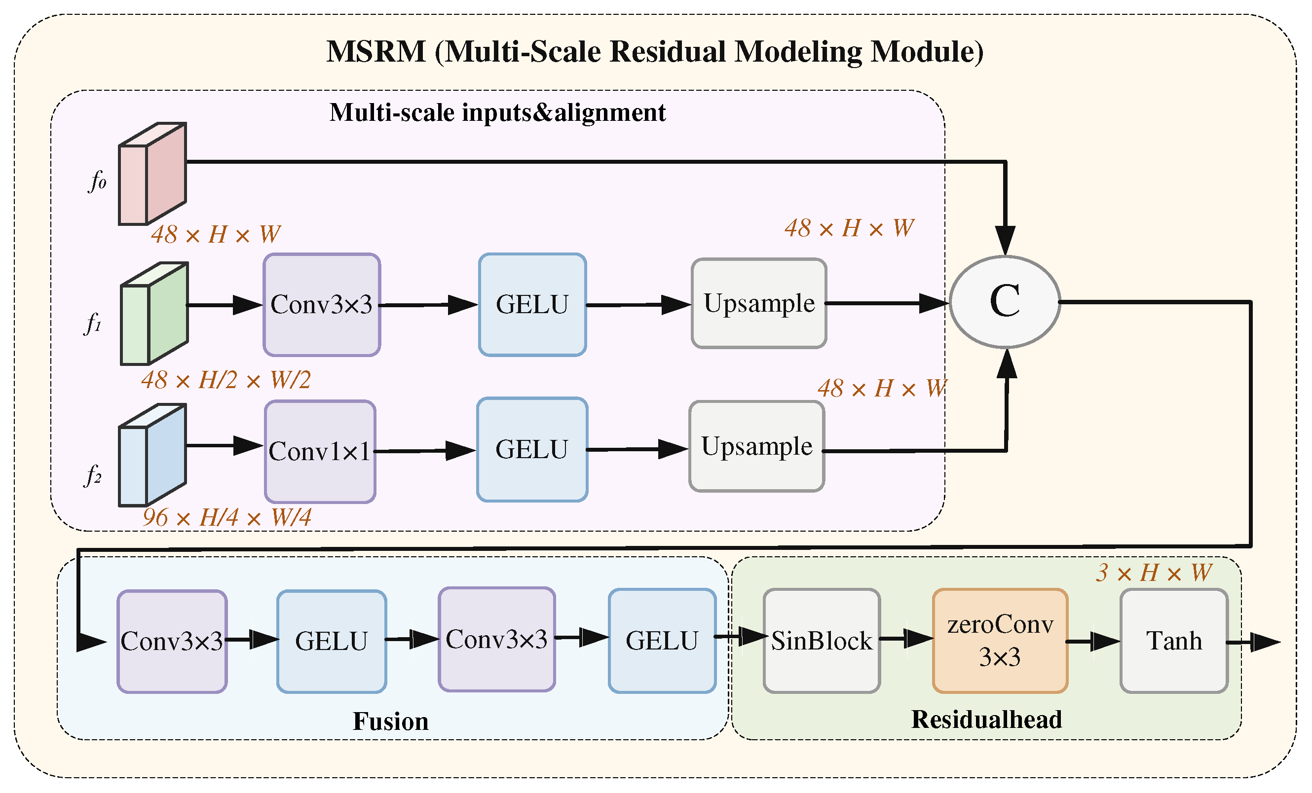
The baseline residual branch predicts nonlinear residuals mainly from a single-scale feature. To accommodate residual variation across spatial scales, MSRM introduces cross-scale context into residual prediction, as illustrated in Figure 3.

Given decoder features $f_0$, $f_1$, and $f_2$ at three levels, MSRM aligns their spatial resolutions and channel dimensions and then fuses them along the channel dimension:

$$F_{\mathrm{ms}}={\mathrm{Fuse}}_{\mathrm{ms}}\left(\mathrm{Align}(f_0,f_1,f_2)\right).$$

(12)

where Align denotes scale and channel alignment, and ${\mathrm{Fuse}}_{\mathrm{ms}}$ denotes multi-scale fusion. This representation provides cross-scale context that is absent when only one decoder level is used.

MSRM directly predicts the residual from the fused representation:

$$\Delta N=\mathrm{Tanh}\left({\mathrm{Conv}}_{\mathrm{zero}}\left(\mathrm{SinBlock}\left(F_{\mathrm{ms}}\right)\right)\right).$$

(13)

where SinBlock retains the basic unit of the baseline residual branch and ${\mathrm{Conv}}_{\mathrm{zero}}$ is a zero-initialized convolution. Since MSRM replaces the original single-scale residual module, zero initialization does not make the entire model strictly identical to the baseline at the beginning of training. It instead sets the initial residual output of MSRM to zero, so that the new branch initially predicts no residual and does not perturb the frozen backbone. MSRM then gradually learns a residual estimate driven by multi-scale features.

Although MSRM does not provide the dominant numerical gain in the ablation study, it is retained because nonlinear residuals in reflection separation are not confined to a single spatial scale. Large-scale residual patterns may arise from smooth attenuation, spatially varying illumination, or broad reflection remnants, whereas small-scale residuals are often related to local highlights, saturation residues, thin reflection edges, and texture leakage. A single-scale residual branch tends to emphasize local responses and may be less effective in jointly modeling these heterogeneous residual patterns. By aggregating decoder features from multiple levels, MSRM provides cross-scale context for residual prediction and serves as a complementary component to HFEM rather than the primary source of improvement.

The ablation results further show that MSRM alone improves the Average494 PSNR by about 0.08 dB, while adding MSRM on top of HFEM brings a further modest improvement of about 0.03 dB. Therefore, MSRM is positioned as a supporting residual-modeling design rather than an equally dominant independent contribution.

3.5. Frozen Training Strategy

When a pretrained model is structurally extended, the training strategy directly affects optimization stability and experimental comparability. We freeze the pretrained dual-stream baseline and optimize only HFEM and MSRM. First, the baseline has already learned stable layer-separation representations for SIRS. Jointly fine-tuning all parameters may allow gradients from the new branches to alter the original feature distribution and weaken the established separation ability [50,51]. Freezing reduces this disturbance. Second, optimization is concentrated on the new modules rather than simultaneously changing the baseline. Because the baseline remains fixed, observed performance changes can also be attributed more directly to the introduced modules, improving the interpretability of ablations and the fairness of training-strategy comparisons.

Although both new modules use zero-initialized connections, replacing the original residual module with MSRM means that the complete model is not strictly equivalent to the baseline at initialization. Section 4.4 evaluates this setting: compared with joint fine-tuning, the frozen strategy produces a smoother training process and fewer performance fluctuations. Prior work has adapted tasks by freezing pretrained weights and optimizing added parameters [52]; related visual-recognition research also reports that restricting the range of parameter updates can outperform full fine-tuning in some settings [53]. These findings motivate our comparison between frozen and joint fine-tuning strategies.

The term frozen baseline means that all original parameters of the pretrained DSIT baseline are kept fixed, and only the newly introduced HFEM and MSRM are optimized. We distinguish three states in this setting. The first is the original pretrained DSIT baseline without architectural modification, which obtains 26.52 dB/0.916 on Average494. The second is the initialized adapted model after replacing the original single-scale residual branch with MSRM. Because the output projection of MSRM is zero-initialized, the initial residual prediction is zero, and the new branch does not disturb the frozen backbone output at the beginning of training. The third is the fully trained adapted model, where HFEM and MSRM have been optimized, and the final model obtains 26.74 dB/0.917. Therefore, the frozen-baseline setting is used as a training strategy for stable adaptation and clearer ablation attribution, rather than as an independent architectural contribution.

3.6. Loss Function

For a fair comparison, we retain the baseline loss settings [11] and introduce no additional supervision. The total loss is

$$\mathcal{L}={\mathcal{L}}_{\mathrm{pix}}+{\mathcal{L}}_{\mathrm{grad}}+{\lambda }_1{\mathcal{L}}_{\mathrm{feat}}+{\lambda }_2{\mathcal{L}}_{\mathrm{rec}}.$$

(14)

where ${\mathcal{L}}_{\mathrm{pix}}$ uses an ${\ell }_2$ norm to constrain pixel errors between predictions and ground truth, ${\mathcal{L}}_{\mathrm{grad}}$ constrains structural differences in the gradient domain and includes a multi-scale gradient-exclusion term [23] to reduce texture leakage, ${\mathcal{L}}_{\mathrm{feat}}$ computes perceptual differences using intermediate features of a pretrained VGG-19 [54,55], and ${\mathcal{L}}_{\mathrm{rec}}$ requires the predicted transmission, reflection, and residual to reconstruct the input. We set ${\lambda }_1=0.01$ and ${\lambda }_2=0.2$.

In our implementation, the perceptual term is computed using a pretrained VGG-19 feature extractor from torchvision, i.e., models.vgg19(pretrained=True).features. The VGG-19 network is kept frozen during training by setting requires_grad=False. Before being fed into VGG-19, the predicted transmission image and the corresponding ground-truth transmission image are normalized using the ImageNet mean and standard deviation, i.e., mean values of [0.485, 0.456, 0.406] and standard deviations of [0.229, 0.224, 0.225]. The perceptual loss is computed as an L1 distance between VGG features extracted at indices [2, 7, 12, 21, 30]. The weight of this term is set to ${\lambda }_{\mathrm{vgg}}=0.01$ in our experiments. This configuration follows the baseline implementation and is kept unchanged for all compared module variants.

Unless otherwise specified, all compared module variants use the same preprocessing pipeline, loss weights, initialization protocol, data augmentation, and optimization settings. Therefore, the ablation comparisons are intended to isolate the effect of the proposed modules under this controlled protocol, rather than to attribute all possible performance differences solely to HFEM and MSRM.

4. Experiments

4.1. Experimental Settings

Datasets. For training, we use the same sirs_dataset protocol as the baseline implementation. The training base directory is DSIT_Data. The training loader constructs approximately 15,000 training image pairs per epoch from three sources: a VOC-based synthetic training set with 7643 images [56], a real training set with 89 images [23], and a nature training set with 200 images [9]. The sampling ratio is set to 0.6/0.2/0.2 for the VOC-based synthetic, real, and nature sources, respectively. For preprocessing, training images are resized and cropped to a fixed size of 384 × 384, with random horizontal flipping enabled. During testing, the model is evaluated on five public benchmarks, namely Real20 [23], Object200, Postcard199, Wild55, and Nature20; Object200, Postcard199, and Wild55 are from the SIR² dataset [57]. Average494 is computed as the weighted average over all 494 test images.

Implementation details. For implementation, we use the officially released Setting 2 pretrained weights of the baseline model at epoch 66 and adopt the dsit_homo_large architecture. During training, all original baseline parameters are frozen, and only the newly introduced HFEM and MSRM are optimized. Adam is used as the optimizer [58] with a fixed learning rate of $1\times {10}^{-4}$ and a batch size of 1. The model is trained for 50 epochs, corresponding to approximately 750,000 optimization steps with approximately 15,000 training image pairs per epoch. The loss weights are set to ${\lambda }_{\mathrm{vgg}}=0.01$ and ${\lambda }_{\mathrm{rec}}=0.2$. All experiments are conducted on a single NVIDIA RTX 3090 GPU.

To address possible data leakage between training and testing data, we performed a two-stage check. First, a global filename-level scan between the training and test directories found eight numeric file names that appear in both. Second, for these eight shared names, we compared both the raw-file MD5 and the decoded pixel-level MD5 of the corresponding images. No pair among the eight shared names had an identical raw-file hash or an identical pixel-level hash. This indicates that the shared names are caused by generic numeric file naming rather than by identical image content, and that no identical training image was found in the test sets under this check.

Evaluation metrics. Peak signal-to-noise ratio (PSNR) and structural similarity (SSIM) are used to evaluate the recovered transmission layer. For methods evaluated by us, the same test images and metric computation are used. For DMDNet, the per-dataset results are cited from the original paper, and the Average494 value is recomputed using the same image-count-weighted protocol. Average494 is weighted by the number of images in Real20, Object200, Postcard199, Wild55, and Nature20.

4.2. Quantitative Comparison

Table 2. Quantitative comparison of PSNR (dB) and SSIM on five benchmark datasets. Bold and underlined values indicate the best and second-best results, respectively.

Method	Venue	Real20		Object200		Postcard199		Wild55		Nature20		Average494		Average5
		PSNR	SSIM	PSNR	SSIM	PSNR	SSIM	PSNR	SSIM	PSNR	SSIM	PSNR	SSIM	PSNR	SSIM
ERRNet † [7]	CVPR’19	22.69	0.803	24.91	0.896	20.78	0.876	25.33	0.853	23.08	0.756	23.13	0.873	23.36	0.837
IBCLN † [9]	CVPR’20	21.86	0.750	24.87	0.884	23.39	0.871	24.71	0.878	23.57	0.763	24.08	0.868	23.68	0.829
YTMT † [12]	NeurIPS’21	23.26	0.810	24.87	0.898	22.91	0.864	25.48	0.888	23.85	0.818	24.05	0.877	24.07	0.856
DSRNet † [4]	ICCV’23	24.23	0.821	26.28	0.921	24.56	0.904	25.68	0.922	25.22	0.844	25.40	0.908	25.19	0.882
Robust † [26]	CVPR’23	23.61	0.835	24.90	0.917	19.91	0.868	23.67	0.884	20.97	0.764	22.54	0.884	22.61	0.854
RRW † [8]	CVPR’24	23.82	0.817	26.55	0.927	24.03	0.903	26.51	0.913	25.96	0.843	25.40	0.908	25.37	0.881
DSIT † [11]	NeurIPS’24	24.91	0.831	26.82	0.922	26.00	0.924	27.89	0.921	26.60	0.843	26.52	0.916	26.44	0.888
RDNet † [28]	CVPR’25	24.83	0.840	26.94	0.923	25.87	0.920	27.58	0.913	26.71	0.851	26.48	0.914	26.39	0.889
DExNet † [30]	TPAMI’25	23.50	0.817	26.38	0.916	25.52	0.918	26.95	0.908	24.66	0.837	25.91	0.909	25.40	0.879
DMDNet ‡ [59]	AAAI’26	24.60	0.836	27.07	0.929	25.32	0.921	27.70	0.920	26.68	0.838	26.32	0.917	26.27	0.889
Ours	–	24.96	0.828	27.21	0.927	26.05	0.921	28.06	0.923	26.99	0.845	26.74	0.917	26.65	0.889

^† Results are evaluated by us using publicly available implementations and released checkpoints when available, under a unified evaluation protocol with the same test images and metric computation. Model-specific preprocessing follows the corresponding public implementation. ^‡ For DMDNet, the per-dataset PSNR/SSIM values are cited from the original DMDNet paper. Since the original paper reports a different averaging protocol, we recompute the Average494 value using the same image-count-weighted protocol as the other methods for a consistent presentation. Because these per-dataset values are taken from the original paper rather than evaluated by us under the same implementation protocol, the DMDNet result should be interpreted as a reference comparison.

compares the proposed method with representative SIRS methods on five test sets using PSNR and SSIM. The methods cover single-stream restoration, dual-stream reconstruction, and dual-stream interaction. Average494 is the image-count-weighted average over all 494 test images. For a fair comparison, ERRNet, IBCLN, YTMT, DSRNet, Robust, RRW, DSIT, RDNet, and DExNet are evaluated by us using publicly available implementations and released checkpoints when available, with the same test images and metric computation. For DMDNet, whose per-dataset results are cited from the original paper, the weighted Average494 value is recomputed using the image-count-weighted protocol for consistency and is provided as a reference comparison.

To verify that the improvement is not dominated by the two largest datasets, Object200 and Postcard199, we also report Average5, i.e., the unweighted arithmetic mean over the five benchmarks. Under Average5, the proposed method improves PSNR from 26.44 dB to 26.65 dB (+0.21 dB), which is consistent with the +0.22 dB gain under the image-count-weighted Average494. This suggests that the observed improvement is not solely caused by the image-count weighting scheme.

To examine whether the modest improvement is affected by random-seed variation, we further train the complete model with three different random seeds under the same training and evaluation settings. As shown in

Table 3. Multi-seed stability of the proposed method on Average494 over three independent runs with different random seeds.

Run (Seed)	Average494 PSNR	Average494 SSIM
Seed 1	26.74	0.917
Seed 2	26.73	0.917
Seed 3	26.77	0.917
Mean ± std	26.75 ± 0.02	0.917 ± 0.000

, the Average494 PSNR values of the three runs are 26.74 dB, 26.73 dB, and 26.77 dB, respectively, yielding a mean value of 26.75 dB with a standard deviation of 0.02 dB. The rounded SSIM values remain stable at 0.917 for all three runs. Compared with the DSIT baseline result of 26.52 dB/0.916, the main Table 2 result improves PSNR by 0.22 dB, while the multi-seed mean improves PSNR by 0.23 dB. This improvement is well above the seed-level variation and is unlikely to be explained by random seed variation alone. Nevertheless, we keep the description conservative and regard the overall gain as modest but reproducible.

Overall, the proposed method achieves 26.74 dB/0.917 on Average494. Relative to the DSIT baseline at 26.52 dB/0.916, PSNR increases by 0.22 dB and SSIM by 0.001. Although the average gain is limited, HFEM and MSRM still provide an overall benefit while the baseline remains frozen.

The PSNR gains are more evident on Object200, Wild55, and Nature20. Object200 improves from 26.82 to 27.21 dB, Wild55 from 27.89 to 28.06 dB, and Nature20 from 26.60 to 26.99 dB, with the latter reaching the best result on that dataset. On Real20 and Postcard199, the method still improves over the baseline, from 24.91 to 24.96 dB and from 26.00 to 26.05 dB, respectively, but by smaller margins. This difference suggests that the benefit of frequency enhancement depends on the data distribution. When the transmission layer contains abundant high-frequency texture, high-frequency responses may originate from both transmission and reflection and overlap in the frequency domain, reducing the complementary value of the frequency features. Section 4.5 analyzes this behavior further.

The SSIM behavior is consistent with PSNR. The proposed method obtains 0.927, 0.923, and 0.845 on Object200, Wild55, and Nature20, respectively, with the best value in the table on Wild55. In summary, PSNR increases on all five test sets, SSIM improves on some sets, and the gain depends on transmission texture, reflection strength, and frequency overlap between the layers.

4.3. Ablation Study

To provide a more detailed ablation analysis, we extend the original Average494-only ablation table to a per-dataset comparison, as shown in

Table 4. Per-dataset ablation of the proposed modules on the five benchmarks. Average494 is the image-count-weighted average over all 494 test images. Average5 denotes the unweighted arithmetic mean over the five benchmarks. Bold values highlight the Average494 and Average5 results of the full model.

Configuration	Real20		Object200		Postcard199		Wild55		Nature20		Average494		Average5
	PSNR	SSIM	PSNR	SSIM	PSNR	SSIM	PSNR	SSIM	PSNR	SSIM	PSNR	SSIM	PSNR	SSIM
w/o HFEM & MSRM	24.91	0.831	26.82	0.922	26.00	0.924	27.89	0.921	26.60	0.843	26.52	0.916	26.44	0.888
w/o HFEM	24.96	0.829	27.08	0.925	25.93	0.921	27.82	0.921	26.87	0.844	26.60	0.916	26.53	0.888
w/o MSRM	24.96	0.831	27.09	0.925	26.17	0.923	27.83	0.922	26.95	0.844	26.71	0.917	26.60	0.889
Ours	24.96	0.828	27.21	0.927	26.05	0.921	28.06	0.923	26.99	0.845	26.74	0.917	26.65	0.889

. The results show that HFEM is the primary source of the overall gain, improving the weighted Average494 PSNR from 26.52 dB to 26.71 dB. In contrast, MSRM alone provides a smaller improvement, reaching 26.60 dB. When HFEM and MSRM are combined, the full model obtains 26.74 dB/0.917 on Average494, indicating a limited but positive additional gain over HFEM alone. The per-dataset results also show that the improvements are not uniform across benchmarks. The full model shows clearer gains on Object200, Wild55, and Nature20, while the changes on Real20 and Postcard199 are smaller and show slight fluctuations compared with HFEM alone. Specifically, the full model obtains 24.96 dB on Real20 and 26.05 dB on Postcard199; the latter is lower than the 26.17 dB obtained with HFEM alone. This observation is consistent with the dataset-distribution analysis in Section 4.5 and suggests that the benefit of frequency enhancement and residual modeling depends on the reflection characteristics of each benchmark.

The Average5 results in Table 4 show the same trend as Average494: HFEM provides the main improvement, MSRM alone provides a smaller gain, and the full model obtains the best unweighted PSNR of 26.65 dB.

We further conduct two auxiliary ablations to examine the logarithmic transformation in HFEM and the initialization of the injection projections. As shown in

Table 5. Ablation on the logarithmic transformation and the projection initialization on Average494.

Setting	Average494 PSNR	Observation
HFEM w/o log	26.63	Removing the logarithmic transformation from HFEM
Random-init projection	26.73	Replacing zero-initialized projections with random initialization
Ours (with log, zero-init)	26.74	Full setting

, removing the logarithmic transformation from HFEM decreases the Average494 PSNR from 26.71 dB to 26.63 dB, indicating that the logarithmic-domain transformation provides a positive contribution to the proposed frequency-enhancement path. This result supports the effectiveness of using the log-domain representation as a complementary feature transformation, but it does not imply that the logarithmic domain analytically separates reflection.

For projection initialization, replacing the zero-initialized projections with random initialization obtains 26.73 dB on Average494, which is very close to the 26.74 dB of the full zero-initialized model. Therefore, zero initialization does not mainly contribute by increasing the final PSNR in this experiment. Its role is to make the newly added injection branches output zero at the beginning of training, so that the frozen pretrained backbone is not immediately disturbed by random injected features. The random-initialized variant can reach a similar final performance, but zero initialization provides a smoother and safer way to connect the added frequency path to the frozen baseline.

4.4. Training-Strategy Analysis

To evaluate the effect of freezing on optimization stability,

Table 6. Stability comparison of different training strategies.

Strategy	Average Range (dB)	Fluctuation (dB)	Performance Drop
Not frozen	23.00–26.65	3.65	Yes
Frozen (ours)	26.46–26.74	0.28	No

compares frozen and non-frozen training. The non-frozen strategy jointly updates both the pretrained baseline and the newly introduced modules using the same learning rate of $1\times {10}^{-4}$ as in the frozen setting; all other settings match Section 4.1. This setting avoids introducing an additional group-specific learning-rate schedule, but it should not be interpreted as an exhaustive hyperparameter search over all possible joint fine-tuning configurations.

During training, the weighted Average494 PSNR is evaluated once per epoch. In Table 6, “Average range” denotes the minimum-to-maximum span of the epoch-wise Average494 PSNR values, and “Fluctuation” is computed as the difference between the maximum and minimum values in this span.

The two strategies differ substantially in stability. With joint updating, weighted-average PSNR fluctuates over a 3.65 dB range and undergoes several sharp drops. With freezing, it remains between 26.46 and 26.74 dB, a range of only 0.28 dB, and converges without sharp degradation. This agrees with the analysis in Section 3.5: freezing prevents disruption of the pretrained representation. The frozen strategy does not underperform the non-frozen setting in final performance and has clear advantages in stability and reproducibility, so it is adopted in the final model.

4.5. Dataset Response Difference Analysis

The gains vary across datasets. A notable pattern is their relationship with the high-frequency texture intensity of the transmission layer. In Object200 and Nature20, the transmitted content mainly comprises structured objects or natural scenes with relatively regular edges and textures; the high-frequency wavelet subbands therefore capture scene structure clearly, and HFEM provides an effective complement. In Postcard199, the transmitted content is printed imagery rich in high-frequency texture. Its intrinsic high frequencies overlap strongly with those introduced by reflection, making the two components more difficult to distinguish in the frequency domain and reducing the marginal gain of HFEM.

Real20 contains only 20 test images, so its metrics are sensitive to individual samples; the small gain of approximately 0.05 dB is also influenced by sample size. Overall, frequency enhancement does not produce equal gains for all data distributions. It is more helpful when transmission structures are comparatively clear and less helpful when the transmission itself contains very strong high-frequency texture. This observation clarifies the scope of frequency modeling and suggests that future datasets and methods should consider the frequency-domain separability of transmission and reflection.

4.6. Qualitative Comparison

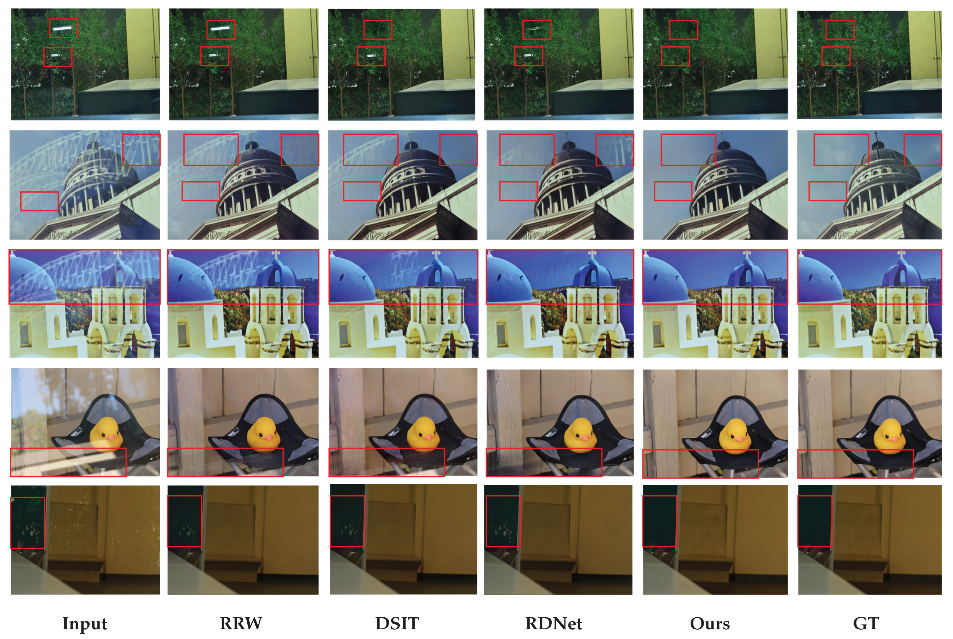
In addition to quantitative metrics, Figure 4 presents a qualitative comparison on representative samples from the Real and SIR² datasets. The comparison includes RRW, DSIT, and RDNet, and red boxes identify regions with visible reflection remnants, local artifacts, or structural differences.

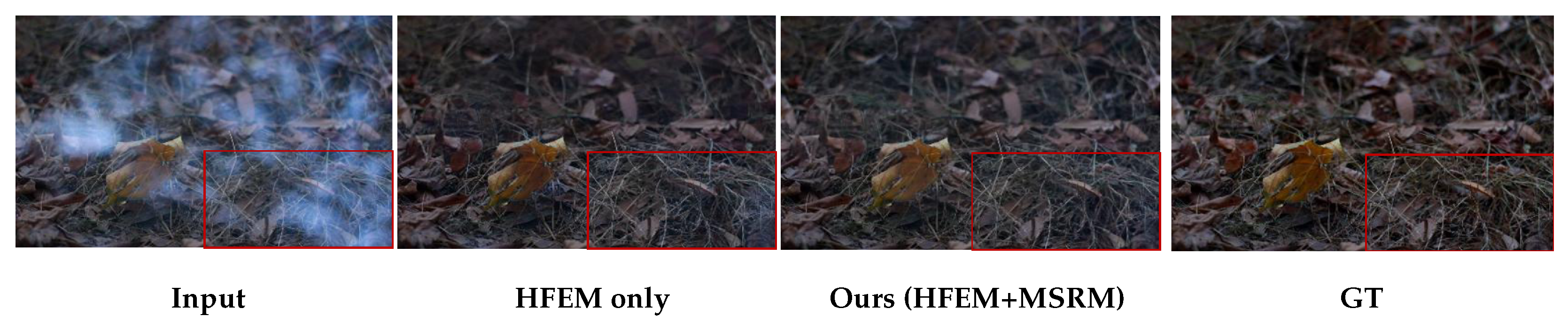
Figure 5 provides a qualitative ablation example for the interaction between HFEM and MSRM. Although the numerical gain of adding MSRM to HFEM is modest, HFEM alone can still leave weak residual reflection traces in some local regions. By aggregating multi-level decoder features, MSRM further suppresses these residual artifacts and provides complementary residual refinement after frequency enhancement. This observation supports our revised positioning of MSRM as a complementary residual-modeling component rather than the primary source of improvement.

Existing methods can retain reflection interference in complex scenes. In regions containing strong light or small bright points, competing methods often preserve noticeable highlights or local blur. In areas with structured reflection, linear reflection patterns remain entangled with the background, while removing tree shadows or foreground-light reflections can introduce red or black artifacts. The proposed method suppresses these remnants more effectively, reduces highlights and structural traces, and better maintains local color and structural consistency. These observations are consistent with Table 2.

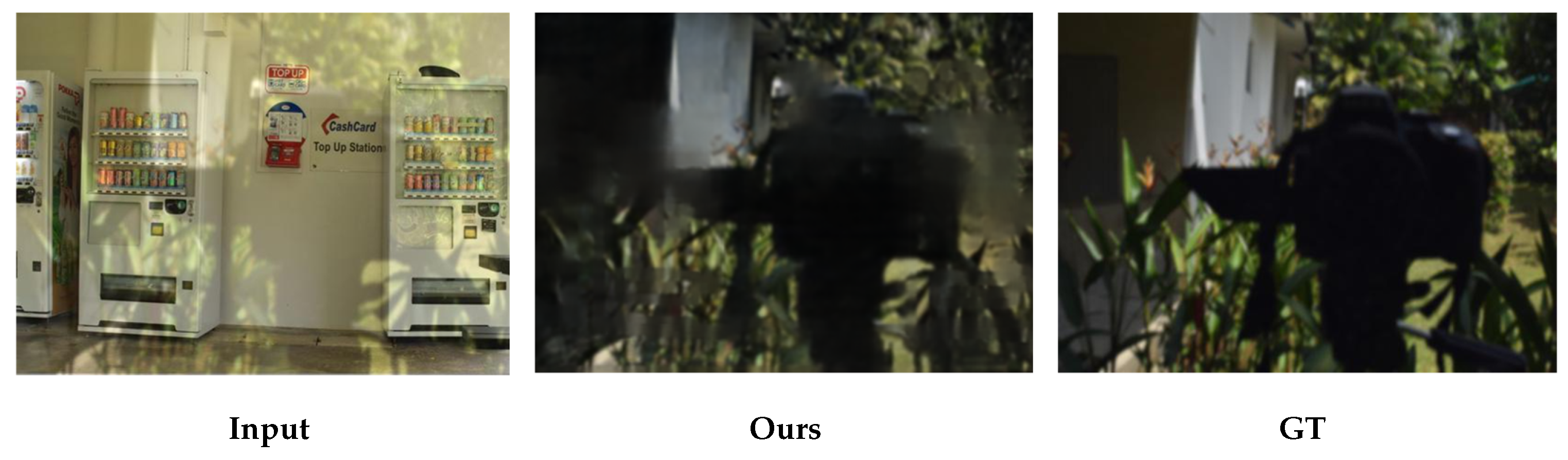
Figure 6 further shows predicted reflection layers. The predictions capture major reflection structures such as plant outlines, local shadows, and spatial luminance distributions, and their overall shapes resemble the corresponding ground truth. Thus, the dual-stream framework not only restores transmission but also constructs a reasonable reflection representation, with the two layers jointly supporting separation.

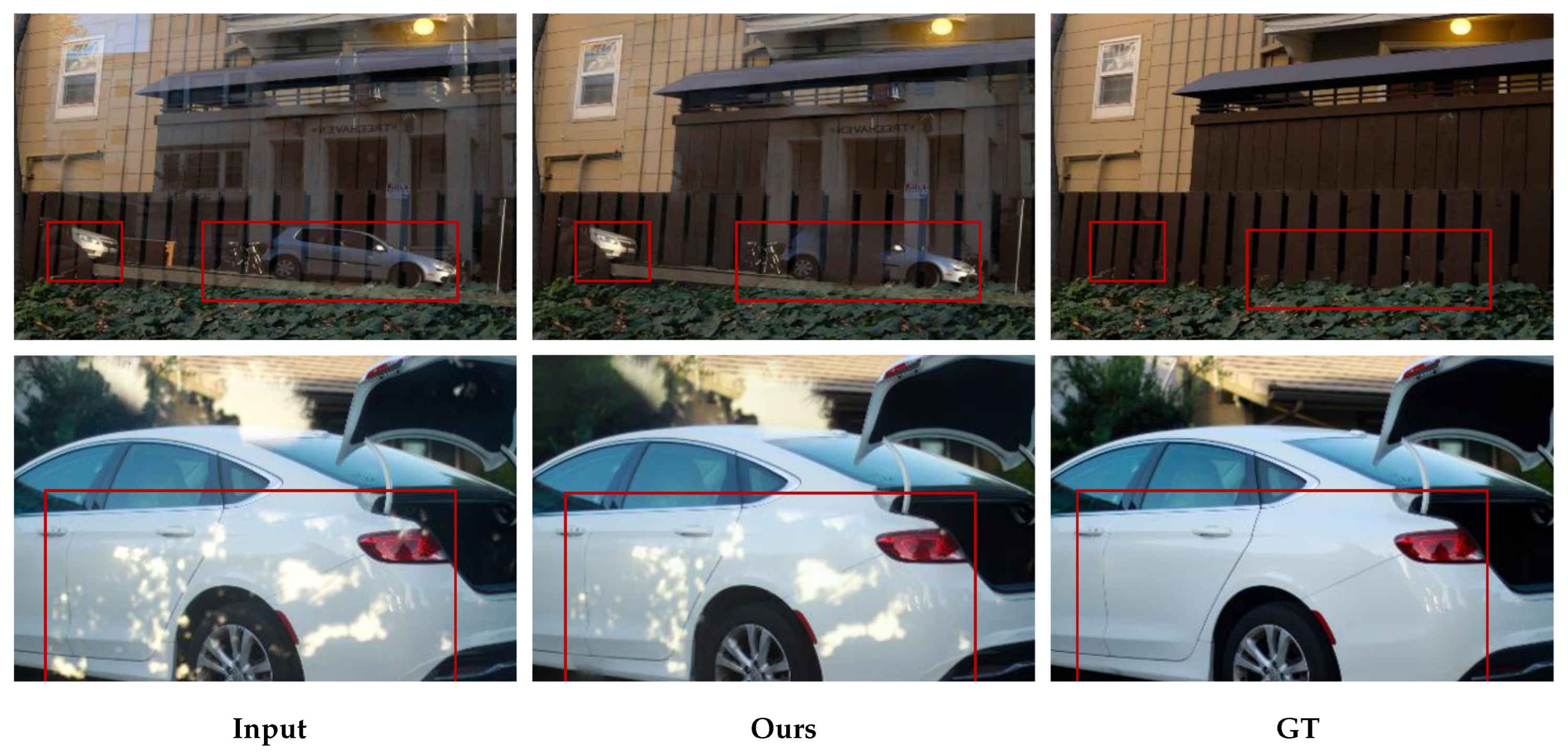
Figure 7 shows two representative failure cases on challenging real-world scenes. These examples contain strong structured reflections, challenging illumination, or high-frequency transmission textures, where the reflection components overlap with the transmission content in the frequency domain. In such cases, the proposed method can still leave visible reflection residues in local regions, as marked by the red boxes. In the first row, reflected objects across the wall and fence remain partially visible, while in the second row, reflected light patterns on the vehicle body are not completely removed. This observation is consistent with the dataset-response analysis in Section 4.5: when the high-frequency components of the transmission and reflection layers are strongly entangled, the complementary frequency information provided by HFEM becomes less discriminative, which limits residual suppression. These failure cases further indicate that the benefit of the proposed method depends on the frequency-domain separability of the two layers and motivate future adaptive frequency modeling to better distinguish high-frequency transmission textures from high-frequency reflection artifacts.

4.7. Complexity Analysis

The parameter efficiency discussed in this work primarily refers to the number of parameters optimized during training. Only HFEM and MSRM are trainable, comprising 1.528 M newly introduced parameters, or 0.47% of the 328.49 M-parameter complete model. The newly introduced modules are therefore small in terms of trainable parameters; this statement does not imply that the inference computation of the complete model is substantially reduced.

The pretrained baseline remains frozen during optimization but still participates in the complete forward computation at inference. In particular, the pretrained swin_prior backbone contains 195.20 M frozen parameters. Accordingly, the FLOPs, MACs, peak GPU memory, latency, and throughput reported in

Table 7. Complexity analysis measured on an NVIDIA RTX 3090 with a 384 × 384 input, batch size = 1, and FP32.

Metric	Value	Scope
Complete-model parameters	328.49 M	Complete model
Frozen swin_prior parameters	195.20 M	Pretrained backbone
HFEM trainable parameters	1.318 M	Added module
MSRM trainable parameters	0.210 M	Added module
HFEM+MSRM trainable parameters	1.528 M	0.47% of complete model
Complete-model FLOPs	1102.72 GFLOPs	Complete forward pass
Complete-model MACs	551.36 GMACs	Complete forward pass
Peak GPU memory	2851 MB	Complete model
Latency	235.87 ms/image	Complete model
Throughput	4.24 FPS	Complete model

are measured for the complete model, including the baseline, HFEM, and MSRM.

The added modules introduce additional computation through the logarithmic transformation, Haar discrete wavelet transform, multi-scale frequency-pyramid construction, and multi-scale residual feature alignment. This overhead is relatively small within the 328.49 M-parameter adapted architecture, and the main computational cost still originates from the pretrained dual-stream baseline.

All complexity measurements use a 384 × 384 input with batch size = 1 on an NVIDIA RTX 3090 under FP32 and evaluation mode. Latency is averaged over 50 runs after 10 warmup runs. Inference speed and peak memory depend on the hardware platform and implementation details.

5. Conclusions

In this paper, we presented a structural enhancement method for a pretrained dual-stream baseline for single-image reflection separation. The proposed HFEM introduces logarithmic-domain Haar wavelet features as complementary frequency-domain information and injects them into the local-prior branches of both streams, while MSRM replaces the original single-scale residual module with a multi-scale residual-modeling design. During training, the pretrained baseline is kept frozen, and only the newly introduced modules are optimized. On five public benchmarks with 494 images in total, the proposed method improves the weighted-average PSNR/SSIM from 26.52 dB/0.916 to 26.74 dB/0.917, corresponding to modest increases of 0.22 dB in PSNR and 0.001 in SSIM. The overall gain is limited in magnitude, but the results show that the proposed structural enhancement can provide a consistent benefit for the frozen pretrained baseline. The final implementation introduces 1.528 M additional trainable parameters, including 1.318 M from HFEM and 0.210 M from MSRM, accounting for approximately 0.47% of the complete 328.49 M-parameter adapted model. In addition, the frozen-baseline training setting shows a more stable optimization process, with a PSNR fluctuation of 0.28 dB compared with 3.65 dB for joint fine-tuning. This setting is used as a training strategy for stable adaptation and clearer ablation attribution rather than as an independent architectural contribution.

Several limitations remain. Although the proposed method improves the weighted Average494 PSNR from 26.52 dB to 26.74 dB, corresponding to a gain of 0.22 dB, the overall improvement is modest and varies across datasets. In particular, when the transmission layer contains strong high-frequency textures that overlap with reflection artifacts in the frequency domain, the complementary benefit of HFEM may be reduced. The logarithmic-domain transformation is used as a complementary feature transformation motivated by local homomorphic analysis rather than as a strict image-wide analytical decomposition of transmission and reflection layers. The ablation results also indicate that HFEM is the main architectural contribution, whereas MSRM provides a smaller complementary residual-modeling benefit. In addition, the current analysis does not include a parameter-matched spatial control module with a similar number of trainable parameters. Such a comparison would further help isolate the effect of logarithmic-domain frequency modeling from the effect of additional trainable capacity. The discussion of frequency overlap in this work is mainly qualitative; future work will define measurable texture or frequency-overlap indicators and analyze their relationship with image-level and dataset-level performance variations.

The quantitative evaluation in this paper focuses on the recovered transmission layer using PSNR and SSIM, while the reflection layer is mainly shown qualitatively because most real-world benchmarks used in this study do not provide reliable reflection-layer ground truth. When suitable datasets with reflection-layer annotations become available, we plan to include reflection-layer quantitative evaluation to more comprehensively assess the dual-stream separation ability. Future work will also include controlled synthetic studies and systematic failure-case analysis under different reflection strengths, blur levels, spatially varying transmittance, saturation, and high-frequency transmission textures. These analyses will support the development of adaptive frequency modeling strategies that can better distinguish high-frequency transmission textures from high-frequency reflection artifacts.

Future work will also examine parameter-matched spatial controls, shared versus independent frequency injection, alternative wavelet bases and decomposition levels, broader fine-tuning strategies, per-image distribution and median analyses, and error or residual-map evaluation when suitable annotations and computational resources are available.

References

1. Wan, R.; Shi, B.; Li, H.; Duan, L.-Y.; Tan, A.-H.; Kot, A.C. Reflection scene separation from a single image. In Proceedings of the IEEE/CVF Conference on Computer Vision and Pattern Recognition; IEEE: New York, NY, USA, 2020; pp. 2398–2406. [Google Scholar]
2. Wieschollek, P.; Gallo, O.; Gu, J.; Kautz, J. Separating reflection and transmission images in the wild. In Proceedings of the European Conference on Computer Vision; Springer: Cham, Switzerland, 2018; pp. 89–104. [Google Scholar]
3. Gong, J.; Xu, J.; Sun, H. Dual-channel blind image separation based on a wavelet suppression interactive diffusion model. J. Image Graph. 2026, 31, 465–478. [Google Scholar] [CrossRef] [Scilit]
4. Hu, Q.; Guo, X. Single image reflection separation via component synergy. In Proceedings of the IEEE/CVF International Conference on Computer Vision; IEEE: New York, NY, USA, 2023; pp. 13138–13147. [Google Scholar]
5. Li, Y.; Brown, M.S. Single image layer separation using relative smoothness. In Proceedings of the IEEE Conference on Computer Vision and Pattern Recognition; IEEE: New York, NY, USA, 2014; pp. 2752–2759. [Google Scholar]
6. Shih, Y.; Krishnan, D.; Durand, F.; Freeman, W.T. Reflection removal using ghosting cues. In Proceedings of the IEEE Conference on Computer Vision and Pattern Recognition; IEEE: New York, NY, USA, 2015; pp. 3193–3201. [Google Scholar]
7. Wei, K.; Yang, J.; Fu, Y.; Wipf, D.; Huang, H. Single image reflection removal exploiting misaligned training data and network enhancements. In Proceedings of the IEEE/CVF Conference on Computer Vision and Pattern Recognition; IEEE: New York, NY, USA, 2019; pp. 8178–8187. [Google Scholar]
8. Zhu, Y.; Fu, X.; Jiang, P.-T.; Zhang, H.; Sun, Q.; Chen, J.; Zha, Z.-J.; Li, B. Revisiting single image reflection removal in the wild. In Proceedings of the IEEE/CVF Conference on Computer Vision and Pattern Recognition; IEEE: New York, NY, USA, 2024; pp. 25468–25478. [Google Scholar]
9. Li, C.; Yang, Y.; He, K.; Lin, S.; Hopcroft, J.E. Single image reflection removal through cascaded refinement. In Proceedings of the IEEE/CVF Conference on Computer Vision and Pattern Recognition; IEEE: New York, NY, USA, 2020; pp. 3565–3574. [Google Scholar]
10. Yang, J.; Gong, D.; Liu, L.; Shi, Q. Seeing deeply and bidirectionally: A deep learning approach for single image reflection removal. In Proceedings of the European Conference on Computer Vision; Springer: Cham, Switzerland, 2018; pp. 654–669. [Google Scholar]
11. Hu, Q.; Wang, H.; Guo, X. Single image reflection separation via dual-stream interactive transformers. In Proceedings of Neural Information Processing Systems; Curran Associates, Inc.: Red Hook, NY, USA, 2024; Volume 37, pp. 55228–55248. [Google Scholar]
12. Hu, Q.; Guo, X. Trash or treasure? An interactive dual-stream strategy for single image reflection separation. In Proceedings of Neural Information Processing Systems; Curran Associates, Inc.: Red Hook, NY, USA, 2021; Volume 34, pp. 24683–24694. [Google Scholar]
13. Dong, Z.; Xu, K.; Yang, Y.; Bao, H.; Xu, W.; Lau, R.W.H. Location-aware single image reflection removal. In Proceedings of the IEEE/CVF International Conference on Computer Vision; IEEE: New York, NY, USA, 2021; pp. 5017–5026. [Google Scholar]
14. Oppenheim, A.V.; Schafer, R.W.; Stockham, T.G. Nonlinear filtering of multiplied and convolved signals. Proc. IEEE 1968, 56, 1264–1291. [Google Scholar] [CrossRef] [Scilit]
15. Gonzalez, R.C.; Woods, R.E. Digital Image Processing, 4th ed.; Pearson: London, UK, 2018. [Google Scholar]
16. Zamir, S.W.; Arora, A.; Khan, S.; Hayat, M.; Khan, F.S.; Yang, M.-H.; Shao, L. Learning enriched features for real image restoration and enhancement. In Proceedings of the European Conference on Computer Vision; Springer: Cham, Switzerland, 2020; pp. 492–511. [Google Scholar]
17. Zamir, S.W.; Arora, A.; Khan, S.; Hayat, M.; Khan, F.S.; Yang, M.-H.; Shao, L. Multi-stage progressive image restoration. In Proceedings of the IEEE/CVF Conference on Computer Vision and Pattern Recognition; IEEE: New York, NY, USA, 2021; pp. 14821–14831. [Google Scholar]
18. Wang, Z.; Cun, X.; Bao, J.; Zhou, W.; Liu, J.; Li, H. Uformer: A general U-shaped Transformer for image restoration. In Proceedings of the IEEE/CVF Conference on Computer Vision and Pattern Recognition; IEEE: New York, NY, USA, 2022; pp. 17683–17693. [Google Scholar]
19. Arvanitopoulos, N.; Achanta, R.; Süsstrunk, S. Single image reflection suppression. In Proceedings of the IEEE Conference on Computer Vision and Pattern Recognition; IEEE: New York, NY, USA, 2017; pp. 4498–4506. [Google Scholar]
20. Levin, A.; Weiss, Y. User assisted separation of reflections from a single image using a sparsity prior. IEEE Trans. Pattern Anal. Mach. Intell. 2007, 29, 1647–1654. [Google Scholar] [CrossRef] [Scilit] [PubMed]
21. Wan, R.; Shi, B.; Duan, L.-Y.; Tan, A.-H.; Kot, A.C. CRRN: Multi-scale guided concurrent reflection removal network. In Proceedings of the IEEE Conference on Computer Vision and Pattern Recognition; IEEE: New York, NY, USA, 2018; pp. 4777–4785. [Google Scholar]
22. Fan, Q.; Yang, J.; Hua, G.; Chen, B.; Wipf, D. A generic deep architecture for single image reflection removal and image smoothing. In Proceedings of the IEEE International Conference on Computer Vision; IEEE: New York, NY, USA, 2017; pp. 3238–3247. [Google Scholar]
23. Zhang, X.; Ng, R.; Chen, Q. Single image reflection separation with perceptual losses. In Proceedings of the IEEE Conference on Computer Vision and Pattern Recognition; IEEE: New York, NY, USA, 2018; pp. 4786–4794. [Google Scholar]
24. Liu, Z.; Lin, Y.; Cao, Y.; Hu, H.; Wei, Y.; Zhang, Z.; Lin, S.; Guo, B. Swin Transformer: Hierarchical vision transformer using shifted windows. In Proceedings of the IEEE/CVF International Conference on Computer Vision; IEEE: New York, NY, USA, 2021; pp. 10012–10022. [Google Scholar]
25. Deng, J.; Dong, W.; Socher, R.; Li, L.-J.; Li, K.; Fei-Fei, L. ImageNet: A large-scale hierarchical image database. In Proceedings of the IEEE Conference on Computer Vision and Pattern Recognition; IEEE: New York, NY, USA, 2009; pp. 248–255. [Google Scholar]
26. Song, Z.; Zhang, Z.; Zhang, K.; Luo, W.; Fan, Z.; Ren, W.; Lu, J. Robust single image reflection removal against adversarial attacks. In Proceedings of the IEEE/CVF Conference on Computer Vision and Pattern Recognition; IEEE: New York, NY, USA, 2023; pp. 24688–24698. [Google Scholar]
27. Chen, Y.; He, Z.; Liu, X.; Chen, Z.; Lu, Z.-M. GFRRN: Explore the Gaps in Single Image Reflection Removal. In Proceedings of the IEEE/CVF Conference on Computer Vision and Pattern Recognition; IEEE: New York, NY, USA, 2026; pp. 5690–5699. [Google Scholar]
28. Zhao, H.; Li, M.; Hu, Q.; Guo, X. Reversible decoupling network for single image reflection removal. In Proceedings of the 2025 IEEE/CVF Conference on Computer Vision and Pattern Recognition (CVPR); IEEE: New York, NY, USA, 2025; pp. 26430–26439. [Google Scholar]
29. Huang, J.-J.; Liu, T.; Xia, J.; Wang, M.; Dragotti, P.L. DURRNet: Deep unfolded single image reflection removal network with joint prior. In Proceedings of the IEEE International Conference on Acoustics, Speech and Signal Processing; IEEE: New York, NY, USA, 2024; pp. 5235–5239. [Google Scholar]
30. Huang, J.-J.; Liu, T.; Chen, Z.; Liu, X.; Wang, M.; Dragotti, P.L. A lightweight deep exclusion unfolding network for single image reflection removal. IEEE Trans. Pattern Anal. Mach. Intell. 2025, 47, 4957–4973. [Google Scholar] [CrossRef] [Scilit] [PubMed]
31. Chen, X.; Jiang, X.; Tao, Y.; Lei, Z.; Li, Q.; Lei, C.; Zhang, Z. FIRM: Flexible interactive reflection ReMoval. In Proceedings of the AAAI Conference on Artificial Intelligence; AAAI Press: Washington, DC, USA, 2025; pp. 2230–2238. [Google Scholar]
32. Kee, E.; Pikielny, A.; Blackburn-Matzen, K.; Levoy, M. Removing reflections from RAW photos. In Proceedings of the IEEE/CVF Conference on Computer Vision and Pattern Recognition; IEEE: New York, NY, USA, 2025; pp. 161–171. [Google Scholar]
33. Yang, K.; Cai, J.; Ouyang, L.; Vasluianu, F.A.; Timofte, R.; Ding, J.; Sun, H.; Fu, L.; Li, J.; Ho, C.M.; et al. NTIRE 2025 challenge on single image reflection removal in the wild: Datasets, methods and results. In Proceedings of the IEEE/CVF Conference on Computer Vision and Pattern Recognition Workshops; IEEE: New York, NY, USA, 2025; pp. 1301–1311. [Google Scholar]
34. Yin, W.; Zhang, J.; Yang, S.; Fang, F.; Zhang, G. LightRR: A Lightweight Network for Single Image Reflection Removal. In Proceedings of the IEEE/CVF Conference on Computer Vision and Pattern Recognition; IEEE: New York, NY, USA, 2026; pp. 19706–19715. [Google Scholar]
35. Li, M.; Hu, J.; Wang, H.; Hu, Q.; Wang, J.; Guo, X. Rectifying Latent Space for Generative Single-Image Reflection Removal. In Proceedings of the IEEE/CVF Conference on Computer Vision and Pattern Recognition; IEEE: New York, NY, USA, 2026; pp. 8397–8407. [Google Scholar]
36. Wang, D.; Lu, Y.; Tian, J. Polarization State Tracing for Reflection Removal and Color-Consistent Reconstruction. In Proceedings of the IEEE/CVF Conference on Computer Vision and Pattern Recognition; IEEE: New York, NY, USA, 2026; pp. 5680–5689. [Google Scholar]
37. Liang, J.; Cao, J.; Sun, G.; Zhang, K.; Van Gool, L.; Timofte, R. SwinIR: Image restoration using Swin Transformer. In Proceedings of the IEEE/CVF International Conference on Computer Vision Workshops; IEEE: New York, NY, USA, 2021; pp. 1833–1844. [Google Scholar]
38. Zamir, S.W.; Arora, A.; Khan, S.; Hayat, M.; Khan, F.S.; Yang, M.-H.; Shao, L. Restormer: Efficient transformer for high-resolution image restoration. In Proceedings of the IEEE/CVF Conference on Computer Vision and Pattern Recognition; IEEE: New York, NY, USA, 2022; pp. 5728–5739. [Google Scholar]
39. Chen, L.; Chu, X.; Zhang, X.; Sun, J. Simple baselines for image restoration. In Proceedings of the European Conference on Computer Vision; Springer: Cham, Switzerland, 2022; pp. 17–33. [Google Scholar]
40. Liu, P.; Zhang, H.; Zhang, K.; Lin, L.; Zuo, W. Multi-level wavelet-CNN for image restoration. In Proceedings of the IEEE Conference on Computer Vision and Pattern Recognition Workshops; IEEE: New York, NY, USA, 2018; pp. 773–782. [Google Scholar]
41. Liu, P.; Zhang, H.; Lian, W.; Zuo, W. Multi-level wavelet convolutional neural networks. IEEE Access 2019, 7, 74973–74985. [Google Scholar] [CrossRef] [Scilit]
42. Cui, Y.; Zamir, S.W.; Khan, S.; Knoll, A.; Shah, M.; Khan, F.S. AdaIR: Adaptive all-in-one image restoration via frequency mining and modulation. In Proceedings of the International Conference on Learning Representations; OpenReview.net: San Diego, CA, USA, 2025. [Google Scholar]
43. Zhang, Y.-N.; Li, Q.; Wu, X.; Mu, N.; Li, X.; Shen, L. A wavelet-guided deep unfolding network for single image reflection removal. IEEE Trans. Image Process. 2025, 34, 4040–4051. [Google Scholar] [CrossRef] [Scilit] [PubMed]
44. Jiang, L.; Dai, B.; Wu, W.; Loy, C.C. Focal frequency loss for image reconstruction and synthesis. In Proceedings of the IEEE/CVF International Conference on Computer Vision; IEEE: New York, NY, USA, 2021; pp. 13919–13929. [Google Scholar]
45. Kong, L.; Dong, J.; Ge, J.; Li, M.; Pan, J. Efficient frequency domain-based transformers for high-quality image deblurring. In Proceedings of the IEEE/CVF Conference on Computer Vision and Pattern Recognition; IEEE: New York, NY, USA, 2023; pp. 5886–5895. [Google Scholar]
46. Liu, C.; Wang, X.; Li, S.; Wang, Y.; Qian, X. FSI: Frequency and spatial interactive learning for image restoration in under-display cameras. In Proceedings of the IEEE/CVF International Conference on Computer Vision; IEEE: New York, NY, USA, 2023; pp. 12537–12546. [Google Scholar]
47. Mallat, S. A Wavelet Tour of Signal Processing: The Sparse Way, 3rd ed.; Academic Press: New York, NY, USA, 2008. [Google Scholar]
48. Huang, H.; He, R.; Sun, Z.; Tan, T. Wavelet-SRNet: A wavelet-based CNN for multi-scale face super resolution. In Proceedings of the IEEE International Conference on Computer Vision; IEEE: New York, NY, USA, 2017; pp. 1689–1697. [Google Scholar]
49. Zhang, L.; Rao, A.; Agrawala, M. Adding conditional control to text-to-image diffusion models. In Proceedings of the IEEE/CVF International Conference on Computer Vision; IEEE: New York, NY, USA, 2023; pp. 3836–3847. [Google Scholar]
50. Kirkpatrick, J.; Pascanu, R.; Rabinowitz, N.; Veness, J.; Desjardins, G.; Rusu, A.A.; Milan, K.; Quan, J.; Ramalho, T.; Grabska-Barwinska, A.; et al. Overcoming catastrophic forgetting in neural networks. Proc. Natl. Acad. Sci. USA 2017, 114, 3521–3526. [Google Scholar] [CrossRef] [Scilit] [PubMed]
51. Li, Z.; Hoiem, D. Learning without forgetting. IEEE Trans. Pattern Anal. Mach. Intell. 2018, 40, 2935–2947. [Google Scholar] [CrossRef] [Scilit] [PubMed]
52. Hu, E.J.; Shen, Y.; Wallis, P.; Allen-Zhu, Z.; Li, Y.; Wang, S.; Wang, L.; Chen, W. LoRA: Low-rank adaptation of large language models. In Proceedings of the International Conference on Learning Representations; OpenReview.net: San Diego, CA, USA, 2022. [Google Scholar]
53. Yin, D.; Hu, L.; Li, B.; Zhang, Y.; Yang, X. 5% > 100%: Breaking performance shackles of full fine-tuning on visual recognition tasks. In Proceedings of the 2025 IEEE/CVF Conference on Computer Vision and Pattern Recognition (CVPR); IEEE: New York, NY, USA, 2025; pp. 20071–20081. [Google Scholar]
54. Simonyan, K.; Zisserman, A. Very deep convolutional networks for large-scale image recognition. In Proceedings of the International Conference on Learning Representations; OpenReview.net: San Diego, CA, USA, 2015. [Google Scholar]
55. Johnson, J.; Alahi, A.; Fei-Fei, L. Perceptual losses for real-time style transfer and super-resolution. In Proceedings of the European Conference on Computer Vision; Springer: Cham, Switzerland, 2016; pp. 694–711. [Google Scholar]
56. Everingham, M.; Van Gool, L.; Williams, C.K.I.; Winn, J.; Zisserman, A. The PASCAL visual object classes challenge. Int. J. Comput. Vis. 2010, 88, 303–338. [Google Scholar] [CrossRef] [Scilit]
57. Wan, R.; Shi, B.; Duan, L.-Y.; Tan, A.-H.; Kot, A.C. Benchmarking single-image reflection removal algorithms. In Proceedings of the IEEE International Conference on Computer Vision; IEEE: New York, NY, USA, 2017; pp. 3922–3930. [Google Scholar]
58. Kingma, D.P.; Ba, J. Adam: A method for stochastic optimization. In Proceedings of the International Conference on Learning Representations; OpenReview.net: San Diego, CA, USA, 2015. [Google Scholar]
59. Fang, S.; Peng, L.; Wang, Y.; Wei, R.; Wang, Y. Depth-synergized Mamba meets memory experts for all-day image reflection separation. In Proceedings of the AAAI Conference on Artificial Intelligence; AAAI Press: Washington, DC, USA, 2026; pp. 3849–3857. [Google Scholar]
Figure 1. Overall architecture of the proposed method. The pretrained dual-stream baseline is frozen, while HFEM supplies logarithmic-domain frequency features to the local-prior branches and MSRM performs multi-scale residual prediction.
Electronics 15 04019 g001
Figure 2. Internal structure of the Homomorphic Frequency Enhancement Module (HFEM).
Electronics 15 04019 g002
Figure 3. Internal structure of the multi-scale residual modeling module (MSRM).
Electronics 15 04019 g003
Figure 4. Visual comparison of recovered transmission layers on multiple samples, including RRW [8], DSIT [11], and RDNet [28]. Red boxes highlight regions with evident reflection remnants, artifacts, or structural differences.
Electronics 15 04019 g004
Figure 5. Qualitative ablation comparison between HFEM alone and HFEM+MSRM. Compared with HFEM alone, the combination of HFEM and MSRM further suppresses weak residual reflection traces in the highlighted local regions, indicating that MSRM provides a complementary effect for residual artifacts after frequency enhancement. Red boxes highlight the local regions where MSRM further suppresses residual reflections.
Electronics 15 04019 g005
Figure 6. Visualization of reflection layers predicted by the proposed method.
Electronics 15 04019 g006
Figure 7. Failure cases of the proposed method on challenging real-world scenes. Each row shows, from left to right, the input mixed image, our recovered transmission, and the ground truth; red boxes mark regions where reflection residues remain. In these cases, strong structured reflections and challenging illumination cause reflection content whose high-frequency components overlap with the transmission, so the residues are not fully removed.
Electronics 15 04019 g007