Article

Performance Comparison of Classical and Robust Control Strategies for a Lower-Limb Rehabilitation Exoskeleton

by
Yukio Rosales-Luengas
*,
Sergio Salazar
,
Saul J. Rangel-Popoca
,
Yahel Cortés-García
and
Rogelio Lozano
Department of Research and Multidisciplinary Studies, Center for Research and Advanced Studies of the National Polytechnic Institute, Mexico City 07360, Mexico
*
Author to whom correspondence should be addressed.
Electronics 2026, 15(17), 3992; https://doi.org/10.3390/electronics15173992
Submission received: 17 July 2026 / Revised: 28 August 2026 / Accepted: 1 September 2026 / Published: 4 September 2026
(This article belongs to the Special Issue Robust Control of Dynamic Systems)

Abstract

Lower-limb rehabilitation exoskeletons have emerged as a promising complementary technology to conventional therapy, enabling repetitive, intensive, and personalized gait training. However, achieving accurate trajectory tracking while maintaining robustness against parametric uncertainties, external disturbances, and unpredictable human–robot interaction remains a significant control challenge due to the highly nonlinear dynamics of coupled human–exoskeleton systems. This paper presents an experimental performance comparison of five control strategies for gait rehabilitation exoskeletons, including a classical proportional–integral–derivative (PID) controller, a model-based proportional–derivative controller with gravity compensation (PD+G), a computed torque sliding mode controller (CT-SMC), a computed torque–super-twisting sliding mode controller (CT–ST-SMC) and a hybrid backstepping–super-twisting sliding mode controller (BS–ST-SMC). All the controllers were implemented on the same lower-limb rehabilitation exoskeleton under identical operating conditions. The experimental results demonstrate that the proposed BS–ST-SMC architecture outperforms classical and traditional robust approaches, particularly in mitigating chattering and managing human–robot interaction uncertainties. Specifically, the BS–ST-SMC achieved the highest tracking precision with a mean squared position error (MSEp) of 1.32 × 10 3 rad 2 and effectively synchronized with the user by reducing the phase lag to just 4.22° at the knee joint. Their overall performance was evaluated using the following metrics: mean squared position error (MSEP), mean squared velocity error (MSEv), peak error, phase lag, jerk index, peak torque, and peak power.

1. Introduction

According to the World Health Organization (WHO) [1], it is estimated that 1.3 billion people suffer from some type of disability, which can occur at any stage of life [2,3]. In recent years, the number of people with disabilities has increased, with age being one of the main factors. Older adults tend to develop chronic as well as degenerative diseases [4]. These conditions mainly affect sensory, psychological, motor, and other physiological functions.
This situation has motivated scientists and the private sector to develop and improve assistive and rehabilitation technologies, thus seeking to improve the quality of life of people with disabilities. Lower-limb rehabilitation exoskeletons do not aim to replace conventional rehabilitation but to be a complementary tool to therapeutic techniques, such as musculoskeletal rehabilitation (with the objective of improving mobility in muscles, bones, and joints, thus gradually restoring the patient’s muscle strength); another type of rehabilitation is neurological, which is focused on recovering motor and cognitive function in people who have suffered from a nervous system disorder [5,6,7].
The development of rehabilitation exoskeletons has expanded significantly in the last decade, becoming an important tool in conventional rehabilitation. Gait-assist exoskeletons have faced great challenges in the control domain, caused by the high nonlinearity of these systems, parametric uncertainties, external disturbances, and, especially, the patient–exoskeleton interaction. This has been the main issue due to the complexity of modeling human behavior. For this reason, efforts have been made to address these problems using classical, robust, and adaptive control approaches, which can guarantee stability and performance with patients, integrating intelligent systems for human intention detection, estimation of the torque required by the motors to move the lower limbs of the human body, and providing patients with better and, above all, personalized assistance [8,9,10,11].
The most widely used classical controllers in lower-limb rehabilitation exoskeletons are PID (proportional–integral–derivative) and PD+G (proportional–derivative plus gravity compensation); this is mainly due to their ease of implementation in embedded systems, low computational cost and performance in reference tracking. These controllers are ideal when simple models, well-tuned gains, and no parametric uncertainties are available. Such controllers have been implemented in lower-limb and pediatric exoskeletons, as in [12]. Controllers such as PD with gravity compensation and PID controllers with torque estimation through deep reinforcement learning were implemented with the objective of improving disturbance rejection and uncertainties. However, the performance of these controllers can be considerably reduced in the presence of unmodeled dynamics or rapid variations in patient behavior [13,14].
On the other hand, robust control techniques such as sliding mode control (SMC) and some of its variants (nonsingular terminal, fixed time, or prescribed performance) have also been implemented, achieving fast convergence and robustness; in addition, the “chattering” problem has been mitigated by means of boundary layers, filtering, or inner–outer loop designs. This has resulted in finite-time asymptotic tracking in gait rehabilitation even when there are parametric uncertainties or involuntary disturbances caused by the patient [15,16,17,18].
Controllers that combine the good handling of nonlinear models, such as backstepping control, and robustness, such as SMC, have been proposed, as in the case of the backstepping SMC controller. By developing hybrid controllers, greater robustness can be achieved against external or internal disturbances, as well as parametric or unmodeled uncertainties. If neural networks are integrated into the backstepping controller, all those unmodeled dynamics can be compensated through neural approximations. All these controllers have demonstrated considerable reductions in trajectory tracking error during rehabilitation tasks in addition to disturbance rejection, achieving bounded convergence times through design [19,20,21,22,23].
Currently, a prominent research direction addressing these nonlinear control challenges involves advanced strategies utilizing adaptive neural networks, as demonstrated in Refs. [24,25]. These frameworks successfully guarantee tracking error convergence within a bounded or fixed time regardless of the initial conditions while simultaneously ensuring prescribed performance and compensating for critical physical constraints such as actuator input saturation. While these adaptive neural network-based fixed-time control schemes demonstrate remarkable mathematical robustness in simulation, their real-time execution on physical lower-limb prototypes remains highly limited due to the substantial computational cost associated with continuous online neural weight updating. This limitation highlights the necessity to explore alternative hybrid robust structures, such as combining cascaded backstepping architectures with high-order continuous sliding mode controls, which maintain rigorous tracking authority and disturbance rejection without overloading the limited processing units of embedded control boards.
Other modern approaches incorporate decoding of human intention with surface electromyographic signals (sEMGs) and cooperative adaptive control, such as patient–exoskeleton, as well as controllers based on iterative/repetitive learning with neural networks, thereby accelerating convergence in passive training, reinforcement learning, deep reinforcement learning, and radial basis function neural networks [24,25,26,27].
In this article, an experimental comparison is proposed among various controllers: PID, PD+G, computed torque sliding mode control, computed torque–super-twisting sliding mode control, and backstepping–super-twisting sliding mode control. These controllers are implemented on the same gait rehabilitation exoskeleton. In this work, the performance of these controllers is evaluated in terms of reference or rehabilitation routine tracking, as well as the force exerted by the exoskeleton with the user, without leaving aside the behavior under external disturbances, such as involuntary interaction or movements that may occur on the part of the user.
To clearly position this research within the current state of the art, Table 1 provides a qualitative and taxonomic comparison between recent prominent lower-limb exoskeleton control studies and the present work. It is important to emphasize that a direct one-to-one quantitative numerical benchmarking against these external methodologies is unfeasible due to fundamental differences in hardware architectures (e.g., rigid versus series elastic actuators) and subject demographics. Instead, the primary quantitative contribution of this work lies in implementing, systematically tuning via PSO, and experimentally evaluating five distinct families of controllers (classical, robust, and higher-order) under identical conditions on the exact same physical SEA prototype.
The main contributions of this work are summarized as follows:
  • Development of a hybrid BS–ST-SMC architecture tailored for lower-limb exoskeletons with series elastic actuators (SEAs), effectively separating link and motor dynamics.
  • Chattering mitigation and motion smoothness: The proposed controller generates continuous torque commands, keeping the jerk index within biomechanically safe thresholds for physical human–robot interaction.
  • Extensive experimental validation: A homogeneous comparative evaluation of five control strategies (PID, PD+G, CT-SMC, CT–ST-SMC, and BS–ST-SMC) under identical mechanical and tuning conditions.
  • Robustness against parametric uncertainties: Demonstration of the controller’s ability to maintain high tracking accuracy and low phase lag (4.22°) despite unmodeled human-in-the-loop dynamics and user weight variations.
The remainder of this paper is organized as follows: Section 2 details the exoskeleton prototype, dynamic modeling, and the formulation of the five control strategies. Section 3 presents the numerical simulation and experimental results. Section 4 discusses the comparative performance and clinical implications. Finally, Section 5 concludes the paper.

2. Materials and Methods

2.1. Description of the Walking Rehabilitation Exoskeleton

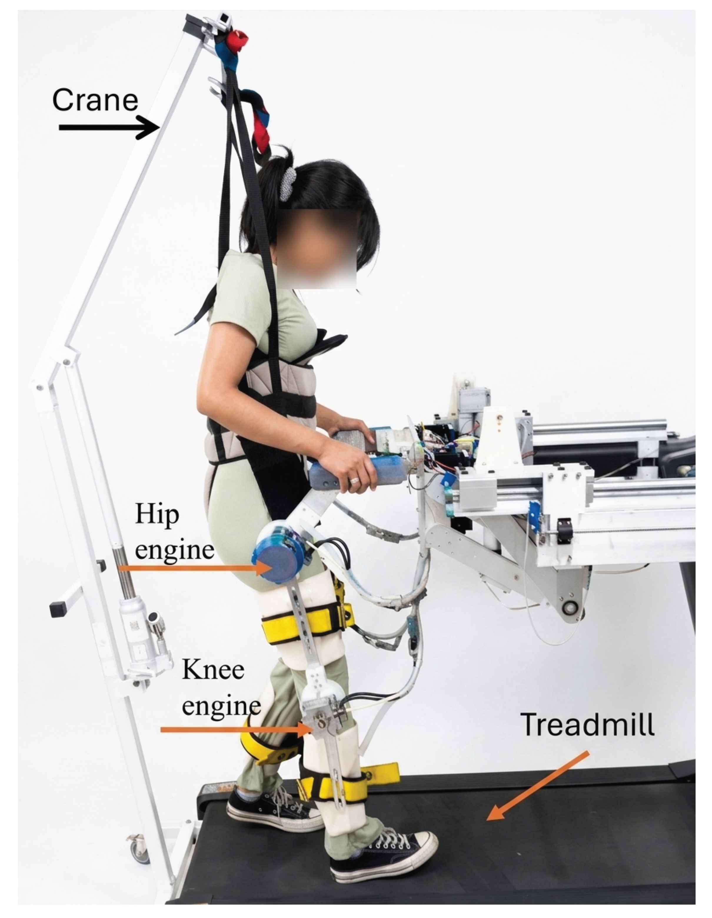
The exoskeleton used in this work was developed by the SANAS postgraduate program at CINVESTAV-IPN (Mexico City, Mexico) [29]. This exoskeleton has five degrees of freedom (DOFs): four for the lower limbs (two for the hips and two for the knees) and one for the sitting mechanism. It is important to note that all four joints (hips and knees) are rotationally elastic, featuring harmonic drive motors [30] with springs. An interesting characteristic of these actuators is their elastic damping during the gait cycle, which helps to create a more natural and comfortable walking experience for the user. For each joint, we can measure both the angular position of the link ( q e ) and the angular position of the motor ( q m ). Figure 1 shows the final prototype and the general distribution of its actuators. The prototype is split into two main sections: the elevation section and the lower-limb section. The elevation section includes a parallel mechanism and a safety harness connected to a crane, used to lift the subject. The lower-limb section consists of an exoskeleton that supports the legs, with the actuator axes aligning with the joints’ rotational axes. To simulate walking more accurately and provide a natural and comfortable feeling, the treadmill is synchronized with the exoskeleton, replicating movement and walking speed. Table 2 shows the dynamic parameters of the exoskeleton, as well as joint range of motion (ROM) and motor rated torque ( τ r ).
Figure 1. Experimental setup and prototype distribution.
Electronics 15 03992 g001
Table 2. Parameters of the physical exoskeleton prototype used in both numerical and experimental validations.
ParameterValueParameterValue
m 1 1.509 [kg] I 2 0.0116 [ kg · m 2 ]
m 2 1.500 [kg]Jdiag (0.01, 0.01) [ kg · m 2 ]
l c 1 0.0983 [m]Bdiag (0.015, 0.015) [N·m·s/rad]
l c 2 0.0229 [m]Kdiag (138.65, 138.65) [N·m/rad]
l 1 0.364 [m]ROM Hip−1/4 to π /2 [rad]
l 2 0.26 [m]ROM Knee0 to 2 [rad]
I 1 0.1213 [ kg · m 2 ] τ r 50 [Nm]
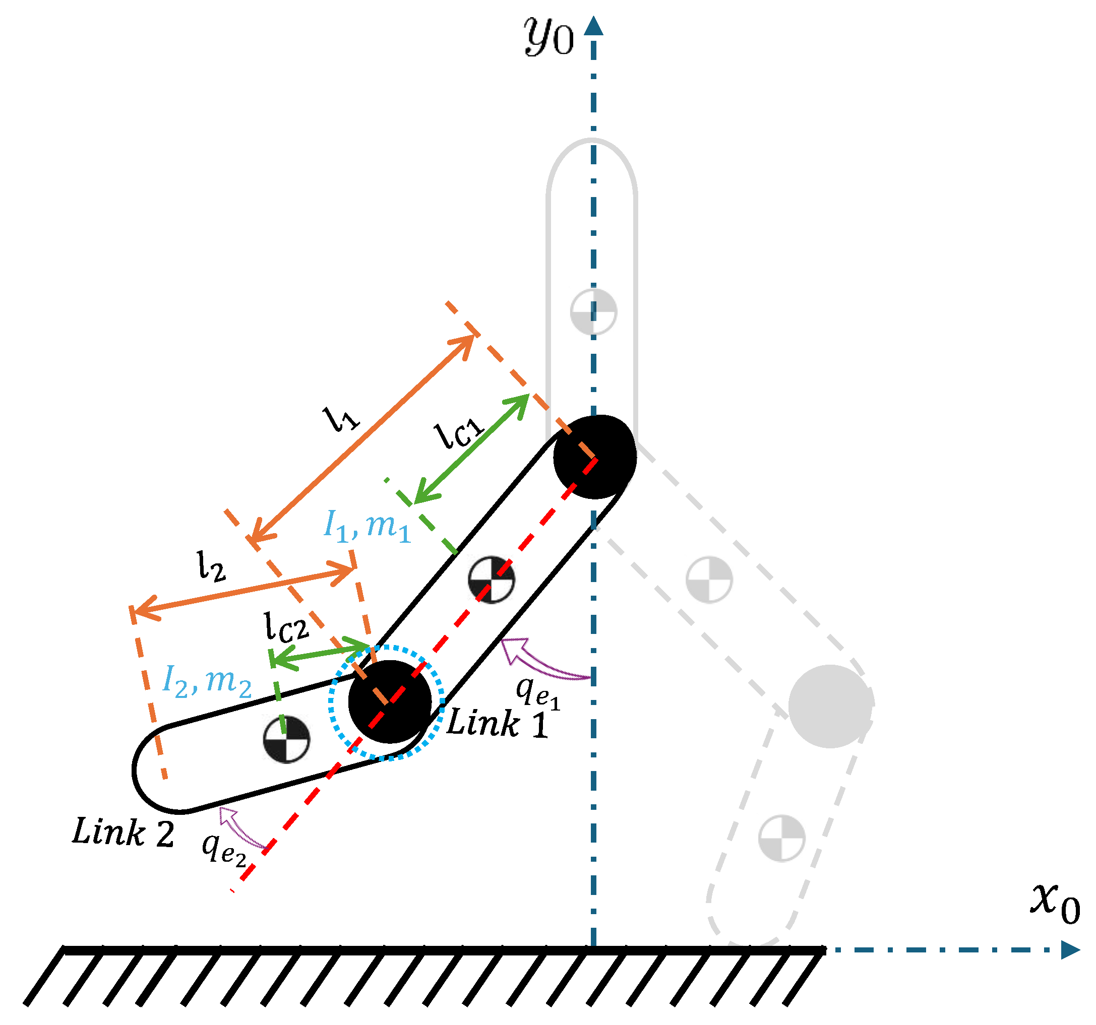
Note: m 1 , m 2 : link masses; l c 1 , l c 2 : center of mass positions; l 1 , l 2 : link lengths; I 1 , I 2 : link moments of inertia; J: motor inertia matrix; B: viscous damping matrix; K: joint stiffness matrix; ROM: range of motion; τ r : rated actuator torque. See Figure 2.
Figure 2. Schematic diagram of the exoskeleton’s leg with elastic joints.
Electronics 15 03992 g002

2.2. Anthropometric Characteristics of the Exoskeleton User

The experimental tests were conducted with a healthy 22-year-old female participant, weighing 52 kg with a height of 1.64 m. Before starting the trials, the participant was informed about the exoskeleton’s safety systems, specifically the mechanical stops that limit the range of motion to prevent hyperextension of the lower limbs and the electrical emergency stop button that completely deactivates the system. Once informed, the participant signed an informed consent form detailing the aforementioned conditions.
The mass approximation of the main segments (thigh, shank, and foot) of the human lower limb (Table 3) was obtained using the anthropometric tables by De Leva (1996) [31].
The rationale for selecting a single healthy subject for this initial experimental phase was to strictly prioritize safety and establish a reliable baseline for the mechanical stability and control performance of the exoskeleton prototype before proceeding to clinical trials. A detailed analysis of this limitation is elaborated in the Discussion Section.

2.3. Mathematical Model of the Exoskeleton with Elastic Joints

Using the Euler–Lagrange formalism [32], the dynamical model of the exoskeleton’s leg with SEA can be expressed as
M ( q e ) q ¨ e + C ( q e , q ˙ e ) q ˙ e + g ( q e ) = K [ q m q e ] = τ SEA J q ¨ m + B q ˙ m + K [ q m q e ] = τ
where q m = [ q m 1 q m 2 ] T and q e = [ q e 1 q e 2 ] T are the angular positions of motors 1 and 2 and links 1 and 2, respectively. M R 2 × 2 is the inertia matrix of exoskeleton, C R 2 × 2 is the Coriolis matrix of exoskeleton, g R 2 is the vector of gravitational forces of exoskeleton and K is the positive definite diagonal matrix with the stiffness coefficient of elastic element on the diagonal defined as: K = d i a g { k 1 , k 2 } . J is a positive definite diagonal matrix with values in its diagonal equal to the product of the inertia moments of the rotors and the square of the gear ratio: J = d i a g { J 1 r 1 , 1 2 , J 2 r 1 , 2 2 } . B is a positive definite diagonal matrix, and its values are the viscous friction parameters of each motor B = d i a g { b 1 , b 2 } . τ R 2 is the input torques of the actuators.
The dynamic elements of the symmetric inertia matrix M ( q e ) = [ m i j ] , the Coriolis and centrifugal matrix C ( q e , q ˙ e ) = [ c i j ] , and the gravitational vector g ( q e ) = [ g 1 , g 2 ] T are defined as
m 11 = I 1 + I 2 + m 1 l c 1 2 + m 2 ( l 1 2 + l c 2 2 + 2 l 1 l c 2 cos ( q e 2 ) ) m 12 = m 21 = I 2 + m 2 ( l c 2 2 + l 1 l c 2 cos ( q e 2 ) ) m 22 = I 2 + m 2 l c 2 2
c 11 = m 2 l 1 l c 2 sin ( q e 2 ) q ˙ e 2 , c 12 = m 2 l 1 l c 2 sin ( q e 2 ) ( q ˙ e 1 + q ˙ e 2 ) c 21 = m 2 l 1 l c 2 sin ( q e 2 ) q ˙ e 1 , c 22 = 0
g 1 = ( m 1 l c 1 + m 2 l 1 ) g cos ( q e 1 ) + m 2 l c 2 g cos ( q e 1 + q e 2 ) g 2 = m 2 l c 2 g cos ( q e 1 + q e 2 )
where g = 9.81   m/s 2 .

2.4. Control Strategies

2.4.1. PD+G

Proportional–derivative control with gravity compensation (PD+G) is one of the most widely used classical control strategies for robot manipulators and other nonlinear systems given its simplicity and low computational cost. This control law is defined as
τ = K p e + K d e ˙ + g ( q e )
where K p and K d are positive definite gain matrices. The position or tracking error (depending on the control objective) is defined as e = q e des q e , where q e des is the desired position and q e is the actual position. The velocity error is defined as e ˙ = q ˙ e des q ˙ e , where q ˙ e des is the desired velocity and q ˙ e is the actual velocity. Finally, g ( q e ) corresponds to the vector of gravitational torques of the dynamic system.
Combining Equations (1) and (5) yields the closed-loop dynamics
M ( q e ) q ¨ e + C ( q e , q ˙ e ) q ˙ e + g ( q e ) = K p e + K d e ˙ + g ( q e ) .
A necessary and sufficient condition for the origin [ e T e ˙ T ] T = 0 R 2 n to be an equilibrium point of the closed-loop system is that the desired position satisfies the following expression:
M ( q e des ) q ¨ e des + C ( q e des , q ˙ e des ) q ˙ e des = 0
To prove the stability of the origin as an equilibrium point, the direct Lyapunov method is employed. Consider the following Lyapunov candidate function,
V ( e , q ˙ e ) = 1 2 q ˙ e T M ( q e ) q ˙ e + 1 2 e T K p e
whose time derivative is given by
V ˙ ( e , q ˙ e ) = q ˙ e T M ( q e ) q ¨ e + 1 2 q ˙ e T M ˙ ( q e ) q ˙ e + e T K p e ˙ .
Substituting M ( q e ) q ¨ e from the closed-loop equation and applying the skew-symmetry property of the matrix M ˙ ( q ) 2 C ( q , q ˙ ) , the expression simplifies to
V ˙ ( e , q ˙ e ) = q ˙ e T K d q ˙ e .
Therefore, V ˙ ( e , q ˙ e ) 0 , demonstrating that the system is stable in the sense of Lyapunov. To prove asymptotic stability when the damping matrix K d is positive semi-definite (as occurred in the optimization results where the knee joint damping gain was set to zero), LaSalle’s invariance principle is applied. Let Ω = { ( e , q ˙ e ) : V ˙ ( e , q ˙ e ) = 0 } . From (10), V ˙ = 0 implies that the hip velocity q ˙ e 1 = 0 . For the system to remain within this invariant set, its derivative must also vanish ( q ¨ e 1 = 0 ). Substituting these conditions into the closed-loop dynamics (6) yields a coupled algebraic relationship where the physical coupling matrix C ( q e , q ˙ e ) and the structural stiffness of the series elastic actuators (SEAs) force the unactuated or undamped internal dynamics to converge. Consequently, the largest invariant set contained in Ω is restricted to the origin [ e T e ˙ T ] T = 0 R 4 , guaranteeing local asymptotic stability.
One of the main advantages of the PD+G controller is its ease of implementation as it requires minimal computational resources and relies solely on the knowledge of the gravitational torque vector rather than the full nonlinear dynamic model. For set-point regulation tasks (where q ˙ e des = q ¨ e des = 0 ), this classical strategy successfully guarantees global asymptotic stability.
However, it is crucial to emphasize that the lower-limb rehabilitation protocol executed in this study requires continuous trajectory tracking, meaning q e des ( t ) is time-varying. Under such tracking conditions, the uncompensated velocity and acceleration reference terms ( M ( q e ) q ¨ e des + C ( q e , q ˙ e ) q ˙ e des ) act as non-vanishing perturbation inputs to the closed-loop error dynamics. Consequently, the origin is no longer an exact equilibrium point. Instead, the PD+G control law ensures uniform ultimate boundedness (UUB) ([33], Chapter 4), [34], meaning the tracking error e and velocity error e ˙ will not diverge but will remain bounded within a compact region around the origin. The radius of this bounded region depends heavily on the magnitude of the reference trajectory derivatives and the stiffness of the chosen gains. This theoretical limitation of classical non-model-based tracking inherently explains the larger phase lags and position tracking errors experimentally observed for the PD+G and PID algorithms when compared to fully compensated robust sliding mode architectures.
Despite its operational simplicity, minimizing this bounded tracking error depends entirely on the optimal tuning of the gain matrices K p and K d . While traditionally tuned heuristically or through empirical methods such as Ziegler–Nichols [35] and Harriott [36], these classical approaches are heavily discouraged in robotic applications due to the risk of inducing severe mechanical stress during the tuning phase. To overcome this limitation, bio-inspired optimization algorithms, such as genetic algorithms (GAs) [37] and particle swarm optimization (PSO) [38], are systematically employed. These offline tuning techniques evaluate the nonlinear model safely, minimizing tracking errors and finding the optimal bounds for K p and K d without exposing the physical actuators to unnecessary wear.

2.4.2. PID

Similar to the PD+G controller, proportional–integral–derivative (PID) control is a commonly used strategy for systems that are not overly complex. The control law is defined as
τ = K p e + K d e ˙ + K i 0 t e ( τ ) d τ
where K p , K i and K d are positive definite gain matrices. The position or tracking error (depending on the control objective) is defined as e = q e des q e , where q e des is the desired position and q e is the actual position. The proportional term K p e is responsible for reducing the instantaneous error, the derivative term K d e ˙ helps to reduce oscillations that may occur during the transient phase, and the integral term K i e ( τ ) d τ helps to reduce or eliminate the steady-state error. The velocity error is defined as e ˙ = q ˙ e des q ˙ e .
This control law can be expressed through the following two equations:
τ = K p e + K d e ˙ + k i ξ ξ ˙ = e
Consequently, the closed-loop dynamics are given by
M ( q e ) q ¨ e + C ( q e , q ˙ e ) q ˙ e + g ( q e ) = K p e + K d e ˙ + k i ξ
The equilibrium points of this equation take the form [ ξ T e T e ˙ T ] T and must be a constant vector for the origin to be considered an equilibrium point.
This equilibrium point can be shifted to the origin through the following change of variables:
z = ξ K i 1 g ( q e des )
For further stability analysis, the following global change of variables is proposed,
w e q ˙ e = α I I 0 0 I 0 0 0 I z e q ˙ e
with α > 0 .
To prove stability of the state space origin, the direct Lyapunov method is employed by proposing the following candidate function,
V ( e , q ˙ e , w ) = 1 2 w e q ˙ e T 1 α K i 0 0 0 α K d α M ( q e ) 0 α M ( q e ) M ( q e ) w e q ˙ e + 1 2 e T K p 1 α K i e + U ( q e des e ) U ( q e des ) + e T g ( q e des )
where U ( q e ) denotes the potential energy of the robot and α is the positive constant used in the change of variables. These variables are selected as detailed in [39].
Once the conditions are established, the function is globally positive definite. Thus, by applying the skew-symmetry property, its time derivative is expressed as
V ˙ ( e , q ˙ e , w ) = q ˙ e T [ K d α M ( q e ) ] q ˙ e e T [ α K p K i ] e α e T C ( q e , q ˙ e ) T q ˙ e α e T [ g ( q e des ) g ( q e ) ]
Following the considerations from [39], V ˙ is negative semi-definite, demonstrating that V ˙ 0 only within a ball D of radius η > 0 around the state space origin. Because V ˙ is only locally negative semi-definite, LaSalle’s invariance principle adapted for local regions is applied [39]. Evaluating the set where V ˙ = 0 strictly deduces that q ˙ e = 0 and e = 0 . Therefore, the origin of the closed-loop system is a locally asymptotically stable equilibrium point.
However, this type of control has limitations, just like with the PD+G controller; sometimes, it can be difficult to tune the K p , K i and K d gains. This controller is usually tuned heuristically or by using methods such as Ziegler–Nichols or Cohen–Coon. Poor tuning can cause instability or overshoot problems; the derivative action, if not implemented carefully, can cause the system to oscillate excessively and lead to instability in addition to amplifying noise from a sensor signal. Properly implementing it can result in good performance in systems that are not overly complex or highly nonlinear.
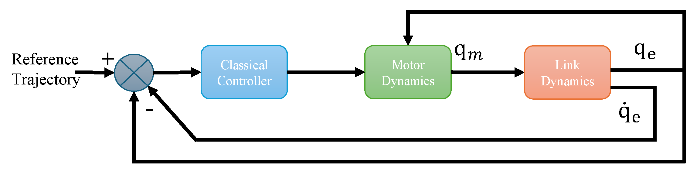
To illustrate the practical application of classical control strategies on the elastic-joint framework, Figure 3 depicts the detailed closed-loop block diagram. In this implementation, the classical feedback action operates directly upon the link tracking error e = q e d e s q e . The resulting control torque τ drives the motor dynamics, which naturally couples with the rigid link parameters via the physical spring deformation framework.

2.4.3. Computed Torque Sliding Mode Control (CT-SMC)

Sliding mode control (SMC) is a robust control strategy. This strategy is suitable for robot manipulators due to its ability to reject external disturbances, parametric uncertainties, and nonlinearities in the system. This control consists of designing a sliding surface where, once reached, the system dynamics becomes robust or insensitive to certain variations in the dynamic model. However, one of the main problems with traditional SMC is “chattering”, which is caused by the use of a discontinuous control signal. This phenomenon can cause faster wear on the plant’s actuators, as well as vibrations within them. This problem has been addressed in various ways, including the use of super-twisting sliding mode control (Section 2.4.4). The development of the computed torque SMC is presented below:
From the first equation in (1),
M ( q e ) q ¨ e + C ( q e , q ˙ e ) q ˙ e + g ( q e ) = K [ q m q e ] = τ SEA ,
considering the torque transmitted by the elastic element as the effective control input to the robot [40], u = τ SEA . The position and velocity errors are defined as
q ˜ e = q e q e des q ˜ ˙ e = q ˙ e q ˙ e des ,
and the sliding surface [41,42] as
s = q ˜ ˙ e + Λ q ˜ e ,
where Λ = Λ T > 0 . Differentiating with respect to time yields
s ˙ = q ¨ e q ¨ e des + Λ q ˜ ˙ e s ˙ = M 1 u C ( q e , q ˙ e ) q ˙ e g ( q e ) q ¨ e des + Λ q ˜ ˙ e .
The following control law is proposed [43],
u d = M q ¨ e des Λ q ˜ ˙ e k s a t ( s / ϕ ) + C ( q e , q ˙ e ) q ˙ e + g ( q e ) ,
with k > 0 and
s a t ( / ϕ ) = 1 > ϕ ϕ | | ϕ 1 < ϕ
where ϕ > 0 and being small.
Substituting (21) into (20) leads to
s ˙ = k s a t ( s / ϕ ) ) .
To guarantee stability, the following Lyapunov candidate function is proposed,
V = 1 2 s 2 ,
and its time derivative is given by
V ˙ = s T s ˙ = k s T s a t ( s / ϕ ) 0 ,
According to Lyapunov stability theory, s 0 ; as long as s = q ˜ ˙ e + Λ q ˜ e , then q ˜ e 0
This control action computes the desired torque u d = τ SEA des , but the actuator does not apply this torque directly to the links. Instead, the torque is generated through the spring deflection τ SEA = K [ q m q e ] . Consequently,
q m des = K 1 u d + q e .
This virtual reference q m des , derived from the robust computed torque SMC controller, serves as the reference to the second equation from (1) (the actuator dynamics), which the motor can track through a simple controller
τ = J q ¨ m des K v q ˜ ˙ m K p q ˜ m + B q ˙ m + K [ q m q e ]
where
q ˜ m = q m q m des

2.4.4. Computed Torque–Super-Twisting Sliding Mode Control (CT–ST-SMC)

Similar to the previous controller, starting from the first equation in (1),
M ( q e ) q ¨ e + C ( q e , q ˙ e ) q ˙ e + g ( q e ) = K [ q m q e ] = u ,
where u = τ SEA is the torque transmitted by the elastic element. The position and velocity errors are defined identically to the previous section,
q ˜ e = q e q e des q ˜ ˙ e = q ˙ e q ˙ e des ,
as well as the sliding surface and its time derivative,
s = q ˜ ˙ e + Λ q ˜ e s ˙ = q ¨ e q ¨ e des + Λ q ˜ ˙ e s ˙ = M 1 u C ( q e , q ˙ e ) q ˙ e g ( q e q ¨ e des + Λ q ˜ ˙ e .
with Λ = Λ T > 0 . However, the control law proposed for this case is
u = M q ¨ e des Λ q ˜ ˙ e + v + C ( q e , q ˙ e ) q ˙ e + g ( q e ) ,
Choosing
v = k 1 | s | 1 / 2 s g n ( s ) + z z ˙ = k 2 s g n ( s ) ,
with k 1 , k 2 > 0 , we obtain
s ˙ = k 1 | s | 1 / 2 s g n ( s ) + z z ˙ = k 2 s g n ( s ) .
The above equations correspond to the standard super-twisting algorithm (STA) introduced by Levant [44]. According to the finite-time convergence theorem for second-order sliding mode [45], if k 1 , k 2 are selected to satisfy the STA design conditions, then the equilibrium ( s , z ) = ( 0 , 0 ) is globally finite-time stable. Consequently, s 0 and s ˙ 0 in finite time.
Since s = q ˜ ˙ e + Λ q ˜ e and Λ is a positive definite matrix, the reduced-order dynamics satisfy q ˜ ˙ e + Λ q ˜ e = 0 , which implies q ˜ e 0 . Therefore, the tracking error converges asymptotically to zero.

2.4.5. Backstepping–Super-Twisting Sliding Mode Control (BS–ST-SMC)

In order to implement a backstepping controller, it is considered that the dynamics of the robot links is cascaded with the dynamics of the robot motors [46]. The dynamics of the links are driven by the motor angles q m through the flexible joints, while the dynamics of the motors are driven by the motor torques τ . Rearranging the dynamical model of the System (1), we have
M ( q e ) q ¨ e + C ( q e , q ˙ e ) q ˙ e + g ( q e ) + K q e = K q m q ¨ m = J 1 ( τ K ( q m q e ) B q ˙ m )
Considering q m as the input of the first equation in (34), a control law q m des R 2 for q m is proposed as
q m des = q e + K 1 [ M ( q e ) v ˙ + C ( q e , q ˙ e ) v + g ( q e ) K d r ]
where K d > 0 R 2 × 2 is diagonal and constant,
V = q ˙ e des Λ q ˜ e , q ˜ e = q e q e des , r = q ˙ e V ,
and V , q ˜ e and r R 2 , Λ > 0 R 2 × 2 is diagonal and constant.
Defining q ˜ m = q m q m des R 2 and substituting in the first equation of (34), we have
M ( q e ) r ˙ + C ( q e , q ˙ e ) r + K d r = K q ˜ m
Lyapunov’s function candidate is chosen as
V 1 = 1 2 r T M ( q e ) r
The time derivative along the trajectories of the system is
V ˙ 1 = 1 2 r T M ˙ ( q e ) r + r T M ( q e ) r ˙ = r T K d r + r T K q ˜ m
If q ˜ m = 0 , then V ˙ 1 < 0 and r tends to zero when t 0 and as r = q ˜ ˙ e + Λ q ˜ e , so q ˜ ˙ e and q ˜ e tend to zero when t .
In a second stage, q m is deemed as the input of the second equation of (34). Deriving q ˜ m as q ˜ ˙ m = q ˙ m q ˙ m des and q ˜ ¨ m = q ¨ m q ¨ m des and substituting into (34) yields
q ˜ ¨ m = J 1 ( τ B q ˙ m + K ( q e q m ) ) q ¨ m des
Now, defining the sliding surface as
s = q ˜ ˙ m + q ˜ m ,
and its derivative
s ˙ = q ˜ ¨ m + q ˜ ˙ m = J 1 ( τ B q ˙ m + K ( q e q m ) ) q ¨ m des + q ˜ ˙ m ,
the control law is proposed based on the continuous nonsingular terminal sliding mode algorithm framework [47], which embeds the fractional power within the integral term to enhance convergence,
τ = B q ˙ m K ( q e q m ) + J q ¨ m des J q ˜ ˙ m J K 1 | s | 1 / 2 s g n ( s ) + K 2 0 t | s | 1 / 2 s g n ( s ) d τ
where s g n ( · ) is a sign function. K 1 and K 2 are positive definite diagonal matrices.
So, when substituting it into (42), we have
s ˙ = K 1 | s | 1 / 2 s g n ( s ) + K 2 0 t | s | 1 / 2 s g n ( s ) d τ
and we can express s ˙ like
s ˙ 1 = K 1 | s 1 | 1 / 2 s g n ( s 1 ) + s 2
s ˙ 2 = K 2 | s 1 | 1 / 2 s g n ( s 1 )
A Lyapunov’s function candidate is chosen as
V = 1 2 s 2 2 + 0 s 1 K 2 | p | 1 / 2 s g n ( p ) d p 0
with derivative as
V ˙ = s 2 s ˙ 2 + K 2 | s 1 | 1 / 2 s g n ( s 1 ) s ˙ 1
Substituting (45) and (46) in the previous equation we obtain that
V ˙ = s 2 K 2 | s 1 | 1 / 2 s g n ( s 1 ) + K 1 | s 1 | 1 / 2 s g n ( s 1 ) s 2 K 2 | s 1 | 1 / 2 s g n ( s 1 ) ,
and then
V ˙ = K 1 K 2 | s 1 | 0
By LaSalle theorem s 1 0 , from (46) s 2 0 s 0 , and, if s 0 , then q ˜ ˙ m 0 , q ˜ 0 and q ˜ ¨ m 0 .
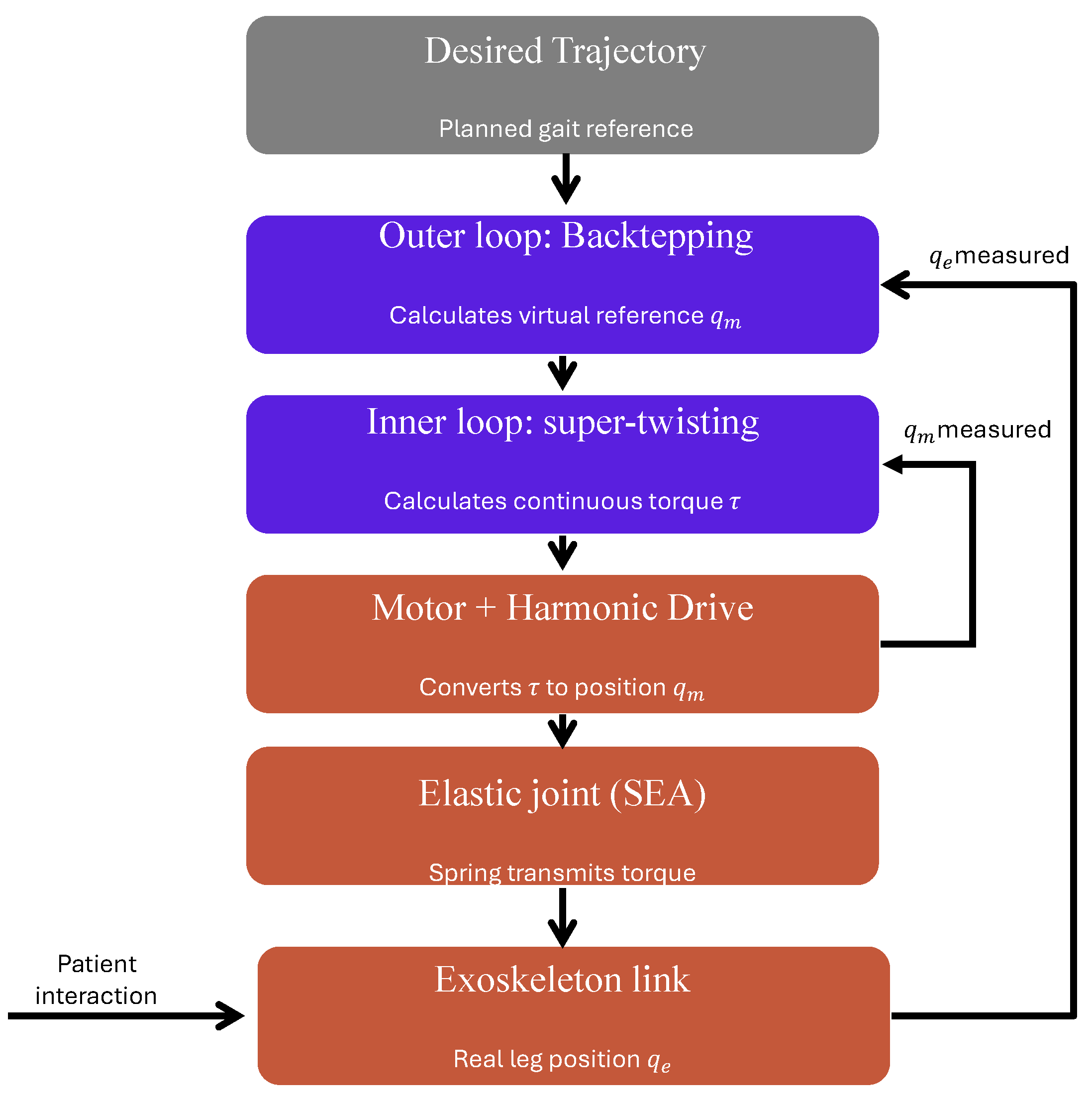
To illustrate the practical execution of the proposed control law, the comprehensive algorithmic sequence within the real-time loop is mapped out sequentially. Figure 4 delineates the detailed operational workflow of the hybrid BS–ST-SMC architecture, illustrating the deterministic steps from the physical sensor feedback acquisition ( q e , q ˙ e , q m , q ˙ m ) to the multi-stage computational blocks that ultimately transmit the command torque τ to the actuators.

3. Experimental and Numerical Results

3.1. Numerical Results

The numerical validation of the dynamic model was carried out in the MATLAB R2026a® Simulink R2026a environment using the inertial parameters shown in Table 2 and Table 3. To establish a fair and unbiased benchmark across all the control schemes—effectively isolating their structural capabilities from heuristic tuning discrepancies—a unified multi-objective particle swarm optimization (PSO) algorithm was employed. This framework systematically optimizes the gains of each controller to minimize tracking errors while simultaneously preserving biological motion smoothness and preventing actuator torque saturation. The explicit objective function J evaluated for each particle is defined as
J = W 1 · MSE p + W 2 · MSE v + W 3 · J I + W 4 · P τ
where MSE p and MSE v denote the mean squared errors of position and velocity, respectively. The jerk index ( J I ) [ rad 2 / s 5 ], which quantifies motion smoothness, is computed as the integral of the squared joint jerk over the execution cycle T,
J I = 0 T d 3 q e ( t ) d t 3 2 d t ,
and P τ = max ( 0 , | τ | τ limit ) is a soft-constraint penalty function heavily penalizing torques exceeding the actuator limit of 50 Nm. The position error, velocity error, and jerk components were min–max normalized to [ 0 , 1 ] using historical empirical bounds prior to evaluation. This allowed the assignment of equal objective weights ( W 1 = W 2 = W 3 = 1.0 ), while the saturation penalty was strictly enforced with a heavy multiplier ( W 4 = 10 4 ).
For each controller, 150 particles and 50 iterations per cycle were executed over four cycles. To search for the optimal gain vector X i (e.g., X i = [ K p , K i , K d ] T for PID), the swarm dynamics evolve by updating the velocity ( V i ) and position ( X i ) profiles at each iteration k, (53) V i k + 1 = w V i k + c 1 r 1 ( P b e s t , i X i k ) + c 2 r 2 ( G b e s t X i k ) (54) X i k + 1 = X i k + V i k + 1 where c 1 = c 2 = 2.0 are the cognitive and social acceleration coefficients, and r 1 , r 2 U ( 0 , 1 ) introduce stochastic behavior. The vector P b e s t , i denotes the historical personal best position of the i-th particle, while G b e s t represents the global optimum discovered by the entire swarm. To ensure stable convergence, the initial search space [ 0 5000 ] was reduced by 60 % in subsequent cycles, the inertia weight w decayed dynamically from 0.9 to 0.45, and a velocity clipping boundary restricted the maximum step size to 10 % of the search bounds.
The pseudo-random number generator was initialized with a fixed seed of 42 to guarantee deterministic reproducibility. Furthermore, the PSO algorithm was independently executed 10 times to evaluate stochastic variance. The standard deviation of the final optimal cost across all 10 independent runs was less than 1.0 % , confirming robust convergence to the global optimum. The best-performing particle from these executions provided the optimal gains presented in Table 4.
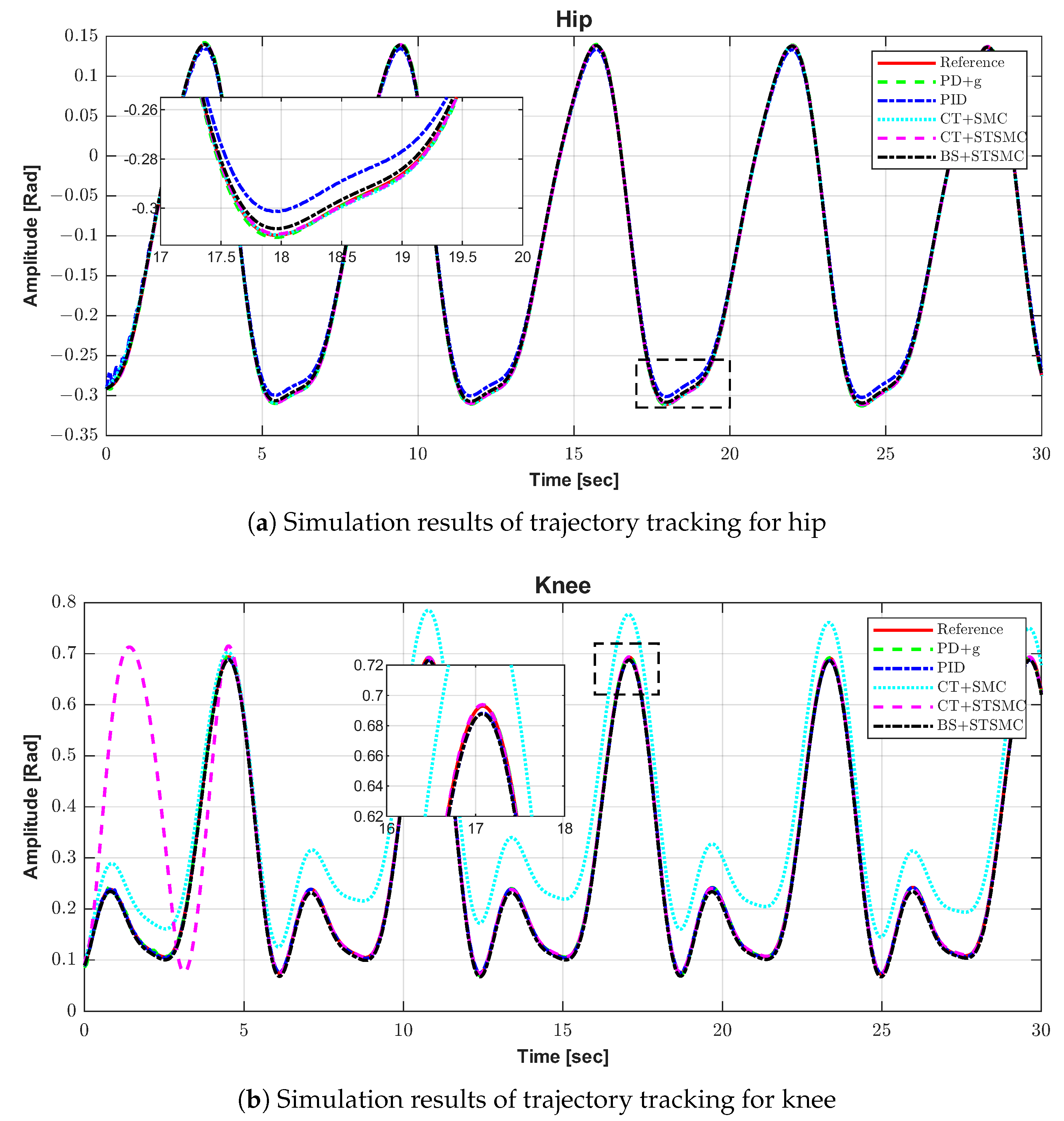
Performance metrics obtained with these optimal gains under ideal conditions—that is, assuming that the dynamic parameters of the exoskeleton and the patient are perfectly known and assuming the absence of external disturbances—are presented in Table 5.
Figure 5 illustrates the trajectory tracking performance of the hip and knee links for each proposed controller, assuming ideal conditions as presented in Table 5.
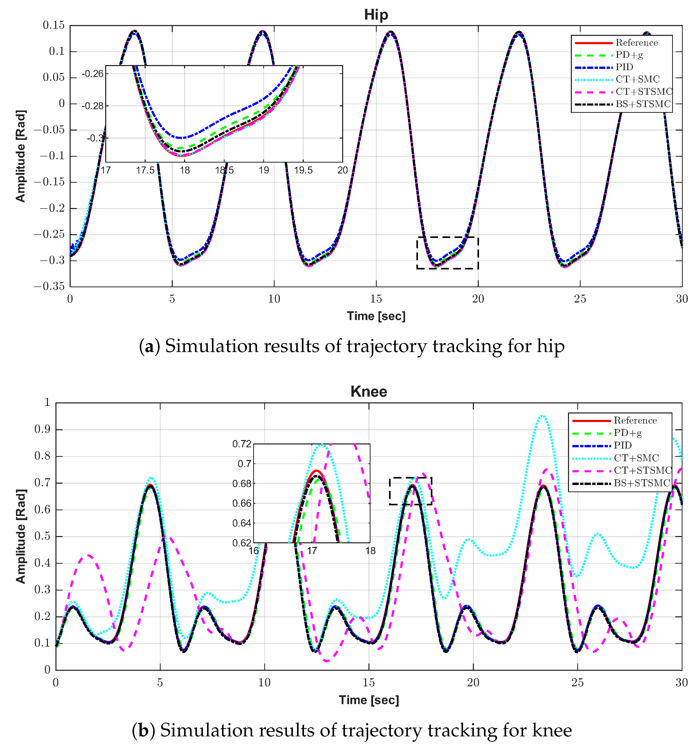
However, to bring this comparison closer to reality, a second numerical evaluation was performed. The optimal gains found with the PSO algorithm were retained, but this time parametric uncertainties and external disturbances were introduced. Specifically, we consider the realistic scenario where the mass contribution of each body segment cannot be perfectly known, and the patient slightly resists the movement (either due to muscle stiffness or residual force). To simulate these conditions, the patient’s mass was increased by 20% in the dynamic model (but not in the controllers) and an opposing force directly proportional to the movement of each link was added (which can be interpreted as a viscous friction acting on the links). The performance metrics obtained under these conditions are presented in Table 6, while Figure 6 shows the tracking graphs under these same conditions.

3.2. Experimental Results

The real-time control algorithms and sensor data acquisition were executed on an NI myRIO-1900 embedded device running LabVIEW at a sampling frequency of 21 Hz. The rehabilitation gait trajectory was obtained from predefined biomechanical routines reported in Ref. [28], designed to replicate natural lower-limb motion. During all the experimental trials, the treadmill speed was strictly maintained at 0.25 km/h, which represents the clinical baseline speed recommended for early-stage lower-limb gait retraining. Each evaluation consisted of three continuous walking trials per controller to verify steady-state behavior.
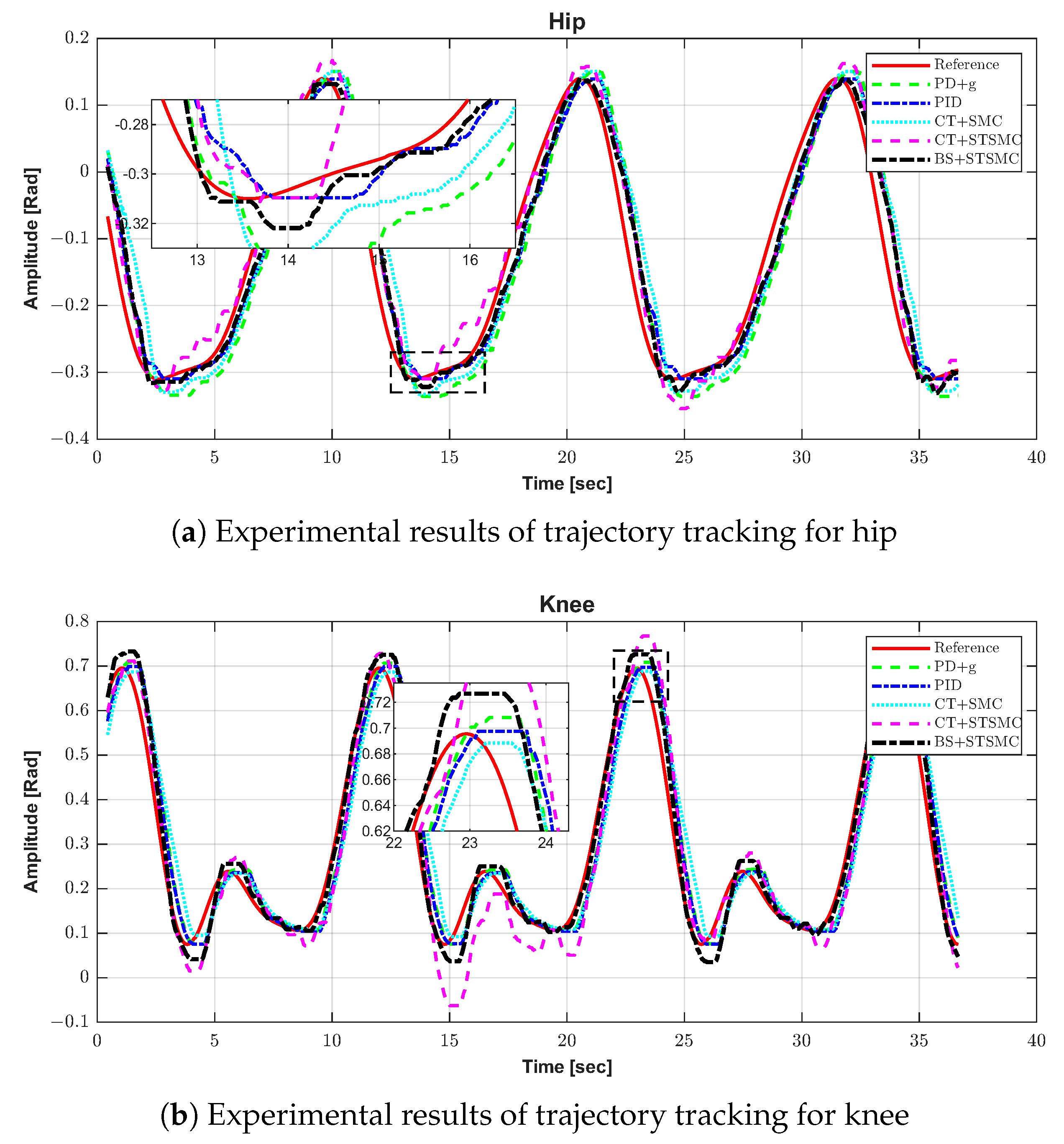
All the experimental tests were conducted under identical conditions using the exoskeleton prototype described in Section 2.1 and the test subject described in Section 2.2. The performance metrics obtained from these trials for each of the presented controllers are shown in Table 7. Similarly, Figure 7 illustrates the trajectory tracking performance obtained from the experimental tests.
To ensure statistical repeatability and assess the consistency of the controllers, a protocol of three full walking trials was executed for each control strategy. During data post-processing, negligible variance was observed across the consecutive trials due to the controlled laboratory environment and treadmill synchronization. Therefore, the data presented in Table 7 and Figure 7 correspond to the third and final trials of each controller, capturing the fully developed steady-state gait cycle.

4. Discussion

The experimental and numerical validation of the five control strategies implemented on the CINVESTAV lower-limb rehabilitation exoskeleton reveals critical performance trade-offs. These insights are essential for understanding how classical, model-based robust, and cascaded architectures handle highly nonlinear coupled human–robot dynamics within a rotationally elastic joint configuration.

4.1. Tracking Accuracy and Robustness Under Parametric Uncertainties

When analyzing the position tracking accuracy across the ideal simulation (Table 5), non-ideal simulation (Table 6), and physical human trials (Table 7), a distinct shift in performance occurs. Under ideal conditions, the model-dependent architectures, such as computed torque–super-twisting sliding mode control (CT–ST-SMC), achieve an exceptionally low mean squared position error (MSEp) for the hip link ( 3.13 × 10 8 rad ). However, when subjected to non-ideal dynamic conditions—simulating a 20 % patient mass mismatch and human muscle resistance friction—classical architectures experience significant degradation. For instance, the knee link MSEp for the proportional–derivative with gravity compensation (PD+G) controller increases by more than two orders of magnitude, jumping from 2.23 × 10 6 rad to 3.22 × 10 4 rad .
In contrast, the proposed hybrid backstepping–super-twisting sliding mode controller (BS–ST-SMC) demonstrates superior tracking stability across environments. In the physical experimental trials (Table 7), the BS–ST-SMC consistently yields the lowest tracking errors, securing an MSEp of 1.32 × 10 3 rad at the hip and 2.32 × 10 3 rad at the knee. While a portion of this improved tracking authority is naturally enabled by the higher gain margins discovered during the PSO optimization, this superior performance also strongly reflects the theoretical capability of the proposed cascaded architecture. The backstepping core effectively pre-compensates for the link dynamics by generating an explicit virtual motor trajectory ( q m d e s ), while the super-twisting outer loop enforces a continuous sliding mode that handles both unmodeled human-in-the-loop interactions and varying link compliance without losing tracking authority.

4.2. Chattering Suppression and Biomechanical Smoothness

A core objective in gait neurorehabilitation is providing a natural, smooth, and safe user experience that is directly quantified by the jerk index. Traditional sliding mode control (CT-SMC) is notorious for high-frequency control chattering. This issue is highlighted in the numerical results (Table 5 and Table 6), where the knee joint under CT-SMC exhibits a massive jerk index ( 1.44 × 10 7 and 8.70 × 10 7 , respectively), accompanied by high-power consumption. Such structural vibrations cause premature wear on the series elastic actuators (SEAs) and present a safety risk to the patient.
The application of the second-order sliding mode algorithm via the super-twisting approach drastically mitigates this issue. By embedding the high-frequency switching element within an integral term, the actual torque commands τ become continuous. Experimentally (Table 7), the BS–ST-SMC restricts the jerk index to 5.67 × 10 4 at the hip and 8.33 × 10 4 at the knee. These smoothness levels are closely comparable to the PID baseline ( 4.11 × 10 4 and 8.28 × 10 4 ). This balance proves that the hybrid controller provides robust tracking without introducing the high-frequency control torque spikes that are common in basic sliding mode control applications.
It is important to note the numerical scaling discrepancy of the jerk index between the idealized numerical simulations and the physical experiments. In simulation (Table 5 and Table 6), the absence of sensor noise and the mathematical perfection of the tracking profiles result in extremely low J I magnitudes (< 10 6 rad 2 / s 5 ). However, during physical experimental trials (Table 7), the high-frequency measurement noise from the sensors, combined with voluntary muscular adjustments and tremor from the human participant, naturally amplify the third derivative of the position. This shifts the operational experimental J I into the 10 4 to 10 5 rad 2 / s 5 range, which remains within safe and comfortable physical interaction limits for rehabilitation robotics.

4.3. Phase Lag and Joint Actuator Coherence

The interaction between the harmonic drive motor position ( q m ) and the elastic link position ( q e ) creates a flexible dynamic coupling that introduces an inherent phase lag. Minimizing this phase lag is crucial for human–exoskeleton coordination. During physical implementation (Table 7), the classical PID controller suffers from an extensive phase lag at the hip (14.54°) and knee (11.13°). This lag occurs because decoupled linear feedback cannot adapt to rapid changes in human limb dynamics during the gait cycle. The BS–ST-SMC successfully addresses this lag by utilizing its cascaded design. By calculating a virtual reference trajectory for the motor q m d e s within the backstepping loop and applying the super-twisting sliding surface to the motor error vector q ˜ m , the phase delay is minimized. This configuration achieves an experimental phase lag of only 4.22° at the knee joint. Reduced phase lag ensures that the exoskeleton actively guides the user through the nominal trajectory instead of dragging behind the lower limbs, which matches the clinical goals of passive training therapies.
In order to bound the control problem under measurable and adversarial operational conditions, the physical validation inherently subjected the architectures to the non-ideal scenarios requested by numerical benchmarks. Parameter uncertainty was induced by a 20 % variation in the nominal human-limb mass parameters during tracking cycles. Furthermore, high-frequency sensor noise was natively injected into the loops through the raw encoder differentiation required to compute q ˙ e and the jerk index ( J I ). The experimental results in Section 4 demonstrate that, while classical PID performance degraded under these unmodeled dynamics and noise amplification, the robust BS–ST-SMC restricted the tracking boundaries efficiently, preserving stability without control signal saturation.

4.4. Discrepancies Between Simulation and Experimental Trials

A notable aspect of the study is the change in metrics from numerical simulation to experimental conditions. In the ideal simulation, peak torques frequently reach the saturation boundary of 50 Nm for robust controllers. However, in physical experiments, the maximum values remain beneath 10.02 Nm across all the architectures.
This difference occurs because the simulated trajectories demand instantaneous acceleration changes that the real physical system tempers through structural damping, spring compliance, and internal sensor filtering. Furthermore, the physical participant introduces a level of compliance and soft tissue damping that acts as a natural low-pass filter on control actions. This behavior confirms that, while the PSO algorithm effectively searches the parameter space using the numeric model, the built-in flexibility of the SEA prototype offers a crucial safety buffer during real-world execution.
These discrepancies between ideal dynamics and physical hardware also explain the behavior of the optimal gains found by the PSO algorithm (Table 4). The algorithm actively pushed the robust sliding mode gains to high values (e.g., k 1 reaching 6760.7276 for the BS–ST-SMC) to forcefully reject the continuous torque disturbances introduced by the rotationally elastic spring coupling. Conversely, the zero derivative gain ( K d , 22 = 0 ) obtained for the knee joint in the PD+G and PID controllers is physically justified: the intrinsic elasticity (K) and structural viscous damping (B) of the knee’s series elastic actuator already provide significant passive dissipation. Introducing an active derivative control action would over-damp the joint, unnecessarily increasing the tracking phase lag.

4.5. Study Limitations

Despite the promising tracking and chattering-suppression results demonstrated by the BS–ST-SMC, this study presents certain limitations. The experimental validation was conducted as a proof-of-concept pilot study involving a single healthy subject. While this approach safely establishes the baseline performance and robustness of the control architectures under physical human–robot interaction, it does not fully capture the complex pathological gait dynamics, muscle spasticity, or varying degrees of motor impairment that are present in actual stroke or spinal cord injury patients. Furthermore, while the BS–ST-SMC exhibited superior overall performance in position tracking and phase lag reduction, classical controllers like PID showed competitive behavior in peak torque minimization under specific conditions, indicating that the ultimate control selection must be tailored to the specific therapeutic goals.
Another methodological aspect to consider is the inherent coupling between controller architecture and parameter optimization. Although all the control strategies were tuned under an identical multi-objective PSO framework with uniform performance criteria to ensure a fair evaluation, advanced robust controllers naturally feature higher parametric flexibility. This expanded search space facilitates superior disturbance rejection compared to fixed-structure linear baselines, meaning that the observed experimental performance reflects both the architectural decoupling of the flexible dynamics and the efficacy of the nonlinear gain optimization.

5. Conclusions

This paper presents a detailed experimental evaluation of five control strategies applied to a lower-limb rehabilitation exoskeleton featuring series elastic actuators. To ensure an objective comparison, a multi-objective particle swarm optimization (PSO) algorithm was used to optimize the controller gains based on MSEp, MSEv, and jerk index criteria.
The experimental results validate the following core conclusions:
  • Classical approaches like PID and PD+G offer low computational overhead and smooth profiles, but they suffer from significant phase lag (>11°) and degraded accuracy when subjected to human interaction forces.
  • While traditional computed torque SMC improves trajectory tracking, it introduces significant chattering and structural stress, as shown by its high jerk index.
  • The hybrid backstepping–super-twisting sliding mode controller (BS–ST-SMC) demonstrates highly balanced and effective overall performance, particularly in tracking accuracy and motion smoothness. While it achieves the lowest experimental position error ( 1.32 × 10 3 rad 2 MSEp) and minimizes knee phase lag to just 4.22°, it is important to note that classical controllers like PID remain highly competitive—and occasionally superior—in minimizing peak torque and power consumption under specific steady-state conditions. This indicates that the ultimate control selection must be tailored to the specific therapeutic goals of the rehabilitation session.
These findings confirm that cascaded nonlinear architectures are highly suitable for elastic-joint wearable systems. However, as this research currently serves as a proof of concept, our application-oriented roadmap for future work includes expanding the subject sample size and recruiting patient populations with lower-limb motor impairments to formally validate its clinical value. Additionally, future research will explore active rehabilitation control modes driven by human intention detection and the integration of intelligent radial basis function (RBF) neural networks into the backstepping loop to adaptively estimate varying patient dynamics without manual recalibration.


Author Contributions

Conceptualization, Y.R.-L. and S.J.R.-P.; methodology, Y.R.-L.; software, Y.R.-L., S.J.R.-P. and Y.C.-G.; validation, Y.R.-L., S.J.R.-P. and Y.C.-G.; formal analysis, Y.R.-L. and S.S.; investigation, S.J.R.-P. and Y.C.-G.; resources, S.S. and R.L.; data curation, Y.R.-L.; writing—original draft preparation, Y.R.-L., S.J.R.-P. and Y.C.-G.; writing—review and editing, S.S. and R.L.; visualization, S.J.R.-P. and Y.C.-G.; supervision, S.S. and R.L.; project administration, Y.R.-L., S.S. and R.L.; funding acquisition, S.S. and R.L. All authors have read and agreed to the published version of the manuscript.

Funding

This research received no external funding.

Institutional Review Board Statement

The study was conducted in accordance with the Declaration of Helsinki and the protocol was approved by the Ethics and Safety Committee for Research in Human Beings of the National Laboratory in Autonomous Vehicles and Exoskeletons of the Center for Research and Advanced Studies of the National Polytechnic Institute, CDMX, México.

Informed Consent Statement

All subjects gave their informed consent for inclusion before they participated in the study.

Data Availability Statement

The original contributions presented in this study are included in the article. Further inquiries can be directed to the corresponding author.

Conflicts of Interest

The authors declare no conflicts of interest.

References

  1. Organización Mundial de la Salud. Informe mundial la discapacidad. Educación 2011, 218, 219. [Google Scholar]
  2. Cuenot, M. Clasificación Internacional del Funcionamiento, de la Discapacidad y de la Salud. EMC Kinesiterapia Med. Fís. 2018, 39, 1–6. [Google Scholar] [CrossRef] [Scilit]
  3. García, C.E.; Sánchez, A.S. Clasificaciones de la OMS sobre discapacidad. Boletín RPD 2001, 50, 15–30. [Google Scholar]
  4. Gam, L.T.H.; Quan, D.H.; Ngoc, P.V.B.; Quan, B.H.; Thanh, B.T. Position–Force Control of a Lower-Limb Rehabilitation Robot Using a Force Feed-Forward and Compensative Gravity Proportional Derivative Method. Electronics 2024, 13, 4494. [Google Scholar] [CrossRef] [Scilit]
  5. De Sire, A.; Invernizzi, M. Musculoskeletal rehabilitation: State-of-the-art. Appl. Sci. 2021, 11, 6243. [Google Scholar] [CrossRef] [Scilit]
  6. Wyss, J. Therapeutic Programs for Musculoskeletal Disorders; Demos Medical Publishing: New York, NY, USA, 2012. [Google Scholar]
  7. Barnes, M. Principles of neurological rehabilitation. J. Neurol. Neurosurg. Psychiatry 2003, 74, iv3–iv7. [Google Scholar] [CrossRef] [Scilit]
  8. Mashud, G.; Hasan, S.; Alam, N. Advances in Control Techniques for Rehabilitation Exoskeleton Robots: A Systematic Review. Actuators 2025, 14, 108. [Google Scholar] [CrossRef] [Scilit]
  9. Hasan, S.; Alam, N. Comprehensive Comparative Analysis of Lower Limb Exoskeleton Research: Control, Design, and Application. Actuators 2025, 14, 342. [Google Scholar] [CrossRef] [Scilit]
  10. Firouzi, V.; Seyfarth, A.; Song, S.; von Stryk, O.; Ahmad Sharbafi, M. Biomechanical models in the lower-limb exoskeletons development: A review. J. Neuroeng. Rehabil. 2025, 22, 12. [Google Scholar] [CrossRef] [Scilit]
  11. Marinou, G.; Kourouma, I.; Mombaur, K. Development and validation of a modular sensor-based system for gait analysis and control in lower-limb exoskeletons. Sensors 2025, 25, 2379. [Google Scholar] [CrossRef] [Scilit]
  12. Sarajchi, M.; Sirlantzis, K. Design and control of a single-leg exoskeleton with gravity compensation for children with unilateral cerebral palsy. Sensors 2023, 23, 6103. [Google Scholar] [CrossRef] [Scilit]
  13. Shakeriaski, F.; Mohammadian, M. Enhancing Upper Limb Exoskeletons Using Sensor-Based Deep Learning Torque Prediction and PID Control. Sensors 2025, 25, 3528. [Google Scholar] [CrossRef] [Scilit]
  14. Rahmatillah, A.; Adinda, A.; Hanifah, U.; Fadilah, M.H.; Rulaningtyas, R.; Septanto, H. Control system design for lower limb robotic exoskeleton using fuzzy-tuned PID. AIP Conf. Proc. 2025, 3346, 020006. [Google Scholar]
  15. Rosales-Luengas, Y.; Salazar, S.; Rangel-Popoca, S.J.; Cortés-García, Y.; Flores, J.; Lozano, R. Active Gait Retraining with Lower Limb Exoskeleton Based on Robust Force Control. Appl. Sci. 2025, 15, 4032. [Google Scholar] [CrossRef] [Scilit]
  16. Wong Sang, M.; Narayan, J. Reinforcement Learning-Based Finite-Time Sliding-Mode Control in a Human-in-the-Loop Framework for Pediatric Gait Exoskeleton. Machines 2025, 13, 668. [Google Scholar] [CrossRef] [Scilit]
  17. Zhang, G.; Gong, F.; Wang, J.; Wang, Y.; Zhang, L. Prescribed performance sliding mode control for wearable exoskeletons with constrained states. Appl. Math. Model. 2025, 144, 116027. [Google Scholar] [CrossRef] [Scilit]
  18. Narayan, J.; Dwivedy, S.K. Pediatric gait training using a lower-limb exoskeleton with adaptive finite-time sliding mode control scheme: An experimental study. Trans. Inst. Meas. Control. 2025, 47, 1438–1454. [Google Scholar] [CrossRef] [Scilit]
  19. Aly, A.A.; Vu, M.T.; El-Sousy, F.F.; Hsia, K.H.; Alotaibi, A.; Mousa, G.; Le, D.N.; Mobayen, S. Adaptive Neural Network-Based Fixed-Time Tracking Controller for Disabilities Exoskeleton Wheelchair Robotic System. Mathematics 2022, 10, 3853. [Google Scholar] [CrossRef] [Scilit]
  20. Aly, A.A.; Hsia, K.H.; El-Sousy, F.F.; Mobayen, S.; Alotaibi, A.; Mousa, G.; Le, D.N. Adaptive neural backstepping control approach for tracker design of wheelchair upper-limb exoskeleton robot system. Mathematics 2022, 10, 4198. [Google Scholar] [CrossRef] [Scilit]
  21. Yang, Y.; Huang, D.; Ma, L.; Liu, X.; Li, Y. Adaptive neural fault-tolerant prescribed performance control of a rehabilitation exoskeleton for lower limb passive training. ISA Trans. 2024, 151, 143–152. [Google Scholar] [CrossRef] [Scilit]
  22. Li, J.; Wang, Q.; Fang, Y. Adaptive neural network-based practical predefined-time nonsingular terminal sliding mode control for upper limb rehabilitation robots. Commun. Nonlinear Sci. Numer. Simul. 2024, 136, 108085. [Google Scholar] [CrossRef] [Scilit]
  23. Fang, Y.; Zhang, J.; Li, Y. Neural networks adaptive predefined-time control for pure-feedback nonlinear systems: A case study on robotic exoskeleton systems. Sci. Rep. 2025, 15, 6041. [Google Scholar] [CrossRef] [Scilit]
  24. Baud, R.; Manzoori, A.R.; Ijspeert, A.; Bouri, M. Review of control strategies for lower-limb exoskeletons to assist gait. J. Neuroeng. Rehabil. 2021, 18, 119. [Google Scholar] [CrossRef] [Scilit]
  25. Wang, X.; Zhang, C.; Yu, Z.; Deng, C. Decoding of lower limb continuous movement intention from multi-channel sEMG and design of adaptive exoskeleton controller. Biomed. Signal Process. Control. 2024, 94, 106245. [Google Scholar] [CrossRef] [Scilit]
  26. Narayan, J.; Abbas, M.; Dwivedy, S.K. Adaptive backstepping sliding mode subject-cooperative control for a pediatric lower-limb exoskeleton robot. Trans. Inst. Meas. Control. 2025, 47, 352–368. [Google Scholar] [CrossRef] [Scilit]
  27. Li, J.; Jiang, H.; Gao, M.; Li, S.; Wang, Z.; Pang, Z.; Zhang, Y.; Jiao, Y. Research on Iterative Learning Method for Lower Limb Exoskeleton Rehabilitation Robot Based on RBF Neural Network. Appl. Sci. 2025, 15, 6053. [Google Scholar] [CrossRef] [Scilit]
  28. Yuan, T.; Zhang, C.; Yi, F.; Lv, P.; Zhang, M.; Li, S. RBFNN-Based Adaptive Integral Sliding Mode Feedback and Feedforward Control for a Lower Limb Exoskeleton Robot. Electronics 2024, 13, 1043. [Google Scholar] [CrossRef] [Scilit]
  29. CINVESTAV—Sistemas Autónomos de Navegación Aérea y Submarina. SANAS—CINVESTAV. 2025. Available online: https://www.cinvestav.mx/academia/posgrados/doctroado-sistemas-autonomos-de-navegacion-aerea-y-submarina (accessed on 17 July 2025).
  30. Pan, C.T.; Lee, M.C.; Huang, J.S.; Chang, C.C.; Hoe, Z.Y.; Li, K.M. Active assistive design and multiaxis self-tuning control of a novel lower limb rehabilitation exoskeleton. Machines 2022, 10, 318. [Google Scholar] [CrossRef] [Scilit]
  31. De Leva, P. Adjustments to Zatsiorsky-Seluyanov’s segment inertia parameters. J. Biomech. 1996, 29, 1223–1230. [Google Scholar] [CrossRef] [Scilit]
  32. Spong, M. Modeling and control of elastic joint robots. Math. Comput. Model. 1989, 12, 912. [Google Scholar]
  33. Lewis, F.L.; Dawson, D.M.; Abdallah, C.T. Robot Manipulator Control: Theory and Practice; CRC Press: Boca Raton, FL, USA, 2003. [Google Scholar]
  34. Dawson, D.M. Uncertainties in the Control of Robot Manipulators; Georgia Institute of Technology: Atlanta, GA, USA, 1990. [Google Scholar]
  35. Ziegler, J.G.; Nichols, N.B. Optimum settings for automatic controllers. Trans. ASME 1942, 64, 759–768. [Google Scholar] [CrossRef] [Scilit]
  36. Harriott, P. Process Control; McGraw-Hill: New York, NY, USA, 1964. [Google Scholar]
  37. Goldberg, D.E. Genetic Algorithms in Search, Optimization, and Machine Learning; Addison-Wesley: Reading, MA, USA, 1989. [Google Scholar]
  38. Kennedy, J.; Eberhart, R. Particle swarm optimization. In Proceedings of the ICNN’95-International Conference on Neural Networks, Perth, WA, Australia, 27 November–1 December 1995; Volume 4, pp. 1942–1948. [Google Scholar]
  39. Kelly, R.; Santibánes, V. Control de Movimiento de Robots Manipuladores; Pearson Educación-Prentice Hall: Mexico City, México, 2003. [Google Scholar]
  40. Siciliano, B.; Sciavicco, L.; Villani, L.; Oriolo, G. Robotics: Modelling, Planning and Control; Springer: Berlin/Heidelberg, Germany, 2009. [Google Scholar]
  41. Utkin, V.I. Sliding Modes in Control and Optimization; Springer Science & Business Media: Berlin/Heidelberg, Germany, 2013. [Google Scholar]
  42. Slotine, J.J.E.; Li, W. Applied Nonlinear Control; Prentice Hall: Englewood Cliffs, NJ, USA, 1991; Volume 199. [Google Scholar]
  43. Spong, M.W. Robot Modeling and Control; John Wiley & Sons: Hoboken, NJ, USA, 2012. [Google Scholar]
  44. Levant, A. Higher-order sliding modes, differentiation and output-feedback control. Int. J. Control. 2003, 76, 924–941. [Google Scholar] [CrossRef] [Scilit]
  45. Moreno, J.A.; Osorio, M. Strict Lyapunov functions for the super-twisting algorithm. IEEE Trans. Autom. Control. 2012, 57, 1035–1040. [Google Scholar] [CrossRef] [Scilit]
  46. Sciavicco, L.; Siciliano, B. Modelling and Control of Robot Manipulators; Springer Science & Business Media: Berlin/Heidelberg, Germany, 2012. [Google Scholar]
  47. Fridman, L.; Moreno, J.A.; Bandyopadhyay, B.; Kamal, S.; Chalanga, A. Continuous nested algorithms: The fifth generation of sliding mode controllers. In Recent Advances in Sliding Modes: From Control to Intelligent Mechatronics; Springer: Berlin/Heidelberg, Germany, 2015; pp. 5–35. [Google Scholar]
Figure 3. Control block diagram showcasing the closed-loop implementation of classical architectures (PID and PD+G) interacting with the series elastic actuator dynamics.
Electronics 15 03992 g003
Figure 4. Detailed execution workflow of the proposed hybrid BS–ST-SMC algorithm implemented within the real-time control loop.
Electronics 15 03992 g004
Figure 5. Simulation results of trajectory tracking for the hip (a) and knee (b) under ideal conditions (fully known parameters and no external disturbances).
Electronics 15 03992 g005
Figure 6. Simulation results of trajectory tracking for the hip (a) and knee (b) under realistic conditions (parameter uncertainties and external disturbances).
Electronics 15 03992 g006
Figure 7. Experimenta results of trajectory tracking for the hip (a) and knee (b) in the presence of parameter uncertainties and external disturbances.
Electronics 15 03992 g007
Table 1. Qualitative comparison of recent lower-limb exoskeleton control studies versus the proposed work.
StudyActuator TypeControl StrategiesSubjectsDisturbance TypeReported MetricsReal-Time Application
Sarajchi [12]Rigid actuatorPD+G/PID1 (pediatric)NonePosition errorYes
Narayan [18]Rigid actuatorAdaptive finite-time SMC1 (pediatric)Parametric variationsPosition error/jerkYes
Yang [21]Rigid actuatorAdaptive neural fault-tolerantSimulationFault injections/loadTracking errorNo (simulation only)
Yuan [28]Rigid actuatorRBFNN adaptive ISMCSimulationInteraction forcesPosition errorNo (simulation only)
This studySeries elastic actuator (SEA)PID/PD+G/CT-SMC/CT–ST-SMC/BS–ST-SMC1 (adult)Mass mismatch (+20%) & friction resistanceMSEp, MSEv, jerk, torque, power, and phase lagYes (experimental validations)
Table 3. Inertial parameters of the lower-limb segments.
ParameterValue
Thigh mass8.13 [kg]
Shank mass2.65 [kg]
Foot mass0.71 [kg]
Table 4. Optimal controller gains found using the PSO algorithm.
ControllerGainValue
PD+G K p diag([209.4915, 8.9701])
K d diag([0.8808, 0.0000])
PID K p diag([786.6276, 108.6608])
K i diag([0.4697, 0.5899])
K d diag([1.1838, 0.0000])
Computed torque SMCkdiag([25.7830, 93.0843])
Λ diag([142.5254, 763.8570])
K p diag([784.6372, 394.4882])
K v diag([2507.4494, 940.2417])
Computed torque–ST-SMC k 1 diag([0.6265, 3.4022])
k 2 diag([73.6570, 34.0304])
Λ diag([1303.8952, 26.0235])
K p diag([2058.8544, 395.4433])
K v diag([1943.3713, 920.5933])
Backstepping–ST-SMC k d diag([366.5169, 3.1301])
Λ diag([96.5126, 233.2897])
k 1 diag([6760.7276, 1742.5786])
k 2 diag([308.4699, 3.8740])
Table 5. Performance metrics obtained with ideal conditions.
Controller MSEpos [ rad 2 ] MSEvel [ ( rad / s ) 2 ] Peak Error [rad]Jerk Index [ rad 2 / s 5 ] Peak Torque [Nm]Peak Power [W]Phase Lag [°]
PD+GHip 1.09 × 10 6 1.80 × 10 6 0.0034 9.08 × 10 5 8.1618 1.4077 0.4065
Knee 2.23 × 10 6 7.33 × 10 6 0.0102 9.02 × 10 6 0.5840 0.3026 0.0581
PIDHip 3.89 × 10 5 1.10 × 10 3 0.0185 1.85 × 10 5 14.5509 2.6818 0.2903
Knee 7.59 × 10 6 1.00 × 10 3 0.0069 2.27 × 10 6 0.7464 0.3071 0.6387
ComputedHip 2.12 × 10 6 1.21 × 10 5 0.0095 4.80 × 10 4 50 9.3983 0.0
torque SMCKnee 6.80 × 10 3 3.95 × 10 4 0.1177 1.44 × 10 7 50 13.5365 1.1032
ComputedHip 3.13 × 10 8 2.73 × 10 6 0.0013 9.37 × 10 4 50 9.5290 0.0581
torque–ST-SMCKnee 1.33 × 10 2 2.12 × 10 2 0.5507 6.98 × 10 6 50 8.0455 0
BacksteppingHip 4.53 × 10 6 4.17 × 10 6 0.0035 5.20 × 10 4 50 17.3270 0.2930
–ST-SMCKnee 3.68 × 10 5 3.79 × 10 6 0.0064 1.16 × 10 7 50 11.2931 0.0
Table 6. Performance metrics obtained with non-ideal conditions and external perturbations.
Controller MSEpos [ rad 2 ]MSEvel [(rad/s)2]Peak Error [rad]Jerk Index [rad2/s5]Peak Torque [Nm]Peak Power [W]Phase Lag [°]
PD+GHip 8.90 × 10 6 1.13 × 10 4 0.0082 5.88 × 10 5 9.1905 1.5749 0.5226
Knee 3.22 × 10 4 1.33 × 10 4 0.0343 3.09 × 10 6 0.8397 0.4114 3.3677
PIDHip 5.04 × 10 5 9.48 × 10 4 0.0207 3.82 × 10 4 16.2607 3.2269 0.2323
Knee 1.43 × 10 5 2.73 × 10 4 0.0080 2.02 × 10 5 0.8787 0.4226 0.5226
ComputedHip 9.38 × 10 6 3.58 × 10 5 0.0184 2.35 × 10 5 50 17.5976 0.0
torque SMCKnee 3.10 × 10 2 3.32 × 10 3 0.3346 8.70 × 10 7 50 31.1259 5.3419
ComputedHip 5.90 × 10 8 4.16 × 10 6 0.0016 5.73 × 10 4 50 9.5798 0.0
torque–ST-SMCKnee 2.42 × 10 2 6.51 × 10 2 0.4065 7.04 × 10 6 50 7.8415 26.0710
BacksteppingHip 4.32 × 10 6 4.25 × 10 6 0.0034 7.90 × 10 4 50 17.3124 0.2323
–ST-SMCKnee 3.78 × 10 5 3.70 × 10 6 0.0070 1.09 × 10 7 50 9.6033 0.0581
Table 7. Performance metrics obtained from experimental tests.
Controller MSEpos [rad2]MSEvel [(rad/s)2]Peak Error [rad]Jerk Index [rad2/s5]Peak Torque [Nm]Peak Power [W]Phase Lag [°]
PD+GHip 2.91 × 10 3 3.66 × 10 3 0.1112 6.89 × 10 4 7.0670 2.0776 19.481
Knee 3.30 × 10 3 7.01 × 10 3 0.1186 8.24 × 10 4 7.4355 3.1317 9.2200
PIDHip 1.75 × 10 3 2.62 × 10 3 0.0970 4.11 × 10 4 6.6905 1.8995 14.546
Knee 4.47 × 10 3 8.80 × 10 3 0.1537 8.28 × 10 4 7.6693 4.1070 11.133
ComputedHip 3.39 × 10 3 4.75 × 10 3 0.1457 7.96 × 10 4 5.4582 1.6843 14.395
torque SMCKnee 5.72 × 10 3 8.64 × 10 3 0.1645 3.90 × 10 4 6.5686 2.3847 11.813
ComputedHip 1.40 × 10 3 4.96 × 10 3 0.0962 5.99 × 10 4 6.9187 2.3810 3.8252
torque–ST-SMCKnee 4.36 × 10 3 1.17 × 10 2 0.1956 1.03 × 10 5 10.014 5.4918 9.0123
BacksteppingHip 1.32 × 10 3 3.27 × 10 3 0.1016 5.67 × 10 4 5.7179 2.0275 12.380
–ST-SMCKnee 2.32 × 10 3 8.45 × 10 3 0.1141 8.33 × 10 4 9.4190 5.3162 4.2242
Disclaimer/Publisher’s Note: The statements, opinions and data contained in all publications are solely those of the individual author(s) and contributor(s) and not of MDPI and/or the editor(s). MDPI and/or the editor(s) disclaim responsibility for any injury to people or property resulting from any ideas, methods, instructions or products referred to in the content.