Zero-LUT Open-Set Plankton Classification on Edge MPSoC and GPU Platforms

Abstract

Autonomous plankton monitoring needs classifiers that run on low-power edge hardware and reject out-of-distribution (OOD) inputs. Our prior in situ plankton image biomass estimation (IsPlanktonBIO) framework identifies organisms by nearest-neighbour search over a similarity gallery, a memory-resident lookup that stalls 8-bit integer (INT8) acceleration and grows with the corpus. We replace it with a zero look-up-table (Zero-LUT) linear energy head: a matrix-multiply-only scorer over a supervised-contrastive backbone that needs no database and shrinks the footprint sevenfold, to 1.3 MB. We assess recognition and rejection jointly with an open-set protocol based on the correct-classification rate at a fixed OOD-leakage budget, showing that closed-set accuracy alone misleads. Our hardware–software co-design on an AMD Kria KV260 Multiprocessor System-on-Chip (MPSoC) runs the INT8 pipeline in real time at 86.5% end-to-end accuracy; its calibrated gate accepts 82.9% of in-distribution images, rejects 89.0% of OOD inputs, and correctly labels 97.6% of those accepted. INT8 conversion raises two issues: classification varies for background-dominated patterns, and OOD thresholds must be recalibrated on the compressed model, not inherited from full precision. An NVIDIA Jetson Orin Nano Super port reproduces this behaviour: the GPU is faster and more energy-efficient, whereas the MPSoC’s reconfigurable logic can host sensing and control beside the accelerator.

1. Introduction

Planktonic organisms form the base of marine food webs and drive the biological carbon pump. Traditionally, biological oceanography relied on direct sample collection, but the field has shifted toward non-invasive in situ observation using optical imaging instruments. Devices such as the Imaging Plankton Probe (IPP) [1] have produced massive datasets like DYB-PlanktonNet [2], enabling deep learning (DL) models for automated taxonomic classification [3,4]. However, most systems today follow a “Cloud Intelligence” paradigm: instruments transmit raw data to remote servers for processing, introducing significant latency and bandwidth costs. To address these bottlenecks, recent research has shifted computation toward “Edge Intelligence,” where devices perform inference directly on-device for real-time decision-making [5]; shipboard systems already run plankton classifiers on edge hardware at sea for adaptive, real-time sampling [6,7].

1.1. Problem Statement

This on-device shift for plankton monitoring, however, exposes a critical trade-off between computational demand and energy availability. Recent software frameworks build on an image-retrieval paradigm: IsPlanktonIR [8] trains a supervised-contrastive feature extractor and identifies query images by nearest-neighbour similarity to a reference gallery, and our own prior work, IsPlanktonBIO [9], extends this scheme to joint taxonomic classification and biomass estimation, scoring each detection against a cosine-similarity look-up table (LUT). Both frameworks were developed and validated on workstation Graphics Processing Units (GPUs); their deployment on autonomous platforms is constrained by hardware limitations, and, as we show, the retrieval LUT itself becomes a bottleneck on edge devices. Figure 1 compares the IsPlanktonBIO baseline framework with our proposed zero look-up-table (Zero-LUT) alternative. The scoring step is the co-design bottleneck, whether used for classification, as in the IsPlanktonBIO baseline framework (Figure 1a); or repurposed for out-of-distribution rejection, as in this work (Figure 1b). Briefly, the IsPlanktonBIO baseline scores each detection with a FAISS (Facebook AI Similarity Search, v1.9.0) cosine-similarity search over a memory-resident embedding index (look-up table, LUT): the index occupies approximately 8 MB of ARM Processing System (PS) RAM at run time (≈233 MB to build), and its nearest-neighbour search runs on the ARM cores in the interval between the two DPU (Deep-Learning Processor Unit) calls, stalling the 8-bit integer (INT8) accelerator. The proposed Zero-LUT Linear Energy (LE) scorer replaces the search with a LogSumExp over the classifier logits that reduces to a single general matrix multiply (GEMM), whose only parameters are the 1.3 MB fully-connected weights already compiled into the model. Removing the resident index shrinks the scorer footprint roughly sevenfold and keeps the DPU fed. Underwater vehicles, gliders, and profiling buoys operate under strict energy budgets that often preclude the use of high-performance GPUs typically used for training these models. Furthermore, computationally intensive deep learning inference often requires remote servers, introducing latency that hinders real-time monitoring. Therefore, optimising these algorithms for resource-constrained embedded systems without compromising scientific rigor remains an open engineering challenge.

1.2. Contribution

To close this gap, we adapt our own workstation-GPU IsPlanktonBIO pipeline [9] to the Edge Intelligence paradigm. We replace its nearest-neighbour scorer with a matrix-multiply-only Zero-LUT energy head and assemble an open-set evaluation protocol (Section 3.4) that let a plankton classifier reject such unfamiliar, out-of-distribution images while still running reliably once compressed for low-power hardware. We validate this through a hardware–software co-design on an AMD Kria KV260 Multiprocessor System-on-Chip (MPSoC; Advanced Micro Devices, Inc., Santa Clara, CA, USA). The methodology itself is platform-agnostic: porting the pipeline to an NVIDIA Jetson Orin Nano Super (NVIDIA Corporation, Santa Clara, CA, USA) reproduces the same accuracy and rejection behaviour, and we report openly where that embedded GPU is the more efficient inference target. The main contributions of this work are:

• A Zero-LUT Linear Energy out-of-distribution (OOD) scorer: a LogSumExp head over a supervised-contrastive (SupCon) backbone whose only heavy operation is a general matrix multiply (GEMM). It replaces the memory-resident FAISS nearest-neighbour search, removing both the embedding index that stalls the DPU and the cold-start gallery whose build cost grows with the training corpus, and cutting the runtime scorer footprint roughly sevenfold, to 1.3 MB, with no database dependency. We adopt it as a deployability decision, not a claim of OOD superiority: the FAISS scorers separate OOD inputs more accurately, but only the energy head meets the platform’s zero-external-memory, DPU-only constraint.
• An empirical study, to our knowledge among the first, of how a post hoc out-of-distribution scorer behaves once the classifier is compressed to INT8 for a two-stage edge accelerator. It surfaces two deployment findings, confirmed on both edge platforms: a host-side INT8 preprocessing rounding quirk that can silently break classification on background-dominated crops and generalises to any toolchain where the host produces the fixed-point tensor, and the need to recalibrate OOD rejection thresholds on the compressed model rather than inherit them from full precision.
• A bottleneck analysis of the multi-stage pipeline on the Kria KV260: replacing the FAISS scorer with the Zero-LUT engine and then enabling two-image pipelining lift sustained throughput from 19.6 to 38.0 FPS at 300 MHz, reaching 89.8% DPU utilisation (Section 4.2.3).
• Power and energy-per-image measurements across four hardware-aware compression strategies (iterative and one-step coarse-grained pruning, Once-For-All, and Fast Neural Architecture Search), quantifying their impact on accuracy, OOD robustness, and the energy budget of autonomous platforms.

1.3. Organisation of the Paper

The remainder of this paper is organised as follows. Section 2 reviews the closest edge instruments, Field-Programmable Gate Array (FPGA)/MPSoC accelerators and out-of-distribution methods. Section 3 describes the two-stage architecture and its partition into the Processing System (PS) and the Programmable Logic (PL) on the Kria KV260, the dataset and OOD partitioning, the training and INT8 quantisation procedure, the open-set evaluation protocol, and the backbone and OOD-scorer selection. Section 4 reports the 32-bit floating-point (FP32) algorithmic performance and then the deployed INT8 pipeline on the Kria KV260, closing with the head-to-head comparison against an NVIDIA Jetson Orin Nano Super. Section 5 discusses the trade-offs, transferable lessons and limitations, and Section 6 draws the major conclusions and future work.

2. Related Work

Focused on the design of a plankton imaging solution, this paper primarily addresses two challenges: the hardware platform deployment; and the processing of out-of-distribution (OOD) samples. Both design decisions are largely independent of each other. As neither problem is specific to plankton imaging, we review three adjacent literatures in turn: the edge and in situ instruments that motivate an on-device plankton classifier in the first place (Section 2.1), the FPGA and MPSoC accelerators that supply a candidate platform for it (Section 2.2), and the out-of-distribution and open-set recognition methods that supply its rejection stage (Section 2.3).

2.1. Edge and In-Situ Instruments for Plankton Imaging

Automated plankton observation is moving from bench-top flow cytometers toward autonomous instruments that image and classify organisms directly in the water column. Recent systems bring inference close to the sensor: shipboard classifiers already run at sea to steer adaptive sampling [6,7], low-cost flow-imaging devices have been paired with machine-learning pipelines for real-time algal-bloom monitoring [10], and compact submersible holographic microscopes perform passive microbial sensing at depth [11]. On the recognition side, the image-retrieval lineage of IsPlanktonIR [8] and IsPlanktonBIO [9] reaches high accuracy but identifies each organism by nearest-neighbour matching against a reference gallery, a design developed and validated on workstation GPUs. However, neither framework pairs this recognition capability with an edge-deployable out-of-distribution rejection mechanism. IsPlanktonIR already tests a rejection threshold for unfamiliar organisms, but only atop the same memory-resident gallery LUT. IsPlanktonBIO, the pipeline this work adapts, has not yet implemented such rejection at all, listing it explicitly as future work. Neither system, moreover, has been evaluated under the INT8, memory- and latency-constrained regime that on-device deployment demands. Our study targets what these lines rarely combine: an out-of-distribution-aware plankton classifier that runs entirely on low-power edge hardware, without the memory-resident gallery the retrieval paradigm presumes.

2.2. FPGA and MPSoC Accelerators for Embedded Vision

When transferring vision-based models to embedded devices, selecting the computing platform is critical. While Application-Specific Integrated Circuits (ASICs) offer maximum efficiency, their lack of flexibility and long time-to-market [12] make them less suitable for rapidly evolving research platforms. Table 1, synthesised from [13], summarises these trade-offs across five figures of merit. Field-Programmable Gate Arrays (FPGAs) are a robust alternative whose reconfigurable fabric can integrate custom sensor interfacing and deterministic control alongside the deep-learning accelerator on a single device, and have been reported energy-competitive with embedded GPUs in some configurations [14,15]. Modern System-on-Module (SOM) architectures, such as the AMD Xilinx Kria series, integrate a Multiprocessor System-on-Chip (MPSoC) that combines ARM processors with programmable logic, where ARM cores handle deterministic computer vision tasks while the FPGA fabric accelerates deep learning inference through a dedicated Deep-Learning Processor Unit (DPU) overlay and its associated toolchain [16].

This heterogeneous architecture is a well-established route to real-time convolutional inference under strict power budgets: concrete deployments include underwater image recognition on an FPGA embedded system [17], convolutional backbones mapped to the Vitis-AI DPU on a multi-engine FPGA SoC [18], deep character recognition on a Zynq UltraScale+ MPSoC [19], and on-board hyperspectral classification accelerators for small satellites [20]. Nearest to our platform, a sibling study from the same MPSoC family instantiates a two-DPU iris detection-and-segmentation pipeline on a Zynq UltraScale+ device and, as we also observe, reports the accelerator saturating on-chip UltraRAM (URAM) within a sub-10 W envelope [21], exposing the same programmable-logic ceiling we analyse in Section 4.2.7. These works confirm that FPGA and MPSoC targets meet embedded real-time and power constraints. Elsewhere, Schlessman et al. [22] justify their FPGA choice over a conventional multi-core PC on cost, power and footprint grounds for discreet outdoor deployment, regardless of the PC’s raw computational ability. None, however, couples the accelerated backbone with an out-of-distribution rejection stage, nor examines how INT8 quantisation perturbs that rejection decision, which is the gap this work addresses.

Table 1. Qualitative platform trade-offs for Deep Neural Network (DNN) inference acceleration, synthesised from [13]. +  = high; o = medium; − = low.

Figure of Merit	GPU	FPGA	ASIC
Peak throughput	+	o	+
Energy efficiency	o	o	+
Reconfigurability	+	+	–
Development time-to-market	+	o	–
Unit cost (high volume)	o	o	+

Table 1. Qualitative platform trade-offs for Deep Neural Network (DNN) inference acceleration, synthesised from [13]. +  = high; o = medium; − = low.

Figure of Merit	GPU	FPGA	ASIC
Peak throughput	+	o	+
Energy efficiency	o	o	+
Reconfigurability	+	+	–
Development time-to-market	+	o	–
Unit cost (high volume)	o	o	+

2.3. Out-of-Distribution and Open-Set Recognition

Rejecting inputs that fall outside the training distribution is the object of out-of-distribution (OOD) detection and the closely related problem of open-set recognition [23,24,25]. Post hoc scorers attach a confidence to an already-trained classifier without modifying it: the maximum-softmax-probability baseline [26], distance-based scores such as the Mahalanobis detector [27], and the free-energy score [28] that we adopt here, which is theoretically aligned with the input density and requires only the classifier logits. A parallel line of activation-shaping post hoc methods, which rectify (ReAct [29]) or prune (ASH [30]) the penultimate-layer activations, further widens the in-distribution/out-of-distribution margin at negligible cost, and the OpenOOD benchmark [31] has since standardised the comparison of these scorers.

Representation-shaping methods instead train the feature space for separability, as in the hyperspherical CIDER objective [32] or Virtual Outlier Synthesis (VOS) [33], while the Open-Set Classification Rate [34] evaluates recognition and rejection jointly. In the plankton domain specifically, open-set and anomaly-detection approaches have begun to address unseen taxa and non-plankton particles [35,36,37], though not under the INT8 edge-deployment constraints considered here. Most closely related, recent work outside the plankton domain combines anomaly detection with a hierarchical taxonomic classifier for automated insect monitoring, using outlier analysis to flag specimens whose species-level prediction is unreliable and to back off to a coarser taxonomic rank instead of forcing a closed-set label [38]. That work shares our premise that a deployed ecological classifier should reject an unreliable prediction rather than commit to it, but resolves the problem differently: by relaxing the taxonomic resolution of the answer rather than by an explicit accept/reject decision at a fixed leakage budget. The two lines of work differ in domain, in the granularity of the fallback, and in deployment target. Theirs draws on terrestrial insects from time-lapse cameras and the Global Biodiversity Information Facility (GBIF) image repository, falls back to a coarser taxonomic rank, and targets an offline multitask classifier with no reported hardware-deployment constraints. Ours draws on an underwater plankton pipeline, falls back to an explicit unknown/OOD class, and targets a quantised INT8 recognition-and-rejection pipeline on an edge MPSoC. The hardware-deployment findings that follow are the specific contribution of this work.

This OOD-scorer literature, OpenOOD’s aggregated methods included, is developed and benchmarked almost entirely on workstation GPUs in full precision; how such scorers behave under INT8 quantisation and the memory and latency limits of an edge accelerator remains largely unexplored, and, as we show in Section 4.2.5, the quantisation step alone can shift the score distribution enough to demand on-device threshold recalibration.

3. Material and Methods

This section builds the deployed system: architecture, dataset, training and quantisation, evaluation protocol, and finally backbone selection.

3.1. System Architecture

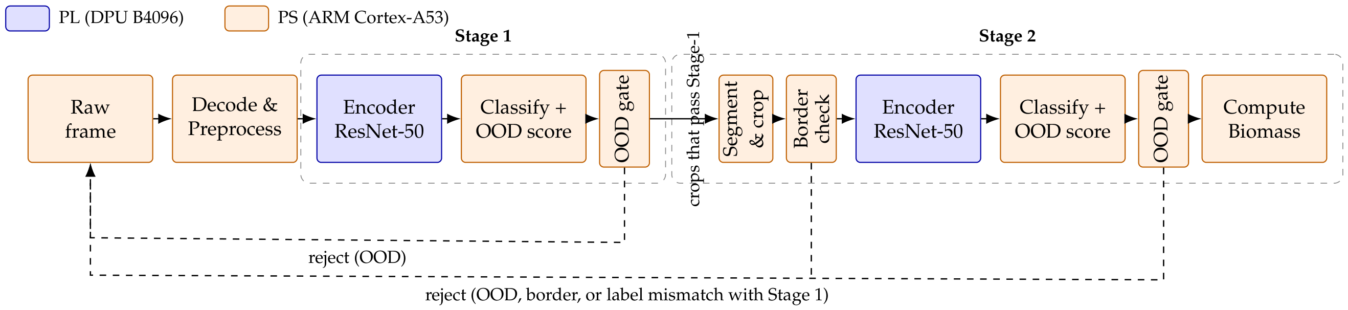
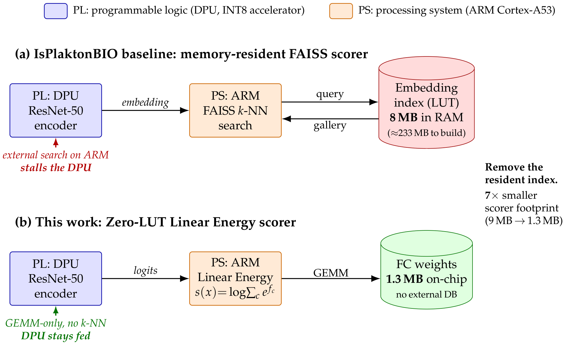
This work builds on IsPlanktonBIO [9], which turns each sensor crop into a verified taxonomic label and, ultimately, a biomass estimate through a two-stage cascade. We adopt that cascade and add the two elements it lacks for autonomous edge operation: an OOD gate at each stage, and a scorer light enough to drive those gates without a memory-resident gallery. Our contribution is therefore this open-set extension together with its hardware–software partition on the Kria KV260, both shown in Figure 2. Each raw crop is decoded and preprocessed on the ARM Cortex-A53 cores (processing system, PS) and passed directly to Stage-1, where a ResNet-50 backbone accelerated on the DPU (programmable logic, PL) assigns its taxonomic group and an OOD gate rejects the crop when its OOD score falls below a calibrated threshold. Both stages share the same OOD scorer, which computes that score as a cosine similarity for the FAISS baselines, or as a Linear Energy score for the deployed configuration. Crops that pass Stage-1 enter Stage-2, where an OpenCV (v4.8.0) segment_and_crop routine delineates the object inside the crop. A boundary check then discards specimens the frame has truncated: the pipeline rejects any segmentation touching more than one image border, and accepts a single-border contact only when it spans at most 10% of the image width. An independently trained ResNet-50 verifier, with its own OOD gate, classifies the surviving segmentation. The object is accepted only when both gates pass and the Stage-2 label agrees with the Stage-1 classification; the pipeline then estimates its biomass from the segmented area. This taxonomic agreement check, rather than a simple label hand-off, is what makes the cascade a verification pipeline.

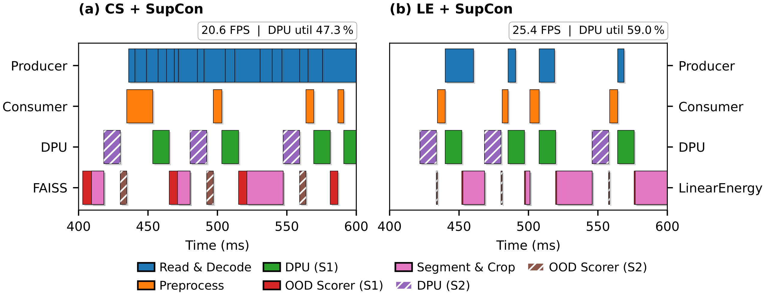
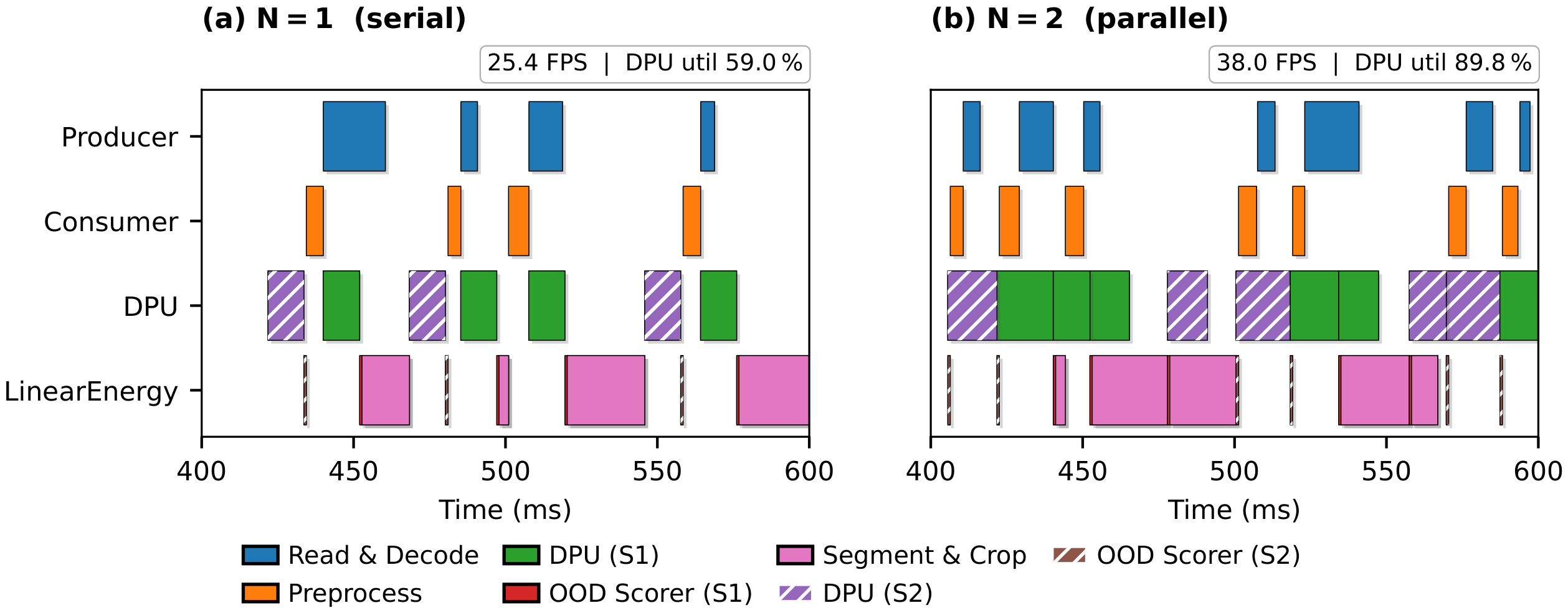
The workload is partitioned to keep the DPU saturated. The four Cortex-A53 cores host the decoding, preprocessing, segment_and_crop, OOD-scoring and orchestration threads, while the PL DPU accelerates the two ResNet-50 backbone inferences; all models are quantised to INT8 for DPU execution. At runtime the system is a multithreaded producer–consumer pipeline (Producer, Consumer, DPU multiplexer and scorer threads, visible in Figure 5, Section 4.2.2), with a semaphore-controlled count of in-flight images (pipeline_depth) that we exploit in Section 4.2.3. This partition is where the co-design constraint bites: the OOD scorer runs on the ARM cores in the interval between the two DPU calls, so it must be light enough not to stall the DPU. That requirement, rather than raw detection accuracy, is what motivates the Zero-LUT Linear Energy head over a FAISS look-up-table search (Section 3.5 and Section 4.2.2).

3.2. Dataset Partitioning and OOD Selection Rationale

Autonomous plankton monitoring systems must distinguish established biological classes from unforeseen taxonomic shifts. We structured the DYB-PlanktonNet dataset [2], a collection of in situ dark-field plankton images, to isolate routine classification performance from out-of-distribution (OOD) detection. The core In-Distribution (ID) dataset consists of 40,616 images spanning 78 taxonomic classes with the heavy long-tailed imbalance characteristic of in situ plankton imaging, partitioned into training (28,397 images), validation (6091 images), and testing (6128 images) subsets (approximately 70/15/15). We stratified this split by class: the training fraction stays close to 70% for every one of the 78 classes, and at least two images remain in both validation and test for each one, avoiding accidental zero-shot exclusion despite this long-tailed imbalance.

Alongside this in-distribution split, we curated an independent OOD set of 6803 images to represent three distinct biological and technical challenges:

• Marginal Taxonomic Representation: We designated the entire Annelida group (classes 001–008, 3009 images) as OOD. Annelida are a marginal fraction of the zooplankton community in regions such as the Canary Islands [39], justifying their exclusion from training.
• Episodic Bloom Simulation: We excluded the pteropod Creseis acicula (class 071, 3762 images) from training to simulate mass-abundance events of morphologically distinct organisms not previously seen by the model.
• Stochastic Rarity and Few-shot OOD: We included five sparsely sampled copepod taxa (Monstrilloid, class 032; Calanoid Nauplii, 018; Harpacticoid, 028; Calanoid Type C, 021; and Oithona sp. A, 023; 32 images in total) to test the system’s sensitivity to extreme outliers where only minimal reference samples exist.

This design evaluates both intra-class morphological generalisation and the system’s sensitivity to biologically plausible but statistically rare organisms.

3.3. Model Training and Quantisation

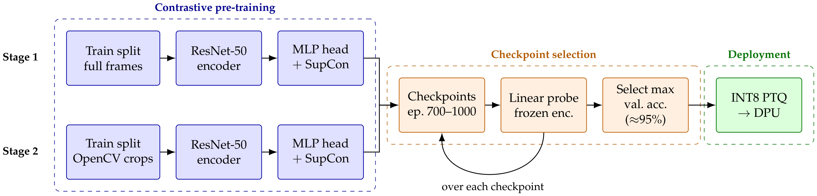
Full training details are given in the IsPlanktonBIO preprint [9]; we summarise the setup here, and in Figure 3, so that the present study is self-contained. Both stages use a ResNet-50 encoder [40] with a multi-layer perceptron (MLP) projection head, trained with the supervised-contrastive loss (SupCon) [41] for 1000 epochs with stochastic gradient descent (SGD, momentum 0.9, weight decay ${10}^{-4}$), a batch size of 32, and an initial learning rate of 0.016 (scaled linearly from the reference 0.5 at batch 1024) under a cosine schedule, with temperature $\tau =0.07$, on $224\times 224$ inputs and the standard SupCon augmentations. The Stage-1 encoder is trained on full frames and the Stage-2 encoder on the OpenCV-segmented crops, with independent weights and per-stage channel normalisation. From the loss plateau (epochs 700–1000) we train a linear-probing head separately on each frozen checkpoint and select the checkpoint whose head maximises validation accuracy; the selected backbones reach ≈95% closed-set validation accuracy. For deployment, the encoders and linear heads are quantised to INT8 [42,43] by post-training quantisation (PTQ) with the AMD Vitis-AI quantiser (v3.5.0) [16] and compiled to the DPU B4096 overlay. Every deployed INT8 backbone uses this PTQ path.

CIDER, the backbone evaluated alongside SupCon, follows its own reference implementation [32]: a ResNet-50 encoder with the same 128-dimensional MLP projection head, trained per stage on the same splits for 500 epochs with SGD (Nesterov momentum 0.9, weight decay ${10}^{-4}$), batch size 64, an initial learning rate of 0.1 under a cosine schedule, temperature $\tau =0.1$, and prototype exponential-moving-average factor $\alpha =0.95$. Its objective combines the dispersion and compactness terms, ${\mathcal{L}}_{\mathrm{dis}}+{\lambda }_c{\mathcal{L}}_{\mathrm{comp}}$, with ${\lambda }_c=1$. The 500-epoch budget, the temperature, the prototype factor and the embedding dimensionality are unmodified defaults of the CIDER reference implementation; we scaled down batch size and learning rate from their reference 512 and 0.5 to fit our single-GPU memory budget. CIDER’s encoder and head follow the same plain-PTQ path as SupCon’s, quantised via the Vitis-AI quantiser flow.

As an alternative end-to-end scorer, VOS [33] was trained on the segmented in-distribution crops with the reference implementation’s default configuration: a from-scratch ResNet-50 optimised by SGD (learning rate 0.05, batch size 64, Nesterov momentum 0.9, weight decay $5\times {10}^{-4}$, cosine schedule) for 100 epochs, with virtual-outlier synthesis from epoch 40 (a per-class feature queue of 1000 samples, 10,000 Gaussian candidates per class, the single lowest-density sample kept as the virtual outlier, and energy-regularisation weight 0.1). SupCon’s 1000-epoch budget and CIDER’s 500-epoch budget are, like VOS’s, unmodified defaults of their reference implementations, not a chosen asymmetry: each cosine schedule anneals its learning rate to near zero by the model’s own final epoch, so none of the three runs is truncated mid-schedule. We therefore compare the two methods as their respective authors configure them rather than under a matched training budget; VOS is, moreover, the only scorer we grant quantisation-recovery: PTQ with fine-tuning (PTQ + FT) or quantisation-aware training (QAT). Plain PTQ, without recovery, collapses VOS’s Stage-2 classifier to a single class (Table 10), whereas it leaves the deployed LE + SupCon scorer close to lossless (Table 4).

3.4. Open-Set Evaluation Protocol

Because the cascade makes two coupled decisions per image, accept or reject (is this a known plankton class or an out-of-distribution input?) and which class, a single closed-set accuracy is insufficient. We therefore report four complementary perspectives, each computed per stage and end-to-end, following conventions consistent across all variants.

Criterion 1: closed-set classification. Accuracy and macro-averaged Precision, Recall and F1 over in-distribution (ID) images only, with no OOD gating. Macro averaging weights every class equally, the honest choice for a 78-class taxonomic problem with heavy class imbalance. This criterion isolates raw discriminative power but, by construction, ignores the rejection decision: an image rejected by the energy gate still contributes its predicted class, so a change that improves OOD rejection has no mechanical path to raise this number.

Criterion 2: OOD detection. Threshold-independent AUROC (Area Under the Receiver Operating Characteristic curve) and FPR95 (false-positive rate at 95% ID true-positive rate), the standard separability metrics.

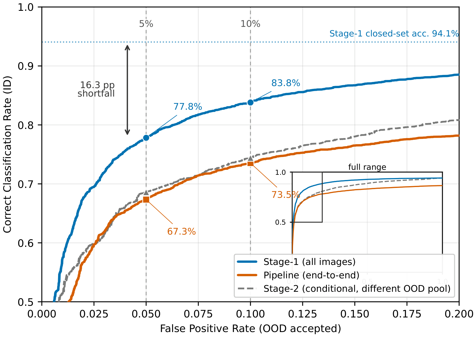
Criterion 3: open-set classification (headline). We adopt the Open-Set Classification Rate (OSCR) curve of Dhamija et al. [34]. Sweeping a score threshold $\theta$, the curve plots the Correct Classification Rate (CCR) against the False Positive Rate (FPR),

$$\begin{array}{cc}\hfill \mathrm{CCR}\left(\theta \right)& ={\displaystyle \frac{\left|\{x\in D_{\mathrm{ID}}:\arg {\max }_c{f}_c\left(x\right)=\widehat{c}\wedge s\left(x\right)\ge \theta \}\right|}{|D_{\mathrm{ID}}|}},\hfill \\ \hfill \mathrm{FPR}\left(\theta \right)& ={\displaystyle \frac{\left|\{x\in D_{\mathrm{OOD}}:s\left(x\right)\ge \theta \}\right|}{|D_{\mathrm{OOD}}|}},\hfill \end{array}$$

(1)

where $D_{\mathrm{ID}}$ and $D_{\mathrm{OOD}}$ are the in-distribution and out-of-distribution test sets, x is a query image, and $\widehat{c}$ is its ground-truth class label. $f_c\left(x\right)$ is the raw classifier score (logit) the model assigns to class c, one of the C taxonomic classes, for image x, so $\arg {\max }_c{f}_c\left(x\right)$ picks out the class with the highest score. $s\left(x\right)$ is the OOD score, for which higher means more in-distribution: it can be computed either as the Linear Energy score defined in Section 3.5, or as the cosine similarity adopted in the FAISS baselines. $\theta$ is the threshold Equation (1) sweeps: an image with $s\left(x\right)<\theta$ is rejected as out of distribution. The predicted label $\arg {\max }_c{f}_c\left(x\right)$ and the score $s\left(x\right)$ are read off the same forward pass. Dhamija et al.’s original formulation always sets $s\left(x\right)$ to the maximum softmax probability; we generalise it so that $s\left(x\right)$ can be any OOD score, and neither of ours is a softmax probability. An ID sample therefore contributes to CCR only if it is both accepted and correctly classified. Following Dhamija et al., we summarise the OSCR curve by reporting CCR at fixed operational leakage budgets, $\mathrm{CCR}@\mathrm{FPR}=5\%$ and $10\%$, the most intuitive deployment-facing figures and our primary open-set metric. As the threshold relaxes, CCR rises toward the closed-set accuracy; the shortfall at a fixed leakage budget is precisely the classification performance forfeited to imperfect OOD rejection.

Criterion 4: calibrated operating point. At the deployed threshold we report the True Positive Rate (TPR), FPR, the True Negative Rate (TNR) and the False Negative Rate (FNR), and, most importantly, the accuracy on accepted images, the user-facing quality of the system actually running on the DPU. Admission at this operating point is a compound criterion, not a single score threshold: an image must pass its stage’s OOD gate, its segmentation must not touch the image border, and the Stage-2 label must agree with Stage-1 at the pipeline level. Table 17 decomposes the resulting rejection rate on the Kria deployment into these four mechanisms.

Stage conventions. Stage-1 is evaluated over all images. Stage-2 is evaluated conditionally, only on images that passed the Stage-1 gate; its OOD pool is therefore restricted to the hardest OOD cases that already survived Stage-1, making its OOD metrics a conservative lower bound that is not directly comparable to Stage-1. In particular, a lower Stage-2 AUROC or a higher Stage-2 FPR95 than Stage-1 reflects this harder, pre-filtered OOD population and must not be read as Stage-2 being a weaker detector. The pipeline uses the best available prediction (Stage-2 when reached, else Stage-1) and the conservative combined score $\min (s_1,s_2)$, mirroring the two-gate accept logic in which an image is admitted only if both gates pass. Scores follow a common convention: whether a cosine similarity or an energy, higher means more in-distribution.

Statistical reporting. All metrics are point estimates on the fixed 6128-image test set. We quantify their sampling uncertainty with 95% bootstrap confidence intervals (CIs; 1000 resamples of the ID and OOD test sets), computed separately for the FP32 selection sweep (Table 2 and Table 3) and the INT8 deployment sweep (Table 4, Table 5, Table 6, Table 7, Table 8 and Table 9). Across the four FP32 scorers, half-widths range 0.8–0.9 pp for accuracy, 0.3–0.5 pp for AUROC, 1.0–1.5 pp for CCR@FPR and 2.6–3.8 pp for FPR95; for the INT8 variants, typical half-widths at the pipeline level are ±0.9 pp for accuracy, ±0.5 pp for AUROC, ±1.5 pp for CCR@FPR and ±3.5 pp for FPR95, with the conditional Stage-2 intervals wider on their smaller sample. Paired accuracy comparisons between variants use McNemar’s test on the same test images.

3.5. Backbone Selection and OOD Scoring Compatibility

We evaluated two contrastive training objectives as candidate backbones: Supervised Contrastive Learning (SupCon) [41] and Compactness and DispErsion Regularised learning (CIDER) [32]. Both architectures share a ResNet-50 encoder; they differ in the geometry of the learned embedding space and in the structure of the inference-time classification head.

When combined with a FAISS cosine-similarity (CS) scorer [44], both backbones reach their strongest OOD separation (Section 4.1), but only by keeping the memory-resident index that stalls the DPU. To satisfy the zero-external-memory deployment constraint, we evaluated the Energy Score [28] as a GEMM-only OOD scorer for both backbones:

$$s\left(x\right)=\log {\displaystyle \sum _{c=1}^C}\exp f_c\left(x\right)$$

(2)

where $f_c\left(x\right)$ is the c-th logit produced by the classification head. With the SupCon backbone, $f_c\left(x\right)$ is the output of a separately trained linear head (Linear Probing). With the CIDER backbone, $f_c\left(x\right)$ is the temperature-scaled cosine similarity between the query embedding and the c-th class prototype, which we label the prototype head. This second pairing proves problematic, for the reason set out next.

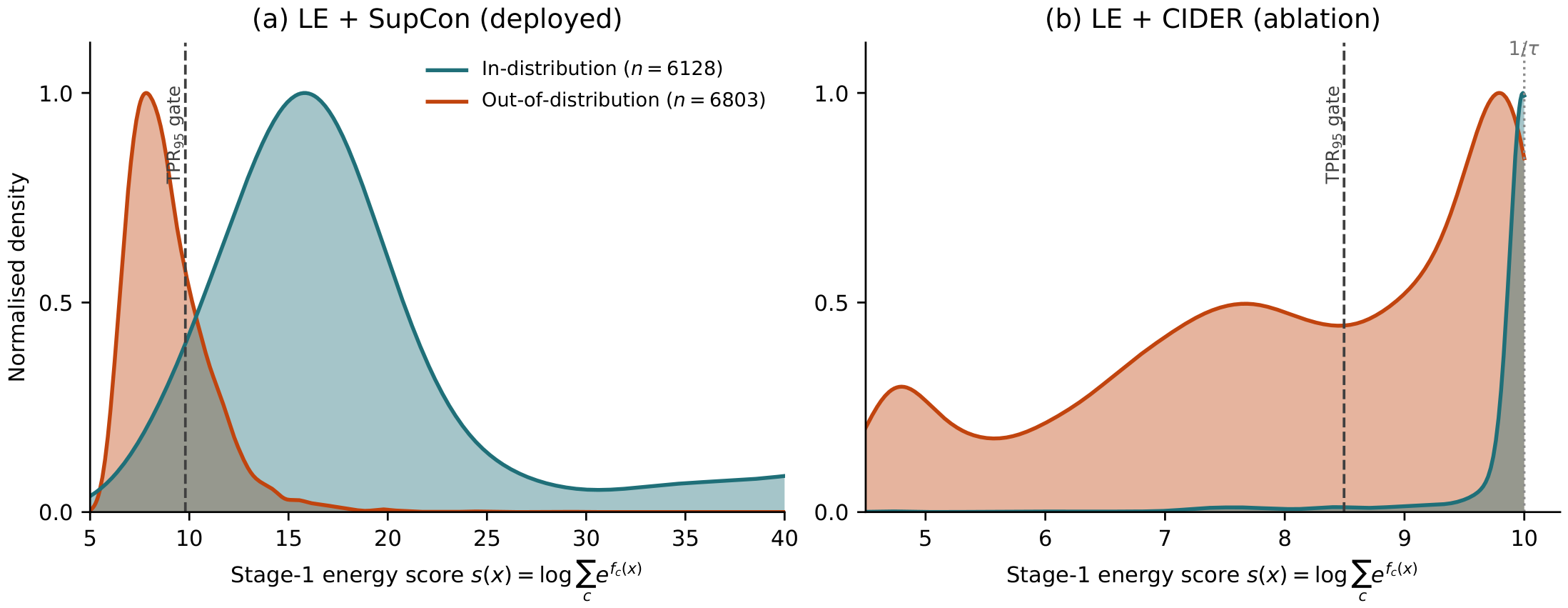
The difficulty is a geometric incompatibility rooted in the range of the logits each backbone feeds to the Energy Score. With CIDER the logits are the temperature-scaled cosine similarities to the class prototypes, $f_c\left(x\right)=\cos (z,{\mu }_c)/\tau$, which the unit-hypersphere geometry bounds to $[-1/\tau ,+1/\tau ]$ ($\pm 10$ at $\tau =0.1$). Because CIDER’s dispersion objective makes a single prototype dominate the sum, the LogSumExp in Equation (2) approaches the largest logit and is therefore effectively capped at $+1/\tau$. In-distribution objects, which align almost perfectly with their own prototype, should therefore concentrate at that ceiling, compressing the score’s dynamic range and leaving the OOD gate a narrow band to work in. SupCon, by contrast, classifies with an unbounded linear head, so in-distribution objects reach high energy while off-manifold OOD objects produce uniformly low logits, preserving a wide separating margin. Section 4.1 tests this prediction, and asks whether the logit bound alone accounts for it.

This analysis identifies LE + SupCon, a SupCon backbone with a linear classification head, as the deployed architecture. Its OOD gate operates at TPR₉₅: we set the energy threshold to the 5th percentile of the in-distribution validation scores, so that 95% of legitimate ID samples pass the gate, matching the FPR95 convention used throughout the OOD literature. This is a per-stage target on the validation split rather than an end-to-end acceptance rate. The FP32/GPU evaluations (Table 2 and Table 3) use this TPR₉₅ operating point directly; for on-device deployment, however, we recalibrate the Stage-1 and Stage-2 thresholds directly on the Kria INT8 model, because quantisation shifts the score distribution and FP32 thresholds do not transfer. Two compounding factors then separate the 95% target from what the deployed pipeline actually realises: both gates must independently pass, and the recalibrated threshold is evaluated on the test set rather than the validation split it was calibrated on (Section 4 reports the resulting operating point). We emphasise that deploying LE + SupCon is a deployability decision rather than a claim of OOD superiority: the FAISS cosine-similarity scorers separate OOD inputs more accurately (Table 2), but only the energy head satisfies the platform’s zero-external-memory, DPU-friendly constraint.

Beyond these two post hoc scorers, we also evaluated VOS as an end-to-end alternative that would remove the FAISS LUT search from both stages of IsPlanktonBIO entirely (its training and quantisation are detailed in Section 3.3). VOS estimates a class-conditional Gaussian over the penultimate-layer features, aggregates an object-level free energy via a class-reweighted LogSumExp in the spirit of Equation (2), and adds a learned nonlinear transform together with a virtual-outlier regulariser sampled from the low-likelihood tails of that Gaussian. Unlike the two post hoc scorers, it requires virtual-outlier training, and its INT8 deployment exposes a quantisation preprocessing pitfall specific to background-dominated inputs. We report the full comparison, together with this deployment finding, in Section 4.2.5 (Table 10); it does not displace LE + SupCon, which we retain as the deployed configuration.

4. Results

This section validates the deployability decision of Section 3.5, culminating in the quantised deployment on the Kria KV260 that confirms it holds under INT8, pipelined, resource-constrained conditions.

4.1. Algorithmic Performance (FP32/GPU Evaluation)

Before committing a scorer to hardware, we quantify what each candidate scorer costs and delivers in isolation. Table 2 reports this FP32 benchmark, evaluated end-to-end, on a workstation GPU (an NVIDIA GeForce RTX 3060). The FAISS cosine-similarity engines achieve the strongest separation between ID and OOD samples (CS + CIDER reaches an FPR95 of 23.6% and CS + SupCon 27.5%), ahead of the energy-score scorers (LE + SupCon 45.8%, LE + CIDER 51.7%), and the open-set CCR@FPR metric preserves the same ordering. Both LE + CIDER rows are ablations, discarded for the geometric reason set out in Section 3.5 and tested next. The decisive column, however, is Zero-LUT: only the energy-score scorers avoid the external FAISS index, whose PS-RAM nearest-neighbour search stalls the DPU at deployment (Figure 5, Section 4.2.2). LE + SupCon needs no external memory at all; LE + CIDER only partially so, since it still carries a small (≈82 kB) table of class-prototype vectors rather than a full embedding gallery.

Table 2. OOD-detection benchmark (FP32/GPU), pipeline-level and ordered by FPR95.

Method	AUROC	FPR95 ↓	CCR@5%	CCR@10%	Zero-LUT
CS + CIDER	96.03	23.64	77.48	81.72	No
CS + SupCon	95.82	27.53	77.76	81.03	No
LE + SupCon (TPR95, linear head)	93.07	45.77	70.95	76.43	Yes †
LE + CIDER (TPR95, prototype head) §	91.78	51.70	66.65	73.92	Partial ‡
LE + CIDER (TPR95, linear head) §	92.03	50.65	67.57	73.96	Yes †

Evaluated on 6128 ID/6803 OOD images. Zero-LUT: whether an external FAISS index is required at deployment. ^† No external memory. ^‡ Partial: small CIDER class-prototype vectors only, not a full embedding gallery. ^§ Ablation, not the deployed configuration. Bold: column-wise best. Differences smaller than the FP32-specific 95% bootstrap CIs of Section 3.4 (0.3–0.5 pp AUROC, 2.6–3.8 pp FPR95, 1.0–1.5 pp CCR@FPR) are not statistically distinguished.

Table 2. OOD-detection benchmark (FP32/GPU), pipeline-level and ordered by FPR95.

Method	AUROC	FPR95 ↓	CCR@5%	CCR@10%	Zero-LUT
CS + CIDER	96.03	23.64	77.48	81.72	No
CS + SupCon	95.82	27.53	77.76	81.03	No
LE + SupCon (TPR95, linear head)	93.07	45.77	70.95	76.43	Yes †
LE + CIDER (TPR95, prototype head) §	91.78	51.70	66.65	73.92	Partial ‡
LE + CIDER (TPR95, linear head) §	92.03	50.65	67.57	73.96	Yes †

Evaluated on 6128 ID/6803 OOD images. Zero-LUT: whether an external FAISS index is required at deployment. ^† No external memory. ^‡ Partial: small CIDER class-prototype vectors only, not a full embedding gallery. ^§ Ablation, not the deployed configuration. Bold: column-wise best. Differences smaller than the FP32-specific 95% bootstrap CIs of Section 3.4 (0.3–0.5 pp AUROC, 2.6–3.8 pp FPR95, 1.0–1.5 pp CCR@FPR) are not statistically distinguished.

The Stage-1 energy distributions confirm the geometric prediction of Section 3.5 (Figure 4). CIDER’s in-distribution scores pile up against the $+1/\tau$ ceiling: the interquartile range, or how widely the middle 50% of in-distribution scores are spread, collapses to 0.04, against 7.40 for SupCon. Nearly every in-distribution image now receives almost the same score. This loss of dynamic range means no threshold can separate the 2.1% of OOD objects whose score also saturates at that same ceiling. The margin does not vanish; it degrades to a strictly worse operating curve (AUROC 91.78% versus 93.07%, Table 2), on which threshold placement turns brittle.

The bound alone, however, does not account for LE + CIDER’s shortfall. To test whether the $\pm 1/\tau$ cap rather than the CIDER embedding itself limits performance, we trained a separate unbounded linear head on the frozen CIDER encoder, via the same Linear Probing procedure used for SupCon. Removing the bound leaves the operating curve statistically indistinguishable from the prototype-head ablation, within the bootstrap confidence intervals of Section 3.4. CIDER’s hyperspherical embedding therefore limits Energy Score performance independently of how its logits are produced, because it is optimised for angular class separation [32] rather than for an energy-informative feature geometry.

Figure 4. Stage-1 Linear Energy score $s\left(x\right)$ for LE + SupCon (a) and LE + CIDER (b). In-distribution test set (green) versus OOD set (red), peak-normalised. Dashed line: TPR₉₅ gate; dotted line: the $1/\tau$ logit ceiling, which applies only to the prototype head.

Figure 4. Stage-1 Linear Energy score $s\left(x\right)$ for LE + SupCon (a) and LE + CIDER (b). In-distribution test set (green) versus OOD set (red), peak-normalised. Dashed line: TPR₉₅ gate; dotted line: the $1/\tau$ logit ceiling, which applies only to the prototype head.

On closed-set classification (Table 3) the evaluated scorer configurations lie within about one percentage point of one another, all near 87% accuracy. Moreover, all scorers lie within the FP32-specific 95% bootstrap CI for accuracy (0.8–0.9 pp, Section 3.4), so the closed-set differences here are not statistically distinguished. We can assume that the gap likely reflects noise rather than a real difference between the scorers. The same caveat applies to the closest pairs in Table 2. The deployed LE + SupCon posts the highest point estimate for accuracy (87.57%) and recall, statistically tied with the FAISS baselines; LE + CIDER’s linear-head ablation leads on precision and F1, ahead of CS + CIDER and LE + SupCon respectively, likewise within the CI. The energy head therefore matches the FAISS baselines on taxonomic classification while dispensing with the look-up table: the zero-external-memory scorer trades away OOD separation, not classification quality. This favourable trade (worse OOD separation, but no cost to accuracy, in exchange for a zero-external-memory scorer) motivates its selection as the deployed configuration (Section 3.5).

Table 3. Closed-set classification benchmark (FP32/GPU), macro-averaged.

Method	Accuracy (%)	Precision (%)	Recall (%)	F1 (%)
CS + CIDER	87.11	90.94	80.08	84.04
CS + SupCon	87.27	88.03	80.11	82.76
LE + SupCon (TPR95, linear head) †	87.57	90.70	80.75	84.15
LE + CIDER (TPR95, prototype head) §	87.19	88.37	79.91	82.45
LE + CIDER (TPR95, linear head) §	87.37	91.02	80.75	84.22

Evaluated on 6128 test images. ^† Deployed configuration. ^§ Ablation, not the deployed configuration. Bold: column-wise best.

Table 3. Closed-set classification benchmark (FP32/GPU), macro-averaged.

Method	Accuracy (%)	Precision (%)	Recall (%)	F1 (%)
CS + CIDER	87.11	90.94	80.08	84.04
CS + SupCon	87.27	88.03	80.11	82.76
LE + SupCon (TPR95, linear head) †	87.57	90.70	80.75	84.15
LE + CIDER (TPR95, prototype head) §	87.19	88.37	79.91	82.45
LE + CIDER (TPR95, linear head) §	87.37	91.02	80.75	84.22

Evaluated on 6128 test images. ^† Deployed configuration. ^§ Ablation, not the deployed configuration. Bold: column-wise best.

4.2. Hardware Efficiency on the Kria KV260 (INT8 Evaluation)

The hardware measurements that follow, the memory footprint, latency and throughput, compression trade-offs and the cross-platform comparison, serve the transferable claims of this work rather than standing as a hardware benchmark in themselves. They establish that removing the memory-resident scorer keeps the accelerator fed, and that a quantised OOD-gated classifier must be characterised on the deployed INT8 model rather than assumed from its FP32 selection numbers.

The algorithmic metrics reported so far (Table 2 and Table 3) are FP32 measurements on the workstation GPU (NVIDIA GeForce RTX 3060), used to select the deployed configuration. The deployment target, however, is the INT8 model on the Kria KV260. Before analysing hardware behaviour, Table 4 isolates what quantisation costs by placing the two regimes of the deployed LE + SupCon pipeline side by side. Quantisation is close to lossless on closed-set quality (accuracy −1.0 pp, macro-F1 −1.9 pp) but visibly harder on the rejection task (FPR95 +7.3 pp, CCR@FPR5% −3.6 pp), which is precisely why the OOD thresholds are recalibrated directly on the quantised model rather than transferred from FP32 (Section 3.5). All INT8 figures in the remainder of this section refer to this recalibrated on-device operating point; the FP32/GPU figures are never used to characterise the deployed system.

Table 4. Effect of INT8 quantisation and on-device threshold recalibration on the deployed LE + SupCon pipeline.

Regime	Acc (%)	Macro-F1 (%)	AUROC (%)	FPR95 (%) ↓	CCR@5% (%)	CCR@10% (%)
FP32/GPU (selection)	87.57	84.15	93.07	45.77	70.95	76.43
INT8/Kria (deployed)	86.54	82.29	91.77	53.09	67.33	73.54
$\Delta$	−1.03	−1.86	−1.30	+7.32	−3.62	−2.89

FP32 is the GPU evaluation (Table 2 and Table 3); INT8 is the Kria KV260 deployment after recalibration (Table 11). All metrics are end-to-end pipeline values on the DYB-PlanktonNet test set (6128 ID/6803 OOD images); Δ is INT8−FP32.

Table 4. Effect of INT8 quantisation and on-device threshold recalibration on the deployed LE + SupCon pipeline.

Regime	Acc (%)	Macro-F1 (%)	AUROC (%)	FPR95 (%) ↓	CCR@5% (%)	CCR@10% (%)
FP32/GPU (selection)	87.57	84.15	93.07	45.77	70.95	76.43
INT8/Kria (deployed)	86.54	82.29	91.77	53.09	67.33	73.54
$\Delta$	−1.03	−1.86	−1.30	+7.32	−3.62	−2.89

FP32 is the GPU evaluation (Table 2 and Table 3); INT8 is the Kria KV260 deployment after recalibration (Table 11). All metrics are end-to-end pipeline values on the DYB-PlanktonNet test set (6128 ID/6803 OOD images); Δ is INT8−FP32.

4.2.1. Memory Footprint

Deploying the FAISS cosine-similarity scorer on the Kria KV260 imposes a two-tier memory cost. At first run, or after any database update, the full FAISS IndexFlat must reside in PS RAM to build the compressed inverted-file product-quantised (IVFPQ) index. Each gallery is first pruned offline with the intra-class redundancy-removal algorithm of Yang et al. [8], at a similarity threshold of $T_S=0.94$ for CIDER Stage 1, $T_S=0.96$ for CIDER Stage 2, and $T_S=0.90$ for both SupCon stages; the counts below are these pruned, deployed galleries. This flat gallery holds one 2048-dimensional float32 embedding per training image ($N_{\mathrm{train}}\times D\times 4$ B, where $N_{\mathrm{train}}$ is the number of training images, $D=2048$ the embedding dimensionality, and B denotes bytes, so each float32 embedding component costs 4 B). Building it occupies 339.9 MB across both stages for the 41,490-vector CIDER gallery and 254.1 MB for the 31,017-vector SupCon gallery, with a one-time ARM Cortex-A53 conversion of 248 s and 187 s, respectively (IVFPQ parameters in Table 5). Once built, the compressed .ivfpq.bin cache and its SQLite label databases occupy only 10 MB of steady-state PS RAM (≈8 MB cache plus ≈ 1.6 MB labels); this lossy but compact index is the only memory-feasible option on the SoM. These footprints denote the external, scorer-specific memory that the OOD stage adds on top of the compiled model. They exclude the total resident-set size: the actual RAM footprint of the whole running process, dominated instead by the Vitis-AI runtime and frame buffers, which together total ≈ 246 MB on the Kria and are essentially invariant to the scorer (Table 15).

The Zero-LUT Linear Energy scorer removes this cost. It has no cold-start regime and no database dependency: its only runtime files are two flat FP32 weight matrices ($78\times 2048+78=625$ kB per stage, 1.3 MB total), a 7.0× reduction over the same-backbone CS + SupCon’s FAISS runtime footprint and 7.5× over CS + CIDER’s. The gap widens with scale, since the IndexFlat grows linearly with the corpus. At 10× the current training set, roughly 280,000 images after a multi-year deployment, the flat CIDER gallery would need ≈3.4 GB of PS RAM, beyond the KV260’s LPDDR4 budget, and ≈40 min to convert, whereas the linear head stays at 1.3 MB and absorbs new data by retraining alone. This corpus-independence carries a flexibility cost: adding a species requires retraining the head and recalibrating its OOD threshold, whereas a retrieval scorer simply appends the new reference embeddings to its gallery. The Zero-LUT design thus trades open-vocabulary extensibility for a small, fixed footprint, a favourable exchange for a fixed regional taxonomy but less so where the class set changes frequently.

Table 5. Memory footprint of the three inference methods on the AMD Kria KV260.

Component	CS + CIDER	CS + SupCon	LE + SupCon
Cold-start (one-time, on first run or database update)
FAISS IndexFlat (training gallery, Stage 1 + 2)	339.9 MB	254.1 MB	—
IVFPQ conversion time (ARM Cortex-A53)	248 s	187 s	—
Runtime steady-state (per inference session)
FAISS IVFPQ cache (Stage 1 + 2)	8.2 MB	7.5 MB	—
SQLite label databases (Stage 1 + 2)	≈1.6 MB	≈1.6 MB	—
Linear head weights (Stage 1 + 2)	—	—	1.3 MB
Total external PS-RAM (runtime)	≈9.8 MB	≈9.1 MB	1.3 MB
DPU xmodel per method (PL)	49 MB	49 MB	49 MB

Cold-start = PS-RAM required during first-run IVFPQ index construction (one-time, triggered on database update). Runtime = PS-RAM occupied per inference session once the IVFPQ cache is built. xmodel files reside in DPU-managed PL-side memory. IVFPQ parameters: nlist = 64, m = 64, nbits = 8, nprobe = 16.

Table 5. Memory footprint of the three inference methods on the AMD Kria KV260.

Component	CS + CIDER	CS + SupCon	LE + SupCon
Cold-start (one-time, on first run or database update)
FAISS IndexFlat (training gallery, Stage 1 + 2)	339.9 MB	254.1 MB	—
IVFPQ conversion time (ARM Cortex-A53)	248 s	187 s	—
Runtime steady-state (per inference session)
FAISS IVFPQ cache (Stage 1 + 2)	8.2 MB	7.5 MB	—
SQLite label databases (Stage 1 + 2)	≈1.6 MB	≈1.6 MB	—
Linear head weights (Stage 1 + 2)	—	—	1.3 MB
Total external PS-RAM (runtime)	≈9.8 MB	≈9.1 MB	1.3 MB
DPU xmodel per method (PL)	49 MB	49 MB	49 MB

Cold-start = PS-RAM required during first-run IVFPQ index construction (one-time, triggered on database update). Runtime = PS-RAM occupied per inference session once the IVFPQ cache is built. xmodel files reside in DPU-managed PL-side memory. IVFPQ parameters: nlist = 64, m = 64, nbits = 8, nprobe = 16.

4.2.2. Inference Latency and Throughput

All three deployed variants share nearly identical DPU inference time (Table 6). They differ chiefly in the ARM-hosted OOD scorer that runs between the two DPU calls, so a slower scorer directly starves the DPU. At 300 MHz, the FAISS Stage-1 cosine-similarity search averages 17.73 ms per query for CS + CIDER and 15.60 ms for CS + SupCon, both with heavy tails (p95 of 31.4 ms, worst case 243.8 ms) and both far above the 12.31 ms DPU Stage-1. The DPU therefore idles between tasks for a mean of 14.78 ms for CS + CIDER, and 13.51 ms for CS + SupCon, holding utilisation to 45.1% and 47.3% and throughput to 19.64 and 20.61 FPS (N = 6028 ID images, first 100 warm-up frames discarded). The smaller SupCon gallery (17,697 vs. 28,397 vectors) yields the faster scorer, confirming that the FAISS index size, not the backbone, governs the bottleneck. Figure 5 traces this schedule over a representative 400–600 ms window, with the four stages ordered top to bottom: image decoding (Producer), preprocessing (Consumer), DPU acceleration, and OOD scoring. The fourth row, however, is a single ARM thread that runs two distinct tasks in sequence, not one: segment_and_crop extracts the Stage-2 object crop from the segmentation mask (pink blocks), then the OOD scorer itself produces the score that drives the gate’s accept/reject decision (red and hatched-brown blocks). Section 4.2.3 reports their individual timings.

Replacing the FAISS scorer with the Zero-LUT Linear Energy head cuts the Stage-1 scorer from 17.73 to 10.35 ms and the Stage-2 scorer from 5.15 to 0.85 ms, shrinking the mean DPU idle gap from 14.78 to 8.56 ms (−42%). Utilisation then rises to 59.0% and throughput to 25.4 FPS, a gain of 29% over CS + CIDER, the best-separating FAISS baseline, and 23% over the same-backbone CS + SupCon. Table 6 gives the full per-stage breakdown.

Figure 5. Serial execution traces (pipeline_depth = 1) of the pipeline on the AMD Kria KV260 at 300 MHz, for (a) CS + SupCon and (b) LE + SupCon. Hatched bars denote Stage-2 tasks.

Figure 5. Serial execution traces (pipeline_depth = 1) of the pipeline on the AMD Kria KV260 at 300 MHz, for (a) CS + SupCon and (b) LE + SupCon. Hatched bars denote Stage-2 tasks.

Table 6. Per-stage latency breakdown of the three OOD-scoring variants deployed on the AMD Kria KV260.

Stage	CS + CIDER		CS + SupCon		LE + SupCon
	Mean (ms)	p95 (ms)	Mean (ms)	p95 (ms)	Mean (ms)	p95 (ms)
DPU Inference — Stage 1	12.31	15.06	12.23	14.83	12.69	16.14
OOD Scorer — Stage 1 a	17.73	31.45	15.60	30.13	10.35	23.34
DPU Inference — Stage 2	11.93	12.13	11.95	12.17	11.95	12.16
OOD Scorer — Stage 2 a	5.15	6.39	4.76	5.35	0.85	0.84
DPU inter-task idle (mean)	14.78		13.51		8.56
DPU utilisation (%)	45.1		47.3		59.0
FPS	19.64		20.61		25.36

^a FAISS cosine-similarity search (CS variants); LogSumExp over linear-head logits (LE + SupCon). Stage 2 fires on images that pass the Stage 1 gate: 89.2%, 89.5%, and 88.7% of images for CS + CIDER, CS + SupCon, and LE + SupCon, respectively. DPU B4096 at 300 MHz, measured over N = 6028 test images (first 100 warm-up frames discarded). Mean and 95th-percentile (p95) latencies are reported for each stage. DPU inter-task idle = total DPU idle time ÷ total DPU invocations (Stage 1 + Stage 2 combined). DPU utilisation = DPU active time ÷ wall-clock time.

Table 6. Per-stage latency breakdown of the three OOD-scoring variants deployed on the AMD Kria KV260.

Stage	CS + CIDER		CS + SupCon		LE + SupCon
	Mean (ms)	p95 (ms)	Mean (ms)	p95 (ms)	Mean (ms)	p95 (ms)
DPU Inference — Stage 1	12.31	15.06	12.23	14.83	12.69	16.14
OOD Scorer — Stage 1 a	17.73	31.45	15.60	30.13	10.35	23.34
DPU Inference — Stage 2	11.93	12.13	11.95	12.17	11.95	12.16
OOD Scorer — Stage 2 a	5.15	6.39	4.76	5.35	0.85	0.84
DPU inter-task idle (mean)	14.78		13.51		8.56
DPU utilisation (%)	45.1		47.3		59.0
FPS	19.64		20.61		25.36

^a FAISS cosine-similarity search (CS variants); LogSumExp over linear-head logits (LE + SupCon). Stage 2 fires on images that pass the Stage 1 gate: 89.2%, 89.5%, and 88.7% of images for CS + CIDER, CS + SupCon, and LE + SupCon, respectively. DPU B4096 at 300 MHz, measured over N = 6028 test images (first 100 warm-up frames discarded). Mean and 95th-percentile (p95) latencies are reported for each stage. DPU inter-task idle = total DPU idle time ÷ total DPU invocations (Stage 1 + Stage 2 combined). DPU utilisation = DPU active time ÷ wall-clock time.

4.2.3. Pipeline Parallelisation

The deployed LE + SupCon runtime spreads work across four threads that communicate through bounded first-in–first-out (FIFO) queues: a producer decodes frames, a consumer preprocesses them, a mux thread dispatches Stage-1 and Stage-2 inferences to the single DPU core, and a scoring thread runs segment_and_crop and LinearEnergy on the ARM CPU. A counting semaphore governs how many images enter the pipeline at once (the pipeline_depth parameter) and holds the remainder back at the producer. Initialised to 1, it admits a single image to the DPU–LinearEnergy–DPU chain at a time, so the stages run in strict succession. At 300 MHz, DPU Stage-1 and Stage-2 inference require 12.69 ms and 11.95 ms per image, while the ARM CPU executes segment_and_crop (9.48 ms mean) and LinearEnergy scoring (10.35 ms + 0.85 ms) sequentially in the intervals between DPU calls. The DPU idles for a mean of 8.56 ms per task and achieves 59.0% utilisation in this configuration (Table 7).

Setting pipeline_depth: 2 in the YAML configuration raises the semaphore count to 2, so a second image can be preprocessed on the ARM CPU while the first is still traversing the DPU–LinearEnergy–DPU chain, overlapping the two processors ($N=2$ images in flight). Table 7 shows that $N=2$ raises DPU utilisation from 59.0% to 89.8% (+30.8 pp), cuts the mean inter-task idle gap from 8.56 ms to 1.41 ms (83.5% reduction), and increases throughput from 25.4 to 38.0 FPS (+50%). This effect is visible in Figure 6: at $N=2$ the DPU row is densely packed with back-to-back Stage-1 and Stage-2 inferences, whereas at $N=1$ visible gaps separate them. The residual 1.41 ms idle reflects ARM scheduler jitter rather than a structural pipeline stall, so admitting further images yields little further gain. We evaluated pipelining only for LE + SupCon; the FAISS baselines were not re-run at pipeline_depth: 2, so the 19.6-to-38.0 FPS improvement reported in Section 1.2 reflects the combined effect of removing the LUT and enabling pipelining, not the scorer swap in isolation. Pushing throughput higher would require either a larger DPU or moving CPU-side stages such as segment_and_crop into programmable logic; the B4096 configuration, however, already occupies most of the KV260 fabric (Section 4.2.7), leaving no room for either on this device. $N=2$ is therefore the practical operating point for this MPSoC.

Table 7. Effect of pipeline depth on DPU utilisation and throughput for LE + SupCon on the AMD Kria KV260.

Metric	N = 1 (Serial)	N = 2 (Parallel)	Change
Throughput (FPS)	25.4	38.0	+50%
DPU utilisation (%)	59.0	89.8	+30.8 pp
DPU inter-task idle gap (ms)	8.56	1.41	−83.5%

DPU B4096 at 300 MHz, N = 6128 images. FPS computed from Chrome trace events over a representative steady-state window; consistent with the 38.1±0.16 FPS 10-run mean reported in Table 8.

Table 7. Effect of pipeline depth on DPU utilisation and throughput for LE + SupCon on the AMD Kria KV260.

Metric	N = 1 (Serial)	N = 2 (Parallel)	Change
Throughput (FPS)	25.4	38.0	+50%
DPU utilisation (%)	59.0	89.8	+30.8 pp
DPU inter-task idle gap (ms)	8.56	1.41	−83.5%

DPU B4096 at 300 MHz, N = 6128 images. FPS computed from Chrome trace events over a representative steady-state window; consistent with the 38.1±0.16 FPS 10-run mean reported in Table 8.

4.2.4. Compression Trade-Offs

The INT8 baseline already meets the real-time target once parallelised (Table 7), so compression is justified only where a deployment demands higher throughput or a tighter power envelope, such as a battery-powered drifting buoy. Table 8 sweeps four hardware-aware reductions of the SupCon backbone at the deployed operating point (pipeline_depth: 2); we deploy none of them, so the sweep’s worth is the trade-off it exposes rather than a faster network. On efficiency, Once-For-All (OFA) [45] is the clear winner: at roughly half the baseline’s size (11.4 M params and 1.92 GFLOPs per stage vs. 23.5 M and 4.09 GFLOPs) it reaches 49.0 FPS at 7.21 W, a +28% throughput gain and a 30% cut in energy per image (0.147 vs. 0.212 J), and at 150 MHz (36.0 FPS, 5.83 W) it nearly matches the baseline’s 300 MHz throughput at 28% less power, a viable low-power mode. The two AMD Vitis-AI pruning variants [16] (iterative, one-step) and fastNAS (a latency-constrained Neural Architecture Search (NAS) sub-net from the NVIDIA TensorRT Model Optimizer [46]) form a middle cluster at 42–44 FPS (≈+12%), while the unpruned baseline is the slowest and most power-hungry (38.1 FPS, 8.07 W).

These efficiency gains, however, are not free: on closed-set quality the ranking inverts entirely. The baseline leads every metric (86.54% accuracy, 82.29% F1), with iterative pruning its only statistical equal on accuracy at 86.47%, significantly ahead of one-step’s 85.17% (McNemar’s test $p<0.001$). The lighter sub-nets pay more: OFA drops to 84.14% accuracy (−2.4 pp) and 74.12% F1 (−8.2 pp), and fastNAS is worst, its recall collapsing to 65.98% (F1 71.21%). This over-aggressive sub-net discards features the two-stage verification depends on.

Table 8. Hardware efficiency of the SupCon backbone under progressive compression, evaluated on the AMD Kria KV260.

Model	Params (M) †	FLOPs (M) †	Acc (%)	Prec (%)	Rec (%)	F1 (%)	150 MHz		300 MHz
							FPS	W	FPS	W
INT8 (baseline)	23.51	4087	86.54	88.29	78.96	82.29	24.1	6.13	38.1	8.07
INT8 + iterative pruning	17.53	2805	86.47	87.02	77.35	80.22	29.0	6.11	42.9	7.78
INT8 + one-step pruning	17.55	2871	85.17	83.94	75.05	77.17	28.5	6.07	42.4	7.83
INT8 + OFA	11.36	1920	84.14	83.11	70.60	74.12	36.0	5.83	49.0	7.21
INT8 + fastNAS	13.23	2819	83.93	83.40	65.98	71.21	29.1	6.01	43.9	7.64

DPU B4096, pipeline_depth: 2. Accuracy, Precision, Recall and F1 are end-to-end two-stage pipeline metrics on the DYB-PlanktonNet test set (6128 images). FPS = mean throughput over the full test set (10 runs). W= mean SOM power sampled at 0.5 s intervals via Texas Instruments INA260. Bold: column-wise best. FLOPs are reported as multiply–accumulate operations (MACs). ^† Perstage (encoder only; linear head: 0.16M params, negligible). Params/FLOPs are architecture-level quantities, measured on the optimised FP32 checkpoint; they are invariant under INT8 quantisation, which alters numeric precision but not tensor shapes or operation counts.

Table 8. Hardware efficiency of the SupCon backbone under progressive compression, evaluated on the AMD Kria KV260.

Model	Params (M) †	FLOPs (M) †	Acc (%)	Prec (%)	Rec (%)	F1 (%)	150 MHz		300 MHz
							FPS	W	FPS	W
INT8 (baseline)	23.51	4087	86.54	88.29	78.96	82.29	24.1	6.13	38.1	8.07
INT8 + iterative pruning	17.53	2805	86.47	87.02	77.35	80.22	29.0	6.11	42.9	7.78
INT8 + one-step pruning	17.55	2871	85.17	83.94	75.05	77.17	28.5	6.07	42.4	7.83
INT8 + OFA	11.36	1920	84.14	83.11	70.60	74.12	36.0	5.83	49.0	7.21
INT8 + fastNAS	13.23	2819	83.93	83.40	65.98	71.21	29.1	6.01	43.9	7.64

DPU B4096, pipeline_depth: 2. Accuracy, Precision, Recall and F1 are end-to-end two-stage pipeline metrics on the DYB-PlanktonNet test set (6128 images). FPS = mean throughput over the full test set (10 runs). W= mean SOM power sampled at 0.5 s intervals via Texas Instruments INA260. Bold: column-wise best. FLOPs are reported as multiply–accumulate operations (MACs). ^† Perstage (encoder only; linear head: 0.16M params, negligible). Params/FLOPs are architecture-level quantities, measured on the optimised FP32 checkpoint; they are invariant under INT8 quantisation, which alters numeric precision but not tensor shapes or operation counts.

Open-set behaviour shows that OOD separability and open-set delivery move independently (Table 9). OFA is the paradox: it attains the best OOD separation of all variants (FPR95 40.6% vs. 53.1% for the baseline), yet delivers the fewest correctly-classified accepted images (CCR@FPR5% 57.1% vs. 67.3%), because CCR@FPR credits a sample only when it is both accepted and correctly labelled and so penalises OFA’s weaker classifier, the trade-off that FPR95 alone hides. Iterative pruning again preserves open-set quality best, at CCR@FPR5% 66.2% (−1.1 pp) and FPR95 54.4%; the other variants shed 6–10 pp of CCR@FPR5%, and fastNAS is weakest on both axes, the only one whose OOD separation also degrades (FPR95 60.7%). The open-set view thus reinforces the deployment decision. The uncompressed baseline maximises correctly-classified, OOD-screened throughput and remains the recommended configuration. OFA is the preferred fallback when power or throughput is the binding constraint; iterative pruning is the choice when compression must preserve open-set quality.

4.2.5. VOS as an End-to-End Alternative: The Quantisation Preprocessing Gap

We evaluated Virtual Outlier Synthesis (VOS) [33] as a single end-to-end classifier that, by scoring out-of-distribution samples directly from a learned free-energy head, would remove the FAISS LUT search from both stages of IsPlanktonBIO. In FP32 the model classifies the in-distribution test set at 80.94% end-to-end accuracy (Table 10), but its Stage-2 OOD separation is weak (conditional Stage-2 AUROC 61.3%), so that the combined pipeline reaches only 63.4% FPR95, already below the deployed LE + SupCon scorer before any quantisation is applied.

Table 9. Open-set OOD robustness of the SupCon backbone under progressive compression (INT8, AMD Kria KV260).

Model	AUROC	FPR95 ↓	CCR@5%	CCR@10%
INT8 (baseline)	91.77	53.09	67.33	73.54
INT8 + iterative pruning	91.42	54.43	66.20	72.13
INT8 + one-step pruning	90.52	55.21	61.15	68.46
INT8 + OFA	91.13	40.59	57.12	68.06
INT8 + fastNAS	89.20	60.72	59.37	65.99

At 300 MHz, reported at the end-to-end pipeline level for the same variants as Table 8 and Table 11. CCR@FPR (correct-classification rate at a fixed OOD-leakage budget; after Dhamija et al. [34]) is higher-is-better. All values in percentage points. These are pipeline-level estimates; their 95% bootstrap CIs (Section 3.4) are typically ±0.5 pp (AUROC), ±3.5 pp (FPR95) and ±1.5 pp (CCR@FPR). Bold: column-wise best.

Table 9. Open-set OOD robustness of the SupCon backbone under progressive compression (INT8, AMD Kria KV260).

Model	AUROC	FPR95 ↓	CCR@5%	CCR@10%
INT8 (baseline)	91.77	53.09	67.33	73.54
INT8 + iterative pruning	91.42	54.43	66.20	72.13
INT8 + one-step pruning	90.52	55.21	61.15	68.46
INT8 + OFA	91.13	40.59	57.12	68.06
INT8 + fastNAS	89.20	60.72	59.37	65.99

At 300 MHz, reported at the end-to-end pipeline level for the same variants as Table 8 and Table 11. CCR@FPR (correct-classification rate at a fixed OOD-leakage budget; after Dhamija et al. [34]) is higher-is-better. All values in percentage points. These are pipeline-level estimates; their 95% bootstrap CIs (Section 3.4) are typically ±0.5 pp (AUROC), ±3.5 pp (FPR95) and ±1.5 pp (CCR@FPR). Bold: column-wise best.

Table 10. VOS as an end-to-end replacement for the FAISS scorer, compared against the deployed LE + SupCon.

Configuration	Acc (%)	F1 (%)	AUROC (%)	FPR95 (%)	CCR@5% (%)	CCR@10% (%)
LE + SupCon (deployed)	86.54	82.29	91.77	53.09	67.33	73.54
VOS, FP32 (GPU)	80.94	73.69	86.56	63.43	51.32	61.04
VOS, INT8 (PTQ)	20.94 *	15.39 *	92.25 *	34.51 *	11.78 *	14.98 *
VOS, INT8 (PTQ + FT)	80.81	71.09	87.57	59.90	51.72	61.66
VOS, INT8 (QAT)	73.74	63.71	82.62	68.06	37.62	47.56
VOS, INT8 (QAT + FT)	79.28	67.00	81.78	71.84	37.31	48.19

DYB-PlanktonNet test set (6128 ID; 6803 OOD images). Accuracy and F1 are end-to-end two-stage cascade metrics; AUROC and FPR95 are combined-pipeline OOD scores (min(s1, s2)). INT8 rows are measured on the AMD Kria KV260 (DPU B4096, 300 MHz); PTQ= post-training quantisation, FT = calibration fine-tuning (fast_finetune), QAT = quantisation-aware training. Bold: best among usable configurations. * Plain PTQ leaves the Stage-2 classifier degenerate (Stage-2 accuracy 19.6%, collapsing to a single class); its apparently strong OOD columns (AUROC 92.25%, FPR95 34.51%) ride on the intact Stage-1 energy through the min(s1, s2) combination and do not reflect a usable end-to-end model.

Table 10. VOS as an end-to-end replacement for the FAISS scorer, compared against the deployed LE + SupCon.

Configuration	Acc (%)	F1 (%)	AUROC (%)	FPR95 (%)	CCR@5% (%)	CCR@10% (%)
LE + SupCon (deployed)	86.54	82.29	91.77	53.09	67.33	73.54
VOS, FP32 (GPU)	80.94	73.69	86.56	63.43	51.32	61.04
VOS, INT8 (PTQ)	20.94 *	15.39 *	92.25 *	34.51 *	11.78 *	14.98 *
VOS, INT8 (PTQ + FT)	80.81	71.09	87.57	59.90	51.72	61.66
VOS, INT8 (QAT)	73.74	63.71	82.62	68.06	37.62	47.56
VOS, INT8 (QAT + FT)	79.28	67.00	81.78	71.84	37.31	48.19

DYB-PlanktonNet test set (6128 ID; 6803 OOD images). Accuracy and F1 are end-to-end two-stage cascade metrics; AUROC and FPR95 are combined-pipeline OOD scores (min(s1, s2)). INT8 rows are measured on the AMD Kria KV260 (DPU B4096, 300 MHz); PTQ= post-training quantisation, FT = calibration fine-tuning (fast_finetune), QAT = quantisation-aware training. Bold: best among usable configurations. * Plain PTQ leaves the Stage-2 classifier degenerate (Stage-2 accuracy 19.6%, collapsing to a single class); its apparently strong OOD columns (AUROC 92.25%, FPR95 34.51%) ride on the intact Stage-1 energy through the min(s1, s2) combination and do not reflect a usable end-to-end model.

Deploying VOS in INT8 surfaced a host-side preprocessing bug that is not specific to VOS: its fix (round-to-nearest input normalisation) underlies every INT8 result in this paper, so the figures in the preceding sections are already on the corrected pipeline. The first INT8 build collapsed, with almost every object assigned to a single class. A layer-by-layer comparison of the on-device DPU activations against the bit-accurate simulator, however, showed cosine similarities of 0.94–0.99 across all layers (0.99 at the output logits), ruling out the quantiser, the compiled xmodel, and the DPU as the source. The cause was instead a preprocessing mismatch: the edge C++ converted normalised floats to int8 by truncation toward zero (static_cast<int>), whereas the reference image-processing library used at training and in the bit-accurate simulator (torchvision) rounds to nearest. Both stages route through the same conversion: a shared normalize_to_int8 routine derives a 256-entry lookup table from each stage’s own mean/scale constants and applies it via OpenCV’s cv::LUT. The same truncated output therefore recurs for every pixel sharing that raw value. The Stage-1 preprocessing thread calls it on the full image, and Stage-2 calls it again, with its own constants, immediately before each segmented crop is enqueued for DPU inference. Because Stage-2 crops are background-dominated (roughly 95% black mask), the zero-valued pixels that cover most of the input were biased by a systematic +1 least-significant bit (LSB) under truncation, a near-uniform offset large enough to tip the classifier to a single class. We therefore implemented the edge normalisation to emulate torchvision’s rounding (std::lround), realigning the device preprocessing with the reference pipeline and restoring correct multi-class behaviour without retraining the model. The lesson generalises to any INT8 deployment in which the host application itself produces the fixed-point input tensor, as the Vitis-AI DPU flow requires here. On such sparse, background-dominated inputs, the fixed-point input normalisation must replicate the rounding convention of the reference preprocessing library used at training and calibration. TensorRT on the Jetson (Section 4.2.8) and similar toolchains instead accept a floating-point input and quantise internally via a calibrated scale, so they have no equivalent host-side rounding step to get wrong. Section 4.2.6 quantifies this correction’s effect on the deployed LE + SupCon Stage-1 gate.

With preprocessing corrected, the comparison of quantisation strategies is clean (Table 10). Plain PTQ recovers Stage-1 but leaves Stage-2 too degraded to be usable (20.9% end-to-end accuracy); a calibration fine-tuning pass (PTQ + FT) restores FP32-level accuracy (80.8%, versus 80.9% in FP32), and the QAT variants land between the two (73.7% and 79.3%). Even in its best INT8 configuration, however, VOS trails the deployed LE + SupCon scorer on both classification accuracy (80.8% vs. 86.5%) and OOD separation (pipeline FPR95 59.9% vs. 53.1%; AUROC 87.6% vs. 91.8%), while additionally requiring virtual-outlier training and a post-quantisation fine-tuning stage. VOS is therefore deployable on the Kria, but it does not justify displacing LE + SupCon, which attains higher accuracy and stronger OOD separation through a simpler training and deployment path and without any external memory.

4.2.6. Open-Set Performance of the Deployed Cascade

Applying the open-set protocol of Section 3.4 to the deployed LE + SupCon cascade (INT8, Kria KV260, round-to-nearest preprocessing) yields the per-stage picture in Table 11; Figure 7 traces the corresponding Open-Set Classification Rate (OSCR) curve, the correct-classification rate over ID images against the false-positive rate of accepted OOD inputs as the rejection threshold sweeps. The value of the open-set view is immediate at Stage-1: closed-set accuracy is 94.06%, but once the rejection decision is folded in, at a 5% OOD-leakage budget the gate classifies only 77.8% of all ID images correctly (CCR@FPR5%); the 16.3 pp shortfall is precisely the classification performance forfeited to imperfect OOD rejection, a cost that the closed-set number alone hides. Relaxing the budget to 10% recovers part of it (83.8%).

Table 11. Open-set evaluation of the deployed LE + SupCon cascade (INT8, Kria KV260), per stage and end-to-end.

Stage	NID	NOOD	Acc (%)	Macro-F1 (%)	AUROC (%)	FPR95 (%)	CCR@FPR
							5%	10%
Stage-1 (all)	6128	6803	94.06	89.80	94.53	32.09	77.81	83.81
Stage-2 (cond.)	5433	1688	94.18	89.74	89.36	63.09	68.60	74.41
Pipeline	6128	6803	86.54	82.29	91.77	53.09	67.33	73.54

At 300 MHz. Point estimates on the fixed 6128-image test set; pipeline-level 95% bootstrap CIs are ±0.9 pp (Acc), ±0.5 pp (AUROC), ±3.5 pp (FPR95) and ±1.5 pp (CCR@FPR), with the conditional Stage-2 intervals wider.

Table 11. Open-set evaluation of the deployed LE + SupCon cascade (INT8, Kria KV260), per stage and end-to-end.

Stage	NID	NOOD	Acc (%)	Macro-F1 (%)	AUROC (%)	FPR95 (%)	CCR@FPR
							5%	10%
Stage-1 (all)	6128	6803	94.06	89.80	94.53	32.09	77.81	83.81
Stage-2 (cond.)	5433	1688	94.18	89.74	89.36	63.09	68.60	74.41
Pipeline	6128	6803	86.54	82.29	91.77	53.09	67.33	73.54

At 300 MHz. Point estimates on the fixed 6128-image test set; pipeline-level 95% bootstrap CIs are ±0.9 pp (Acc), ±0.5 pp (AUROC), ±3.5 pp (FPR95) and ±1.5 pp (CCR@FPR), with the conditional Stage-2 intervals wider.

The conditional Stage-2 row of Table 11 should be read with care: its lower AUROC (89.36% vs. Stage-1’s 94.53%) reflects the harder OOD population that already survived the Stage-1 gate, not a regression. We use this open-set protocol as the lens for the preprocessing and compression analyses that follow, where closed-set accuracy alone would be misleading.

The rounding correction of Section 4.2.5 also affects the deployed LE + SupCon Stage-1, evaluated over the full INT8 test set.

Table 12. Effect of the input-normalisation rounding fix on the deployed LE + SupCon Stage-1 (INT8, Kria KV260). Table 11 reports only the corrected (rounding) figures.

Configuration	Acc (%)	Macro-F1 (%)	AUROC (%)	FPR95 (%)	CCR@FPR
					5%	10%
Truncation (buggy)	93.86	89.19	93.58	35.65	73.66	81.36
Rounding (corrected)	94.06	89.80	94.53	32.09	77.81	83.81
$\Delta$	+0.2 pp	+0.6 pp	+1.0 pp	−3.6 pp	+4.2 pp	+2.5 pp

isolates this effect: closed-set accuracy is essentially unchanged (+0.2 pp), while every open-set metric improves. The largest gain is in CCR@FPR5% (+4.2 pp), four more percentage points of ID images correctly classified.

Figure 7. Open-Set Classification Rate (OSCR) curve of the deployed LE + SupCon cascade (INT8, AMD Kria KV260). Main axes zoomed to the deployment region (FPR ≤ 0.20, CCR ≥ 0.5); the inset shows the full 0–1 curve with that window boxed. Filled markers: reported CCR@FPR operating points [34]; dotted line: Stage-1 closed-set accuracy; dashed curve: conditional Stage-2.

Figure 7. Open-Set Classification Rate (OSCR) curve of the deployed LE + SupCon cascade (INT8, AMD Kria KV260). Main axes zoomed to the deployment region (FPR ≤ 0.20, CCR ≥ 0.5); the inset shows the full 0–1 curve with that window boxed. Filled markers: reported CCR@FPR operating points [34]; dotted line: Stage-1 closed-set accuracy; dashed curve: conditional Stage-2.

Because every open-set figure above is computed on a single curated OOD set, we checked that the rejection behaviour is not an artefact of one homogeneous population by decomposing that set into its three biologically distinct groups (Section 3.2) and re-evaluating the deployed pipeline on each (Table 13). The two large groups reject robustly, one scoring above and the other below the 91.8% aggregate AUROC, so the headline open-set numbers do not hinge on one OOD type. The few-shot rare-taxon group (32 images across five sparsely sampled copepod classes) is both the hardest and the noisiest: morphologically these copepod-like outliers sit closest to the in-distribution classes, so a larger fraction leaks through the gate. Rejection therefore generalises across a marginal taxonomic group and a mass-abundance bloom, while near-distribution few-shot outliers remain the limiting case, consistent with the known difficulty of near-OOD detection.

Table 13. Open-set robustness across the three OOD groups for the deployed LE + SupCon pipeline (INT8, Kria KV260).

OOD Group	Images	AUROC (%)	FPR95 (%)	Rejected (%)
Annelida (marginal taxon)	3009	93.7	43.9	87.7
Creseis acicula (bloom)	3762	90.3	60.3	90.3
Rare copepod taxa (few-shot)	32	87.8	71.9	68.8
All OOD (aggregate)	6803	91.8	53.1	89.0

AUROC and FPR95 are computed against the 6128-image ID test set; “rejected” is the fraction of each group turned away at the calibrated deployment gate. The last row is the full OOD set of Table 11.

Table 13. Open-set robustness across the three OOD groups for the deployed LE + SupCon pipeline (INT8, Kria KV260).

OOD Group	Images	AUROC (%)	FPR95 (%)	Rejected (%)
Annelida (marginal taxon)	3009	93.7	43.9	87.7
Creseis acicula (bloom)	3762	90.3	60.3	90.3
Rare copepod taxa (few-shot)	32	87.8	71.9	68.8
All OOD (aggregate)	6803	91.8	53.1	89.0

AUROC and FPR95 are computed against the 6128-image ID test set; “rejected” is the fraction of each group turned away at the calibrated deployment gate. The last row is the full OOD set of Table 11.

4.2.7. Resource Utilisation and Power

A defining constraint of the deployment is that the deep-learning accelerator leaves little programmable-logic headroom on this compact system-on-module.

Table 14. Post-route Vivado resource utilisation on the AMD Kria KV260 (xck26-sfvc784-2LV-c) for the deployed DPU B4096 overlay and the evaluated B3136 alternative.

Resource	B4096 (Deployed)		B3136 (Evaluated)
	Used	Util. (%)	Used	Util. (%)
CLB LUTs	54,253	46.32	48,423	41.34
CLB Tiles	12,477	85.23	10,891	74.39
Block RAM	75.0	52.08	52.0	36.11
URAM	64.0	100.00	64.0	100.00
DSPs	710.0	56.89	566.0	45.35

Both configurations leave URAM fully occupied; B4096 additionally pushes CLB tiles near their ceiling. B3136 frees CLB tiles and block RAM but sacrifices 20.3% of the DSPs (710 → 566), reducing DPU throughput by approximately 25–30% and hence not deployed.

reports the Vivado post-route resource utilisation of the deployed B4096 overlay on the Kria KV260 (xck26-sfvc784-2LV-c), alongside the evaluated B3136 alternative discussed below. The design saturates the on-chip URAM (100%) and pushes Configurable Logic Block (CLB)-tile occupancy to 85.2%, while LUTs, block RAM and DSPs sit near half of their budgets. At the deployed 300 MHz operating point the complete pipeline draws 8.07 W at the module (INA260, mean over the run; Table 15), within the sub-10 W envelope required by autonomous platforms.

This near-ceiling utilisation is not specific to our design: a closely related Zynq UltraScale+ deployment from the same platform family likewise saturates URAM (100%) and reaches 92% LUT occupancy at a comparable ≈5 W budget [21]. Two independent deep-learning overlays on this class of compact SoM therefore both run against the same URAM wall, corroborating our finding (Section 5) that offloading an additional non-trivial kernel such as the segmentation stage to the programmable logic is infeasible without first shrinking the DPU (the B3136 alternative in Table 14), which would forfeit more throughput than the offload recovers.

4.2.8. Platform Comparison: MPSoC Versus Embedded GPU

To place the MPSoC deployment in context, we ran the identical pipeline (LE + SupCon, INT8, batch-1, end-to-end) on an NVIDIA Jetson Orin Nano Super (8 GB; JetPack 7.2, L4T R39.2.0), using TensorRT (v10.16.2.10) with post-training INT8 calibration [47] to match the Kria. We measured throughput, module power, and energy per image over ten runs, alongside accuracy and open-set delivery (Table 15). Module power came from the VDD_IN rail via tegrastats, the like-for-like counterpart of the Kria’s INA260 module-power reading. We restrict the comparison to the Jetson’s 10 W and 15 W power modes, the range comparable to the Kria’s own ≈8 W module draw; higher-power modes (25 W, MAXN) were also measured but fall outside the power budget relevant to this platform comparison and are omitted here. Both platforms are timed at batch-1, the single-image regime an imaging buoy runs in.

Table 15. Deployed LE + SupCon pipeline (INT8, batch-1, end-to-end) on the AMD Kria KV260 MPSoC versus the NVIDIA Jetson Orin Nano Super (8 GB) embedded GPU.

Platform	Mode	FPS	Power (W)	Energy/img (J)	Acc (%)	F1 (%)	CCR@5%	CCR@10%	RAM (MB)
Kria KV260 (MPSoC)	—	38.1	8.07	0.212	86.54	82.29	67.33	73.54	246
Jetson Orin Nano Super	10 W	145.3	6.84	0.047	87.66	84.14	70.48	76.06	776
Jetson Orin Nano Super	15 W	162.0	8.70	0.054	87.66	84.14	70.48	76.06	775

Power is mean module power over the run; energy per image = power/throughput. Accuracy, macro-F1 and CCR@FPR are end-to-end figures on the DYB-PlanktonNet test/OOD sets, identical across the two Jetson power modes as properties of the INT8 model. RAM is total process resident-set size (Section 4.2.1), not the external scorer memory of Table 5.

Table 15. Deployed LE + SupCon pipeline (INT8, batch-1, end-to-end) on the AMD Kria KV260 MPSoC versus the NVIDIA Jetson Orin Nano Super (8 GB) embedded GPU.

Platform	Mode	FPS	Power (W)	Energy/img (J)	Acc (%)	F1 (%)	CCR@5%	CCR@10%	RAM (MB)
Kria KV260 (MPSoC)	—	38.1	8.07	0.212	86.54	82.29	67.33	73.54	246
Jetson Orin Nano Super	10 W	145.3	6.84	0.047	87.66	84.14	70.48	76.06	776
Jetson Orin Nano Super	15 W	162.0	8.70	0.054	87.66	84.14	70.48	76.06	775

Power is mean module power over the run; energy per image = power/throughput. Accuracy, macro-F1 and CCR@FPR are end-to-end figures on the DYB-PlanktonNet test/OOD sets, identical across the two Jetson power modes as properties of the INT8 model. RAM is total process resident-set size (Section 4.2.1), not the external scorer memory of Table 5.

The comparison is deliberately unflattering to our own platform: for pure inference the Orin Nano Super is markedly faster and more energy-efficient than the Kria: roughly $3.8\times$ the throughput at lower module power, and $4.5\times$ less energy per image (Table 15). We report this openly. Two qualifications frame the result without overturning it. First, the 2021 KV260 operates close to its resource ceiling (Section 4.2.7) against a newer, substantially more powerful 2023-generation module, so part of the gap is generational. Second, and more importantly, throughput is not the binding constraint: an imaging buoy captures a few frames per second, so both platforms exceed the requirement by more than an order of magnitude within the same sub-9 W envelope. The comparison also inverts on memory, the Jetson’s CUDA and TensorRT runtime occupying far more resident RAM than the Kria’s (Table 15), a scorer-invariant gap (Section 4.2.1) large enough to matter on a memory-constrained buoy controller. The value of this work therefore does not rest on winning an inference-efficiency benchmark, which goes to the Jetson, but on two things. First, its methodological contributions are platform-agnostic, as the Jetson port below reproduces. Second, specific to the MPSoC, its reconfigurable logic can host the imaging front-end, sensor interfacing and deterministic control alongside the accelerator, which a fixed-function GPU module cannot.

As on the Kria, the Jetson’s thresholds are recalibrated on its own quantised engine. Its host-side preprocessing stays in floating point (TensorRT calibrates internally), so the Kria’s truncation-versus-rounding pitfall (Section 4.2.5) has no counterpart and only the higher-level recalibration lesson transfers. The Jetson deployment reproduces the same accuracy and open-set behaviour, in fact slightly surpassing the deployed Kria on every metric of Table 15. We attribute that small margin to the two INT8 toolchains rather than the algorithm: the CCR gap exceeds the ±1.5 pp bootstrap CI, whereas the accuracy gap is marginal. This margin is not a case of INT8 outperforming full precision, either: against the FP32/GPU figures (Table 4) the Jetson is statistically indistinguishable on CCR@FPR, whereas the Kria’s quantisation does measurably cost open-set quality. Both platforms nonetheless correctly classify an identical 97.6% of accepted in-distribution images, at gate-acceptance rates of 82.9% and 83.6% respectively (

Table 16. Calibrated operating point of the deployed LE + SupCon cascade per platform (INT8, end-to-end).

Platform	TPR (%)	FNR (%)	TNR (%)	FPR (%)	Acc. on Accepted (%)
Kria KV260 (INT8)	82.9	17.1	89.0	11.0	97.56 (4956/5080)
Jetson Orin Nano Super (INT8)	83.6	16.4	88.4	11.6	97.62 (5004/5126)

TPR/FNR and TNR/FPR are complementary pairs (each sums to 100%); Acc. on accepted is the correctclassification rate among ID images admitted by the gate (correct/accepted counts in parentheses), with leaked OOD images excluded by construction.

), confirming that the scoring and evaluation methodology transfers across accelerators. We thus present the Kria as a valid, integration-oriented deployment target and the Orin Nano Super as a faster, more energy-efficient alternative for inference-only nodes: an honest platform trade-off, not a verdict.

Of the 6128 test-set ID images, the deployed Kria cascade rejects 17.1%, the complement of its 82.9% gate-acceptance rate (Table 16).

Table 17. Decomposition of the Kria KV260 in-distribution rejection rate by mechanism.

Rejection Mechanism	% of ID Images
Stage-1 OOD gate	5.1
Stage-2 OOD gate	2.8
Segmentation touches image border	6.2
Stage-1/Stage-2 label disagreement	3.0
Total	17.1

decomposes this in-distribution rejection rate by mechanism: only 7.9 pp (5.1% Stage-1 plus 2.8% Stage-2) are score-threshold rejections from the OOD gate itself, while the remaining 9.2 pp are geometric or consistency checks (6.2% border-touching segmentations, 3.0% Stage-1/Stage-2 label disagreement). Over half of all rejections therefore come from mechanisms other than the calibrated OOD gate, confirming that acceptance at this operating point is the compound criterion described in Criterion 4 (Section 3.4), not a single score threshold.

5. Discussion

This work shows that an out-of-distribution-aware, two-stage plankton classifier can run end-to-end on a compact AMD Kria KV260 MPSoC without any external look-up structure. Replacing the FAISS nearest-neighbour scorer with a GEMM-only Linear Energy head over a SupCon backbone (LE + SupCon) removes both the Processing-System bottleneck that stalled the DPU and the memory-resident embedding database, while matching the FAISS baselines on end-to-end classification accuracy (differences within the 95% bootstrap CI, Table 3). Competitive open-set plankton recognition therefore does not require a similarity gallery in RAM.

A recurring theme of our evaluation is that closed-set accuracy and OOD rejection are orthogonal axes, and that reporting either in isolation is misleading for an OOD-gated cascade. We therefore adopt the Open-Set Classification Rate of Dhamija et al. [34], summarised by CCR at a fixed leakage budget (Section 3.4). Two findings only become legible under this lens. First, correcting the input-normalisation rounding raises Stage-1 open-set quality (Table 12) even though closed-set accuracy is essentially unchanged. Second, the Once-For-All sub-net attains the best OOD separation of any variant (pipeline FPR95 40.6%) yet delivers the fewest correctly-classified accepted images (CCR@FPR5% 57.1%, Table 9), because its lighter backbone classifies less accurately. A FPR95-only reading would have ranked these cases backwards. We argue that CCR@FPR, which credits a sample only when it is both accepted and correctly labelled, should be the headline metric whenever an edge classifier couples recognition with rejection.

Two deployment-engineering lessons generalise beyond this application. The first is a quantisation preprocessing gap (Section 4.2.5). Host-side truncation, rather than the reference library’s rounding, biased the near-uniform background of Stage-2’s background-dominated crops enough to collapse the classifier. We traced this failure to preprocessing rather than the quantiser or the DPU, and confirmed the fix by matching the training library’s rounding convention. It applies to any INT8 toolchain in which the host itself produces the fixed-point tensor, but not to toolchains such as TensorRT on the Jetson (Section 4.2.8) that quantise internally from a floating-point input. The second lesson is that OOD thresholds do not transfer across precision: quantisation shifts the score distribution, so the TPR₉₅ operating point is recalibrated directly on the Kria INT8 model rather than inherited from the FP32 evaluation (Section 3.5).

These observations also explain why the alternative scorers were not deployed. The FAISS cosine-similarity engines achieve the strongest raw OOD separation (Table 2) but tie up the ARM thread with a high-latency index search (mean 17.7 ms, tails beyond 240 ms; Figure 5). Because this index search is not a neural-network operator, the DPU cannot run it. Although FAISS-style product-quantised retrieval can be mapped to custom programmable logic on larger FPGAs [48,49], the B4096 overlay already fills the KV260 fabric, leaving no room for such a kernel (Section 4.2.7). Pairing the Energy Score with a CIDER backbone fails for a structural reason: the unit-hypersphere geometry keeps OOD samples close to multiple class prototypes, inflating their free energy. Virtual Outlier Synthesis is genuinely deployable once the preprocessing is corrected and a fine-tuning pass is added, but even in its best INT8 configuration it trails LE + SupCon on both accuracy and OOD separation while demanding virtual-outlier training (Table 10); the simpler, post hoc Energy head is preferable.

Several limitations frame future work. With FAISS removed, the residual serial bottleneck is the ARM segment_and_crop stage (∼9.5 ms; Section 4.2.3); offloading it to programmable logic is attractive but, on this SoM, forces the DPU down to a B3136 overlay that sheds ∼20% of its DSPs and itself becomes the bottleneck (Section 4.2.7). A larger fabric with dedicated vector accelerators may shift this balance: AMD’s Versal adaptive SoC, for instance, could host the OOD scorer alongside the DPU and a High-Level Synthesis (HLS) segmentation kernel without contention. A further reconfigurability advantage is frequency scaling: the DPU can be synthesised to run at a range of clock rates, each with a distinct power draw (Table 8). The operating point can then be switched on a running system by reloading the programmable-logic configuration, without the reboot that changing the embedded GPU’s power mode required in our setup. On an energy-harvesting buoy this would let the instrument match its inference clock to the remaining energy budget. A future Versal-based generation could make such energy-adaptive inference a primary design axis for long-endurance marine sensors. Compression adds a further dimension. On this single-corpus sweep, OFA leads on OOD separability yet delivers the fewest correct acceptances (Section 4.2.4). This motivates compression-aware training whose objective targets open-set delivery (correct classification of accepted images) rather than the accuracy- or separability-driven criteria of the tools used here. Finally, our results come from a single SoM and the DYB-PlanktonNet distribution; in situ validation on the imaging buoy, across additional taxa and acquisition conditions, remains the natural next step.

6. Conclusions

Two lessons are the portable core of this work. First, edge classifiers that couple recognition with rejection should be evaluated with an open-set metric: closed-set accuracy and OOD separation are orthogonal, and the correct-classification rate at a fixed leakage budget (CCR@FPR) exposes trade-offs, such as a compressed sub-net with excellent OOD separation but poor useful throughput, that threshold-free OOD scores hide. Second, faithful INT8 deployment requires recalibrating OOD thresholds directly on the quantised model, since the score distribution shifts under quantisation regardless of toolchain. Wherever the host itself produces the fixed-point input tensor, as the Vitis-AI DPU flow requires here, it also requires matching the training preprocessing’s rounding convention. We confirm the threshold-recalibration lesson is platform-agnostic. The Jetson Orin Nano Super port needed no rounding fix, since its TensorRT toolchain quantises internally from a floating-point input rather than through host-side casting, yet it still required its own threshold recalibration, and it reproduces the same accuracy and open-set behaviour.

We established these lessons through a hardware–software co-design, on a compact AMD Kria KV260 MPSoC, of an open-set plankton classifier derived from the IsPlanktonBIO framework. Replacing the FAISS nearest-neighbour scorer with a GEMM-only Linear Energy head over a SupCon backbone lets the deployed pipeline run entirely on-device with no external look-up structure, reducing the runtime memory footprint roughly sevenfold (to 1.3 MB) and, after a single-parameter pipeline-parallelisation, sustaining 38.0 FPS at 89.8% DPU utilisation while matching the FAISS baselines on end-to-end classification accuracy (differences within the bootstrap CI). Two backbone–scorer alternatives were ruled out for well-founded reasons: CIDER through a hyperspherical-geometry incompatibility with the Energy Score, and Virtual Outlier Synthesis because, although deployable in INT8, it underperforms LE + SupCon on both accuracy and OOD separation at greater training cost. Future work will port the pipeline to AMD’s Versal adaptive SoC to relieve the residual segmentation bottleneck, explore compression-aware training that preserves open-set delivery, and validate the system in situ across broader plankton taxa.