Voltage–Current Curve-Based Line Protection for Renewable Energy Systems with Grid-Forming Inverters

Abstract

The increasing penetration of inverter-based renewable energy resources is reshaping transmission-line fault characteristics and weakening protection criteria designed for synchronous-generator-dominated grids. This paper proposes an internal-fault identification scheme based on voltage–current coupling characteristic curves (UICs) constructed from voltage and current measurements at both line terminals. Geometric descriptors of the UIC are used to build an ellipsoidal feature space representing normal operating conditions and external faults. Internal faults are identified from the normalized distance between the online feature vector and this space. A local voltage-transient startup criterion is also introduced, and current-transformer (CT) saturation correction is incorporated to reduce distortion in the measured currents. PSCAD simulations under different fault locations, transition resistances, fault types, noise levels, and CT-saturation conditions show that the proposed scheme distinguishes internal faults from external faults and normal operation reliably. Because the criterion depends on line-side coupling features rather than the short-circuit output of a specific power source, it is suitable for protection applications in renewable energy systems with grid-forming inverters.

1. Introduction

The rapid integration of renewable energy resources is changing power systems from synchronous-generator-dominated networks to networks with high shares of inverter-based resources [1,2,3,4]. During faults, these resources exhibit nonlinear and time-varying voltage, current, and impedance characteristics that differ from those of synchronous machines [5,6,7,8,9]. Grid-forming converters are especially important because they can provide fast power support, flexible regulation, and stronger support for weak grids. However, their fault response is governed by power-electronic hardware and control strategies. Current limiting, nonlinear transients, and weakened fault-current contribution make conventional relay protection less dependable and impose stricter requirements on protection speed, reliability, and selectivity.

Existing studies have addressed the reduced adaptability of transmission-line protection in grid-forming-resource systems from several perspectives. One approach is to design protection criteria from source-side fault-response features. Reference [10] combined an IIRES current-control strategy with distance protection to improve line protection for asymmetric faults in renewable-energy integration scenarios. Reference [11] analyzed protection behavior using the dynamic characteristics of fault current-limiting control and showed that control strategies strongly affect current output during faults. Reference [12] proposed an iterative short-circuit current calculation method that accounts for the voltage-controlled current-source characteristics of renewable energy resources. Reference [13] analyzed current phase characteristics on both sides of a photovoltaic transmission line and proposed a longitudinal protection method based on the Dice similarity coefficient. These methods improve fault discrimination by exploiting renewable-energy fault responses, but their performance remains closely tied to control strategies, current-limiting methods, and fault ride-through behavior. When the source operating mode or control parameters change, their adaptability still requires further validation.

A second research direction is to enhance fault detectability through active signal injection. Reference [14] identified fault zones in DC grids by injecting sinusoidal test signals of different frequencies through converters and analyzing the resulting response differences. Reference [15] proposed an impedance-phase-based active-injection method for radial VSC-HVDC grids, in which frequency-specific post-fault signals are used to determine whether the fault is inside or outside the protected zone. Although active-injection methods can create new discriminative features, they usually require additional signal sources or supplementary control loops. This increases hardware cost and complicates coordinated control-protection design. A third class of methods seeks criteria that are less sensitive to source characteristics. Reference [16] used line-parameter identification and fault-component information to reduce the impact of source-side fault variations. Reference [17] proposed a distance backup protection scheme based on a steady-state DC line model, and Reference [18] used early-fault information for parameter-identification-based distance protection of AC transmission lines. These methods reduce dependence on source-side fault output, but they often require accurate circuit models, high-quality sampling data, iterative solutions, differential calculations, or simplified line models. These requirements can slow the response and make engineering implementation more complex.

Although parameter-identification methods are relatively robust to source-side variations, iterative computation and simplified line modeling can still limit protection speed and reliability. To overcome these limitations, this paper proposes a three-dimensional voltage–current coupling characteristic curve (UIC) representation constructed from voltage and current measurements at both line terminals. The UIC shape features reflect changes in line topology and parameters. An ellipsoidal feature space is then established for normal operation and external faults using sample statistics, and internal faults are identified by comparing the measured UIC feature vector with this feature space. The proposed scheme is verified through PSCAD simulations. And this criterion is based on line topology and terminal coupling features, which makes it less directly dependent on source short-circuit capacity than conventional impedance-based protection.

2. The Impact of Grid-Forming Power Sources on Traditional Protection Systems

2.1. Fault Control Strategies for Grid-Forming Power Sources

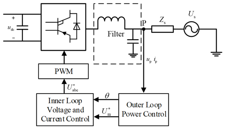
The objective of grid-forming control is to make the converter behave as a voltage source during grid-connected operation, in a manner similar to a synchronous machine. The converter can autonomously establish terminal-voltage magnitude and phase instead of relying on the external grid voltage for lock-in synchronization. A typical grid-forming controller contains an outer loop and an inner loop. The outer loop generates voltage-magnitude, frequency, or phase references, while the inner loop regulates voltage and current according to these references and produces drive signals through the PWM stage [19]. Figure 1 shows the basic structure of a grid-forming power source. Point P denotes the equivalent grid-connection point, θ is the voltage phase reference, $U_{\mathrm{m}}^{*}$ is the reference voltage amplitude, and $U_{\mathrm{abc}}^{*}$ is the three-phase voltage modulation waveform.

Grid-forming power sources commonly use droop control, virtual synchronous generator control, or synchronous power control to establish the outer-loop dynamics. Droop control emulates primary frequency and voltage regulation through active-power-frequency and reactive-power-voltage characteristics. Virtual synchronous generator control adds inertia and damping to improve dynamic support under disturbances. The power loop generates a frequency or phase reference, which is integrated to obtain θ. At the same time, the voltage loop produces the voltage reference $U_{\mathrm{m}}^{*}$. Together with the inner voltage and current loops, this reference regulates the common-coupling-point voltage. As a result, the grid-forming source exhibits the external behavior of a voltage source with controlled impedance during steady-state operation.

2.2. Impact of Grid-Forming Power Sources on Traditional Protection Methods

Grid-forming power sources establish terminal voltages actively through control methods such as droop control and virtual synchronous generator control. Their output can therefore be represented equivalently as a controlled voltage source in series with a virtual impedance. Unlike conventional synchronous sources, grid-forming sources usually apply current-limiting and voltage-support control during faults. The amplitude, phase, and transient evolution of the output current therefore depend strongly on the controller. Protection criteria derived from the short-circuit behavior of synchronous sources may consequently be unsuitable for grid-forming-source scenarios [20].

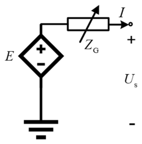
In terms of output characteristics, a grid-forming power source can be modeled as a controlled voltage source in series with an equivalent impedance, as shown in Figure 2. The port voltage can be approximated as

$${\dot{U}}_{\mathrm{s}}=E-Z_{\mathrm{G}}\dot{I}$$

(1)

In this equation, E is the voltage reference, Z_G is the virtual impedance, and $\dot{I}$ is the output current. When a system fault occurs, the fault current is constrained by the current-limiting element and satisfies Equation (2).

$$\left|{\dot{I}}_f\right|\le I_{\max }$$

(2)

During a fault, the voltage and current at both line terminals are limited. This changes the protection features available to conventional criteria and weakens the stable relationship between fault characteristics and operating thresholds. This effect is analyzed below using distance protection and differential protection as examples.

Distance protection typically relies on measured impedance to identify the faulted section, as shown in Equation (3).

$$Z_{\mathrm{m}}={\displaystyle \frac{{\dot{U}}_{\mathrm{m}}}{{\dot{I}}_{\mathrm{m}}}}$$

(3)

In traditional power grids, the measured impedance generally decreases as the fault approaches the relay, and its trajectory is relatively stable. After grid-forming power sources are integrated, voltage support, virtual impedance, and current-limiting control jointly affect the magnitude and phase of voltage and current. As a result, Z_m may deviate from the conventional setting trajectory and cause misoperation.

For current differential protection, one classic method is the percentage differential protection criterion based on braking characteristics [21], whose basic criterion can be expressed as

$$\left\{\begin{array}{l}{I}_{\mathrm{dif}}=\left|{\dot{I}}_1-{\dot{I}}_2\right|\\ I_{\mathrm{res}}={\displaystyle \frac{\left|{\dot{I}}_1\right|+\left|{\dot{I}}_2\right|}{2}}\end{array}\right.$$

(4)

In this equation, ${\dot{I}}_1$ and ${\dot{I}}_2$ denote the currents at the two line terminals. The definition of the currents at both ends adopts the statement that “current flowing into the protected area is considered positive.” During faults involving grid-forming power sources, current-limiting behavior changes the amplitude and phase relationship between the terminal currents. The ratio between the differential quantity and the restraining quantity can therefore deviate from conventional setting assumptions, reducing the sensitivity and selectivity of differential protection.

In summary, grid-forming power sources change the evolution of line voltage, current, and impedance during faults through voltage-source control, virtual impedance, and current-limiting control. This reduces the applicability of traditional distance and differential protection criteria designed around synchronous-source fault characteristics. Because the fault behavior of grid-forming sources is difficult to characterize generically, protection criteria should rely less on source-side short-circuit output and more on intrinsic line parameters and terminal coupling relationships. This consideration motivates the method proposed in this paper.

3. Fault Characteristic Analysis Based on UICs

3.1. Proposed Voltage–Current Characteristic Curves

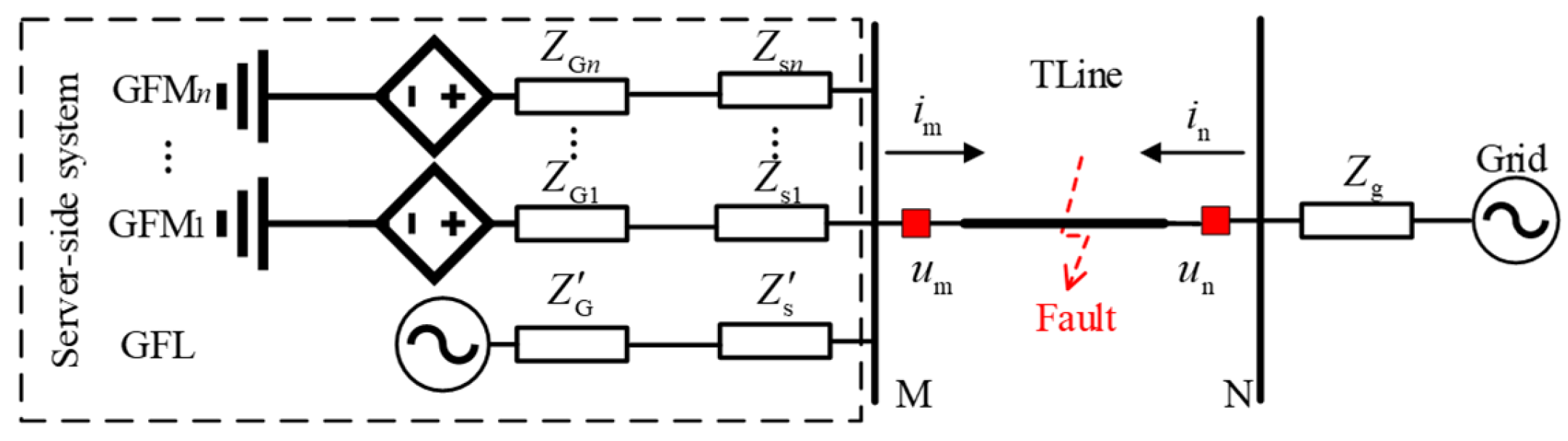
Figure 3 shows simplified transmission-line diagrams of a large-scale power system under normal operation and under an internal fault. Taking line MN as an example, the voltages and currents at the two terminals are coupled through relationships determined by the line parameters. Let the instantaneous voltages and currents at terminals M and N be denoted by u_m, u_n, i_m, and i_n, respectively. Taking the single-phase π-type line as an example, the total parameters of the line are R, L, and C, and the parallel conductance is not considered. It is stipulated that i_m(t) and i_n (t) are both positive when they flow into the protected line. Then, the current flowing through the parallel capacitor at both ends is [22]

$$\left\{\begin{array}{l}{i}_{C\mathrm{m}}\left(t\right)={\displaystyle \frac{C}{2}}{\displaystyle \frac{\mathrm{d}{u}_{\mathrm{m}}\left(t\right)}{\mathrm{d}t}}\\ i_{C\mathrm{n}}\left(t\right)={\displaystyle \frac{C}{2}}{\displaystyle \frac{\mathrm{d}{u}_{\mathrm{n}}\left(t\right)}{\mathrm{d}t}}\end{array}\right.$$

(5)

The current of the branch connected in series on the circuit is

$$i_s\left(t\right)=i_{\mathrm{m}}\left(t\right)-{\displaystyle \frac{C}{2}}{\displaystyle \frac{\mathrm{d}{u}_{\mathrm{m}}\left(t\right)}{\mathrm{d}t}}$$

(6)

During normal operation or external faults, there are no additional faulty branches within the line; therefore,

$$i_{\mathrm{m}}\left(t\right)+i_{\mathrm{n}}\left(t\right)={\displaystyle \frac{C}{2}}\left[{\displaystyle \frac{\mathrm{d}{u}_{\mathrm{m}}\left(t\right)}{\mathrm{d}t}}+{\displaystyle \frac{\mathrm{d}{u}_{\mathrm{n}}\left(t\right)}{\mathrm{d}t}}\right]$$

(7)

According to the KVL equation of the series branch

$$u_{\mathrm{m}}\left(t\right)-u_{\mathrm{n}}\left(t\right)=R{i}_s\left(t\right)+L{\displaystyle \frac{\mathrm{d}{i}_{\mathrm{m}}\left(t\right)}{\mathrm{d}t}}$$

(8)

Substituting with i_s(t), we obtain a relationship that is entirely represented by instantaneous sampling values:

$$u_{\mathrm{m}}\left(t\right)-u_{\mathrm{n}}\left(t\right)=R{i}_{\mathrm{m}}\left(t\right)+L{\displaystyle \frac{\mathrm{d}{i}_{\mathrm{m}}\left(t\right)}{\mathrm{d}t}}-{\displaystyle \frac{RC}{2}}{\displaystyle \frac{\mathrm{d}{u}_{\mathrm{m}}\left(t\right)}{\mathrm{d}t}}-{\displaystyle \frac{LC}{2}}{\displaystyle \frac{{\mathrm{d}}^2{u}_{\mathrm{m}}\left(t\right)}{\mathrm{d}{t}^2}}$$

(9)

Therefore, under normal operating conditions, these quantities satisfy

$$\Delta u=u_{\mathrm{m}}-u_{\mathrm{n}}=f\left(i_{\mathrm{m}},i_{\mathrm{n}}\right)$$

(10)

The function f(.) is associated with line parameters such as line-to-ground capacitance. It describes the numerical relationship among u_m–u_n, i_m, and i_n during normal operation and external faults. Because this theoretical basis is mainly based on the voltage–current coupling characteristics at the terminal of the protected line, and is mainly related to the line parameters, its dependence on the short-circuit capacity at the source side is relatively low.

When a fault occurs within the dashed region in Figure 3, the fault branch changes the line structure and alters the coupling relationship among the electrical quantities. The terminal quantities then satisfy

$$\Delta u=u_{\mathrm{m}}-u_{\mathrm{n}}=g\left(i_{\mathrm{m}},i_{\mathrm{n}},i_f\right)$$

(11)

Here, if denotes the fault current, and g(.) depends on the line-to-ground capacitance, transition resistance, and fault location. Under this condition, the electrical quantities at the two line terminals no longer satisfy Equation (10).

In principle, a fault can be identified by testing whether the terminal electrical quantities satisfy Equation (10). However, obtaining f(.) requires equivalent line modeling, and fault identification based on f(.) requires iterative solution. These steps reduce protection speed and reliability. To avoid this difficulty, this paper constructs a three-dimensional curve from the voltages and currents at both line terminals. The problem of verifying Equation (10) is thereby transformed into a curve-shape matching problem for internal-fault identification.

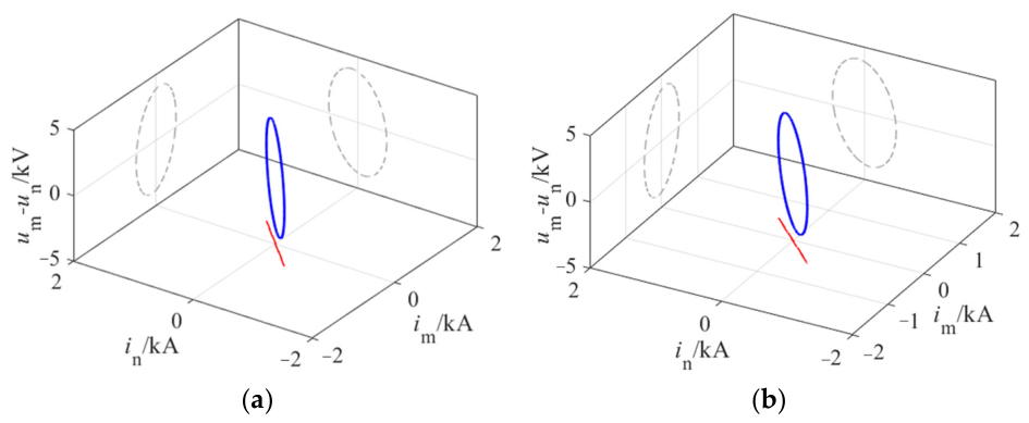
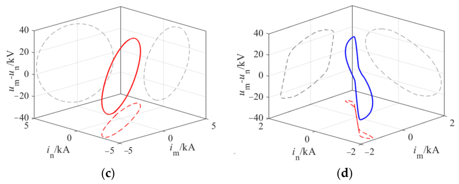
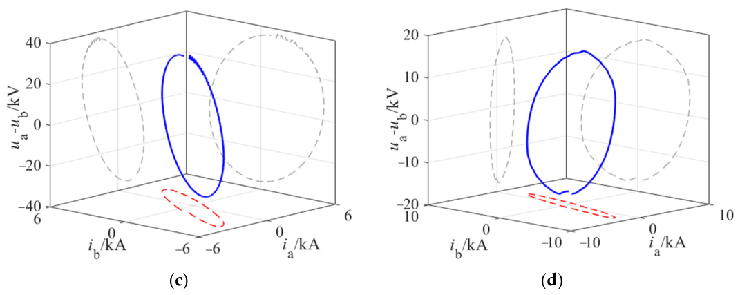
Figure 4 shows representative UICs and their projections under normal operation, internal faults, external faults, and external faults with CT saturation. During an internal fault, the line topology structure suddenly changes and fault current is injected, resulting in a decrease in voltage and an increase in current. At this time, the phase amplitudes of the currents at both ends are different, and under normal circumstances, the phase amplitudes of the voltages at both ends are also different. The resulting three-dimensional voltage–current curve is elliptical in shape and has a large area; however, during an external fault, the phase amplitudes of the currents and voltages at both ends are similar, and the curve still maintains an elliptical shape, but the area enclosed is significantly smaller. Therefore, these characteristics can be used to distinguish the curves of internal faults from those of external faults.

3.2. Curve Characteristic Analysis

The three-dimensional voltage–current ellipses associated with different operating and fault states differ substantially in geometric shape and spatial distribution. These states can therefore be distinguished using the ellipse area and its distribution in the three-dimensional coordinate system.

During normal operation, the voltages and currents at the two line terminals remain within the rated operating range, and i_m and i_n have similar magnitudes and nearly identical phases. During external faults, the currents on the two sides of the line also remain similar in magnitude and phase. The three-dimensional voltage–current curve constructed from these quantities therefore forms a small ellipse-like distribution concentrated near the y = x plane. CT saturation is usually limited under normal operating conditions [23]. When saturation occurs during an external fault, existing CT-saturation detection and correction methods are used to correct the UIC so that the curve retains the characteristics of an external fault [24].

During an internal fault, the fault branch changes the original line topology and introduces a large fault-current component. This produces a pronounced voltage sag on the line side and a clear difference between i_m and i_n. The area enclosed by the three-dimensional voltage–current ellipse increases significantly, and its spatial distribution deviates from the y = x plane.

The proposed three-dimensional voltage–current curve features therefore capture the variation patterns of terminal electrical quantities under different operating conditions. They support discrimination among internal faults, external faults, and normal operation while retaining clear physical meaning. Due to these characteristics being based on the voltage–current coupling at both ends of the line, their impact on the power supply is relatively small, and they provide a basis for the protection standards developed in the following text.

4. Protection Principle Based on UIC Features

4.1. Fault Feature Extraction

To transform the elliptical UIC features into quantitative metrics for fault identification, three core features are extracted from the three-dimensional voltage–current ellipse. The definition and calculation formula are derived based on the sampled data collected during the first half of the period after the failure occurs, in order to meet the requirement of rapid fault identification. However, considering the influence of the transient process at the source side after the fault occurs, the protection scheme studied in this paper starts to collect voltage and current data 10 milliseconds after the fault [11,25,26]. Let the total post-fault sampling sequence length be N. Using the valid half-cycle data, the number of samples is n = N/2. Since the collected current and voltage data are all instantaneous values, the peak values of the voltage and current under the rated operating condition are used as the reference values for normalization processing.

• Trajectory divergence

Trajectory divergence characterizes the overall dispersion of the three-dimensional voltage–current trajectory and reflects the spatial distribution of fault components. It is calculated as follows:

$$\left\{\begin{array}{l}S=\sqrt{{\sigma }_{i_{\mathrm{m}}}^2+{\sigma }_{i_{\mathrm{n}}}^2+{\sigma }_{\Delta u}^2}\\ {\sigma }_x=\sqrt{{\displaystyle \frac{1}{n-1}}{\displaystyle \sum _{k=1}^n{\left(x_k-\overline{x}\right)}^2}}\end{array}\right.$$

(12)

In Equation (12), σ_im, σ_in, and σ_Δu denote the standard deviations of the current and voltage difference sequences at terminals M and N, respectively. The arithmetic mean of sequence x_k is used in the standard deviation calculation. This feature has inherent disturbance resistance and requires no additional processing. For internal faults, the fault branch causes strong spatial dispersion and severe component fluctuations, so S is large. For external faults and normal operation, the terminal currents and voltages are more balanced, the fault-component fluctuations are milder, and the spatial distribution is concentrated, so S is small.

2.

Average distance from the sampling points to the plane y = x

The average distance from the sampling points to the plane y = x characterizes the perpendicular distance from the current vector to the symmetry plane i_m = i_n. It therefore reflects the degree of asymmetry between the terminal currents. To improve disturbance immunity, the two largest outliers are discarded before averaging. The instantaneous distance and the disturbance-resistant average distance are calculated as follows:

$$\left\{\begin{array}{l}{d}_{x=y,k}={\displaystyle \frac{\left|i_{\mathrm{m},k}-i_{\mathrm{n},k}\right|}{\sqrt{2}}}\\ D_{x=y}={\displaystyle \frac{1}{n-2}}{\displaystyle \sum _{k=1}^{n-2}sort\left(d_{x=y,k}\right)}\end{array}\right.$$

(13)

In Equation (13), sort d_x=y,k denotes the instantaneous distance sequence sorted in ascending order. The two largest outliers are removed, and the arithmetic mean is calculated from the remaining n − 2 samples. During an internal fault, the amplitudes and phases of the terminal currents differ markedly. The sampling points move away from the i_m = i_n symmetry plane, giving a large D_x=y value. During external faults and normal operation, the terminal currents remain highly similar and the sampling points stay close to the i_m = i_n plane, so D_x=y is small.

3.

Average spatial distance

The average spatial distance is defined as the mean Euclidean distance from the three-dimensional voltage–current vectors to the origin. It reflects the overall magnitude of the fault components. The same robustness treatment, removing the two largest outliers, is applied. The instantaneous spatial distance and the robust average distance are calculated as follows:

$$\left\{\begin{array}{l}{d}_k=\sqrt{i_{\mathrm{m},k}^2+i_{\mathrm{n},k}^2+\Delta u_k^2}\\ D_{avg}={\displaystyle \frac{1}{n-2}}{\displaystyle \sum _{k=1}^{n-2}sort\left(d_k\right)}\end{array}\right.$$

(14)

In Equation (14), sort d_k denotes the instantaneous spatial distance sequence sorted in ascending order. The two largest outliers are removed, and the arithmetic mean is calculated from the remaining n–2 samples. For internal faults, the fault current and differential voltage generated at the fault point have large amplitudes, so the three-dimensional vector is generally far from the origin. For external faults, the fault-component amplitudes are smaller, and the vector remains closer to the origin. This feature therefore distinguishes the strength of fault components intuitively.

The proposed method uses the first half-cycle of post-fault data. For the 50 Hz system and a sampling frequency of 20 kHz, the feature-extraction window is 10 ms and contains 200 samples. The computational efficiency was evaluated in MATLAB R2024a on a computer equipped with an Intel Core i7-14700KF processor and 32 GB RAM. The calculation of the three features in Equations (12)–(14) was repeated 80 times after program warm-up. The measured mean, median, and 95th-percentile computation times were 0.00629, 0.005959, and 0.007958 ms, respectively. Therefore, excluding protection-startup, communication, and circuit-breaker delays, the proposed criterion produced a classification result approximately 10 + 0.00629 ms after fault inception.

The three features are fused to construct the fault feature vector F = [S, D_x=y, D_avg]^T. This vector describes the difference between internal and external faults in terms of spatial dispersion, current similarity, and fault-component magnitude. Although CT-saturation correction is applied to the terminal currents to reduce waveform distortion, residual correction errors may remain. The complementarity of the three features improves the adaptability and robustness of the method under abnormal operating conditions.

4.2. Protection Criterion

After the three feature quantities are fused into F = [S, D_x=y, D_avg]^T, an ellipsoidal envelope based on second-order sample statistics is used to construct the feature space [27,28]. This feature space converts the quantitative UIC features into a criterion space for fault diagnosis. It is established from the statistical distributions of normal operation and external faults, whose feature patterns are stable. Internal faults are identified by calculating the distance between the online feature vector F and the ellipsoidal feature space.

• Offline feature-space construction

Eigenvalue decomposition of the covariance matrix is used to determine the principal directions of the ellipsoid. The second-order sample statistics, represented by the covariance, characterize the variability of the data along different directions. Let the sample points used for feature-space construction be p_i (i = 1, …, N). The covariance distance from the sample center μ can then be calculated using Equation (10), and the ellipsoidal feature-space center can be determined.

$$\left\{\begin{array}{l}\mu ={\displaystyle \frac{1}{N}}{\displaystyle \sum _{i=1}^N{p}_i}\\ \Sigma ={\displaystyle \frac{1}{N-1}}{\displaystyle \sum _{i=1}^N\left(p_i-\mu \right){\left(p_i-\mu \right)}^T}\end{array}\right.$$

(15)

The sample points are projected onto the principal-axis coordinate system so that the data extension can be represented by axial scales in the local coordinate system. The transformed sample point $p_i^{\prime }$ is expressed as

$$\left\{\begin{array}{l}{p}_i^{\prime }=R^T\left(p_i-\mu \right)\\ \mathsf{\Sigma }=R\Lambda R^T\end{array}\right.$$

(16)

In this equation, R is an orthogonal matrix whose columns are the eigenvectors of Σ. It defines the rotation from the original coordinate system to the principal-axis coordinate system.

A rotating ellipsoid is then constructed in the principal-axis coordinate system. Equal radii a and b are assigned to the first and second principal axes, and radius c is assigned to the third principal axis. The analytical form of the ellipsoid in the local coordinate system is given by Equation (17).

$${\displaystyle \frac{x^2+y^2}{a^2}}+{\displaystyle \frac{z^2}{c^2}}\le 1$$

(17)

To include the samples, a, b, and c are solved using Equation (18). For points that still lie outside the ellipsoid, the corresponding semi-axis is scaled proportionally until all points are enclosed. This process yields the major and minor axes that define the ellipsoidal feature space.

$$\left\{\begin{array}{l}a=b=\max \sqrt{x_i^{\prime 2}+y_i^{\prime 2}}\\ c=\max \left|z_i^{\prime 2}\right|\end{array}\right.$$

(18)

Here, x′, y′, and z′ are the components of p′. Thus, the feature space of normal operation and external faults is described by the ellipsoid center and by the major and minor axes calculated from Equations (15)–(18).

2.

Online fault detection criterion

In online applications, the UIC feature vector is calculated from the voltage and current data collected at both line terminals using Equations (12)–(14). The values of S, D_x=y, and D_avg in F are then substituted into x′, y′, and z′ in Equation (19) to calculate dF.

The value dF is the normalized distance from F to the ellipsoidal feature space. Equation (20) determines whether the sample lies inside or outside the ellipsoid. When dF > 1.0, the point lies outside the ellipsoid and is theoretically classified as an internal fault. When dF < 1.0, the point lies inside the ellipsoid and is classified as an external fault or normal operation. To account for transient effects during feature extraction, a reliability threshold of 1.1 is used in practical applications. If dF > 1.1, the condition is judged as an internal fault and the protection trips. Otherwise, it is judged as an external fault or normal operation, and line protection is blocked.

$$dF={\displaystyle \frac{x^{\prime 2}+y^{\prime 2}}{a^2}}+{\displaystyle \frac{z^{\prime 2}}{c^2}}$$

(19)

$$dF={\displaystyle \frac{x^{\prime 2}+y^{\prime 2}}{a^2}}+{\displaystyle \frac{z^{\prime 2}}{c^2}}\ge d_{\mathrm{set}}$$

(20)

The features of external faults on system-fed lines differ from those under normal operation. The discrepancy in electrical parameters becomes more pronounced as transition resistance increases and the fault location approaches the protected line. Therefore, low-resistance near-zone faults and selected far-zone faults are simulated to characterize the external-fault feature space. If normal-operation and external-fault samples are used to construct two separate subspaces, their sample distributions become more compact, which can further improve discrimination.

4.3. Protection Scheme

To satisfy the speed and reliability requirements of line protection, a startup criterion based on transient local voltage variations is established. This criterion uses only locally measured voltage data and identifies the initial fault disturbance by comparing changes in the fault-voltage component. The startup condition is expressed as

$$\Delta u\left(t\right)=\left|u\left(t\right)-u\left(t-T\right)\right|$$

(21)

Here, T denotes one power-frequency cycle, and u denotes the voltage at terminal M or N. When Δu(t) at either terminal exceeds the activation threshold Δu_set, a line fault is suspected. A high-frequency signal is then sent to activate protection at the local and remote terminals, and the fault feature vector is extracted from the UIC.

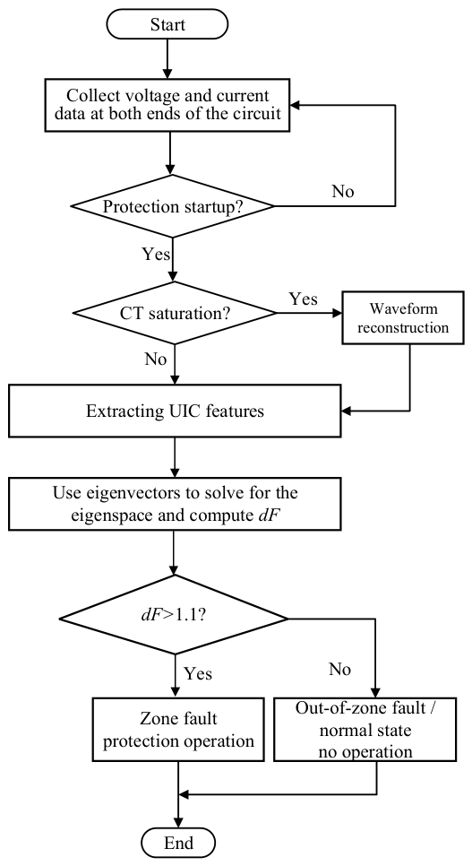
After line protection is activated, the terminal currents are checked for CT saturation. If saturation is detected, the measured currents are corrected [29].

Finally, Equation (20) is used to determine the position of the fault feature vector relative to the ellipsoid. When the internal-fault criterion is satisfied, a trip signal is issued.

The complete algorithmic flow of the proposed protection scheme is shown in Figure 5.

5. Results

To verify the preceding analysis and the proposed protection principle, we referred to the relevant opinions in reference [4] and constructed a 110 kV tie-grid-type power grid connection system, as shown in Figure 6 [30]. The 5 MW IIDG connected to bus N operates under a virtual synchronous generator (VSG) control scheme. An inertia time constant of 1 s and a damping coefficient of 0.002 p.u. are adopted, while the active- and reactive-power droop coefficients are set to 20 and 10, respectively. The model further incorporates low-voltage ride-through and current-limiting functions, and the converter output current is limited to 3.67 p.u. during faults. The photovoltaic source has a total capacity of 100 MW. The 0.38 kV/35 kV step-up transformer has a capacity of 120 MVA and a leakage reactance of 0.0676 pu. The busbar length is 200 m, with positive-sequence impedance Z₁ = 0.33 + j0.41 Ω/km, positive-sequence capacitive reactance to ground X_C1 = −j4.5473 × 10⁵ Ω·km, zero-sequence impedance Z₀ = 1.04 + j1.25 Ω/km, and zero-sequence capacitive reactance to ground X₀ = −j7.9577 × 10⁵ Ω·km. The local load consumes 15 MW active power and 1.5 Mvar reactive power. The 35 kV/110 kV step-up transformer has a capacity of 150 MVA, and its positive-sequence leakage reactance is 0.1 pu. The ab interconnection line is 20 km long, with positive-sequence impedance Z₁ = 0.01 + j0.41 Ω/km, positive-sequence capacitance-to-ground reactance X^′_C1 = −j3.5886 × 10⁸ Ω·km, zero-sequence impedance Z₀ = 0.33 + j1.32 Ω/km, and zero-sequence capacitance-to-ground reactance X^′_C0 = −j5.1175 × 10⁸ Ω·km. The grid-side equivalent impedance is Z_g = 0.020 + j14.137 Ω, and the grid source is modeled as an ideal 110 kV voltage source.

In the simulation model, a line fault is applied at 1 s. After fault inception, voltage and current data are collected from both line terminals, and the proposed criterion is used to protect line ab. The sampling frequency of the simulated voltage and current signals is 20 kHz.

5.1. Feature-Space Modeling

Because feature variations are relatively stable under normal operation and external faults, and because the fault features show strong clustering, a feature space can be constructed from normal-operation and external-fault samples. This space provides the basis for discriminating internal and external faults. Using the three-dimensional feature vector F = [S, D_x=y, D_avg]^T, the simulation samples are statistically analyzed and represented by an ellipsoidal envelope in three-dimensional feature space.

The sample set includes several external-fault conditions: single-phase-to-ground faults, phase-to-phase faults, phase-to-phase-to-ground faults, three-phase-to-ground faults, and three-phase faults. The transition resistance is varied from 50 Ω to 200 Ω, and 30 dB noise is superimposed to improve the adaptability of the feature-space construction to complex operating environments. The PCA-based rotating ellipsoid method described above is then used to determine the center, principal-axis directions, and semi-axis lengths of the feature space.

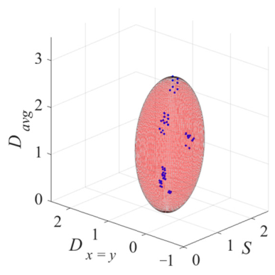
To construct the ellipsoidal feature space, 80 external-fault cases under different operating conditions were selected as the training samples. These cases include representative and extreme scenarios, such as metallic grounding faults at the protected line end and external faults with 30 dB noise. The ellipsoidal feature space is then obtained from the second-order sample moments of the selected dF values, which determine the center, principal-axis directions, and semi-axis lengths of the ellipsoid. This construction ensures that the selected external-fault samples are enclosed within the ellipsoidal feature region. The resulting ellipsoidal feature space for external faults and normal operation is shown in Figure 7. As can be seen from the graph, the values of the external fault samples are lower than 1.1, while the values of the internal fault samples are significantly higher than 1.1.

The ellipsoid center is μ = [0.7687, 0.0518, 1.6535], with semi-axes a = b = 0.6844 and c = 1.3889. The normal operation and external-fault samples are mainly distributed within or near this ellipsoidal feature space, indicating that the constructed space captures the statistical distribution of external operating conditions.

This feature space defines the discrimination criterion. If the feature vector of a test sample lies within the ellipsoidal space, namely dF < 1.1, the condition is classified as an external fault or normal operation. If the feature vector exceeds the feature-space boundary, namely dF > 1.1, the condition is classified as an internal fault.

5.2. Performance of the Protection Criterion

It should be noted that a total of 150 cases were generated, including 40 internal faults, 100 external faults, and 10 normal operating cases. The training and test subsets contain 100 and 50 cases, respectively. The training subset, containing only normal-operation and external-fault cases, was used to estimate the mean vector and covariance matrix of the ellipsoid. Internal-fault samples were not used in fitting the external-fault feature space. The independent test subset was then used only once for final performance evaluation.

Using the ellipsoidal feature space, internal-fault samples under different fault locations, transition resistances, fault types, noise levels, and CT-saturation conditions were tested to evaluate the effectiveness and robustness of the proposed method.

• Effect of fault location

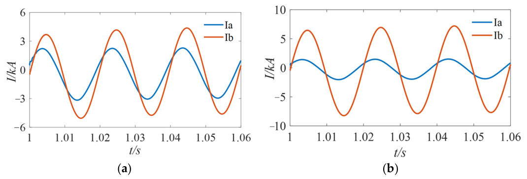
Single-phase-to-ground faults at different locations were simulated and compared. Figure 8 shows the UICs and current waveforms at both line terminals for a single-phase-to-ground fault inside the protected zone with a transition resistance of 50 Ω. The fault is located 2 km from end a and 2 km from end b. In both cases, the change in line topology causes the fault components to be affected by the fault branch. The components fluctuate substantially, and the currents at ends a and b differ markedly from those observed during external faults and normal operation.

Table 1. Fault-location identification results.

Fault Scenario	Fault Location (km)	dF	Classification
Internal	2/20	7.6928	Internal fault
Internal	5/20	8.4978	Internal fault
Internal	10/20	11.1279	Internal fault
Internal	18/20	21.6788	Internal fault

lists the identification results for single-phase-to-ground faults at different locations along the 20 km line (2, 5, 10, and 18 km from measurement point a), confirming the effectiveness of the proposed method.

2.

Effect of transition resistance

For ground faults,

Table 2. Identification results under different transition resistances.

Fault Scenario	Transition Resistance (Ω)	dF	Classification
Internal	0	11.1111	Internal fault
External	0	0.7486	External fault
Internal	10	11.1175	Internal fault
External	10	0.7488	External fault
Internal	100	11.1450	Internal fault
External	100	0.7494	External fault
Internal	300	11.2125	Internal fault
External	300	0.8630	External fault

lists the identification results for single-phase-to-ground faults at the midpoint of line ab with transition resistances of 0, 10, 100 and 300 Ω. In the event of an external fault, the fault location is set at a distance of 2 km from the b end of the protected line. As shown in the table, the size of the transition resistance has little impact on the calculation results of dF. Even at high transition resistance, the current difference between the two line terminals remains substantial for faults inside the protected zone, and the proposed line protection method remains effective.

3.

Effect of fault type

Although single-phase-to-ground faults are the most common transmission-line fault type, other fault types must also be considered.

Table 3. Discrimination results for different fault types.

Fault Scenario	Fault Type	dF	Classification
Internal	A-G	11.1279	Internal fault
External	A-G	0.7671	External fault
Internal	B-C	35.9846	Internal fault
External	B-C	0.9009	External fault
Internal	A-B-C	36.3677	Internal fault
External	A-B-C	0.2524	External fault
Internal	B-C-G	35.3029	Internal fault
External	B-C-G	0.2722	External fault
Internal	A-B-C-G	36.4202	Internal fault
External	A-B-C-G	0.2557	External fault

lists the identification results for single-phase-to-ground, phase-to-phase, three-phase, phase-to-phase-to-ground, and three-phase-to-ground faults at the midpoint of line ab, with a transition resistance of 50 Ω. In the event of an external fault, the fault location is set at a distance of 2 km from the b end of the protected line. Across these fault types, the voltage–current characteristic curves of the faulted phase at both line terminals retain the internal-fault features, and the proposed protection method remains effective.

4.

Noise disturbance

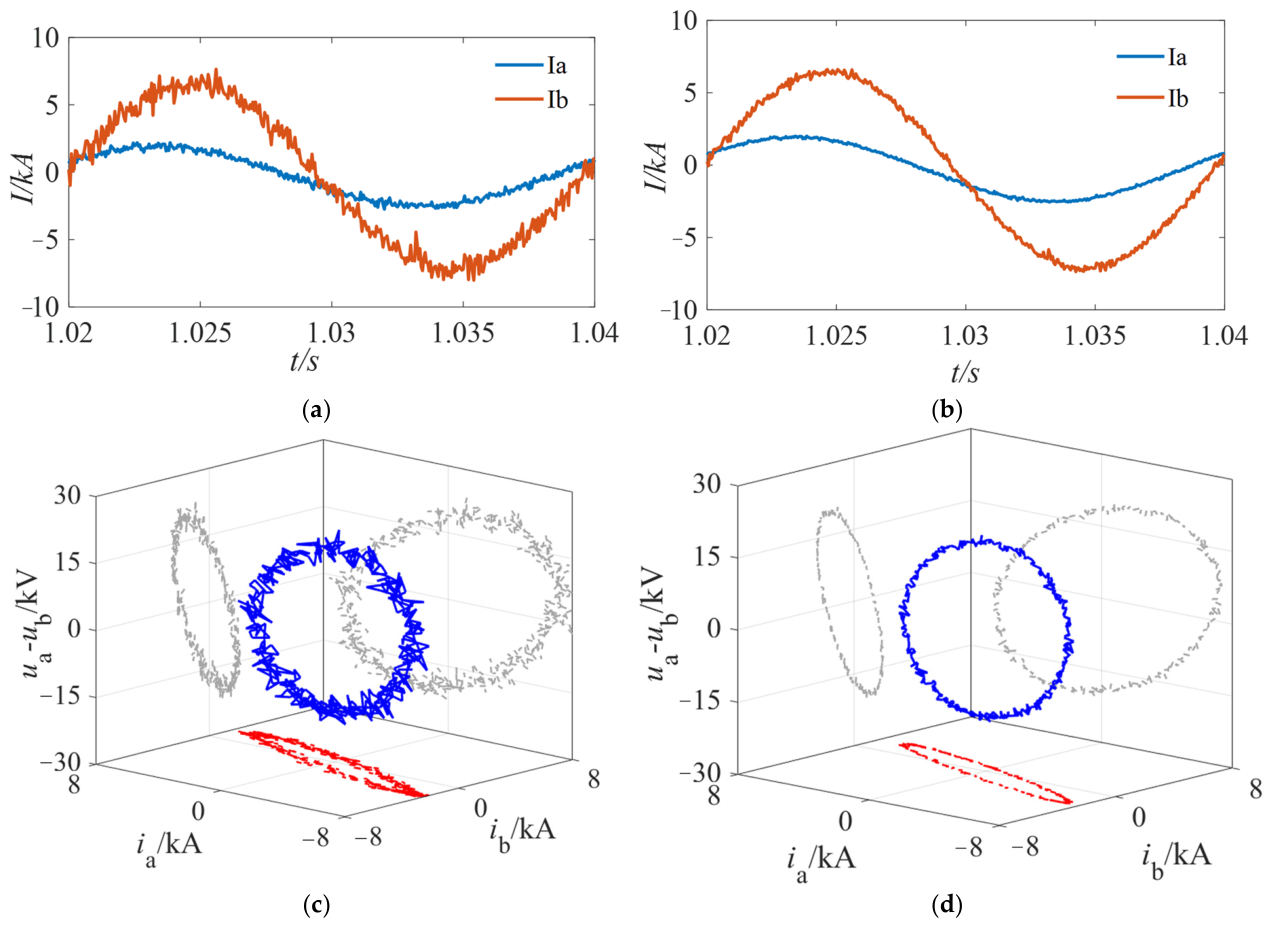
To evaluate robustness under practical operating conditions, a single-phase-to-ground fault at the midpoint of line ab was simulated with a transition resistance of 50 Ω and noise levels of 20 and 30 dB. Figure 9 shows the corresponding voltage and current response curves, and

Table 4. Discrimination results under noise disturbance.

Fault Scenario	Noise Level (dB)	dF	Classification
Internal	20	12.2144	Internal fault
External	20	0.8351	External fault
Internal	30	11.3542	Internal fault
External	30	0.7725	External fault

lists the identification results. In the event of an external fault, the fault location is set at a distance of 2 km from the b end of the protected line. The proposed protection scheme operates correctly under noisy conditions and shows good noise immunity.

If the noise level becomes sufficiently severe to affect the reliability of the protection decision, an appropriate filtering or denoising procedure may be incorporated before feature extraction. This limitation and the possible improvement have been clarified in the revised manuscript.

5.

CT saturation

To evaluate performance under CT saturation, an external single-phase-to-ground fault with a transition resistance of 50 Ω was simulated outside the protected zone. The rated transformation ratio of the CT was 1200/1 A, with a rated frequency of 50 Hz, an accuracy class of 5P20, a secondary winding resistance of 5 Ω, and a rated secondary burden of 15 VA. Since the rated secondary current was 1 A, the corresponding burden resistance was 15 Ω, resulting in a total secondary-loop resistance of 20 Ω. The knee-point voltage of the excitation characteristic was set to approximately 400 V. In the conventional saturation case, the primary fault current was 12 kA and the initial remanent flux was zero. The system X/R ratio was set to 20, corresponding to a decaying-DC time constant of approximately 63.7 ms at 50 Hz.

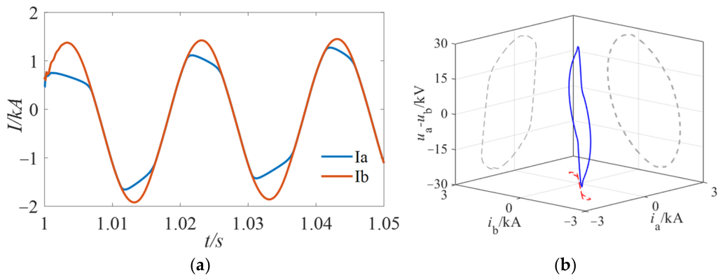
Figure 10 shows the voltage–current curve when slight CT saturation occurs on the a-side current transformer before correction.

Table 5. Discrimination results under CT-saturation scenarios.

Fault Scenario	Fault Type	Transition Resistance (Ω)	Noise Level (dB)	dF	Classification
External	A-G	50	0	0.7954	External fault
External	A-G	200	0	0.7395	External fault
External	A-B-C	50	0	0.3181	External fault
External	A-G	50	20	0.9047	External fault
External (after correction)	A-G	50	0	0.5443	External fault

lists the identification results under several CT-saturation conditions. In the event of an external fault, the fault location is set at a distance of 2 km from the b end of the protected line. As can be seen from the table, after the CT saturation occurs, regardless of whether the current data has been corrected or not, the method proposed in this paper can reliably identify the fault.

6.

Composite power supply

To investigate the adaptability of the proposed criterion to changes in source-side composition, an additional grid-following inverter-based source was connected in parallel with the original grid-forming source. The grid-following inverter adopts PLL-based synchronization and constant P-Q control. It further incorporates low-voltage ride-through and current-limiting functions, and the converter output current is limited to 1.1 p.u. during faults. The grid-forming and grid-following sources have rated capacities of 100 MVA. Thus, the source-side system represents a mixed grid-forming/grid-following configuration.

As shown in

Table 6. The calculation result of dF in the composite power supply scenario.

Fault Scenario	Fault Type	Fault Location (km)	Transition Resistance (Ω)	Noise Level (dB)	dF	Classification
External	A-G	-	0	0	0.06570	External fault
Internal	A-G	10/20	0	0	32.6509	Internal fault
External	B-C	-	100	0	0.9382	External fault
Internal	B-C	10/20	100	0	22.5996	Internal fault
External	A-B-C	-	0	0	0.5622	External fault
Internal	A-B-C	2/20	0	0	12.0170	Internal fault
External	B-C-G	-	300	0	0.4867	External fault
External	A-B-C-G	-	0	0	0.3451	External fault
External	B-C-G	-	0	20	0.4836	External fault
External	A-B-C-G	-	100	20	0.3411	External fault

, for the composite power supply scenario, the calculated dF values are obtained when different fault locations, transition resistances, and fault types occur. In the event of an external fault, the fault location is set at a distance of 2 km from the b end of the protected line. It can be seen that even if the power characteristics of the source side and the control strategy are changed, the method proposed in this paper is still applicable.

5.3. Method Comparison

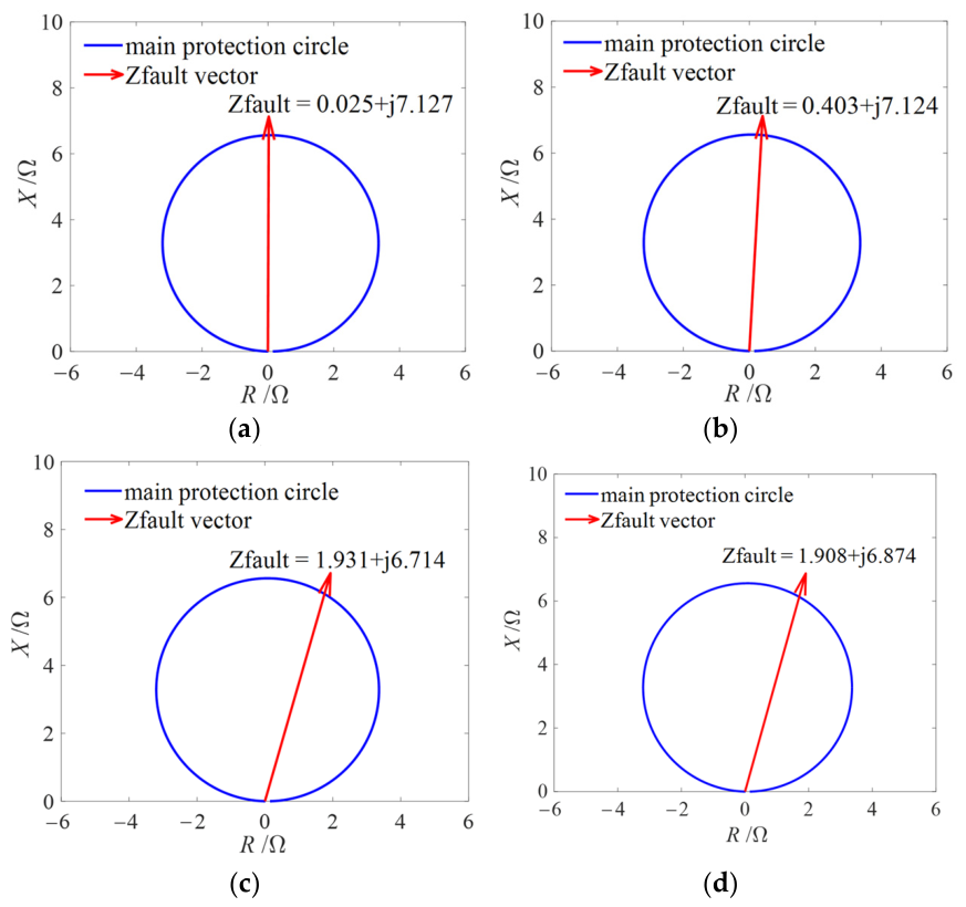
The conventional distance protection of line ab was tested using the simulation model in Figure 6 and standard distance-protection setting principles. Four simulation cases were selected: the fourth fault condition in Table 1, the seventh fault condition in Table 2, and the third and fifth fault conditions in Table 3. The results are shown in Figure 11. In all four cases, the measured impedance did not enter the setting range, so conventional distance protection failed to operate. This failure is caused by the low fault current and weak current-transfer characteristics of inverter-based power sources, together with the influence of control strategies.

In

Table 7. Comparison of recognition results between traditional distance protection and the method proposed in this paper under different scenarios.

Test Condition	Fault Type	Fault Location (km)	Transition Resistance (Ω)	Noise Level (dB)	Distance Protection	Proposed Method
Case 1	A-G	2/20	0	0	√	√
Case 2	A-G	5/20	50	0	√	√
Case 3	A-G	10/20	50	0	√	√
Case 4	A-G	18/20	50	0	×	√
Case 5	A-G	18/20	100	0	×	√
Case 6	A-G	18/20	0	0	×	√
Case 7	A-G	18/20	200	0	×	√
Case 8	B-C	10/20	50	0	√	√
Case 9	A-B-C	10/20	0	0	√	√
Case 10	B-C-G	10/20	50	0	√	√
Case 11	A-B-C-G	10/20	50	0	√	√
Case 12	B-C	18/20	50	0	×	√
Case 13	A-B-C	18/20	50	0	×	√
Case 14	A-G	10/20	0	20	√	√

, the discrimination results obtained by the two methods under several scenarios are presented. Compared with this, the fault protection scheme proposed in this paper is extremely accurate and reliable. In contrast, the identification accuracy rate of the traditional distance protection method is only 42.9%, and it is more prone to misjudgment.

Meanwhile, this method will also be compared with the parameter identification method [18] and the dual-end current protection method [31,32]. The fault condition is set as a single-phase grounding fault, the transition resistance is 0 Ω, and the fault location is 18/20 km. The calculation results are shown in

Table 8. Comparison of the identification results of various methods.

Method	Input	Complexity	Eigenvalue	Threshold	Correctness/Incorrectness
Proposed UIC	two-end u, i	O(nlogn)	11.1111	1.1	√
Parameter identification	one-end u, i	O[K(np2 + p3)]	19.999961 km	16.0000 km	×
Current-ratio method	two-end i	O(nlogn)	30.5788	25.0000	×
Kendall method	two-end u, i	O(n2)	0.9602	0	×

. From the perspective of computational complexity, this method is simpler and faster compared to the parameter identification methods, and it can correctly identify the fault under this condition.

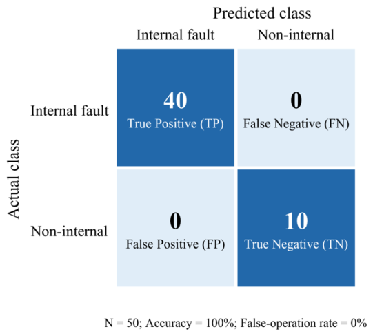
Additionally, 50 independent Monte Carlo test cases were evaluated. Taking an internal fault as the positive class, the test results were TP = 40, FN = 0, FP = 0, and TN = 10, as shown in Figure 12. The resulting dependability, security, sensitivity, false-operation rate, and overall accuracy were 100.0%, 100.0%, 100.0%, 0.0%, and 100.0%, respectively. Therefore, the proposed method is more suitable than conventional distance protection for grid-connection scenarios involving grid-forming inverters.

6. Conclusions

This paper proposes a transmission-line protection criterion based on voltage–current coupling features at both line terminals to address the reduced adaptability of conventional protection in systems with grid-forming renewable energy sources. The method constructs feature quantities from intrinsic line-side coupling relationships and uses multi-feature fusion to distinguish internal faults from external faults. PSCAD simulations show that the proposed scheme maintains reliable operation under different fault locations, transition resistances, fault types, noise levels, and CT-saturation conditions (including whether current reconstruction was applied). By comparison, the conventional distance-protection method achieved an accuracy of 42.9% in the considered cases. These results indicate that the proposed criterion is less sensitive to source-side short-circuit characteristics than the conventional impedance-based method because it relies on line-terminal voltage–current coupling features.

However, this conclusion is only applicable to the single system configuration and the hybrid grid-connected inverter model tested; for different inverter topologies, control strategies and current-limiting schemes, operating points, grid strength, and multi-inverter systems, further verification is still required. Additionally, the performance of this method under the condition of transformer excitation inrush current also needs to be further verified.

References

1. International Energy Agency. World Energy Outlook 2023; IEA: Paris, France, 2023. [Google Scholar]
2. Fan, Y.; Shao, X.; Muyeen, S.M.; Li, D.; Lin, S.; Chen, F. Disturbance observer based fractional-order integral sliding mode frequency control strategy for interconnected power system. IEEE Trans. Power Syst. 2021, 36, 5922–5932. [Google Scholar] [CrossRef] [Scilit]
3. Pulazza, G.; Zhang, N.; Kang, C.; Nucci, C.A. Transmission Planning with Battery-Based Energy Storage Transportation for Power Systems with High Penetration of Renewable Energy. IEEE Trans. Power Syst. 2021, 36, 4928–4940. [Google Scholar] [CrossRef] [Scilit]
4. Liang, Z.; Chung, C.Y.; Zhang, W.; Wang, Q.; Lin, W.; Wang, C. Enabling High-Efficiency Economic Dispatch of Hybrid AC/DC Networked Microgrids: Steady-State Convex Bi-Directional Converter Models. IEEE Trans. Smart Grid 2025, 16, 45–61. [Google Scholar] [CrossRef] [Scilit]
5. Wu, Y.; Liu, S.; Xu, R.; Hu, C.; Rui, T.; Feng, Z. Improved model-free predictive voltage control strategy for grid-forming inverters in weak grid with renewable energy sources. J. Power Electron. 2026. prepublish. [Google Scholar] [CrossRef] [Scilit]
6. Rizwan, M.; Gao, C.; Yan, X.; Ahmad, S.; Zaindin, M. An approach to disparage the blindness of backup protection in grid connected renewable energy sources system by inducing artificial fault current. Int. J. Electr. Power Energy Syst. 2023, 153, 109185. [Google Scholar] [CrossRef] [Scilit]
7. TQoria; Zhong, Q.-C.; Prevost, T.; Gruson, F. A PLL-free grid-forming control with decoupled functionalities for high-power transmission system applications. IEEE Access 2020, 8, 197363–197378. [Google Scholar] [CrossRef] [Scilit]
8. Yang, B.; Tang, J.; Guo, Y.; Zhao, L.; Li, Z.; Zhu, Y.; Zhang, X. An optimal fault restoration strategy of distribution networks considering the dynamic feature of distributed renewable energy resources. Energies 2026, 19, 1692. [Google Scholar] [CrossRef] [Scilit]
9. Maulà, G.; Savastio, L.P.; Amato, G.; Abdollahi, A.; De Tuglie, E.E. Characterization of disturbances induced by a microgrid on the distribution network. Sustain. Energy Grids Netw. 2025, 43, 101843. [Google Scholar] [CrossRef] [Scilit]
10. Cai, Y.; Qin, W.; Zhu, Z.; Lu, R.; Zhao, K.; Yan, Z. Active distance protection schemes for asymmetrical faults of renewable energy stations transmission line. Int. J. Electr. Power Energy Syst. 2026, 177, 111818. [Google Scholar] [CrossRef] [Scilit]
11. Taul, M.G.; Wang, X.; Davari, P.; Blaabjerg, F. Current limiting control with enhanced dynamics of grid-forming converters during fault conditions. IEEE J. Emerg. Sel. Top. Power Electron. 2020, 8, 1062–1073. [Google Scholar] [CrossRef] [Scilit]
12. Liu, Z.; Su, B.; Ji, Q.; Hu, Y. Local iterative calculation method and fault analysis of short-circuit current in high-voltage grid with large-scale new energy equipment integration. Sustainability 2024, 16, 11144. [Google Scholar] [CrossRef] [Scilit]
13. Liu, Z.; Yin, X.; Yin, X.; Lu, Q.; Qiao, J.; Wang, Y. A Dice similarity coefficient-based pilot protection method for 500 kV transmission lines of large-scale integrated photovoltaic power supply. Electr. Power Syst. Res. 2024, 226, 109918. [Google Scholar] [CrossRef] [Scilit]
14. Song, G.; Hou, J.; Guo, B.; Hussain, K.S.T.; Wang, T.; Masood, B. Active Injection for Single-Ended Protection in DC Grid Using Hybrid MMC. IEEE Trans. Power Deliv. 2021, 36, 1651–1662. [Google Scholar] [CrossRef] [Scilit]
15. Li, M.; Chen, K.; He, J.; Tang, Y.; Tang, J. Impedance Phase Based Active Injection Protection for Radial VSC-HVDC Grid. IEEE Trans. Power Deliv. 2023, 38, 1621–1635. [Google Scholar] [CrossRef] [Scilit]
16. Guo, Y.; Zhou, Z.; Li, M.; Wang, X.; Lv, P.; Yu, S. The line protection for outgoing lines of new energy power stations based on the equivalent parameter of line-to-ground admittance. IET Gener. Transm. Distrib. 2025, 19, e70053. [Google Scholar] [CrossRef] [Scilit]
17. Zheng, J.; Li, P.; Xu, K.; Kong, X.; Wang, C.; Lin, J.; Zhang, C. A distance protection scheme for HVDC transmission lines based on the steady-state parameter model. Int. J. Electr. Power Energy Syst. 2022, 136, 107658. [Google Scholar] [CrossRef] [Scilit]
18. Tu, Q.; Liu, W. Distance Protection for AC Transmission Lines of MMC-HVDC System With Offshore Wind Farms Based on Parameter Identification. In Proceedings of the 2022 4th International Conference on Smart Power & Internet Energy Systems (SPIES), Beijing, China, 27–30 October 2022; pp. 685–689. [Google Scholar]
19. Pattabiraman, D.; Lasseter, R.H.; Jahns, T.M. Transient Stability Modeling of Droop-Controlled Grid-Forming Inverters with Fault Current Limiting. In Proceedings of the 2020 IEEE Power & Energy Society General Meeting (PESGM), Montreal, QC, Canada, 2–6 August 2020; pp. 1–5. [Google Scholar]
20. Micallef, S.; Apap, M.; Cardoso, J.C.; Silva, G.M. Fault response of grid-forming converters: Current limiting and control interactions. IEEE Trans. Power Electron. 2021, 36, 10141–10154. [Google Scholar] [CrossRef] [Scilit]
21. Blackburn, J.L.; Domin, T.J. Protective Relaying: Principles and Applications, 4th ed.; CRC Press: Boca Raton, FL, USA, 2014. [Google Scholar]
22. Kang, X.; Suonan, J.; Song, G.; Bo, Z.Q. Protection technique based on parameter identification—Its principle and application. In Proceedings of the 2008 IEEE Power and Energy Society General Meeting, Pittsburgh, PA, USA, 20–24 July 2008; pp. 1–6. [Google Scholar]
23. Maulik, R.; Chothani, N.; Patel, D. Development of an adaptive differential protection scheme for transformer during current transformer saturation and over-fluxing condition. Int. Trans. Electr. Energy Syst. 2020, 31, e12751. [Google Scholar] [CrossRef] [Scilit]
24. Tajdinian, M.; Bagheri, A.; Allahbakhshi, M.; Seifi, A.R. Framework for current transformer saturation detection and waveform reconstruction. IET Gener. Transm. Distrib. 2018, 12, 3167–3176. [Google Scholar] [CrossRef] [Scilit]
25. Plet, C.A.; Graovac, M.; Green, T.C.; Iravani, R. Fault Response of Grid-Connected Inverter Dominated Networks. In Proceedings of the IEEE Power & Energy Society General Meeting, Minneapolis, MN, USA, 25–29 July 2010; pp. 1–8. [Google Scholar]
26. Bottrell, N.; Green, T.C. Comparison of Current-Limiting Strategies During Fault Ride-Through of Inverters to Prevent Latch-Up and Wind-Up. IEEE Trans. Power Electron. 2014, 29, 3786–3797. [Google Scholar] [CrossRef] [Scilit]
27. Wu, X.; Yan, J. A Second-Order Statistics-Based Mixed Sources Localization Method With Symmetric Sparse Arrays. IEEE Commun. Lett. 2020, 24, 1695–1699. [Google Scholar] [CrossRef] [Scilit]
28. Fang, Y.; Jia, K.; Yang, Z.; Li, Y.; Bi, T. Impact of inverter-interfaced renewable energy generators on distance protection and an improved scheme. IEEE Trans. Ind. Electron. 2019, 66, 7078–7088. [Google Scholar] [CrossRef] [Scilit]
29. ISantamaria; Scharf, L.L.; Ramírez, D. Scale-Invariant Subspace Detectors Based on First- and Second-Order Statistical Models. IEEE Trans. Signal Process. 2020, 68, 6432–6443. [Google Scholar] [CrossRef] [Scilit]
30. Mwongela, M.E.; Chang, C.-K. ANN based model for current transformers’ saturation error compensation in medium voltage switchgears. J. Electr. Eng. Technol. 2022, 17, 2171–2179. [Google Scholar] [CrossRef] [Scilit]
31. Zheng, B.; Chu, L.; Wang, Z. Transient protection principle based on current ratio of two terminals in frequency domain. Electronics 2022, 11, 1463. [Google Scholar] [CrossRef] [Scilit]
32. Li, L.; Sun, Y.; Zhao, Y.; Zhu, X.; Xiong, P.; Yang, W.; Hou, J. A fault direction discrimination method for a two-terminal weakly fed AC system using the time-domain fault model for the difference discrimination of composite electrical quantities. Electronics 2025, 14, 2556. [Google Scholar] [CrossRef] [Scilit]
Figure 1. Basic structure of a grid-forming power source.
Electronics 15 03923 g001
Figure 2. Equivalent model of a grid-forming power source.
Electronics 15 03923 g002
Figure 3. Simplified system schematic during normal operation and during an internal fault.
Electronics 15 03923 g003
Figure 4. UICs in different operating states. (a) Normal operation. (b) External fault. (c) Internal fault. (d) External fault with CT saturation.
Electronics 15 03923 g004aElectronics 15 03923 g004b
Figure 5. Flowchart of the proposed protection algorithm.
Electronics 15 03923 g005
Figure 6. Circuit topology used for simulation testing.
Electronics 15 03923 g006
Figure 7. Ellipsoidal feature region.
Electronics 15 03923 g007
Figure 8. Current waveforms and UICs for different fault locations. (a) Current waveform for a fault near terminal a. (b) Current waveform for a fault near terminal b. (c) UIC for a fault near terminal a. (d) UIC for a fault near terminal b.
Electronics 15 03923 g008aElectronics 15 03923 g008b
Figure 9. Current waveforms and UICs under noise disturbance. (a) Current waveform with 20 dB noise. (b) Current waveform with 30 dB noise. (c) UIC with 20 dB noise. (d) UIC with 30 dB noise.
Electronics 15 03923 g009
Figure 10. Voltage and current under CT-saturation conditions. (a) Current waveforms at both line terminals. (b) Voltage–current curve.
Electronics 15 03923 g010
Figure 11. Simulation results for conventional distance protection. (a) A-G, 18/20 km, 50 Ω. (b) A-G, 18/20 km, 200 Ω. (c) B-C, 18/20 km, 50 Ω. (d) A-B-C, 18/20 km, 50 Ω.
Electronics 15 03923 g011
Figure 12. Monte Carlo matrix.
Electronics 15 03923 g012