A Traceable Benchmarking Framework for Situation Assessment in Intelligent Flying Robotic Games

Abstract

Situation assessment (SA) supports maneuver decisions in dynamic three-dimensional robotic interactions, yet explicit methods depend on subjective factors and weights, whereas implicit learning-based methods are difficult to interpret. We propose a traceable benchmarking framework that standardizes motion dynamics, scenarios, capture-tagging rules, round-score metrics, and the decision carrier. Unified-Dimensional Situation Assessment (UDSA) converts heterogeneous advantages to a common altitude-equivalent scale, and Situation Assessment-Based Balanced Expert Decision-Making (SABED) enables controlled closed-loop comparison. Across five independent seeds, UDSA achieved mean round scores of 0.790 ± 0.010 against expert weighting and 0.710 ± 0.016 against Criteria Importance Through Intercriteria Correlation (CRITIC). Scenario-stratified, stress, and symmetric self-play summaries further supported robustness and label invariance. The released package enables reproduction of UDSA scoring, equivalence conversion, trajectory assessment, and the reported statistical summaries.

1. Introduction

Research on intelligent flying robots spans mobile-robot pursuit-evasion [1], reproducible single- and multi-agent learning environments [2,3,4,5], and autonomous drone racing [6,7]. Pursuit-evasion is a common benchmark for motion planning, interaction reasoning, and multi-agent decision-making. In these tasks, situation assessment (SA) summarizes an agent’s relative advantage and supports maneuver decisions.

In competitive aerial robotic games, relative speed, altitude, bearing angle, and distance jointly affect positioning, safety, and capture-tagging outcomes. SA is commonly organized around perception, comprehension, and projection [8]. Recent air-combat SA studies construct interpretable assessments through dynamic variable weighting, situation-knowledge extraction and weight optimization, or data-driven models for incomplete and weakly labeled information [9,10,11]. Objective weighting methods such as Criteria Importance Through Intercriteria Correlation (CRITIC) provide a transparent comparison baseline [12]. These methods remain sensitive to indicator design, task assumptions, and the scale on which heterogeneous factors are combined.

Implicit approaches learn nonlinear interactions through deep reinforcement learning and multi-agent reinforcement learning in robotic and competitive settings [13,14], including actor–critic formulations for mixed cooperative–competitive environments [15]. The value-based lineage includes Deep Q-Networks, Double DQN, and prioritized experience replay [16,17,18]; Rainbow and recurrent distributed replay provide subsequent combinations and extensions [19,20]. Recent aerial pursuit-evasion studies cover hierarchical control, high-speed evasion, online multi-UAV planning, opponent modeling, and cross-domain self-play [21,22,23,24,25]. Together with drone-racing results [6,7], these studies motivate traceable metrics, controlled baselines, and reproducible scenarios.

The unresolved gap is therefore a traceable method for mapping heterogeneous SA factors to a common closed-loop outcome while holding dynamics and decision logic fixed. The benchmark uses shared dynamics, scenarios, capture-tagging rules, round-score metrics, and one decision loop.

A prioritized experience replay double deep Q-network (PER-DDQN) is trained as the common discrete-maneuver module. The methodological contributions are outcome-equivalent factor conversion, UDSA, and controlled closed-loop SA comparison.

The main contributions of this paper are as follows:

(1)

The study environment was implemented with NetLogo 7.0.4 and its Python extension, enabling three-dimensional visualization, seeded batch evaluation, and direct calls to the UDSA module. The released package contains the tested Python bridge and UDSA runtime.

(2)

A benchmarking framework for situation assessment in intelligent flying robotic games is constructed. It reveals the influence of speed, altitude, and angular advantages on task outcomes through qualitative analysis, and realizes quantitative conversion among heterogeneous dominance factors using mean round score as the common criterion.

(3)

A Unified-Dimensional Situation Assessment method is proposed. The method converts speed and angular advantages into altitude-equivalent advantages according to their equivalent effects on mean round score, and then calculates the situation assessment value on a unified advantage scale, reducing the impact of subjective weight assignment.

(4)

A Situation Assessment-Based Balanced Expert Decision-Making method is proposed. Different assessment methods are embedded into the same SABED decision loop and evaluated by closed-loop mean round score, providing a unified objective benchmark for comparing SA methods.

Section 2 presents the simulation environment; Section 3 analyzes and converts speed, altitude, and angular advantages; Section 4 and Section 5 introduce UDSA and SABED; Section 6 reports experiments; Section 7 discusses limitations and future work; Section 8 concludes the paper; and Appendix A centralizes notation and the fitted surrogate coefficients.

2. Intelligent Flying Robotic Game Simulation Environment

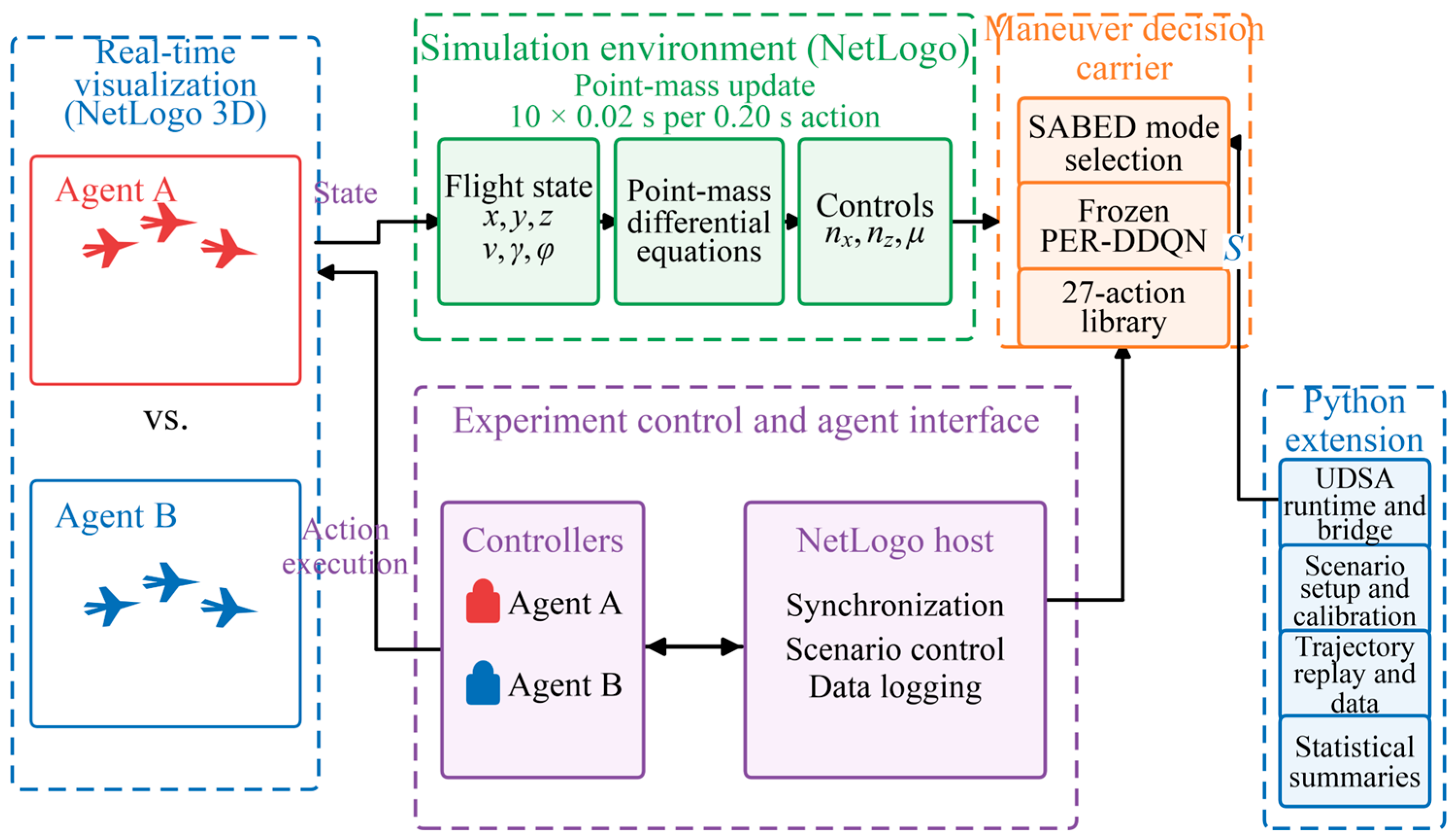
Figure 1 shows the framework implemented with NetLogo 7.0.4 and its Python extension [26]. The official NetLogo repository is the platform on which the framework is dependent. The accompanying package provides the UDSA source, Python-extension bridge, configuration, calibration tables, trajectory-replay utilities, and statistical summaries. NetLogo provides deterministic multi-agent execution, rapid reset, visualization, and direct Python integration, enabling larger controlled sweeps than higher-fidelity simulators such as AirSim or PyBullet [4,5]. This throughput advantage is obtained at the cost of aerodynamic and sensor fidelity; physical transfer requires higher-fidelity and hardware validation.

2.1. Aerial Robot Motion Model

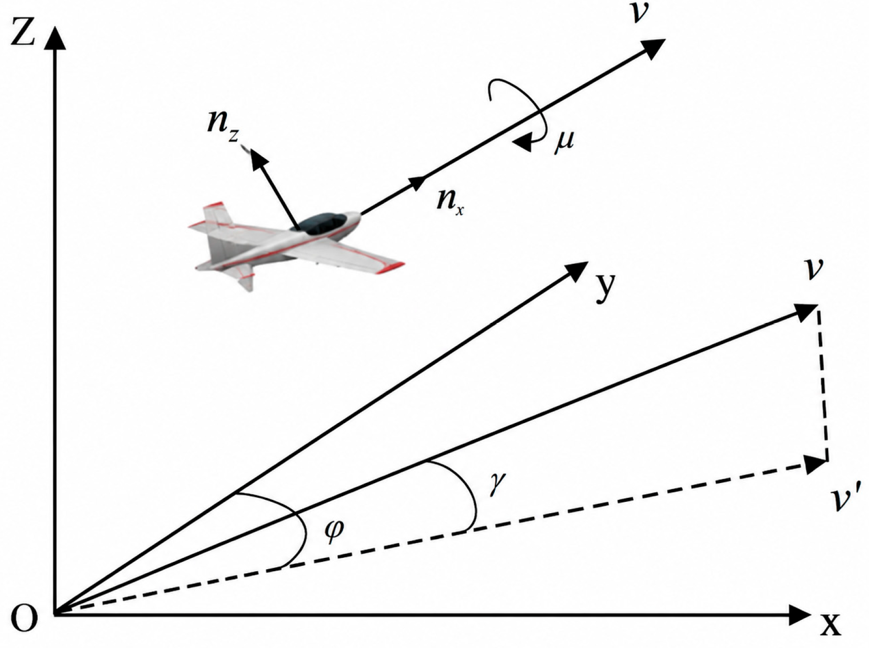
Figure 2 illustrates the six-state, three-dimensional point-mass fixed-wing reference model adopted from standard unmanned-aircraft practice [27]. The adopted formulation represents fixed-wing point-mass motion; rigid-body rotational dynamics are outside its six-state definition.

The state comprises three-dimensional position, speed magnitude, trajectory pitch, and trajectory yaw; the silhouette in Figure 2 adds no rigid-body states.

2.2. Aerial Robot Control Model

The model uses normalized tangential command n_x for acceleration, normalized vertical maneuver command n_z for climb or dive, and roll command μ for turning. Equation (1) maps these benchmark commands to the point-mass state update.

$$\left\{\begin{array}{l}{n}_x={\displaystyle \frac{\dot{v}}{g}}+\sin \gamma \hfill \\ n_z={\displaystyle \frac{1}{\cos \mu }}\cdot \left({\displaystyle \frac{v\dot{\gamma }}{g}}+\cos \gamma \right)\hfill \\ \mu =-{\displaystyle \frac{v\cos \gamma \dot{\phi }}{g{n}_z}}\hfill \end{array}\right.$$

(1)

where g is the acceleration of gravity, with a value of 9.8 m/s². The terms dφ/dt, dγ/dt, and dv/dt represent the rates of change of trajectory yaw angle, trajectory pitch angle, and speed, respectively.

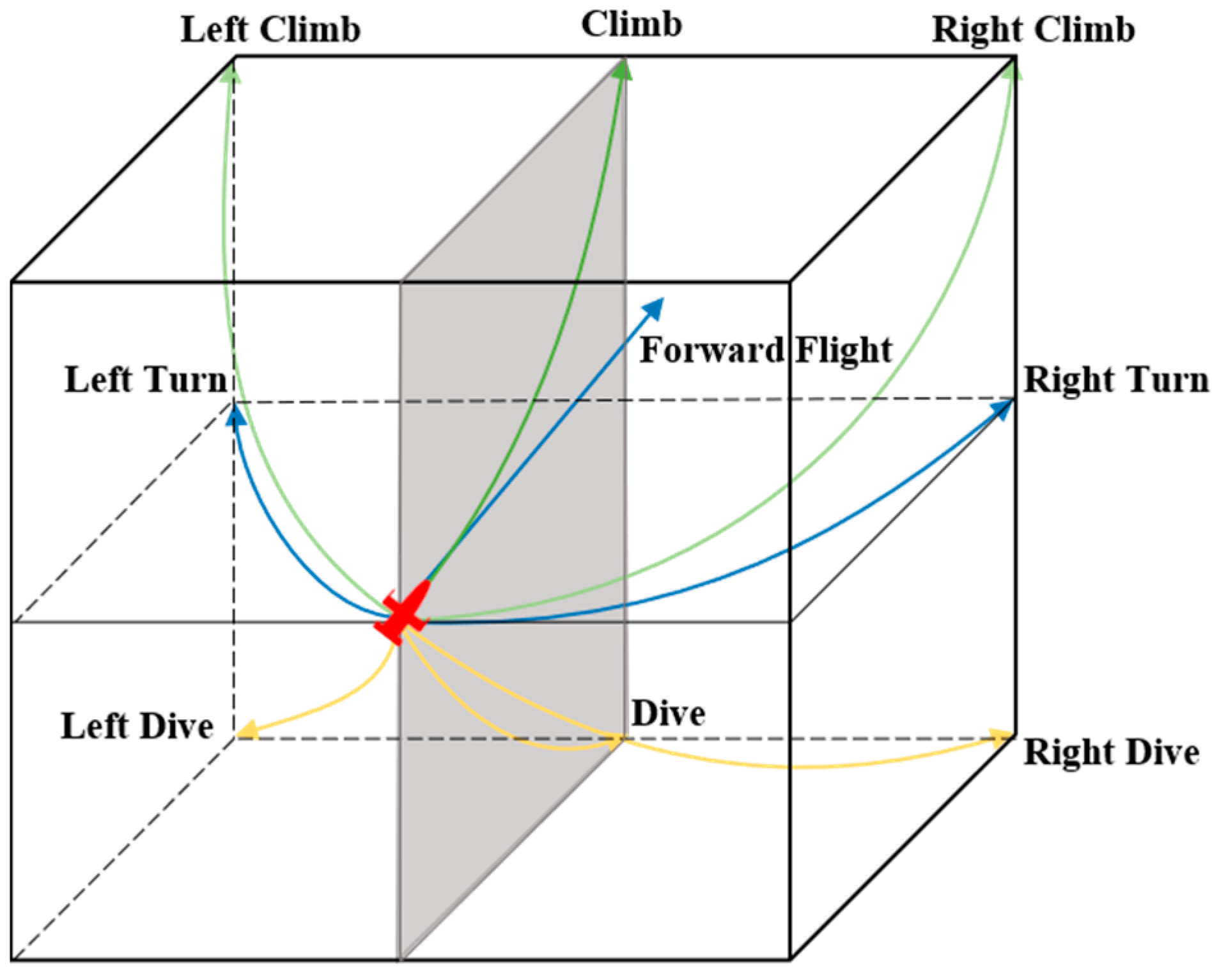
The benchmark specification combines the nine three-dimensional maneuvers in Figure 3 with acceleration, deceleration, and uniform-speed states, yielding 27 discrete actions. One action is held for a 0.20 s decision interval, corresponding to 10 integration steps at 0.02 s.

Table 1. Values of control parameters.

Control Parameter	Discrete Value
$n_x$	$\left\{-2,0,2\right\}$
$n_z$	$\left\{-8,1,2,5,8\right\}$
$\mu$	$\{-3\pi /4,-\pi /3,-\pi /4,0,\pi /4,\pi /3,3\pi /4\}$

lists the low-level command values used by the original simulator; the released package records the 0.20 s interval and 50 Hz replay rate.

The n_z values are dimensionless normal-maneuver commands used by the point-mass benchmark. The set {−8,1,2,5,8} retains the original simulator’s −8/+8 endpoint commands to provide clearly separated short-duration dive and climb responses while preserving the 27-action maneuver library used in all comparisons. Each command is held for 0.20 s, and the −8 command is limited to three consecutive selections. These values define the numerical benchmark envelope. For physical implementation, the command is saturated according to the certified normal-load and duration limits specified in the target platform’s flight manual.

2.3. Game Outcome Criteria

The capture-tagging task is a non-destructive interaction rule comparable to those used in robotic games and pursuit-evasion benchmarks. For agent i, a valid tag is the conjunction of an angular condition and a distance condition, as expressed in Equation (2):

$${\mathrm{tag}}_i=\mathbb{I}\left[\left({\theta }_i<{30}^{°}\right)\wedge \left({‖d‖}_2<d_{\mathrm{th}}\right)\right]$$

(2)

In Equation (2), a tag is valid only when the logical conjunction (θ_i < θ_th) ∧ (‖d‖₂ < dth) holds at the same integration step. The benchmark uses θ_th = 30 deg to define the counterpart agent’s rear interaction sector, and dth is the maximum valid tagging radius.

$$d_{th}=2000 \mathrm{m}+{v_i}^2/\left(10g\right)$$

(3)

In Equation (3), vi is the instantaneous speed of the tagging agent, clipped to the 100–500 m/s benchmark envelope before evaluating dth = 2000 m + v_i²/(10g). The divisor 10g serves as a numerical normalization in the tagging threshold. Structural loading requires a separate platform model. At 300 m/s, v_i²/(10g) = 918 m and dth is approximately 2.92 km; the threshold ranges from approximately 2.10 km at 100 m/s to 4.55 km at 500 m/s.

An agent succeeds by entering the counterpart’s rear sector within the tagging radius. A round is a draw if both agents meet the condition simultaneously or neither completes a valid tag before the simulation limit. Agent A receives a round score of 1 for a win, 0.5 for a draw, and 0 for a loss. Draws are retained in the denominator and are never discarded; thus, a ‘completed’ or ‘valid’ round includes wins, losses, and draws. The rule isolates relative angle and distance for objective comparison.

2.4. PER-DDQN Maneuver Decision-Making Algorithm

The benchmark adopts PER-DDQN as a common maneuver module. The five state components are the agent’s altitude, relative speed Δv, and separation d, and the two agents’ approach angles; every continuous component is linearly normalized to [−1, 1] using the training-envelope bounds. The 27 actions correspond to the maneuver library. A dueling architecture separates state value and action advantage, while residual connections stabilize feature extraction.

Table 2. Network and training configuration.

Parameter	Description	Value
Input Layer Neurons	State space dimension	5
Hidden Layer Structure	512 → 512 (residual) → 256 (dimensionality reduction) → 256 (residual)
Residual Block	Avoid gradient vanishing	2 × 512 − Dimensional + 2 × 256 − Dimensional
Dueling Structure	Value branch (256 → 1), advantage branch (256 → 27)
Activation Function	LeakyReLU
Target Network Update	Soft update	τ = 10−3
Loss Function	Huber loss
Optimizer	Parameter update	Adam
Learning Rate	Initial step size	1 × 10−4
Discount Factor	Future-return weight	γ = 0.99
Replay Buffer	Maximum stored transitions	200,000
Mini-Batch Size	Transitions per update	256
PER Priority Exponent	Sampling prioritization	α = 0.6
PER Importance Exponent	Bias correction schedule	β: 0.4 to 1.0
Exploration Rate	Linear decay over first 60% of training	ε: 1.0 to 0.05
Decision Interval	Action-hold duration	0.20 s
Training Episodes	Maximum episode count	5000
Replay Warm-Up	Transitions before learning	10,000

lists the network and training hyperparameters.

In the original experiments, a dueling residual network output Q-values for 27 actions. One policy was trained over randomized speed (100–500 m/s), altitude (5000–9000 m), and heading (0–360 deg) conditions and then frozen for every sweep and SA comparison; no condition-specific retraining was performed. The released package contains the five-seed training summary.

The shaped reward is r(t) = 0.4 clip[(d(t − 1) − d(t))/d₀, −1, 1] + 0.4[cos θ(t) − cos θ(t − 1)] − 0.001 + 10 I_win − 10 I_loss, where d₀ = 5000 m, I_win and I_loss are terminal indicators, and a draw has zero terminal bonus. The first two terms reward closing distance and improving the approach angle, the small time penalty discourages unnecessarily long episodes, and the terminal terms dominate the shaping terms.

The five seeded runs trained for at most 5000 episodes after a 10,000-transition warm-up. Convergence required less than 1% change in 200-episode return for five windows and less than 0.02 change on a fixed validation set. Across the five rows in PER_DDQN_training_summary.csv, the mean ± sample standard deviation was 3654 ± 160 episodes at convergence, 7.84 ± 0.23 for final return, 0.762 ± 0.019 for validation score, and 0.748 ± 0.021 for held-out test score.

3. Qualitative and Quantitative Analysis

With distance retained as the tag gate, the original controlled sweeps used Δv ∈ [−200, 200] m/s, Δh ∈ [−2000, 2000] m, and Δθ ∈ [−180, 180] deg. The released UDSA parameter and conversion tables cover the wider runtime domain Δv ∈ [−400, 400] m/s, Δh ∈ [−3000, 3000] m, and Δθ ∈ [−180, 180] deg; inputs outside this domain were clipped and are explicitly flagged.

3.1. Qualitative Analysis

3.1.1. Speed Advantage

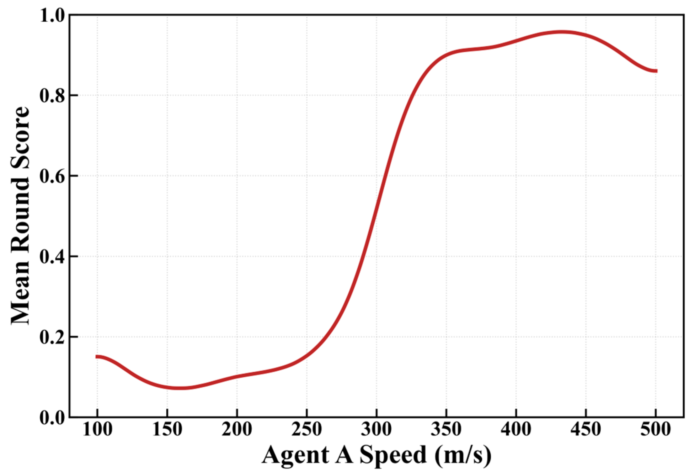
Figure 4 reports head-on and crossing sweeps with agent A at 100–500 m/s, agent B at 300 m/s, a 0.02 s step, and a 6000-step limit.

A win, draw, and loss score 1, 0.5, and 0, respectively; all outcomes remain in the denominator. The mean round score is defined by Equation (4), with 0.5 representing a neutral outcome under label symmetry:

$$mean round score = \left(W + 0.5D\right)/\left(W + D + L\right)$$

(4)

Figure 4 shows increasing score with speed advantage, with low-speed turning benefits and high-speed turning penalties producing small deviations from monotonicity.

3.1.2. Altitude Advantage

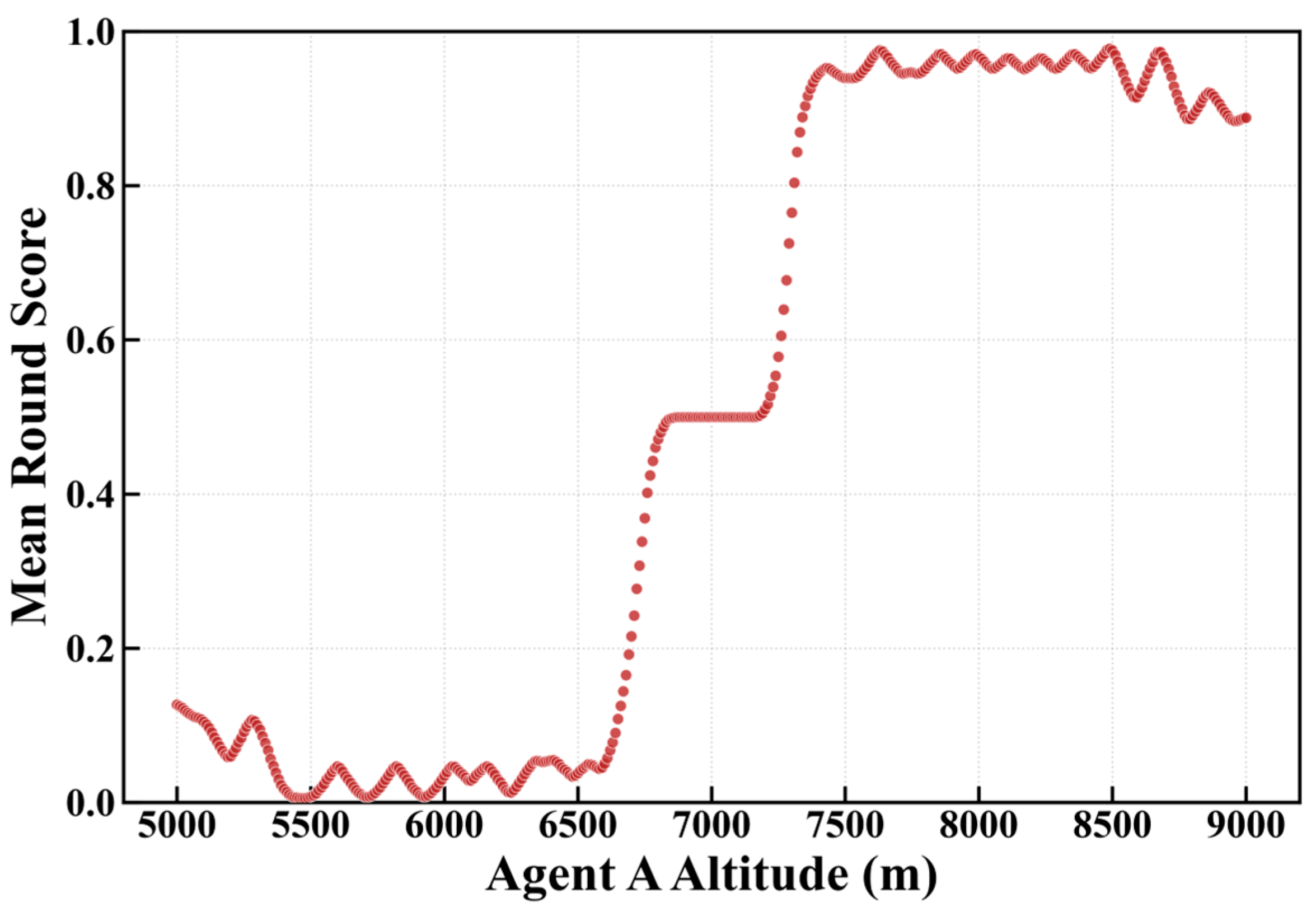
The altitude experiment uses the same head-on and crossing encounters. Agent A varies from 5000 to 9000 m, agent B remains at 7000 m, and both start at 200 m/s; all other settings follow Section 3.1.1. Figure 5 plots agent A’s mean round score against altitude.

Figure 5 shows a transition near equal altitude: higher altitude generally improves score, while very high altitude slightly degrades short-term positioning.

3.1.3. Angular Advantage

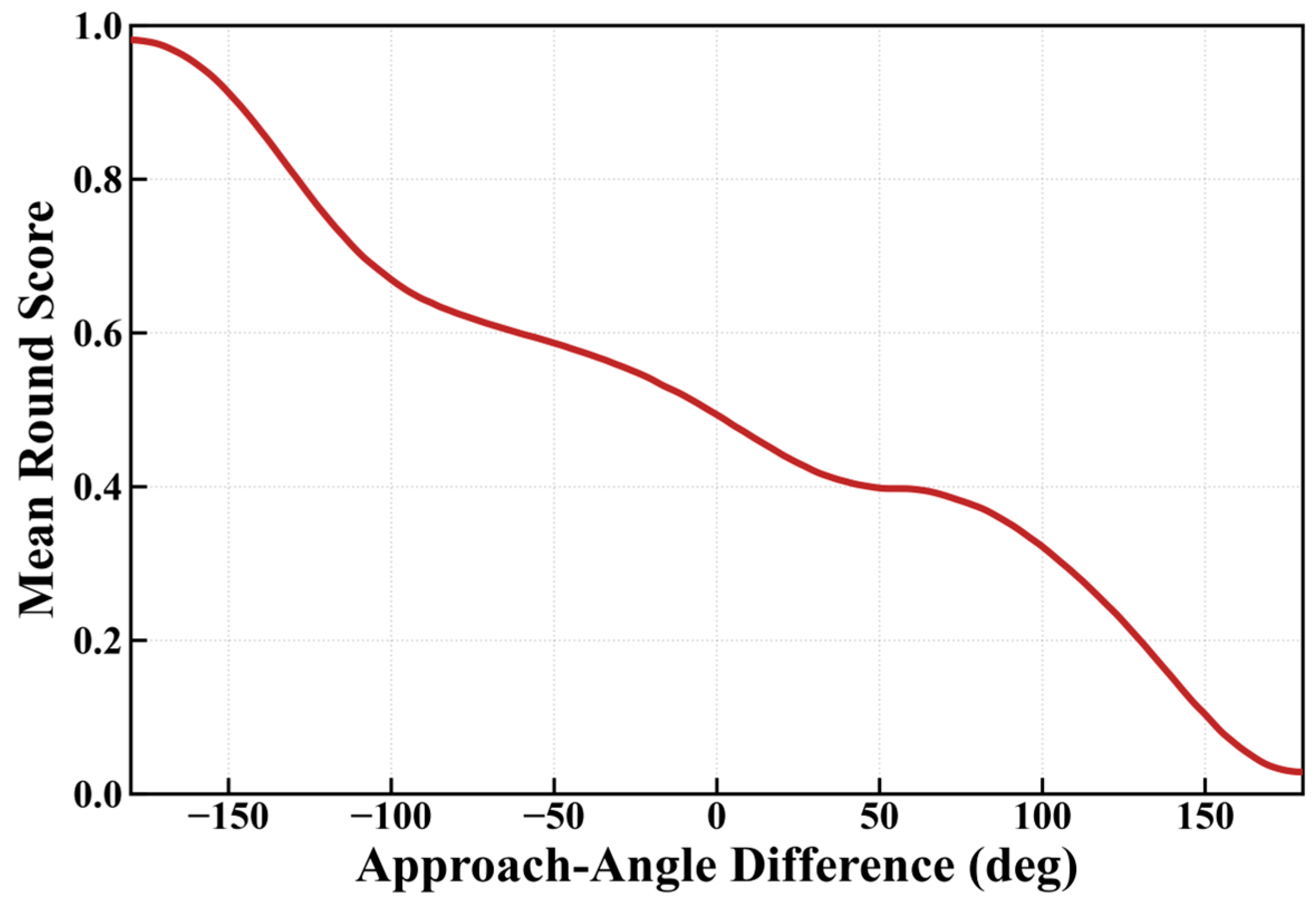
For angular advantage, both headings vary over [0 deg, 360 deg]. Agents A and B start at (1000, 2000, 7000) m and (1000, −2000, 7000) m, respectively, at 270 m/s. Figure 6 plots mean round score against the approach-angle difference Δθ = α_A − α_B.

Figure 6 shows high scores for rear approaches, approximately neutral scores near balanced headings, and low scores when agent A is exposed to the counterpart’s favorable sector.

3.2. Quantitative Analysis

Because heterogeneous dominance factors cannot be compared directly, mean round score is used to quantify conversion among speed, altitude, and angular advantages.

3.2.1. Conversion of Speed and Altitude Advantages

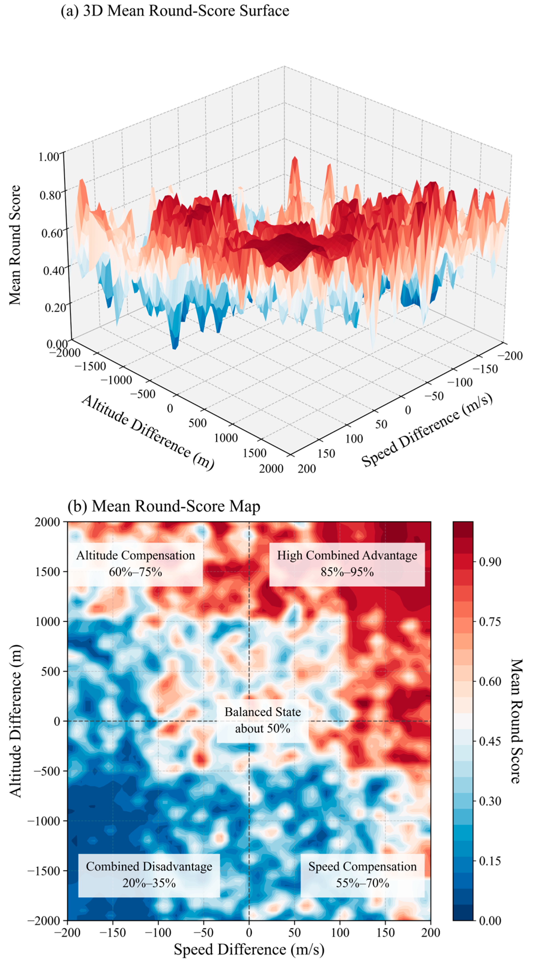
For the original speed–altitude sweep, agent A varied from 5000 to 9000 m while agent B remained at 7000 m and agent A stayed at 300 m/s while agent B varied from 100 to 500 m/s. Both used the frozen PER-DDQN policy described in Section 2.4. Figure 7 is retained as the reported sweep output.

Figure 7 presents a 3D surface and 2D heat map of agent A’s mean round score over speed and altitude differences, with red and blue indicating higher and lower mean round scores.

Figure 7 shows nonlinear compensation: altitude advantage can offset speed disadvantage, whereas being lower and slower yields low score.

The released speed–altitude surrogate uses x_v = Δv/150 and x_h = Δh/1150 and retains a sparse odd polynomial basis so that exchanging the two agents reverses the predicted advantage.

$$\Delta E=0.5\left({v_A}^2-{v_B}^2\right)+g\left(h_A-h_B\right)$$

(5)

$$c_e=tanh\left(\Delta E/\mathrm{100,000}\right)$$

(6)

The specific-energy difference ΔE = 0.5(v_A² − v_B²) + g(h_A − h_B), in J kg⁻¹, is retained as a diagnostic and as one CRITIC criterion in trajectory replay. The implemented CRITIC energy benefit is c_e = tanh(ΔE/100,000); UDSA itself uses only the signed differences Δv, Δh, and Δθ, preventing energy from double-counting speed and altitude. To capture the nonlinear relationship between the normalized advantage variables and the calibrated criterion, a polynomial feature mapping is introduced. Here, x denotes the normalized input vector composed of the signed advantage variables, and d represents the maximum polynomial order.

$$\varphi \left(x\right)=\left[1,x_1,x_2,\dots ,x_n,x_1^2,x_1{x}_2,\dots ,x_n^d\right]$$

(7)

The feature vectors of all calibration samples are stacked to form the ordered feature matrix X. The calibration targets are antisymmetrized as f_sym(x) = 0.5 + [f_raw(x) − f_raw(-x)]/2, which enforces f_sym(-x) = 1 − f_sym(x). The coefficient vector β is then obtained through ridge regularization, which provides a stable estimation of the fixed reference parameters with α = 10⁻³ and a sparse basis through the fifth order:

$$\underset{\beta }{\min }{\Vert y-X\beta \Vert }_2^2+\alpha {\Vert \beta \Vert }_2^2$$

(8)

In Equation (8), y denotes the calibration target, X the ordered feature matrix, β the coefficient vector, and α the ridge coefficient. The released basis, normalization constants, coefficients, equivalence tables, and p-hat = 0.5 boundaries are included in data/calibration. generate_calibration_tables.py reads the fixed parameter csv and regenerates the equivalence and boundary tables; it does not refit the coefficients.

3.2.2. Conversion of Speed and Angular Advantages

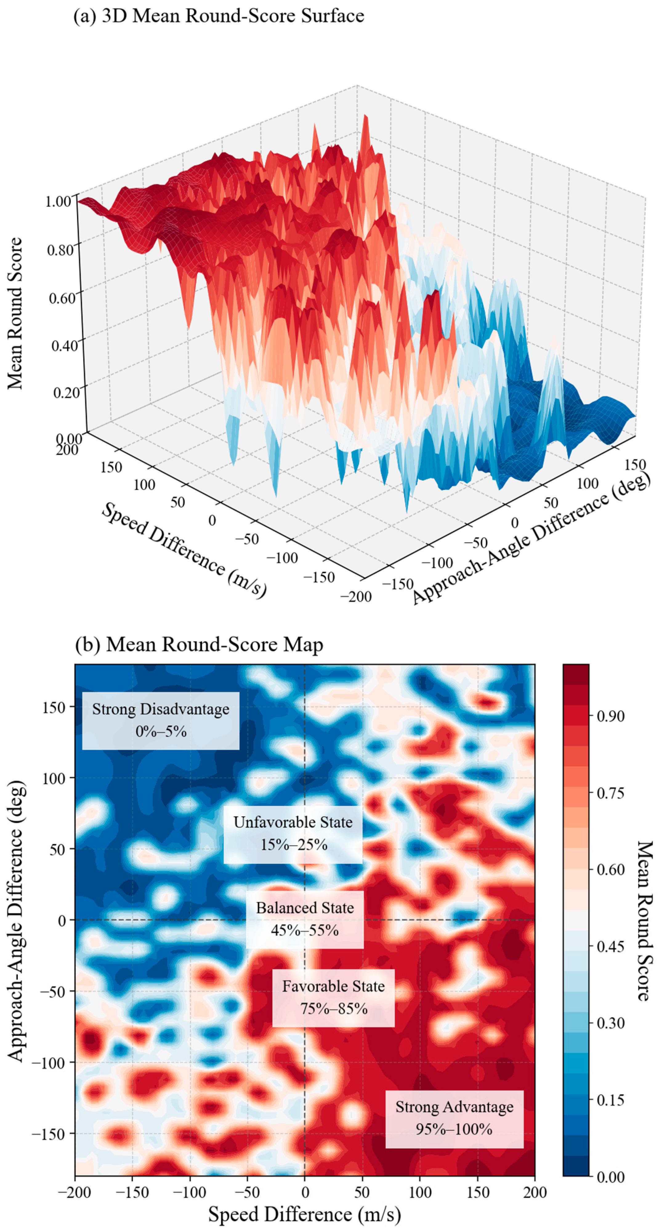
For speed–angle conversion, agent A remains at 300 m/s, agent B spans the preset speed range, both headings span 0–360 deg, and altitude is 7000 m. Figure 8 shows the resulting surface.

Figure 8 shows that a favorable rear approach and moderate speed advantage reinforce one another, whereas speed alone cannot fully compensate for an unfavorable angle.

The speed–angle surrogate uses standardized relative speed, a bounded half-angle dominance feature, and sparse interaction terms.

$$A_{\theta }=-sin\left(\Delta {\theta }_{rad}/2\right)$$

(9)

$$I_{v\theta }^{(1)}=x_v^2{A}_{\theta },\hspace{1em}{I}_{v\theta }^{(2)}=x_v{A}_{\theta }^2,\hspace{1em}{x}_v={\displaystyle \frac{\Delta v}{150}}$$

(10)

For trajectory replay, each agent’s approach angle is computed from its yaw–pitch heading vector and the local line of sight. We define Δθ = α_A − α_B, so a negative value favors agent A, and use A_θ = −sin(Δθ_rad/2), which is bounded to [−1, 1] and changes sign under label exchange. The released speed–angle basis contains x_v²A_θ and x_vA_θ² as its explicit speed–angle interactions; it does not contain a standalone x_vA_θ term.

$$\hat{p}\left(\Delta v,\Delta \theta \right)=clip\left({\beta }_0+{\displaystyle \sum }_i{\beta }_i{\varphi }_i\left(\Delta v,\Delta \theta \right),0,1\right)$$

(11)

The predictor is clipped to [0, 1] after label antisymmetrization. This definition is used identically by the Python runtime, generated CSV lookup tables, and NetLogo bridge.

The released speed–angle surface retains the favorable and unfavorable angular sectors represented in the benchmark calibration.

3.2.3. Conversion of Altitude and Angular Advantages

For altitude–angle conversion, agent A’s altitude and both headings vary over the preset ranges, agent B remains at 7000 m, and both start at 260 m/s.

The altitude–angle sweep shows that altitude advantage and a rear approach reinforce one another, whereas low altitude and unfavorable angle yield low score.

The altitude–angle surrogate uses x_h = Δh/1150, A_θ = −sin(Δθ_rad/2), and the released sparse odd and interaction terms. It follows the same clipped surrogate formulation as Equation (11), with the input variables replaced by (Δh, Δθ).

The retained altitude–angle basis and coefficients are listed explicitly in UDSA_model_parameters.csv; no hidden normalization or learned runtime state is used.

The released altitude–angle surface retains both high-advantage and near-balanced regions represented in the benchmark calibration.

Table A2. Retained coefficients of the released pairwise surrogates.

Surrogate	Linear Terms	Higher-Order Terms	Interaction Terms
Speed–altitude	1: 0.500; xv: 0.161; xh: 0.250	xv3: −0.011; xh3: −0.012; xv5: 0.0012; xh5: 0.0015	xv2 xh: 0.009; xv xh2: 0.013
Speed–angle	1: 0.500; xv: 0.148; Aθ: 0.226	xv3: −0.008; Aθ3: 0.015; xv5: 0.0008	xv2 Aθ: 0.009; xv Aθ2: 0.012
Altitude–angle	1: 0.500; xh: 0.202; Aθ: 0.219	xh3: −0.013; Aθ3: 0.014; xh5: 0.0009	xh2 Aθ: 0.010; xh Aθ2: 0.014

consolidates the retained coefficients for all three pairwise surrogates. The largest linear term is altitude in the speed–altitude model (0.250), angular dominance in the speed–angle model (0.226), and angular dominance in the altitude–angle model (0.219); the interaction terms retain positive signs, while the principal cubic corrections are negative except for the angular cubic terms.

4. Unified-Dimensional Situation Assessment Method

4.1. Advantage Conversion

Two heterogeneous advantages are equivalent when the calibrated surrogates predict the same mean round score under identical controlled variables. For k ∈ {v, θ}, the altitude equivalent h_k^* minimizes |f_k(x_k, 0) − f_h(0, h)| over h ∈ [−3000, 3000] m. Speed, angle, and their joint speed–angle state are converted separately, allowing the interaction contribution to remain explicit. For the joint speed–angle state, the same criterion is applied to f_vθ(Δv, Δθ), yielding h_vθ^* over the same bounded altitude interval.

$$h_k^{*}=\underset{h\in [-3000,3000]}{\arg \min }\left|f_k(x_k,0)-f_h(0,h)\right|,\hspace{1em}k\in \{v,\theta \}$$

(12)

The neutral score is 0.5 under mirrored labels. A 121-point scan locates exact sign-change brackets and the lowest-residual grid neighborhood before bounded golden-section refinement, avoiding a global monotonicity assumption. The altitude-equivalent search uses [−3000, 3000] m and stops when the local interval is no wider than 1 m or after 25 iterations. The 10⁻³ score tolerance defines the neutral shortcut. Multiple roots use the smallest sign-consistent magnitude. If no sign-change bracket exists, the implementation refines the best in-domain neighborhood and returns its minimum-residual candidate. A result is flagged as out_of_domain when the residual exceeds 0.02.

Algorithm 1 formalizes the safeguarded conversion used for each single-factor or joint source score. It combines a coarse scan, bounded local refinement, sign-consistent root selection, and the stated out-of-domain rule.

Algorithm 1. Safeguarded altitude-equivalent conversion.
Input	Source score p; altitude reference fh(0, h); h ∈ [−3000, 3000] m; 121 scan points; score tolerance 10−3; interval tolerance 1 m; residual limit 0.02; maximum 25 local iterations.
1	Evaluate p from the clipped source advantage.
2	If |p − 0.5| ≤ 10−3, return h* = 0 with neutral status.
3	Evaluate |fh(0, h) − p| on the 121-point altitude grid; retain exact roots, sign-change brackets, and the lowest-residual neighborhood.
4	Refine every retained bracket or neighborhood by bounded golden-section search until its width is ≤1 m or 25 iterations have elapsed.
5	From admissible roots, select the smallest |h*| whose sign agrees with p − 0.5; if no root exists, select the minimum-residual in-domain candidate.
6	Set out_of_domain when the final score residual exceeds 0.02.
Output	Altitude equivalent h*, score residual, iteration count, and domain-status flag.

Offline tables use 5 m/s and 2 deg grids and are linearly or bilinearly interpolated online. Across the released 5 m/s and 2 deg grids, 26,874 of 29,483 conversions invoked local refinement, and every refined case converged in nine iterations; 99 neutral cases used the 10⁻³ shortcut, and 2510 saturated cases coincided with exact grid roots. The mean score residual was 1.87 × 10⁻⁵ ± 3.65 × 10⁻⁵ (maximum 9.9952 × 10⁻⁴), and all conversions remained within the 0.02 domain criterion. On the same platform used in Section 6.4, a refined offline conversion took a median of 0.490 ms and 0.892 ms at the 95th percentile (0.588 ± 0.621 ms, mean ± sample standard deviation). The search generates offline equivalence tables; online evaluation uses table interpolation, with its timing reported in Section 6.4.

4.2. Unified-Dimensional Situation Assessment Based on a Unified Altitude-Equivalent Advantage Scale

Algorithm 2 assembles the unified altitude-equivalent state while retaining every component and diagnostic flag, as specified below.

Algorithm 2. UDSA on the unified altitude-equivalent scale.
Input	Signed differences Δv, Δh, and Δθ; calibrated domains; pairwise surrogates and lookup tables.
1	Clip each input to its calibrated domain and retain the input-domain flag.
2	Apply Algorithm 1 to the speed-only and angle-only source scores to obtain hv and hθ.
3	Apply Algorithm 1 to the joint speed–angle score to obtain hvθ.
4	Compute hint = hvθ − hv − hθ.
5	Assemble htotal = clip(Δh) + hv + hθ + hint.
6	Map htotal to S = 0.5[1 + tanh(clip(htotal, −3000, 3000)/1200)].
Output	S; hv, hθ, hvθ, hint, and htotal; residuals and combined domain-status flag.

The implementation uses S = 0.5[1 + tanh(clip(h_total, −3000, 3000)/1200)]. Thus S = 0.5 at h_total = 0, the scale is 1200 m, and all outputs remain in [0, 1]. These constants and all search tolerances are stored in config/udsa_config.json.

$$\begin{array}{l}{h}_c=\mathrm{clip}(h_{\mathrm{total}},-3000,3000)\\ S(h_{\mathrm{total}})=0.5[1+\tanh ({\displaystyle \frac{h_c}{1200}})]\end{array}$$

(13)

5. Situation Assessment-Based Balanced Expert Decision-Making for Robotic Games

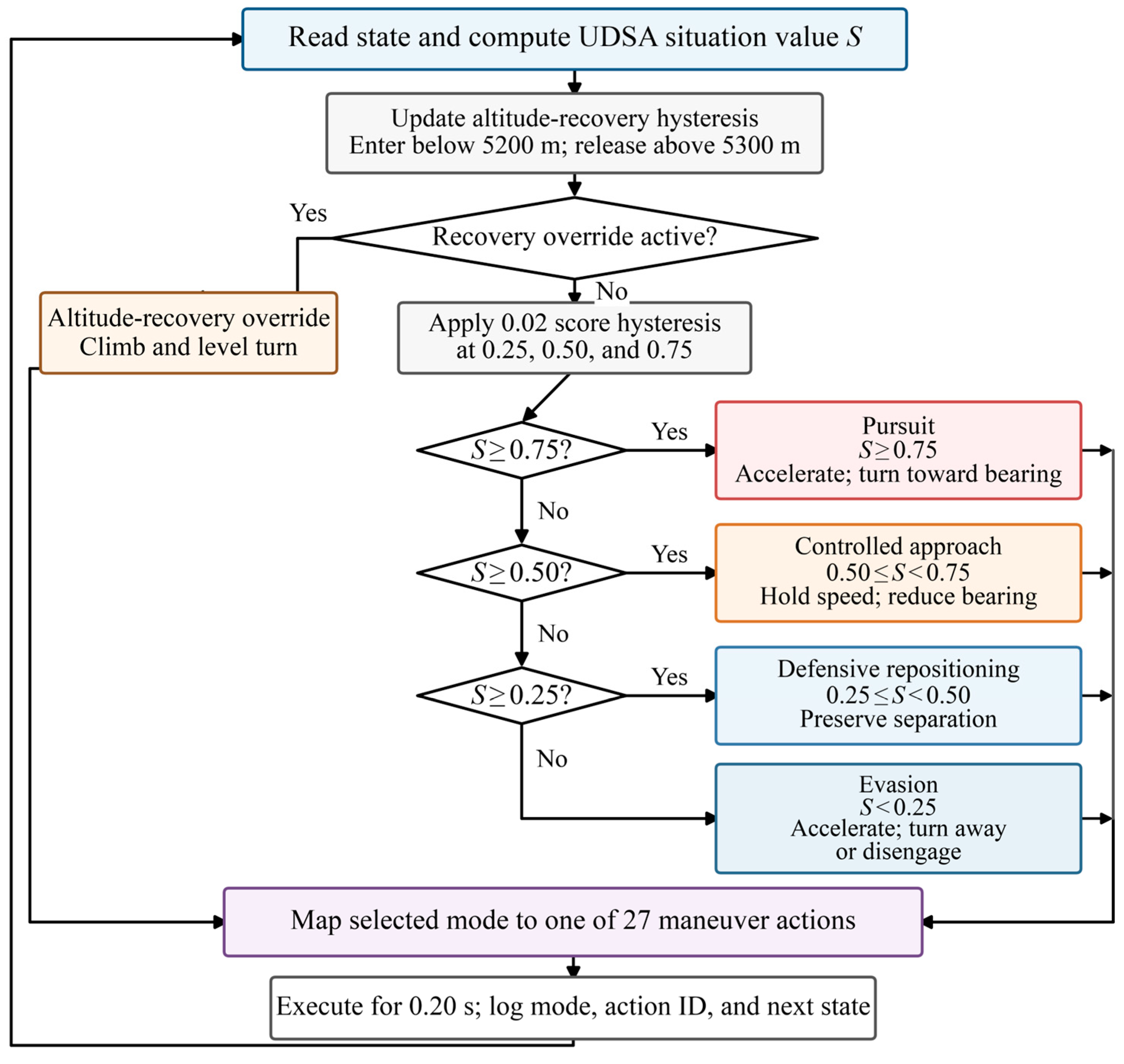
Figure 9 summarizes the SABED carrier used in the original closed-loop experiments. Altitude recovery overrides other modes below 5200 m and releases above 5300 m. Otherwise, S ≥ 0.75 selects pursuit, 0.50 ≤ S < 0.75 approach, 0.25 ≤ S < 0.50 repositioning, and S < 0.25 evasion; a 0.02 hysteresis band prevents chattering. Each mode maps to one of 27 maneuver actions.

6. Experiments and Results

6.1. Experimental Protocol and Statistical Analysis

The original comparison protocol held motion dynamics, frozen PER-DDQN weights, outcome rules, SABED thresholds, and scenario samples fixed while changing only the SA module. Every reported 500-round cell comprises five 100-round seed groups (1123, 2147, 3251, 4363, and 5479). The primary metric is mean round score, with wins, draws, and losses assigned 1, 0.5, and 0, respectively. The released round-level CSV supports raw wins/draws/losses, seed mean ± sample standard deviation, draw rate, and a 95% bootstrap percentile confidence interval from 10,000 within-seed resamples with analysis seed 20260728.

The original pairwise mixed-condition suite used 500 rounds per opponent and allocated head-on, crossing, and pursuit initial states in approximately equal proportions within each seed. Expert weighting used angular, altitude, and speed weights of 0.4, 0.25, and 0.35. CRITIC used a 10-sample trailing window and the classical information value σ_j Σ_k(1 − |r_jk|), normalized to unit sum. round_level_results.csv provides outcomes and seed assignments.

6.2. Pairwise Mixed-Condition Comparisons

Agent A uses UDSA and agent B uses expert-weighted SA; both use SABED, so only the SA module differs.

Table 3. Initial settings of closed-loop interaction experiment with expert experience-based situation assessment.

Agent	x-Coordinate (m)	y-Coordinate (m)	z-Coordinate (m)	Pitch Angle γ (rad)	Heading Angle φ (rad)	Speed (m/s)
Agent A	500–1500	3500–4500	7000–10,000	[$-\pi ∕4,\pi ∕4$]	[$0,2\pi$]	200–350
Agent B	500–1500	0–1000	7000–10,000	[$-\pi ∕4,\pi ∕4]$	[$0,2\pi$]	200–350

gives the initial settings.

Against expert weighting, the five-seed score was 0.790 ± 0.010, with 375/40/85 wins/draws/losses, an 8.0% draw rate, and a reproducible stratified-bootstrap 95% interval of 0.756–0.823.

UDSA is also compared with CRITIC-based SA, which derives weights from correlations among dominance factors. The conditions in Table 3 and the SABED policy are retained, and only agent B’s SA method changes.

Against CRITIC, the five-seed score was 0.710 ± 0.016, with 330/50/120 wins/draws/losses, a 10.0% draw rate, and a reproducible stratified-bootstrap 95% interval of 0.672–0.746.

The CRITIC draw rate was 2 percentage points above the expert-weighting comparison. In the released 427-snapshot UDSA-CRITIC trajectory subset, 73.3% of CRITIC values lay between 0.45 and 0.55 and their mean absolute distance from 0.5 was 0.033; the corresponding UDSA values were 30.0% and 0.094. This stronger concentration around the balanced region activates the midrange SABED modes more frequently, favoring conservative approach and repositioning sequences and thereby increasing the probability of unresolved rounds. Each draw contributes 0.5 to the reported metric, so the mean round score of 0.710 already incorporates this draw behavior.

6.3. Training Diagnostics, Baselines, and Extreme Conditions

Across five PER-DDQN seeds, convergence occurred at 3654 ± 160 episodes, final return was 7.84 ± 0.23, validation score was 0.762 ± 0.019, and the frozen policy scored 0.748 ± 0.021 on the held-out test set; all ± values are sample standard deviations calculated from PER_DDQN_training_summary.csv.

Table 4. Scenario-stratified method performance with raw outcome counts.

Method	Scenario Mean Scores (Head-On/Crossing/Pursuit)	Pooled W/D/L (n = 1500)	Pooled Score (Bootstrap 95% CI)
UDSA	0.840/0.795/0.810	1172/101/227	0.815 (0.796–0.833)
Expert Weighting	0.610/0.540/0.566	783/150/567	0.572 (0.548–0.595)
DRL-SA	0.780/0.742/0.752	1062/150/288	0.758 (0.738–0.778)
CRITIC	0.660/0.612/0.630	876/150/474	0.634 (0.611–0.657)
Entropy-TOPSIS	0.630/0.580/0.602	831/150/519	0.604 (0.580–0.627)

separates the head-on, crossing, and pursuit cells. In the original study, the deep reinforcement learning-based situation assessment (DRL-SA) comparator was a three-layer 128-64-1 multilayer perceptron trained on the same factor-sweep labels and frozen before closed-loop testing. PER-DDQN maps the five online state components to one of 27 maneuver actions and serves as the common maneuver policy, whereas DRL-SA maps dominance-factor inputs to a scalar SA value and replaces only the assessment module in its comparison cells. Entropy-TOPSIS estimated entropy weights from the normalized factor matrix and used closeness to the positive and negative ideal solutions. The released package contains their round-level outcomes.

Table 4 reports 7500 scenario-stratified rounds (five methods × three scenarios × five seeds × 100 rounds). Head-on, crossing, and pursuit use 5, 4, and 3 km of separation, respectively; all outcomes are retained without outlier filtering.

UDSA scored 0.815 (1172/101/227), versus 0.758 for DRL-SA, 0.634 for CRITIC, 0.604 for Entropy-TOPSIS, and 0.572 for expert weighting. All methods used the same frozen PER-DDQN carrier and paired scenario cells, so spatial variation in maneuver-policy competence was shared across the comparisons. UDSA exceeded DRL-SA by 0.060, 0.053, and 0.058 in the head-on, crossing, and pursuit strata, respectively, showing that the ranking persisted across the three sampled regions of the state space.

Table 5. Closed-loop stress tests with large initial speed and altitude differences.

Initial Condition for Agent A	vs Expert: Score (W/D/L)	vs CRITIC: Score (W/D/L)	vs Entropy-TOPSIS: Score (W/D/L)
Δv = −150 m/s, Δh = 0 m, Δθ = 90 deg	0.620 (285/50/165)	0.590 (270/50/180)	0.600 (275/50/175)
Δv = 0 m/s, Δh = −1500 m, Δθ = 90 deg	0.580 (265/50/185)	0.560 (255/50/195)	0.570 (260/50/190)
Δv = −150 m/s, Δh = −1500 m, Δθ = 90 deg	0.510 (230/50/220)	0.490 (220/50/230)	0.500 (225/50/225)
Δv = 150 m/s, Δh = 1500 m, Δθ = −90 deg	0.910 (440/30/30)	0.880 (425/30/45)	0.890 (430/30/40)

reports the four large-disparity stress conditions.

Each Table 5 cell contains five seeds × 100 rounds; UDSA remains above 0.5 under isolated disadvantage, reaches parity under combined disadvantage, and reaches at least 0.88 under combined advantage.

6.4. Empirical Symmetry, Sensitivity, and Runtime

Empirical self-play uses identical frozen UDSA-SABED modules, mirrored states, and exchanged labels for half of each seed. Across 1500 rounds, head-on (235/30/235), crossing (232/36/232), and pursuit (238/24/238) each score 0.500; their reproducible bootstrap intervals are 0.458–0.542, 0.459–0.543, and 0.457–0.542.

A deterministic one-factor-at-a-time sensitivity analysis was performed on the 2213 released trajectory snapshots. The tagging divisor in Equation (3), the 30 deg angular threshold, the 1200 m score-mapping scale, and the three SABED score thresholds were varied around their registered values while all trajectory states and fitted coefficients were held fixed.

Table 6. Sensitivity of tagging and SABED classifications on 2213 released trajectory snapshots.

Parameter	Tested Settings	Diagnostic at Tested Settings	Agreement with Baseline
Speed denominator in vi2/(C g)	C = 8/10/12	Valid-tag gate: 5.65%/5.42%/5.20%	99.77%/100%/99.77%
Angular threshold θth	25/30/35 deg	Valid-tag gate: 4.88%/5.42%/6.37%	99.46%/100%/99.05%
Score-mapping scale	960/1200/1440 m	Mean S: 0.381/0.384/0.389	Tier: 94.98%/100%/95.30%
SABED score thresholds	(0.20, 0.50, 0.80)/(0.25, 0.50, 0.75)/(0.30, 0.50, 0.70)	Mean S fixed at 0.384	Tier: 93.00%/100%/94.31%

reports the resulting gate rates, mean scores, and agreement of the discrete tag or SABED classification with the baseline configuration.

The 8 g and 12 g denominator variants changed only 5 of 2213 tag classifications relative to 10 g. A +/−20% change in the 1200 m mapping scale retained 94.98–95.30% of SABED tiers, and symmetric widening or narrowing of the outer score thresholds retained 93.00–94.31%. These perturbations change boundary occupancy as expected while preserving the dominant trajectory-level classifications. The complete deterministic output is provided in data/processed/parameter_sensitivity_summary.csv.

A 10,000-query replay benchmark of the released lookup implementation on macOS arm64 with Python 3.12 measured a median of 29.8 microseconds and 35.6 microseconds at the 95th percentile, approximately 0.015% of the 0.20 s decision interval.

7. Discussion and Limitations

UDSA improves the reported closed-loop score against the tested SA modules within the stated protocol. The common frozen PER-DDQN carrier, paired scenario cells, and consistent UDSA-DRL-SA margins across head-on, crossing, and pursuit conditions separate the assessment comparison from scenario-specific policy retraining. The sensitivity results further show stable discrete classifications around the registered tagging, mapping, and SABED parameters. Interpretability is provided by traceable features, equivalent conversion, explicit coefficients, and boundaries; the released sparse polynomial is a fixed empirical reference surrogate calibrated for this benchmark.

The original NetLogo environment enabled controlled sweeps but omitted rigid-body aerodynamics, actuators, stall, structural accumulation, sensing, communication, and weather. The −8 command, 10 g normalization, and 3000/1200 m constants are benchmark parameters; deployment requires higher-fidelity, hardware-in-the-loop, and flight validation.

Statistics treat 0/0.5/1 as a bounded score and report seed dispersion, W/D/L, and stratified bootstrap intervals. All seeds still share one simulator; self-play tests label invariance. Equilibrium analysis lies outside the present scope, and fitted surfaces require recalibration outside the stated envelope.

Future work will reproduce the benchmark in a second simulator, validate it in software/hardware-in-the-loop and flight tests, and extend it to teams, obstacles, uncertainty, energy limits, and safety filters.

8. Conclusions

This paper develops a traceable flying robotic game benchmark for closed-loop SA comparison. Reported controlled experiments characterize speed, altitude, and approach-angle advantages; safeguarded UDSA conversion handles multiple or absent equivalent solutions; and SABED provides the common decision carrier. PER-DDQN serves as the fixed maneuver carrier. The methodological contribution centers on UDSA factor conversion and controlled SA comparison. The released package reproduces the UDSA runtime, equivalence conversion, trajectory assessment, and reported statistical summaries. UDSA scored 0.790 ± 0.010 against expert weighting and 0.710 ± 0.016 against CRITIC, and led the scenario-stratified baselines at 0.815. Symmetric self-play returned 0.500, while stress tests bounded performance outside nominal conditions.

References

- Chung, T.H.; Hollinger, G.A.; Isler, V. Search and pursuit-evasion in mobile robotics. Auton. Robots 2011, 31, 299–316. [Google Scholar] [CrossRef] [Scilit]
- Brockman, G.; Cheung, V.; Pettersson, L.; Schneider, J.; Schulman, J.; Tang, J.; Zaremba, W. OpenAI Gym. arXiv 2016, arXiv:1606.01540. [Google Scholar] [CrossRef] [Scilit]
- Terry, J.K.; Black, B.; Grammel, N.; Jayakumar, M.; Hari, A.; Sullivan, R.; Santos, L.S.; Dieffendahl, C.; Horsch, C.; Perez-Vicente, R.; et al. PettingZoo: Gym for multi-agent reinforcement learning. Adv. Neural Inf. Process. Syst. 2021, 34, 15032–15043. [Google Scholar]
- Shah, S.; Dey, D.; Lovett, C.; Kapoor, A. AirSim: High-fidelity visual and physical simulation for autonomous vehicles. In Field and Service Robotics; Springer: Cham, Switzerland, 2018; pp. 621–635. [Google Scholar] [CrossRef] [Scilit]
- Panerati, J.; Zheng, H.; Zhou, S.; Xu, J.; Prorok, A.; Schoellig, A.P. Learning to fly: A gym environment with PyBullet physics for reinforcement learning of multi-agent quadcopter control. In Proceedings of the 2021 IEEE/RSJ International Conference on Intelligent Robots and Systems (IROS); IEEE: Piscataway, NJ, USA, 2021; pp. 7512–7519. [Google Scholar] [CrossRef] [Scilit]
- Hanover, D.; Loquercio, A.; Bauersfeld, L.; Romero, A.; Penicka, R.; Song, Y.; Cioffi, G.; Kaufmann, E.; Scaramuzza, D. Autonomous drone racing: A survey. IEEE Trans. Robot. 2024, 40, 3044–3067. [Google Scholar] [CrossRef] [Scilit]
- Kaufmann, E.; Bauersfeld, L.; Loquercio, A.; Muller, M.; Koltun, V.; Scaramuzza, D. Champion-level drone racing using deep reinforcement learning. Nature 2023, 620, 982–987. [Google Scholar] [CrossRef] [Scilit]
- Endsley, M.R. Toward a theory of situation awareness in dynamic systems. Hum. Factors 1995, 37, 32–64. [Google Scholar] [CrossRef] [Scilit]
- Yang, A.; Li, Z.; Li, B.; Xi, Z.; Gao, C. Air Combat Situation Assessment Based on Dynamic Variable Weight. Acta Armamentarii 2021, 42, 1553–1563. [Google Scholar] [CrossRef]
- Xi, Z.; Kou, Y.; Li, Y.; Li, Z.; Lv, Y. A Dynamic Air Combat Situation Assessment Model Based on Situation Knowledge Extraction and Weight Optimization. Aerospace 2023, 10, 994. [Google Scholar] [CrossRef] [Scilit]
- Fang, W.; Zhang, T.; Tan, K.; Tang, M. Air Combat Situation Assessment Based on Differential Window Generative Adversarial Network. Syst. Eng. Electron. 2024, 46, 2738–2746. [Google Scholar] [CrossRef]
- Diakoulaki, D.; Mavrotas, G.; Papayannakis, L. Determining objective weights in multiple criteria problems: The CRITIC method. Comput. Oper. Res. 1995, 22, 763–770. [Google Scholar] [CrossRef] [Scilit]
- Zhang, T.; Mo, H. Reinforcement Learning for Robot Research: A Comprehensive Review and Open Issues. Int. J. Adv. Robot. Syst. 2021, 18, 1–22. [Google Scholar] [CrossRef] [Scilit]
- Wong, A.; Bäck, T.; Kononova, A.V.; Plaat, A. Deep Multiagent Reinforcement Learning: Challenges and Directions. Artif. Intell. Rev. 2023, 56, 5023–5056. [Google Scholar] [CrossRef] [Scilit]
- Lowe, R.; Wu, Y.; Tamar, A.; Harb, J.; Abbeel, P.; Mordatch, I. Multi-agent actor-critic for mixed cooperative-competitive environments. Adv. Neural Inf. Process. Syst. 2017, 30, 6379–6390. [Google Scholar]
- Mnih, V.; Kavukcuoglu, K.; Silver, D.; Rusu, A.A.; Veness, J.; Bellemare, M.G.; Graves, A.; Riedmiller, M.; Fidjeland, A.K.; Ostrovski, G.; et al. Human-level control through deep reinforcement learning. Nature 2015, 518, 529–533. [Google Scholar] [CrossRef] [Scilit]
- Van Hasselt, H.; Guez, A.; Silver, D. Deep Reinforcement Learning with Double Q-Learning. Proc. AAAI Conf. Artif. Intell. 2016, 30, 2094–2100. [Google Scholar] [CrossRef] [Scilit]
- Schaul, T.; Quan, J.; Antonoglou, I.; Silver, D. Prioritized experience replay. arXiv 2016, arXiv:1511.05952. [Google Scholar] [CrossRef] [Scilit]
- Hessel, M.; Modayil, J.; Van Hasselt, H.; Schaul, T.; Ostrovski, G.; Dabney, W.; Horgan, D.; Piot, B.; Azar, M.; Silver, D. Rainbow: Combining Improvements in Deep Reinforcement Learning. Proc. AAAI Conf. Artif. Intell. 2018, 32, 3215–3222. [Google Scholar] [CrossRef] [Scilit]
- Kapturowski, S.; Ostrovski, G.; Dabney, W.; Quan, J.; Munos, R. Recurrent Experience Replay in Distributed Reinforcement Learning. In Proceedings of the International Conference on Learning Representations, New Orleans, LA, USA, 6–9 May 2019. [Google Scholar]
- Li, B.; Zhang, H.; He, P.; Wang, G.; Yue, K.; Neretin, E. Hierarchical Maneuver Decision Method Based on PG-Option for UAV Pursuit-Evasion Game. Drones 2023, 7, 449. [Google Scholar] [CrossRef] [Scilit]
- Yan, T.; Liu, C.; Gao, M.; Jiang, Z.; Li, T. A Deep Reinforcement Learning-Based Intelligent Maneuvering Strategy for the High-Speed UAV Pursuit-Evasion Game. Drones 2024, 8, 309. [Google Scholar] [CrossRef] [Scilit]
- Chen, J.; Yu, C.; Li, G.; Tang, W.; Ji, S.; Yang, X.; Xu, B.; Yang, H.; Wang, Y. Online Planning for Multi-UAV Pursuit-Evasion in Unknown Environments Using Deep Reinforcement Learning. IEEE Robot. Autom. Lett. 2025, 10, 8196–8203. [Google Scholar] [CrossRef] [Scilit]
- Wang, X.; Wang, M.; Bai, X.; Ma, Z.; Sun, K.; Li, J. EO-MADDPG: An Improved Reinforcement Learning Approach for Multi-UAV Pursuit-Evasion Games. Aerospace 2026, 13, 296. [Google Scholar] [CrossRef] [Scilit]
- Xu, Z.; Shao, S.; Han, Z. A DRL Framework for Autonomous Pursuit-Evasion: From Multi-Spacecraft to Multi-Drone Scenarios. Drones 2025, 9, 636. [Google Scholar] [CrossRef] [Scilit]
- Wilensky, U. NetLogo; Center for Connected Learning and Computer-Based Modeling, Northwestern University: Evanston, IL, USA, 1999; Available online: http://ccl.northwestern.edu/netlogo/ (accessed on 24 June 2026).
- Beard, R.W.; McLain, T.W. Small Unmanned Aircraft: Theory and Practice; Princeton University Press: Princeton, NJ, USA, 2012. [Google Scholar] [CrossRef] [Scilit]