Routed Prototype Adapters for Federated Financial Return Prediction with Frozen LLMs

Abstract

Financial return prediction increasingly relies on both financial text and structured market covariates, but adapting large language models across financial institutions remains difficult because raw data cannot be centralized and clients often exhibit heterogeneous, non-stationary market signals. This paper studies data-local federated financial return prediction with a frozen LLM, aiming to share useful cross-client adaptation while preserving client-specific predictive behavior. We propose a federated routed-adapter framework in which the server maintains a pool of lightweight adapter prototypes, each client selects a personalized mixture of these prototypes through projected directional routing, and local residual adapters are learned on private client data around the selected mixture. The server then maps uploaded residual updates back to the shared prototype space through an exact least-norm decomposition for communication-efficient aggregation. The framework keeps raw financial data and client-private prediction heads local, while uploaded residuals remain model updates and should not be interpreted as a formal privacy guarantee without additional mechanisms such as secure aggregation or differential privacy. Across FNSPID, Qlib CSI300/CSI800, and Open FinLLM forecasting benchmarks, our method achieves the best overall performance, improving CSI300 RankIC from $0.082$ to $0.087$ over the strongest federated PEFT baseline and reducing FNSPID MAE from $0.00537$ to $0.00482$. These results suggest that compositional shared adaptation with local residual personalization is a practical direction for financial LLM deployment under data-local, communication-constrained, and heterogeneous federated settings.

1. Introduction

Financial return prediction is a central problem in quantitative investment, risk management, and market intelligence, where even small improvements in predictive quality can translate into substantial economic value [1,2]. Recent progress in large language models (LLMs) has created new opportunities for exploiting unstructured financial text, such as news, filings, and analyst reports, together with structured market covariates [3]. Financial-report question-answering studies likewise demonstrate that retrieval augmentation and neural reranking can improve the extraction of decision-relevant evidence from long filings [4]. Related context-aware prediction studies in autonomous driving also suggest that LLMs can help convert heterogeneous scene contexts into downstream decision signals [5]. However, financial prediction remains challenging because market signals are noisy, non-stationary, and highly heterogeneous across institutions, sectors, data vendors, and trading horizons. Empirical evidence from cross-market volatility analysis further shows that risk relationships can vary materially across market regimes [6].

Existing research has made important progress along two directions. On the financial modeling side, structured forecasting models have advanced from recurrent and graph-based architectures to market-aware transformers that capture temporal and cross-stock dependencies [7,8,9,10], while recent financial LLMs and benchmarks have strengthened text understanding and financial reasoning capabilities [11,12,13,14,15]. LLM-based extraction of segment disclosures further shows that dispersed narrative and tabular report content can be converted into more complete and comparable structured financial information [16]. Yet, these methods are typically developed under centralized or single-model assumptions, where all data can be pooled and one adapted model is expected to serve all distributions. This assumption is often misaligned with real financial institutions, which cannot freely share private data and may face distinct local regimes, client flows, and target distributions. On the federated learning side, methods such as FedAvg, FedProx, SCAFFOLD, FedPer, FedRep, and Ditto have studied decentralized optimization and personalization under non-IID data [17,18,19,20,21,22]. More recently, federated PEFT and LoRA-based methods have reduced the cost of adapting foundation models in decentralized environments [23,24,25,26,27,28]. Nevertheless, the existing literature does not fully resolve the adaptation structure required by federated financial LLMs. Standard FL methods usually aggregate one global update, which can blur institution-specific market structures under non-IID clients. Personalized FL methods separate global and local components, but this separation is often fixed: a client either follows a single shared representation or keeps a private correction around it. Recent federated PEFT methods further reduce adaptation cost, but many of them focus on exact LoRA aggregation, heterogeneous ranks, selective sharing, or a dual global–local adapter split. These mechanisms are valuable, yet they still do not explicitly model the possibility that different financial clients may share several partially overlapping adaptation directions. This is a natural requirement in finance, where clients may differ by sector exposure, trading horizon, local news coverage, or market regime, while still sharing some common predictive signals.

This paper asks: How can a frozen LLM be adapted for federated financial return prediction when clients exhibit heterogeneous and time-varying financial signals? Our high-level idea is to replace the “one shared adapter fits all” paradigm with a small shared prototype space that can be composed differently by different clients. Each client uses a local calibration gradient to identify the shared prototype directions that are most compatible with its current predictive signal, forms a simplex mixture of these prototypes, and then learns a lightweight residual correction on private data. The server updates the prototype pool from client residuals without accessing raw financial records. This design preserves the scalability of parameter-efficient LLM adaptation, supports data-local federated training, and provides a structured mechanism for heterogeneous financial personalization.

Our contributions are summarized as follows:

• We formulate federated financial LLM adaptation as a compositional personalization problem. Instead of assuming a single global adapter or a fixed global–local split, we argue that financial clients should be able to share multiple adaptation directions and combine them according to local market signals.
• We propose a federated routed-adapter framework that integrates projected directional routing, simplex mirror-descent route updates, local residual learning, and least-norm residual-to-prototype decomposition. The individual mathematical tools are standard, but their integration provides a route-consistent adapter aggregation mechanism for frozen LLMs under heterogeneous financial clients.
• We provide extensive empirical evaluation across text-driven return prediction, structured stock-ranking benchmarks, and stock-movement classification tasks. Additional analyses examine routing stability, route entropy, partition robustness, communication and wall-clock cost, statistical significance, and the sensitivity to client participation and calibration batch size.

2. Related Work

2.1. Financial Forecasting with Structured and Textual Signals

Early neural financial forecasting systems mainly model historical prices, technical indicators, and cross-stock relations, and recent data-fusion forecasting studies further show that combining heterogeneous financial signals can improve prediction under complex market dynamics [29]. Recent time-series architectures also revisit activation design itself, using piecewise polynomial activations within time–frequency modeling to improve forecasting efficiency and accuracy [30]. Related work in dynamic engineering systems further demonstrate that machine-vision features can be coupled with physics-informed multiscale time–frequency operators for robust nonlinear state estimation [31]. Hybrid forecasting research in adjacent operational domains likewise shows that stacked combinations of tree-based learners and deep sequence models can exploit complementary predictive structure in demand forecasting [32]. Representative works exploit social text and price histories for stock movement prediction [7], concept-aware shared information among correlated stocks [8], multiple temporal trading patterns through routing adaptors [9], and market-guided cross-stock transformers [10]. Sparse-bottleneck forecasting provides a complementary approach to cross-variable modeling by retaining critical dependency paths while suppressing noisy and redundant interactions [33]. A closely related stock-trend framework combines hierarchical trading-day graphs with chaotic spatio-temporal modeling to capture cross-stock structure and nonlinear temporal dynamics across multiple equity markets [34]. Meta-learning-based graph wavelet modeling in high-speed rail dynamics also provides adjacent evidence that localized graph-frequency representations can support adaptable nonlinear subsystem models [35]. Recent resources such as Qlib [36] and FNSPID [15] further standardize structured market prediction and large-scale news–price alignment. In adjacent financial-risk applications, variational gradient flow generative modeling has also been used to identify rare fraudulent transactions under severe class imbalance [37]. Meanwhile, financial language models, including FinBERT [11], FinGPT [12], PIXIU [13], and FinBen [14], have shown the value of domain-specific financial text understanding. Hybrid document-routed retrieval likewise exposes and addresses the robustness–precision trade-off between whole-document routing and chunk-level retrieval in financial RAG [38]. Language anchor methods in visual anomaly detection similarly show that textual semantic anchors can provide useful weak supervision for domain-specific recognition tasks [39]. In an adjacent multimodal segmentation setting, dual-perspective prompts have also been used to align textual and visual representations for fine-grained structured prediction [40]. Structured mid-level supervision for tool-using language models further suggests that intermediate structured signals can improve how LLMs connect inputs to task-specific actions [41]. However, most existing financial forecasting and FinLLM methods assume centralized training or a single adapted model, which is often unrealistic for financial institutions with private data, heterogeneous client flows, and regime-dependent signals. In contrast, our method keeps financial data local and learns client-specific routed adapters over a shared prototype pool, enabling text-aware return prediction under federated institutional heterogeneity.

2.2. Federated Learning and Personalization Under Heterogeneity

Federated learning was introduced to train models from decentralized data without sharing raw samples [17]. Subsequent methods improve optimization under non-IID client distributions by proximal regularization [18], control variates [19], or data harmonization for confusion-resistant federated learning [42]. A parallel-line study personalized federated learning, where clients share part of the model while retaining personalized components, such as personalization layers [20], shared representations [21], or regularized local models [22]. These methods establish the importance of separating global and local knowledge, but they are usually designed for conventional neural networks and do not explicitly exploit the geometry of adapter mixtures in frozen LLMs. Our approach follows the global–local separation principle, but implements it through a simplex route over shared adapter prototypes and an additive client residual, thereby providing a structured form of personalization for federated financial LLM adaptation.

2.3. Federated Parameter-Efficient Tuning of Foundation Models

Parameter-efficient tuning, especially adapters [43] and LoRA [44], makes LLM adaptation feasible without updating all backbone parameters. Recent federated LLM methods combine this idea with FL, including federated instruction tuning and benchmarking frameworks [23,45], privacy-oriented or communication-efficient LoRA variants [46], heterogeneous-rank aggregation methods such as FLoRA [24] and FlexLoRA [25], local tuning without the full model [47], forward-pass-based federated tuning [48], dual global–local adapter designs [26,49], selective LoRA aggregation [27], exact LoRA aggregation [28], and prototype-aligned federated soft-prompt personalization [50]. Efficient reasoning studies also reduce LLM computation through skill-aware decomposition and distilled pruning, which is complementary to parameter-efficient adaptation [51]. Knowledge distillation provides another complementary route: recent time-series foundation-model research uses horizon-aware objectives and temporal representation alignment to retain forecasting quality in substantially smaller student models [52]. These works address important challenges such as communication, rank heterogeneity, privacy, and aggregation correctness. Nevertheless, most of them learn either a single global adapter or a fixed global/local decomposition, and they do not explicitly match clients to multiple shared adaptation directions according to task-sensitive gradient signals. Our method complements this literature by introducing projected directional routing over a prototype pool, followed by local residual learning and exact least-norm residual decomposition, which is particularly suited to heterogeneous financial clients and non-stationary market regimes.

2.4. Relation to Personalized Federated PEFT and Routing-Based Adaptation

Several recent methods have studied personalization for federated foundation models. FedDPA introduces a dual-personalizing adapter architecture in which global and local adapters are dynamically combined at test time, mainly to handle personalization and test-time distribution shifts [49]. FDLoRA similarly uses dual LoRA modules, where one branch captures global knowledge and the other captures client-specific knowledge [26]. FedSA-LoRA analyzes the asymmetry between LoRA matrices and selectively shares the LoRA A matrices while keeping more client-specific components local [27]. FedEx-LoRA focuses on exact aggregation for LoRA updates and corrects the inexactness of conventional federated LoRA averaging [28]. These methods address important aspects of federated PEFT, including aggregation correctness, selective sharing, and global–local personalization.

Our method differs in the structure of the shared adaptation space. Rather than learning one global adapter plus one local adapter, or deciding which LoRA factors should be shared, the server maintains multiple shared adapter prototypes. Clients form convex mixtures of these prototypes and update their routes through projected directional matching between local calibration gradients and prototype-update signatures. This makes the client–server interaction closer to client-level compositional routing than to a fixed global–local split. The broader idea of composing reusable primitives is also consistent with recent continual vision–language adaptation studies that align primitive compositions or maintain compositional concept memories [53,54]. It is also loosely aligned with cognitive-neuroscience evidence that conceptual combination and social semantic accumulation rely on structured semantic representations [55,56]. Joint semantic, affordance, and attribute parsing further illustrates how decomposed semantic factors can support structured representation learning [57]. Routing-oriented robot manipulation work also uses routing as a training-free mechanism for selecting policies under varying task contexts [58]. Router-guided multi-teacher distillation similarly uses routing to personalize which teacher signals are synthesized for a given target setting [59]. The least-norm decomposition is not claimed as a new linear-algebra result; its role is to ensure that a residual learned around a routed prototype mixture is mapped back to prototype space in a way that exactly reconstructs the client-side residual under the same route. This route-consistent aggregation geometry is the main structural distinction from dual-adapter and selective-aggregation methods.

The proposed routing mechanism is also related to mixture-of-experts and adapter-routing models, but the setting and signal are different. Standard MoE gating is usually token- or instance-level and learned by back-propagating a gating network. In contrast, our route is client-level and updated online from a calibration gradient, without training an additional server-side gating network or requiring raw client data at the server. KL mirror descent provides a simple simplex-constrained update with inertia from the previous route, which is useful when calibration gradients are noisy in federated financial streams.

Table 1. Structural comparison with closely related federated PEFT and routing-based methods.

Method	Shared Adaptation	Client Personalization	Routing Signal	Server Update
FedDPA	One global adapter	Local adapter and test-time weighting	Instance-wise weighting	Global adapter
FDLoRA	One global LoRA branch	Personalized LoRA branch and fusion	Adaptive fusion	Global LoRA branch
FedSA-LoRA	Shared LoRA A factors	Local LoRA B factors	Selective factor sharing	Selected LoRA factors
FedEx-LoRA	Exact global LoRA update	Optional local state	None	Exact LoRA correction
MoE/adapter routing	Expert pool	Token- or instance-level expert choice	Learned gate logits	Expert parameters
Ours	Multiple adapter prototypes	Client route and local residual	Projected calibration-gradient alignment	Route-consistent prototype residuals

summarizes these structural differences against the closest federated PEFT and routing-based methods. We also add two broader LLM-system references recommended by the reviewers to situate the work among federated LLM systems and LLM-enabled decision support [60,61].

3. Method

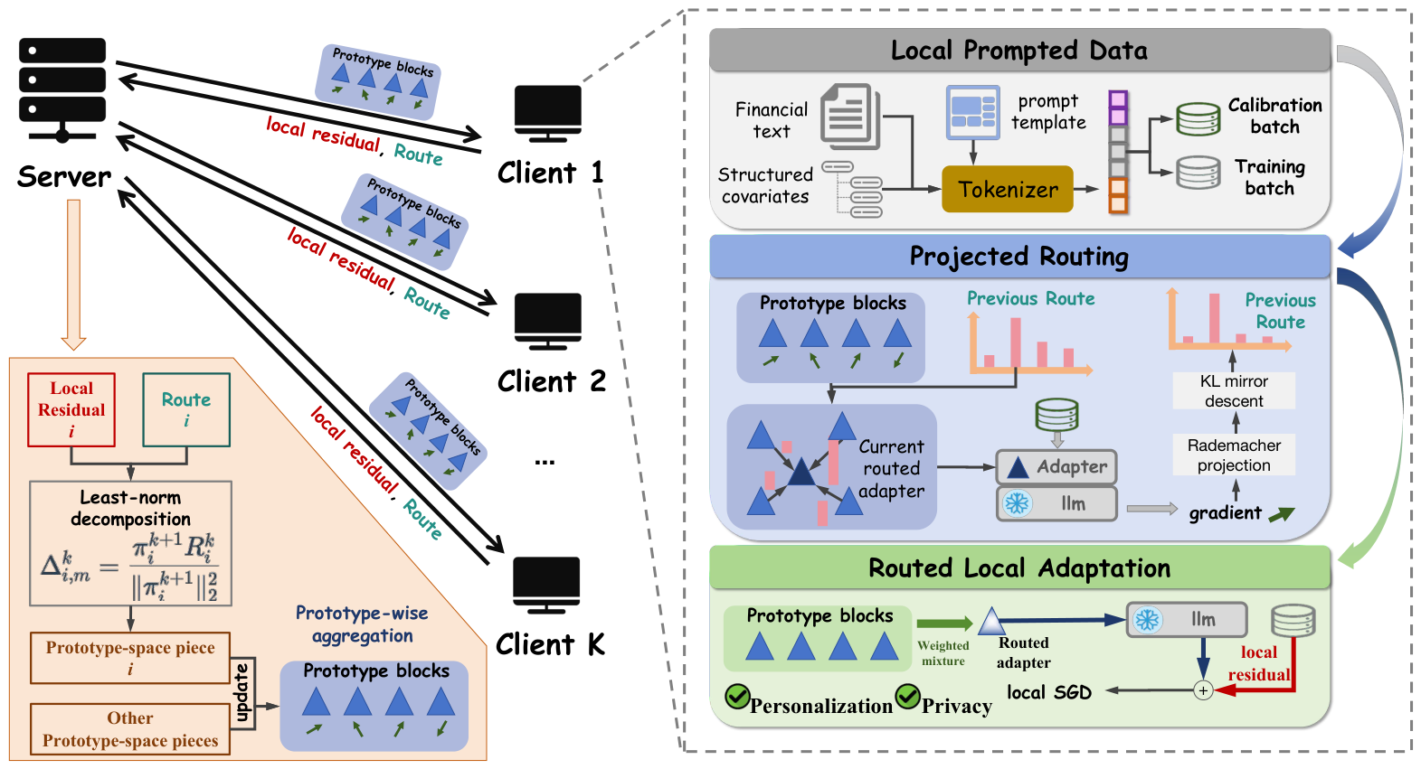
Figure 1 introduces the complete client–server workflow before the individual components are formalized. The server broadcasts a pool of shared adapter prototypes and their projected signatures. Each selected client constructs prompted financial inputs, computes a calibration gradient, updates a simplex route by projected directional matching and KL mirror descent, and learns an additive residual around the routed prototype mixture. The client keeps its raw data and prediction head local and uploads only its residual, updated route, and sample count. The server then maps each residual back to prototype space through the exact least-norm decomposition and aggregates the resulting prototype-wise updates. This separates shared adaptation, client personalization, and communication-efficient matching; further derivations are provided in Appendix A.

Appendix A 

Table A1. Main notation used in the routed-adapter method. 

Symbol	Meaning
K/M	Number of clients/number of shared adapter prototypes
k/${\mathcal{S}}_k$	Communication round/selected client set in round k
$A_m^k$	Prototype adapter object m maintained by the server
${\pi }_i^k$	Client i’s simplex route over prototype adapters
$R_i^k$	Local residual adapter learned by client i around its routed mixture
P/q	Public random projection matrix/projected routing dimension
${\mathbf{g}}_i^k$/${\tilde{\mathbf{g}}}_i^k$	Normalized calibration gradient/projected calibration gradient
$U_m^k$/${\mathbf{v}}_m^k$	EMA prototype-update accumulator/projected prototype signature
$s_{i,m}^k$	Directional alignment score between client i and prototype m
${\Delta }_{i,m}^k$/${\overline{\Delta }}_m^k$	Client-to-prototype decomposed residual/aggregated prototype residual

summarizes the notation used in the routing, residual-learning, and server-aggregation equations.

3.1. Prototype Pool and Personalized Prediction

A single globally shared adapter is too restrictive in federated finance because institutions can differ substantially in text source, market regime, client flow, and prediction target distribution. We therefore represent the shared adaptation space by a small pool of adapter prototypes and let each client assemble a personalized convex mixture from this pool. The mixture is low-dimensional, interpretable, and naturally compatible with communication-efficient federated training.

Client i owns a local time-indexed dataset ${\mathcal{D}}_i={\left\{({\mathbf{d}}_{i,t},{\mathbf{z}}_{i,t},y_{i,t+\tau })\right\}}_{t=1}^{T_i},$ where ${\mathbf{d}}_{i,t}$ is local financial text, ${\mathbf{z}}_{i,t}$ denotes structured covariates, and $y_{i,t+\tau }\in \mathbb{R}$ is the return over prediction horizon $\tau$. Each sample is converted into a textual prompt

$$x_{i,t}=\mathrm{Tok}\left(\mathcal{T}({\mathbf{d}}_{i,t},{\mathbf{z}}_{i,t})\right),{\tilde{\mathcal{D}}}_i={\left\{(x_{i,t},y_{i,t+\tau })\right\}}_{t=1}^{T_i},$$

(1)

where $\mathcal{T}(·)$ is the prompt template and $\mathrm{Tok}(·)$ is the tokenizer of the frozen LLM.

Let $f_{{\theta }_0}$ denote the pretrained LLM with frozen backbone parameters ${\theta }_0$. We insert trainable adapters into a set of layers $\mathcal{L}$. An adapter object is written as $A={\{\Delta W_{\ell }\}}_{\ell \in \mathcal{L}}.$ For adapter objects, addition and scalar multiplication are defined layer-wise,

$${\parallel A\parallel }_F^2=\sum _{\ell \in \mathcal{L}}{\parallel \Delta W_{\ell }\parallel }_F^2,$$

(2)

and $\mathrm{vec}(A)$ concatenates the vectorized updates of all adapted layers.

At round k, the server maintains a prototype pool ${\mathcal{P}}^k={\left\{A_m^k\right\}}_{m=1}^M.$ Each client i maintains a routing distribution

$${\mathit{\pi }}_i^k={({\pi }_{i,1}^k,\dots ,{\pi }_{i,M}^k)}^{\top }\in {\Delta }^{M-1},{\Delta }^{M-1}=\left\{\mathit{\pi }\in {\mathbb{R}}_{+}^M:{\displaystyle \sum _{m=1}^M}{\pi }_m=1\right\},$$

(3)

with initialization ${\mathit{\pi }}_i^0={\displaystyle \frac{1}{M}}\mathbf{1}$.

Given a routing distribution $\mathit{\pi }$, the corresponding mixed adapter is

$$A_i(\mathit{\pi };{\mathcal{P}}^k)={\displaystyle \sum _{m=1}^M}{\pi }_m{A}_m^k.$$

(4)

This mixed adapter serves as a client-specific point in the shared adaptation space.

For an input sequence x, the routed LLM representation is

$${\mathbf{h}}_i(x;\mathit{\pi },{\mathcal{P}}^k)=\mathrm{MeanPool}\left(f_{{\theta }_0,A_i(\mathit{\pi };{\mathcal{P}}^k)}(x)\right)\in {\mathbb{R}}^H,$$

(5)

and the local prediction head of client i is

$${\widehat{y}}_i(x;\mathit{\pi },{\mathcal{P}}^k)={\mathbf{w}}_i^{\top }{\mathbf{h}}_i(x;\mathit{\pi },{\mathcal{P}}^k)+b_i,$$

(6)

where $({\mathbf{w}}_i,b_i)$ are private client parameters and are never uploaded to the server. On a mini-batch $\mathcal{B}\subseteq {\tilde{\mathcal{D}}}_i$, the local regression loss is

$$F_i(A,{\mathbf{w}}_i,b_i;\mathcal{B})={\displaystyle \frac{1}{\left|\mathcal{B}\right|}}\sum _{(x,y)\in \mathcal{B}}{\displaystyle \frac{1}{2}}{\left({\mathbf{w}}_i^{\top }\mathrm{MeanPool}(f_{{\theta }_0,A}(x))+b_i-y\right)}^2.$$

(7)

The backbone ${\theta }_0$ remains frozen throughout training; only the routed adapter and the client-private head are updated.

3.2. Projected Directional Routing

The routing distribution should reflect which prototypes are currently most compatible with a client’s local task. A direct and task-sensitive signal is the local gradient direction with respect to the routed adapter. However, adapter gradients are high-dimensional. We therefore perform alignment in a low-dimensional projected space, which preserves directional geometry well while keeping routing inexpensive. This choice also follows the broader motivation of using invariant low-dimensional alignment signals in replay-free multimodal adaptation [62].

We fix a public Rademacher projection matrix

$$P\in {\left\{-{\displaystyle \frac{1}{\sqrt{q}}},+{\displaystyle \frac{1}{\sqrt{q}}}\right\}}^{q\times d},$$

(8)

where d is the number of adapter parameters and $q\ll d$ is the projection dimension. At round k, the server broadcasts projected prototype signatures ${\left\{{\mathbf{v}}_m^k\right\}}_{m=1}^M,{\mathbf{v}}_m^k\in {\mathbb{R}}^q,$ which summarize the recent update directions of the prototype pool; their server-side construction is given in Appendix A.2.

The prototype signature is constructed on the server from recent prototype update directions. Specifically, for each prototype m, the server maintains an exponential moving average accumulator $U_m^k$ with the same adapter-object shape as $A_m^k$. After receiving and aggregating decomposed residuals in round k, the server updates

$$U_m^{k+1}=(1-\lambda )U_m^k+\lambda {\overline{\Delta }}_m^k,$$

(9)

where $\lambda \in (0,1]$ is the signature momentum coefficient and ${\overline{\Delta }}_m^k$ is the aggregated prototype residual defined later in Equation (22). The projected prototype signature broadcast in the next round is

$${\mathbf{v}}_m^{k+1}={\displaystyle \frac{P\mathrm{vec}(U_m^{k+1})}{\parallel P\mathrm{vec}(U_m^{k+1}){\parallel }_2+\xi }}.$$

(10)

Thus, routing compares the client’s current calibration-gradient direction with a low-dimensional summary of each prototype’s recent update direction, rather than with the full prototype tensor itself.

Client i first forms its current routed adapter using the previous route,

$$A_i^k=A_i({\mathit{\pi }}_i^k;{\mathcal{P}}^k)={\displaystyle \sum _{m=1}^M}{\pi }_{i,m}^k{A}_m^k.$$

(11)

Using a calibration batch ${\mathcal{C}}_i^k\subseteq {\tilde{\mathcal{D}}}_i$, the client computes the normalized adapter gradient

$${\mathbf{g}}_i^k={\displaystyle \frac{\mathrm{vec}\left({\nabla }_A{F}_i(A_i^k,{\mathbf{w}}_i,b_i;{\mathcal{C}}_i^k)\right)}{{∥\mathrm{vec}\left({\nabla }_A{F}_i(A_i^k,{\mathbf{w}}_i,b_i;{\mathcal{C}}_i^k)\right)∥}_2+\xi }}\in {\mathbb{R}}^d,$$

(12)

where $\xi >0$ is a numerical constant, and projects it as ${\tilde{\mathbf{g}}}_i^k=P{\mathbf{g}}_i^k\in {\mathbb{R}}^q.$ The alignment score between client i and prototype m is then

$$s_{i,m}^k={\displaystyle \frac{\langle {\tilde{\mathbf{g}}}_i^k,{\mathbf{v}}_m^k\rangle }{\parallel {\tilde{\mathbf{g}}}_i^k{\parallel }_2{\parallel {\mathbf{v}}_m^k\parallel }_2+\xi }},m=1,\dots ,M.$$

(13)

Let ${\mathbf{s}}_i^k={(s_{i,1}^k,\dots ,s_{i,M}^k)}^{\top }$. We update the routing distribution by the KL mirror-descent step

$${\pi }_{i,m}^{k+1}={\displaystyle \frac{{\pi }_{i,m}^k\exp ({\eta }_{\pi }{s}_{i,m}^k)}{{\sum }_{j=1}^M{\pi }_{i,j}^k\exp ({\eta }_{\pi }{s}_{i,j}^k)}},m=1,\dots ,M,$$

(14)

where ${\eta }_{\pi }>0$ is the routing step size. This update keeps the route inside the simplex, preserves positivity, and performs multiplicative reweighting toward prototypes that are better aligned with the current local gradient.

The KL mirror-descent update also helps avoid abrupt hard assignment caused by a single noisy calibration batch. Because every coordinate is updated multiplicatively from ${\pi }_{i,m}^k$, a prototype with nonzero route weight remains reachable unless its probability is driven close to zero over many rounds. The step size ${\eta }_{\pi }$ controls the sharpness of this update: small values produce slow route adaptation, while overly large values can amplify calibration noise and cause premature concentration. To monitor this behavior, we track the normalized route entropy

$$H_i^k=-{\displaystyle \frac{1}{\log M}}{\displaystyle \sum _{m=1}^M}{\pi }_{i,m}^k\log {\pi }_{i,m}^k,$$

(15)

the collapse indicator $\mathbf{1}[{\max }_m{\pi }_{i,m}^k>0.9]$, and the prototype load $L_m^k={\left|{\mathcal{S}}_k\right|}^{-1}{\sum }_{i\in {\mathcal{S}}_k}{\pi }_{i,m}^k$ across communication rounds. These diagnostics are reported in Section 4.4.

3.3. Local Residual Learning and Federated Prototype Update

Once the routing distribution selects a client-specific mixture, the client should adapt around this routed point rather than overwrite the entire shared pool. At the same time, the server update must remain exactly compatible with the simplex mixture geometry. This concern resembles large-scale geometric adjustment settings, where relaxation-based solvers are used to preserve structural consistency under coupled variables [63]. We therefore let each client learn an additive residual around its routed adapter and then map this residual back to the prototype space through an exact least-norm decomposition before server aggregation.

After the routing update, client i forms the routed adapter

$${\widehat{A}}_i^k=A_i({\mathit{\pi }}_i^{k+1};{\mathcal{P}}^k)={\displaystyle \sum _{m=1}^M}{\pi }_{i,m}^{k+1}{A}_m^k.$$

(16)

Starting from $R_i=0$, the exact local optimum associated with the routed adapter is defined by

$$(R_i^{k,★},{\mathbf{w}}_i^{k,★},b_i^{k,★})\in \underset{R_i,{\mathbf{w}}_i,b_i}{\mathrm{arg\; min}}{F}_i({\widehat{A}}_i^k+R_i,{\mathbf{w}}_i,b_i;{\mathcal{B}}_i),$$

(17)

where ${\mathcal{B}}_i$ denotes the sequence of local training mini-batches in round k. Because this subproblem is non-convex, the implementation does not assume that the exact optimizer in Equation (17) is reached. Instead, starting from $R_i^{k,(0)}=0$ and the current private head, the client performs E AdamW steps and uses the final iterates $(R_i^k,{\mathbf{w}}_i^k,b_i^k):=(R_i^{k,(E)},{\mathbf{w}}_i^{k,(E)},b_i^{k,(E)})$ as a finite-step approximation.

The client uploads only $(R_i^k,{\mathit{\pi }}_i^{k+1},n_i)$, where $n_i$ is the local sample count used for aggregation. Raw financial data, local gradients, and the private head $({\mathbf{w}}_i,b_i)$ always remain local.

To update the prototype pool, the server reconstructs a prototype-space residual for each prototype by solving

$$({\Delta }_{i,1}^k,\dots ,{\Delta }_{i,M}^k)=\arg \underset{{\Delta }_1,\dots ,{\Delta }_M}{\min }{\displaystyle \sum _{m=1}^M}{\parallel {\Delta }_m\parallel }_F^2\mathrm{s}.\mathrm{t}.{\displaystyle \sum _{m=1}^M}{\pi }_{i,m}^{k+1}{\Delta }_m=R_i^k.$$

(18)

Its unique closed-form solution is

$${\Delta }_{i,m}^k={\displaystyle \frac{{\pi }_{i,m}^{k+1}}{\parallel {\mathit{\pi }}_i^{k+1}{\parallel }_2^2}}{R}_i^k,m=1,\dots ,M,$$

(19)

which satisfies the exact reconstruction identity

$${\displaystyle \sum _{m=1}^M}{\pi }_{i,m}^{k+1}{\Delta }_{i,m}^k=R_i^k.$$

(20)

Thus, the residual learned around the routed adapter is mapped back to prototype space without inconsistency.

This decomposition has a simple interpretation. The residual $R_i^k$ is learned around the mixed adapter ${\sum }_m{\pi }_{i,m}^{k+1}{A}_m^k$, but the server needs to update the individual prototypes. Equation (19) assigns the residual back to the prototype pool with the minimum total squared prototype perturbation while preserving the exact client-side residual under the same route. The route also determines how strongly a client affects each prototype:

$$\parallel {\Delta }_{i,m}^k{\parallel }_F={\displaystyle \frac{{\pi }_{i,m}^{k+1}}{\parallel {\mathit{\pi }}_i^{k+1}{\parallel }_2^2}}{\parallel R_i^k\parallel }_F.$$

(21)

For a one-hot route, only the selected prototype receives the residual. For a uniform route, all prototypes receive the same residual direction, and the weighted reconstruction remains exact. More generally, because ${\mathit{\pi }}_i^{k+1}\in {\Delta }^{M-1}$, we have ${\pi }_{i,m}^{k+1}/{\parallel {\mathit{\pi }}_i^{k+1}\parallel }_2^2\le \sqrt{M}$, so the per-client amplification is bounded by the prototype count. In practice, we monitor prototype update norms and route entropy to verify that no prototype is systematically over-updated.

Let ${\mathcal{S}}_k$ be the participating client set at round k, and let $N_k={\sum }_{i\in {\mathcal{S}}_k}{n}_i.$ The server computes the prototype-wise aggregated residual

$${\overline{\Delta }}_m^k={\displaystyle \frac{1}{N_k}}\sum _{i\in {\mathcal{S}}_k}{n}_i{\Delta }_{i,m}^k,m=1,\dots ,M,$$

(22)

and updates the prototype pool by

$$A_m^{k+1}=A_m^k+\beta {\overline{\Delta }}_m^k,m=1,\dots ,M,$$

(23)

where $\beta >0$ is the server learning rate. The server then refreshes the projected prototype signatures from the aggregated residuals and broadcasts ${\left\{(A_m^{k+1},{\mathbf{v}}_m^{k+1})\right\}}_{m=1}^M$ for the next round. A training round therefore consists of four stages: broadcast, projected routing, local residual learning, and prototype aggregation.

3.4. Algorithm Description and Complexity

Algorithm 1 summarizes the proposed training procedure. In each round, the server broadcasts the adapter prototypes and their projected signatures. Each selected client computes a calibration gradient, performs projected prototype matching, and updates its route by KL mirror descent. The updated route defines a personalized prototype mixture, around which the client learns an additive local residual using private data. The server then decomposes uploaded residuals into prototype-space pieces and aggregates them to update the shared prototype pool.

Algorithm 1 Federated Projected Routing with Local Residual Adapters

Require:  Client datasets ${\left\{{\mathcal{D}}_i\right\}}_{i=1}^K$, frozen LLM $f_{{\theta }_0}$, prototype number M, rounds R, local steps E, step sizes ${\eta }_{\pi },\beta$, projection P. Ensure:  Prototype pool ${\mathcal{P}}^R={\left\{A_m^R\right\}}_{m=1}^M$ and client routes ${\left\{{\mathit{\pi }}_i^R\right\}}_{i=1}^K$.   1: Initialize prototypes ${\mathcal{P}}^0={\left\{A_m^0\right\}}_{m=1}^M$, routes ${\mathit{\pi }}_i^0={\displaystyle \frac{1}{M}}\mathbf{1}$, private heads $({\mathbf{w}}_i,b_i)$, and signatures ${\left\{{\mathbf{v}}_m^0\right\}}_{m=1}^M$.   2: for  $k=0,\dots ,R-1$  do   3:        Server samples clients ${\mathcal{S}}_k$ and broadcasts ${\{A_m^k,{\mathbf{v}}_m^k\}}_{m=1}^M$.   4:        for all $i\in {\mathcal{S}}_k$ in parallel do   5:         Form prompted data and current routed adapter $A_i^k={\sum }_{m=1}^M{\pi }_{i,m}^k{A}_m^k$.   6:         Compute calibration gradient ${\mathbf{g}}_i^k={\displaystyle \frac{\mathrm{vec}({\nabla }_A{F}_i(A_i^k;{\mathcal{C}}_i^k))}{\parallel \mathrm{vec}({\nabla }_A{F}_i(A_i^k;{\mathcal{C}}_i^k)){\parallel }_2+\xi }}$ and projection ${\tilde{\mathbf{g}}}_i^k=P{\mathbf{g}}_i^k$.   7:         Compute alignment scores $s_{i,m}^k={\displaystyle \frac{\langle {\tilde{\mathbf{g}}}_i^k,{\mathbf{v}}_m^k\rangle }{\parallel {\tilde{\mathbf{g}}}_i^k{\parallel }_2{\parallel {\mathbf{v}}_m^k\parallel }_2+\xi }}$ for all m.   8:         Update route ${\pi }_{i,m}^{k+1}={\displaystyle \frac{{\pi }_{i,m}^k\exp ({\eta }_{\pi }{s}_{i,m}^k)}{{\sum }_{j=1}^M{\pi }_{i,j}^k\exp ({\eta }_{\pi }{s}_{i,j}^k)}}$.   9:         Form ${\widehat{A}}_i^k={\sum }_{m=1}^M{\pi }_{i,m}^{k+1}{A}_m^k$ and learn residual $R_i^k$ by E local SGD steps on $F_i({\widehat{A}}_i^k+R_i)$. 10:         Upload $(R_i^k,{\mathit{\pi }}_i^{k+1},n_i)$ to the server. 11:        end for 12:        Server decomposes ${\Delta }_{i,m}^k={\displaystyle \frac{{\pi }_{i,m}^{k+1}}{\parallel {\mathit{\pi }}_i^{k+1}{\parallel }_2^2}}{R}_i^k$ for all $i\in {\mathcal{S}}_k$ and m. 13:        Server updates $A_m^{k+1}=A_m^k+\beta {\displaystyle \frac{1}{N_k}}{\sum }_{i\in {\mathcal{S}}_k}{n}_i{\Delta }_{i,m}^k$ and refreshes ${\mathbf{v}}_m^{k+1}$ for all m. 14: end for 15: return ${\mathcal{P}}^R$ and ${\left\{{\mathit{\pi }}_i^R\right\}}_{i=1}^K$.

For each client, the routing overhead is $O(qd+Mq)$, where d is the adapter dimension, q is the projection dimension, and M is the number of prototypes. Local computation is dominated by E adapter-SGD steps, denoted by $O(E{C}_{\mathrm{sgd}})$. The server-side aggregation costs $O(|{\mathcal{S}}_k|Md)$ per round, and the upload cost per client is $O(d+M)$ for the residual and route. Since $M,q\ll d$, projected routing adds limited overhead compared with local adapter optimization.

Optimization Interpretation

The algorithm can be viewed as an approximate alternating procedure for the following personalized federated objective, whose optimum models are denoted explicitly:

$$\left({\{A_m^{★}\}}_{m=1}^M,{\{{\mathit{\pi }}_i^{★},R_i^{★},{\mathbf{w}}_i^{★},b_i^{★}\}}_{i=1}^K\right)\in \underset{\begin{array}{c}{\left\{A_m\right\}}_{m=1}^M,{\{{\mathit{\pi }}_i,R_i,{\mathbf{w}}_i,b_i\}}_{i=1}^K\\ {\mathit{\pi }}_i\in {\Delta }^{M-1}\forall i\end{array}}{\mathrm{arg\; min}}{\displaystyle \sum _{i=1}^K}{p}_i{F}_i\left({\displaystyle \sum _{m=1}^M}{\mathit{\pi }}_{i,m}{A}_m+R_i,{\mathbf{w}}_i,b_i\right).$$

(24)

The route update approximately adjusts ${\mathit{\pi }}_i$ using a calibration-gradient alignment signal, local SGD optimizes $R_i$ and the private head on client data, and the least-norm decomposition maps the resulting residual back to prototype-space increments that exactly reconstruct the client residual under the current route. Because the resulting problem is non-convex and the routing signal is stochastic, we do not claim a formal global convergence theorem. This solver-oriented view is consistent with recent surveys of global solvers in 3D vision, which emphasize robustness and empirical diagnostics for difficult non-convex estimation problems [64]. Instead, we report empirical convergence, route entropy, and prototype-load diagnostics to assess stability.

4. Experimental Results and Analysis

4.1. Experimental Setup

• Datasets. We evaluate our method on three groups of financial prediction benchmarks. For text-driven return prediction, we use FNSPID, which aligns financial news with stock prices and supports joint modeling of textual signals and market covariates [15]. For structured market prediction, we use the Qlib CSI300 and CSI800 benchmarks with Alpha158 and Alpha360 features, following the common stock-ranking protocol used by recent forecasting models such as MASTER [10,36]. For stock-movement classification, we further include the Open FinLLM forecasting suite [7,65,66]. All datasets are split chronologically to avoid look-ahead bias. In the federated setting, we construct clients by sector-level stock groups when sector metadata is available; otherwise, we use Dirichlet non-IID partitions over stock identities with concentration parameter $\alpha =0.3$.
• Evaluation metrics. For return regression, we report MSE and MAE. For cross-sectional stock ranking, we report IC, RankIC, ICIR, RankICIR, annualized return (AR), information ratio (IR), annualized volatility (AV), and maximum drawdown (MDD), following Qlib-style evaluation protocols [10,36]. For stock-movement classification, we report Accuracy and Matthews correlation coefficient (MCC), consistent with Open FinLLM forecasting tasks [65]. For federated learning, we additionally report macro-averaged client performance, worst-quartile client performance, trainable parameters, and communication cost per round.
• Compared methods. We compare with four groups of baselines. First, we include standard and personalized FL methods: Local-only, FedAvg [17], FedAvgM [67], FedProx [18], SCAFFOLD [19], FedPer [20], FedRep [21], and Ditto [22]. Second, we compare with federated PEFT and LLM fine-tuning methods, including FedIT [23], FFA-LoRA [46], FLoRA [24], FlexLoRA [25], FedBiOT [47], FwdLLM [48], FedDPA [49], FDLoRA [26], FedSA-LoRA [27], and FedEx-LoRA [28]. Third, we include financial forecasting baselines commonly used in stock-ranking benchmarks, including XGBoost [68], LightGBM [69], CatBoost [70], LSTM [71], GRU [72], TCN [73], Transformer [74], GAT [75], ALSTM [76], HIST [8], and MASTER [10]. Finally, we compare with financial LLM baselines, including FinBERT [11], FinGPT [12], PIXIU [13], PloutosGPT [77], and StockLLM [78].
• Implementation details. We use Llama-3.2-1B-Instruct as the frozen backbone and insert LoRA-style adapters into the attention projection layers. The adapter rank is $r=8$, LoRA scaling is 16, and adapter dropout is $0.05$. We use $K=20$ clients for FNSPID and Qlib, $K=10$ clients for smaller movement-prediction datasets, and sample $25\%$ of clients per communication round. The default number of prototypes is $M=4$, the projection dimension is $q=256$, the routing step size is ${\eta }_{\pi }=0.1$, the server step size is $\beta =1.0$, and each selected client performs $E=3$ local SGD steps per round. The calibration batch size and local training batch size are both 16. We optimize adapter residuals and prediction heads with AdamW using learning rates $2\times {10}^{-4}$ and $1\times {10}^{-3}$, respectively. All experiments are repeated with three random seeds and run on four NVIDIA A100 80GB GPUs with bfloat16 training.

Fair Comparison Protocol

For all direct federated LLM/PEFT competitors, we use the same frozen Llama-3.2-1B-Instruct backbone, the same client partitions, the same chronological train/validation/test splits, the same maximum sequence length, the same number of communication rounds, the same client sampling ratio, and the same local-update budget. Adapter ranks or bottleneck dimensions are tuned on the validation split so that trainable parameters are within $10\%$ of our method unless a method requires a fixed structure by design. Financial LLM baselines such as FinGPT, PIXIU/FinMA, PloutosGPT, and StockLLM are reported as non-federated financial-LLM references unless explicitly equipped with the same federated PEFT protocol; they are not treated as direct federated competitors. Centralized structured forecasting models such as MASTER are non-private reference baselines trained on pooled market covariates. Communication costs include both server-to-client download and client-to-server upload payloads under bf16 transmission, excluding optimizer states because optimizer states are maintained locally or server-side and are not transmitted per round.

Table 2. Baseline configuration and fairness protocol.

Method	Setting	Backbone	Input	Adapter/Model Head	Trainable Params	Rounds	Local Steps	Client Sampling	LR
Local-only	Federated, no aggregation	Llama-3.2-1B	Same as ours	LoRA rank $r=8$ + private head	2.10 M	100/50	3	–	$2\times {10}^{-4}$/${10}^{-3}$
FedAvg	Federated	Llama-3.2-1B	Same as ours	LoRA rank $r=8$ + private head	2.10 M	100/50	3	25%	$2\times {10}^{-4}$/${10}^{-3}$
FedProx	Federated	Llama-3.2-1B	Same as ours	LoRA rank $r=8$ + private head	2.10 M	100/50	3	25%	$2\times {10}^{-4}$/${10}^{-3}$
SCAFFOLD	Federated	Llama-3.2-1B	Same as ours	LoRA rank $r=8$ + private head	2.10 M	100/50	3	25%	$2\times {10}^{-4}$/${10}^{-3}$
Ditto	Federated personalized	Llama-3.2-1B	Same as ours	Global LoRA + local model	4.20 M	100/50	3	25%	$2\times {10}^{-4}$/${10}^{-3}$
FLoRA	Federated PEFT	Llama-3.2-1B	Same as ours	LoRA, rank tuned within 10% params	2.05 M	100/50	3	25%	$2\times {10}^{-4}$/${10}^{-3}$
FedDPA	Federated PEFT	Llama-3.2-1B	Same as ours	Global/local adapters	2.24 M	100/50	3	25%	$2\times {10}^{-4}$/${10}^{-3}$
FedSA-LoRA	Federated PEFT	Llama-3.2-1B	Same as ours	Shared A, local B LoRA	2.08 M	100/50	3	25%	$2\times {10}^{-4}$/${10}^{-3}$
FedEx-LoRA	Federated PEFT	Llama-3.2-1B	Same as ours	Exact LoRA aggregation	2.12 M	100/50	3	25%	$2\times {10}^{-4}$/${10}^{-3}$
Ours	Federated PEFT	Llama-3.2-1B	Same as ours	$M=4$ prototypes + route + residual	2.31 M	100/50	3	25%	$2\times {10}^{-4}$/${10}^{-3}$
FinGPT/PIXIU/PloutosGPT/StockLLM	Non-federated reference	Original or matched backbone where applicable	Text or serialized features	Original method	1 B–7 B	–	–	–	–
MASTER/XGBoost/LightGBM	Centralized structured reference	Structured model	Market covariates	Original model	0.4 M–12 M	–	–	–	–

lists the matched backbone, input, adapter configuration, trainable parameters, communication rounds, local steps, client sampling ratio, and learning rates used for the comparison.

4.2. Main Results

• Overall comparison on stock-ranking benchmarks. 

  Table 3. Main results on Qlib CSI300 and CSI800 stock-ranking benchmarks.

  Category	Method	CSI300				CSI800
  		IC ↑	RankIC ↑	AR ↑	IR ↑	IC ↑	RankIC ↑	AR ↑	IR ↑
  Centralized forecasting	XGBoost	0.051	0.050	0.230	1.90	0.040	0.047	0.080	0.60
  	LSTM	0.049	0.051	0.200	2.00	0.028	0.039	0.090	0.90
  	GRU	0.052	0.052	0.190	1.50	0.039	0.044	0.070	0.60
  	TCN	0.050	0.049	0.180	1.40	0.038	0.045	0.050	0.40
  	Transformer	0.047	0.051	0.220	2.00	0.040	0.048	0.130	1.10
  	GAT	0.054	0.041	0.190	1.30	0.043	0.042	0.100	0.70
  	MASTER	0.064	0.076	0.270	2.40	0.052	0.066	0.280	2.30
  Personalized FL	Local-only	0.055	0.064	0.232	2.01	0.045	0.055	0.183	1.53
  	FedAvg	0.058	0.068	0.244	2.12	0.048	0.059	0.212	1.75
  	FedProx	0.059	0.069	0.250	2.18	0.049	0.060	0.221	1.84
  	SCAFFOLD	0.060	0.071	0.259	2.27	0.050	0.062	0.238	1.96
  	Ditto	0.062	0.073	0.270	2.38	0.052	0.065	0.264	2.16
  Federated PEFT	FLoRA	0.063	0.075	0.279	2.48	0.053	0.067	0.279	2.31
  	FlexLoRA	0.064	0.076	0.284	2.51	0.053	0.067	0.283	2.34
  	FedDPA	0.065	0.078	0.291	2.56	0.054	0.068	0.287	2.37
  	FedSA-LoRA	0.066	0.080	0.298	2.62	0.055	0.070	0.293	2.42
  	FedEx-LoRA	0.068	0.082	0.307	2.70	0.056	0.071	0.303	2.49
  Ours		0.072	0.087	0.331	2.91	0.059	0.075	0.333	2.73

  Note: Dark, medium, and light blue shading denote the best, second-best, and third-best results, respectively. ↑ indicate that higher values are better, respectively.

  reports the main comparison on the Qlib CSI300 and CSI800 benchmarks. We include centralized stock-forecasting models as non-private reference baselines and compare our method with representative personalized FL and federated PEFT methods under the same client partition and communication protocol. Our method achieves the best performance across all reported ranking and portfolio metrics. Compared with the strongest centralized reference, MASTER, our method improves IC/RankIC from $0.064/0.076$ to $0.072/0.087$ on CSI300 and from $0.052/0.066$ to $0.059/0.075$ on CSI800. Among federated baselines, FedEx-LoRA is generally the strongest competitor, but it still underperforms our method, suggesting that exact adapter aggregation alone is insufficient for heterogeneous financial clients. The consistent gains of our method indicate that projected routing and local residual learning provide effective client-specific adaptation while preserving a shared prototype space.
• Results on text-driven return prediction and stock-movement classification. 

  Table 4. Main results on text-driven return prediction and stock-movement classification. FNSPID reports MAE and MSE, where MSE is scaled by ${10}^{-4}$. BigData22, ACL18, and CIKM18 report accuracy and MCC.

  Method	FNSPID		BigData22		ACL18		CIKM18
  	MAE ↓	MSE ↓	Acc. ↑	MCC ↑	Acc. ↑	MCC ↑	Acc. ↑	MCC ↑
  LSTM	0.02493	17.00	51.00	0.010	53.00	0.060	53.00	0.020
  Transformer	0.00544	0.50	52.74	0.041	55.16	0.083	54.87	0.041
  DTML	0.01273	3.20	52.00	0.070	57.44	0.191	58.62	0.045
  StockNet	0.01346	3.80	53.00	0.000	58.23	0.081	56.37	0.023
  SLOT	0.01084	1.90	55.00	0.100	59.00	0.210	56.00	0.090
  FinGPT	0.00687	0.81	54.72	0.064	56.12	0.109	55.86	0.053
  PIXIU/FinMA	0.00672	0.78	51.00	0.020	56.28	0.104	53.24	−0.031
  PloutosGPT	0.00635	0.70	56.03	0.116	61.21	0.205	59.89	0.064
  StockLLM	0.00619	0.67	56.58	0.119	60.76	0.218	60.41	0.098
  FedAvg	0.00658	0.74	56.27	0.112	60.02	0.197	59.33	0.083
  FLoRA	0.00621	0.66	56.83	0.123	60.94	0.212	60.12	0.094
  FedDPA	0.00596	0.59	57.08	0.132	61.45	0.222	60.56	0.103
  FedSA-LoRA	0.00571	0.52	57.42	0.137	61.96	0.231	60.88	0.112
  FedEx-LoRA	0.00537	0.46	57.81	0.145	62.34	0.239	61.27	0.121
  Ours	0.00482	0.38	58.63	0.162	63.19	0.258	62.18	0.138

  Note: Dark, medium, and light blue shading denote the best, second-best, and third-best results, respectively. ↑ and ↓ indicate that higher and lower values are better, respectively.

  further evaluates whether the proposed routed-adapter framework can exploit textual financial signals. On FNSPID, our method obtains the lowest MAE and MSE, outperforming both conventional sequence models and financial LLM baselines. On the Open FinLLM forecasting datasets, our method consistently achieves the highest ACC and MCC on BigData22, ACL18, and CIKM18. The improvement is particularly clear on MCC, which is more informative under class imbalance. These results suggest that the proposed method does not merely improve average prediction accuracy, but also produces more balanced directional decisions. The advantage over PloutosGPT and StockLLM indicates that federated prototype routing can provide additional robustness beyond direct financial instruction tuning, especially when client distributions are heterogeneous.

Statistical Significance

Because improvements in financial RankIC can be numerically small but economically meaningful, we report statistical significance against the strongest federated baselines in

Table 5. Paired significance test on daily RankIC series.

Dataset	Comparison	Mean Difference	95% CI	p-Value	Significant at 0.05?
CSI300	Ours–FedEx-LoRA	0.005	[0.0021, 0.0078]	0.004	Yes
CSI300	Ours–FedSA-LoRA	0.007	[0.0039, 0.0102]	<$0.001$	Yes
CSI800	Ours–FedEx-LoRA	0.004	[0.0013, 0.0065]	0.012	Yes
FNSPID MAE	FedEx-LoRA–Ours	0.00055	[0.00021, 0.00088]	0.006	Yes

. For each seed, we compute daily RankIC series on the test period and compare methods using paired tests with block bootstrap confidence intervals over trading weeks. This evaluates whether the observed performance gap is stable over time rather than driven by a few test days.

As shown in Table 5, the improvements over FedEx-LoRA and FedSA-LoRA remain significant on the daily RankIC series, and the FNSPID MAE reduction is also significant under the paired test.

4.3. Ablation and Analysis

• Single-factor ablation. We conduct single-factor ablations to isolate the contribution of each key design component. All variants are evaluated under the same backbone, client partition, communication budget, and training protocol as the full model.

  Table 6. Single-factor ablation results on CSI300, FNSPID, and the Open FinLLM average.

  Variant	CSI300		FNSPID		Open FinLLM Avg.
  	IC ↑	RankIC ↑	MAE ↓	MSE ↓	Acc. ↑	MCC ↑
  Ours full model	0.0718	0.0871	0.00482	0.38	61.33	0.186
  w/o prototype pool ($M=1$)	0.0659 (−0.0059)	0.0792 (−0.0079)	0.00548 (+0.00066)	0.56 (+0.18)	59.74 (−1.59)	0.151 (−0.035)
  w/o projected routing, fixed uniform route	0.0676 (−0.0042)	0.0810 (−0.0061)	0.00524 (+0.00042)	0.49 (+0.11)	60.18 (−1.15)	0.159 (−0.027)
  w/o KL mirror descent	0.0689 (−0.0029)	0.0832 (−0.0039)	0.00508 (+0.00026)	0.45 (+0.07)	60.56 (−0.77)	0.168 (−0.018)
  full-dimensional routing without projection	0.0711 (−0.0007)	0.0862 (−0.0009)	0.00491 (+0.00009)	0.40 (+0.02)	61.04 (−0.29)	0.181 (−0.005)
  w/o local residual learning	0.0647 (−0.0071)	0.0778 (−0.0093)	0.00556 (+0.00074)	0.60 (+0.22)	59.42 (−1.91)	0.146 (−0.040)
  w/o least-norm decomposition	0.0668 (−0.0050)	0.0803 (−0.0068)	0.00536 (+0.00054)	0.54 (+0.16)	59.86 (−1.47)	0.154 (−0.032)
  w/o prototype-signature refresh	0.0679 (−0.0039)	0.0817 (−0.0054)	0.00529 (+0.00047)	0.51 (+0.13)	60.05 (−1.28)	0.157 (−0.029)

  Note: Dark shading denote the best results. ↑ and ↓ indicate that higher and lower values are better, respectively.

  reports representative results on CSI300, FNSPID, and the averaged Open FinLLM movement-classification benchmarks. The small blue numbers beside each result denote the performance degradation relative to the full model; for error metrics, positive values indicate increased error.

As shown in Table 6, removing local residual learning causes the largest degradation, reducing CSI300 RankIC by $0.0093$ and Open FinLLM average MCC by $0.040$. This confirms that learning a client-specific residual around the routed adapter is crucial for capturing institution-specific financial patterns. Removing the prototype pool also leads to a clear drop, with CSI300 IC decreasing from $0.0718$ to $0.0659$, showing that a single global adapter is insufficient under heterogeneous client distributions. The fixed-route variant performs worse than the full model across all benchmarks, which verifies the benefit of projected directional routing for client-prototype matching. The variant without KL mirror descent is also consistently weaker, suggesting that multiplicative simplex updates provide more stable route adaptation than one-shot score normalization. Finally, replacing the least-norm decomposition with a naive prototype update substantially hurts both ranking and classification metrics, indicating that preserving the mixture geometry during server aggregation is important for maintaining a coherent shared prototype space.

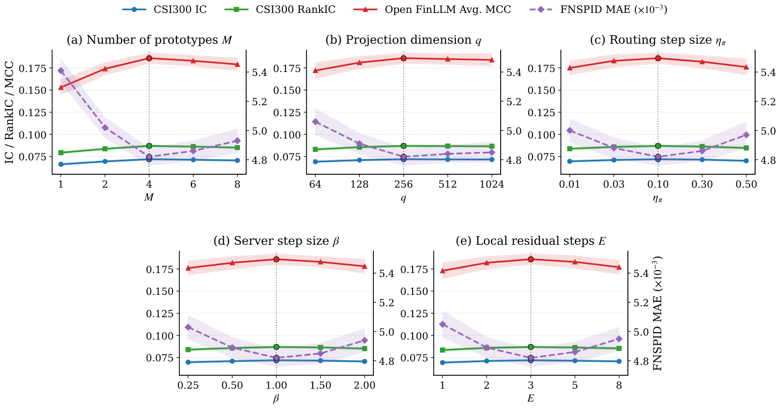
• Parameter sensitivity analysis. We further study the sensitivity of our method to key hyperparameters, including the number of prototypes M, projection dimension q, routing step size ${\eta }_{\pi }$, server update rate $\beta$, and local residual steps E. For each group, we vary one hyperparameter while keeping the others at the default configuration. Figure 2 reports mean and standard deviation over three random seeds. Overall, the performance remains stable across a broad range of values, showing that our method is not sensitive to a narrow hyperparameter choice.

As shown in Figure 2, the method is generally robust to moderate hyperparameter changes. For the number of prototypes, $M=1$ clearly underperforms because a single adapter cannot represent heterogeneous client regimes, while overly large M slightly degrades performance due to fragmented prototype usage and noisier routing. For the projection dimension, performance improves from $q=64$ to $q=256$ and then saturates, indicating that a moderate random projection is sufficient to preserve useful gradient-direction information. The routing step size ${\eta }_{\pi }$ also shows a stable middle range: too small a value slows route adaptation, whereas too large a value makes the route overreact to noisy calibration batches. The server update rate $\beta$ follows a similar pattern, where very small values update the prototype pool too conservatively and very large values amplify client-side residual noise. Finally, increasing local residual steps from $E=1$ to $E=3$ improves personalization, but further increasing E brings limited gains and can slightly hurt performance due to local drift. These trends are consistent with the design of our framework, which relies on a balance between shared prototype learning and client-specific residual adaptation.

4.4. Routing Stability and Calibration Sensitivity

To examine whether the route update suffers from premature prototype collapse, we track normalized route entropy, collapse rate, prototype load, and route-change magnitude across communication rounds. We also vary the calibration batch size $|{\mathcal{C}}_i^k|\in \{4,8,16,32,64\}$ while keeping other hyperparameters fixed. Smaller calibration batches produce noisier gradient directions and can increase route variance, whereas larger batches stabilize routing at the cost of additional local computation. In our default setting, $|{\mathcal{C}}_i^k|=16$ provides a stable trade-off between routing reliability and per-round cost.

Table 7. Calibration batch-size sensitivity. Collapse rate is the fraction of clients with ${\max }_m{\pi }_{i,m}>0.9$ averaged over the last 20 rounds.

Calibration Batch Size	CSI300 RankIC	Route Entropy ↑	Collapse Rate ↓	Time/Round (s)
4	0.0826	0.49	0.24	43.2
8	0.0849	0.57	0.16	45.1
16	0.0870	0.64	0.08	47.9
32	0.0871	0.67	0.05	52.8
64	0.0866	0.69	0.04	62.3

Note: ↑ and ↓ indicate that higher and lower values are better, respectively.

reports the batch-size trade-off, and

Table 8. Route dynamics over communication rounds with the default calibration batch size.

Round	Route Entropy ↑	Collapse Rate ↓	Load Imbalance ↓	Mean Route Change ↓
10	0.78	0.02	0.06	0.081
25	0.71	0.04	0.09	0.052
50	0.66	0.06	0.11	0.031
75	0.64	0.08	0.13	0.022
100	0.63	0.08	0.13	0.018

Note: ↑ and ↓ indicate that higher and lower values are better, respectively.

reports the route dynamics under the default setting.

As shown in Table 7, increasing the calibration batch from 4 to 16 improves RankIC and reduces collapse, while further increasing it yields limited accuracy gains but higher time per round. Table 8 shows that route entropy decreases smoothly rather than collapsing abruptly, indicating that clients become more specialized as prototypes learn distinct update directions. The low final collapse rate and the bounded load imbalance show that all prototypes remain active, while the decreasing route-change magnitude indicates that the route update stabilizes over training.

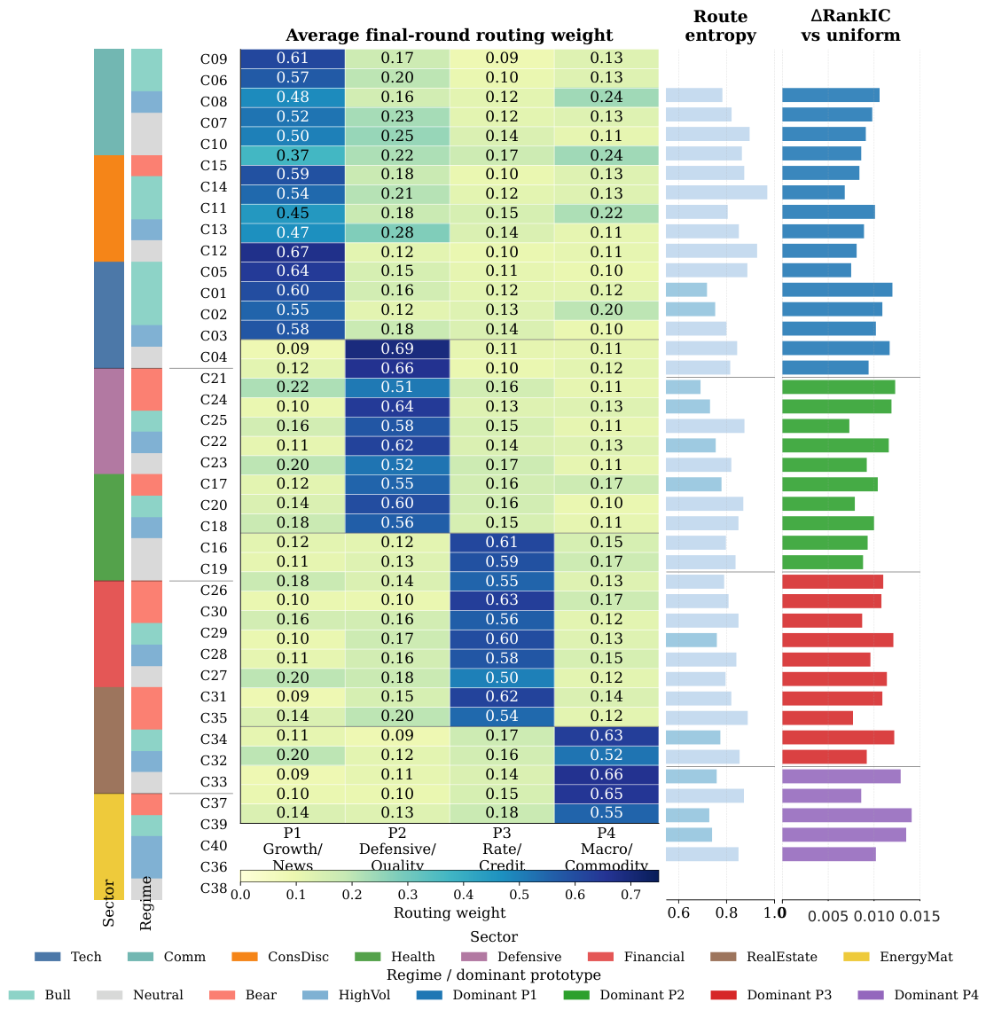
• Does routing capture client heterogeneity? To verify whether the learned routing distribution reflects client heterogeneity, we visualize the average final-round route of each client over the prototype pool. Specifically, for client i, we compute

  $${\overline{\mathit{\pi }}}_i={\displaystyle \frac{1}{\left|\mathcal{K}\right|}}\sum _{k\in \mathcal{K}}{\mathit{\pi }}_i^k,$$

  (25)

  where $\mathcal{K}$ denotes the last 20 communication rounds. We also report each client’s normalized route entropy and its RankIC improvement over the uniform-routing variant. The clients are sorted by their dominant prototype and sector annotation.

As shown in Figure 3, the learned routes exhibit a clear block structure. Technology, communication, and consumer-discretionary clients concentrate more on Prototype 1, defensive and healthcare clients mainly select Prototype 2, financial and real-estate clients are routed toward Prototype 3, while energy/materials clients under high-volatility or bear regimes rely more on Prototype 4. This suggests that the prototype pool learns functionally different adaptation directions rather than redundant copies of the same adapter. Moreover, clients with more concentrated routes usually obtain larger gains over uniform routing, especially in high-volatility or bear regimes. This supports the motivation of projected routing: client-specific prototype matching is most useful when local financial signals deviate from the global average pattern.

4.4.1. Partition Robustness Beyond Sector Grouping

The sector-based partition is useful for constructing realistic institutional heterogeneity, but it may also make some routing patterns visually align with the partition design. We therefore additionally evaluate routing behavior under random IID and Dirichlet partitions in

Table 9. Partition robustness of routing behavior on CSI300.

Partition	RankIC	Gain over Uniform Route	Route Entropy	Prototype Load Imbalance	Corr. Heterogeneity–Gain
Random IID	0.082	0.001	0.83	0.04	0.18
Dirichlet $\alpha =1.0$	0.084	0.003	0.75	0.08	0.36
Dirichlet $\alpha =0.3$	0.086	0.005	0.66	0.14	0.51
Dirichlet $\alpha =0.1$	0.088	0.007	0.57	0.21	0.63
Sector-based	0.087	0.006	0.62	0.18	0.58

. Under IID partitions, client routes are less concentrated and the gain over uniform routing is smaller. Under stronger Dirichlet heterogeneity, routes become more specialized and routing gains increase. This analysis tests whether routing captures measured client heterogeneity rather than merely recovering sector labels.

Table 9 confirms that routing gains grow as measured heterogeneity increases: the gain over uniform routing is only $0.001$ under random IID partitions but reaches $0.007$ under Dirichlet $\alpha =0.1$.

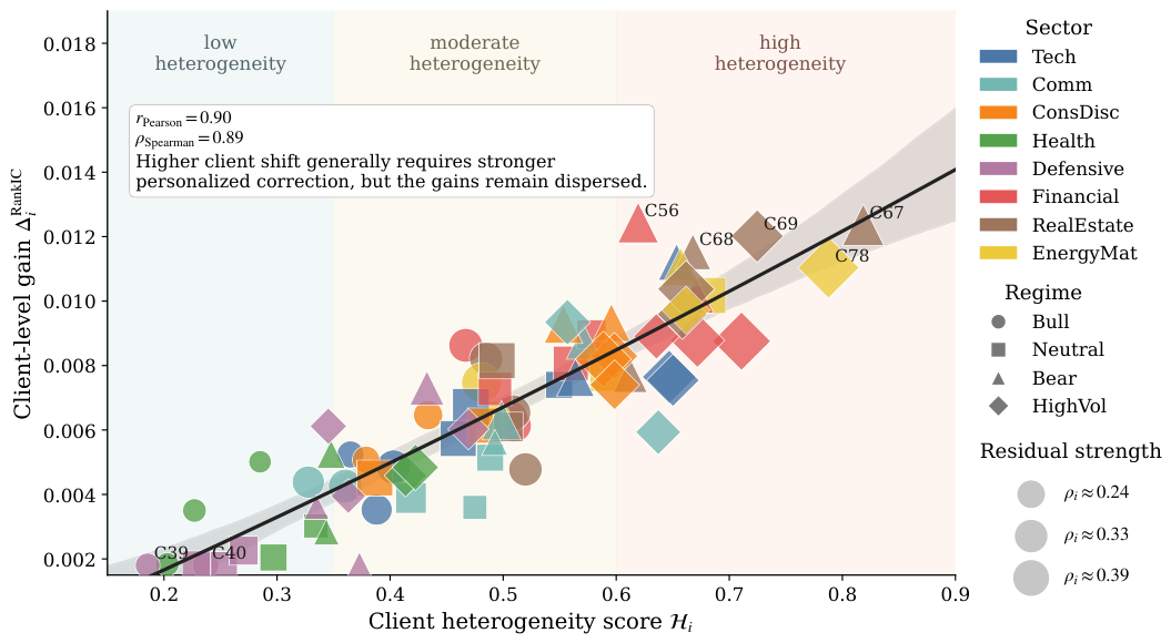
• Does the residual serve personalized adaptation? We further analyze whether the local residual mainly benefits clients with stronger distributional heterogeneity. For each client i, we compute a heterogeneity score

  $${\mathcal{H}}_i=\mathrm{JSD}(p_i(y)\parallel p_{\mathrm{global}}(y))+\lambda {\displaystyle \frac{\parallel {\mathsf{\mu }}_i^z-{\mathsf{\mu }}_{\mathrm{global}}^z{\parallel }_2}{\frac{1}{K}{\sum }_{j=1}^K{\parallel {\mathsf{\mu }}_j^z-{\mathsf{\mu }}_{\mathrm{global}}^z\parallel }_2}},$$

  (26)

  where $p_i(y)$ denotes the local return-label distribution and ${\mathsf{\mu }}_i^z$ denotes the mean structured-covariate vector of client i. We then compare the full model with the variant without local residual learning and measure the client-level gain

  $${\Delta }_i^{\mathrm{RankIC}}={\mathrm{RankIC}}_i^{\mathrm{Full}}-{\mathrm{RankIC}}_i^{\mathrm{w}/\mathrm{o}\mathrm{residual}}.$$

  (27)

  We also compute the normalized residual strength ${\rho }_i= \parallel R_i{\parallel }_F/{\parallel {\widehat{A}}_i\parallel }_F$ to quantify how much client-specific correction is learned around the routed adapter.

Figure 4 shows a clear positive relationship between client heterogeneity and the benefit of local residual learning. Low-heterogeneity clients cluster near the lower-left region, where the routed prototype mixture is already sufficient and only a small residual is needed. In contrast, high-volatility or bear-regime clients exhibit larger residual norms and larger RankIC gains, indicating that the residual captures local corrections that cannot be fully represented by the shared prototype pool. This supports the role of residual learning as a personalized adaptation mechanism rather than a uniform parameter expansion.

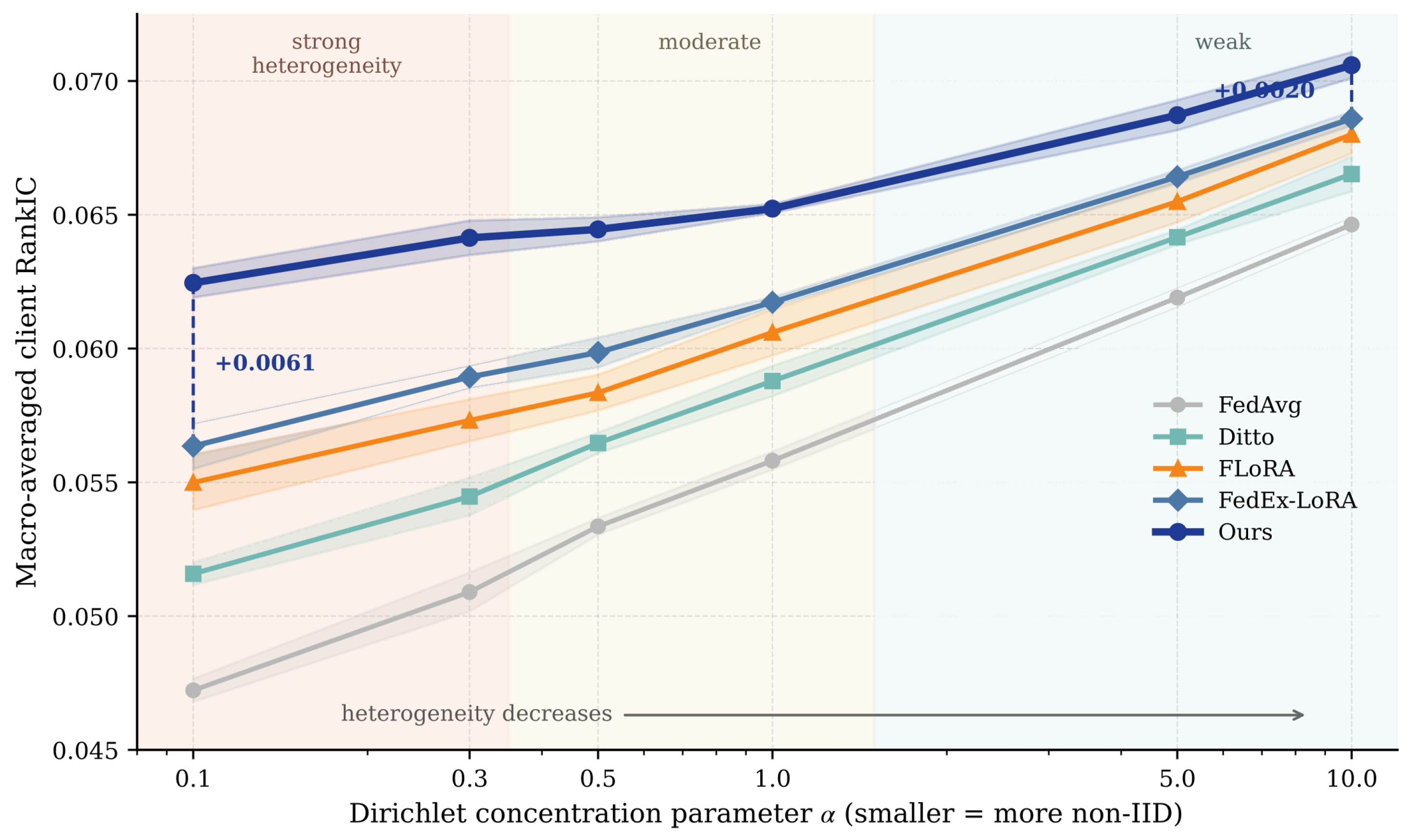
• Is our method more useful under stronger client heterogeneity? We further vary the degree of client heterogeneity using a Dirichlet partition over stock identities. Specifically, we sample client assignments with concentration parameter $\alpha \in \{0.1,0.3,0.5,1.0,5.0,10.0\}$, where smaller $\alpha$ indicates stronger non-IID heterogeneity. All methods are trained under the same backbone, communication rounds, and local-update budget. We report the macro-averaged client RankIC over three random seeds on the CSI300 benchmark.

As shown in Figure 5, all methods improve as $\alpha$ increases and the client distributions become less heterogeneous, but our method remains consistently superior across all settings. More importantly, the advantage of our method is largest in the strongly non-IID regime. For example, at $\alpha =0.1$, our method outperforms the strongest baseline, FedEx-LoRA, by about $0.0061$ in RankIC, whereas the margin decreases to about $0.0020$ at $\alpha =10.0$. This trend is consistent with the design of our method: projected routing helps identify more suitable shared prototypes when client distributions diverge, while local residual learning further compensates for client-specific deviations that cannot be absorbed by the shared prototype pool alone. Therefore, the benefit of our method becomes more pronounced exactly in the heterogeneous regime where federated financial modeling is most challenging.

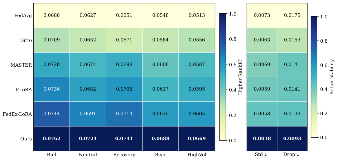
• Is the method more stable across market regimes? We further evaluate whether the proposed routed prototype adaptation remains robust under changing market conditions. We partition the CSI300 test period into five mutually exclusive market regimes using only the benchmark index close price. Let $r_t=\log (P_t/P_{t-1})$, $R_t^{(h)}={\sum }_{j=0}^{h-1}{r}_{t-j}$, and ${\sigma }_t^{(20)}=\sqrt{252}\mathrm{sd}(r_{t-19:t})$. The return cutoffs $c_{30}$ and $c_{70}$ are the 30th and 70th percentiles of $R_t^{(60)}$, and the volatility cutoff $v_{80}$ is the 80th percentile of ${\sigma }_t^{(20)}$, all estimated once on the 2008–2014 training split and then frozen. Test days are labeled in the following priority order: HighVol if ${\sigma }_t^{(20)}>v_{80}$; Bear if $R_t^{(60)}<c_{30}$ and $R_t^{(20)}\le 0$; Recovery if $R_t^{(60)}<c_{30}$ and $R_t^{(20)}>0$; Bull if $R_t^{(60)}>c_{70}$; and Neutral otherwise. This precedence makes every day belong to exactly one regime and prevents test-period information from entering the thresholds.

For each regime, we report the macro-averaged client RankIC on CSI300. To measure stability, we additionally summarize each method by the standard deviation across regimes and the worst-regime drop, defined as the gap between its best and worst-regime performances.

Figure 6 shows that all methods perform best in Bull and Recovery markets and deteriorate under Bear and HighVol regimes, which is consistent with the increased difficulty of financial prediction under market stress. However, our method maintains the highest RankIC in every regime and preserves a particularly clear advantage in the stressed regimes, where client distributions are more heterogeneous and less aligned with the global average. For example, under HighVol, our method reaches a RankIC of $0.0669$, compared with $0.0608$ for MASTER and $0.0605$ for FedEx-LoRA. Moreover, the right panel shows that our method has both the smallest cross-regime standard deviation and the smallest worst-regime drop, indicating that the gain is not limited to favorable market conditions. These results support the claim that prototype routing and local residual adaptation improve not only average performance, but also robustness to regime shift.

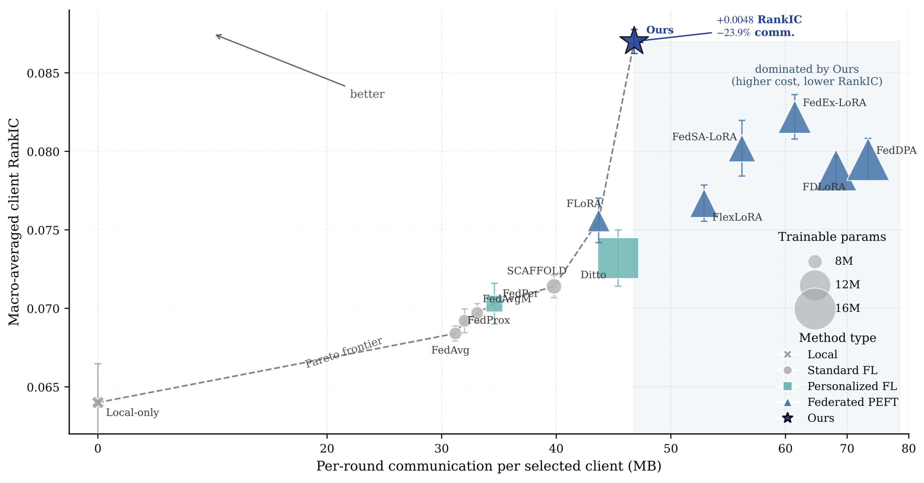
• Does the method achieve a better performance–communication trade-off? We finally analyze the trade-off between predictive performance and communication efficiency. For each federated method, we measure the per-round communication cost per selected client, including both download and upload payloads. The performance axis reports macro-averaged client RankIC on CSI300, the bubble size denotes the number of trainable parameters, and the vertical bars show the standard deviation over three seeds. A method is Pareto-efficient if no other method achieves higher RankIC with lower communication cost.

As shown in Figure 7, our method achieves the best RankIC while maintaining a moderate communication budget. Compared with FedEx-LoRA, our method improves RankIC from $0.0822$ to $0.0870$ while reducing per-round communication from $61.5$ MB to $46.8$ MB. Compared with FedSA-LoRA and FedDPA, it achieves larger gains with substantially lower communication cost. Low-cost methods such as FedAvg and FedProx are more communication-efficient, but their performance is much lower under heterogeneous clients. These results show that the proposed routed prototype design improves not only effectiveness but also the practical efficiency of federated financial adaptation.

For our method, the per-selected-client communication cost is computed as

$$\mathrm{Download}=M\left|A\right|b+Mqb,\mathrm{Upload}=\left|R\right|b+Mb+b_n,$$

(28)

where $\left|A\right|$ is the number of parameters in one prototype adapter, $\left|R\right|$ is the number of residual adapter parameters, q is the projection dimension, M is the number of prototypes, b is the number of bytes per transmitted scalar, and $b_n$ denotes the negligible sample-count payload. Unless otherwise stated, we use bf16 transmission and count both prototype downloads and residual uploads. We do not include optimizer states because they are not transmitted between the server and clients in our implementation. For baselines, we apply the same accounting rule to their transmitted adapter or LoRA payloads.

Table 10. Communication and wall-clock accounting.

Method	Download MB	Upload MB	Total MB/Round	Time/Round (s)	CSI300 RankIC
FedAvg	16.8	16.8	33.6	42.5	0.068
FedDPA	39.2	39.2	78.4	55.8	0.078
FedSA-LoRA	31.1	23.1	54.2	48.6	0.080
FedEx-LoRA	30.8	30.7	61.5	50.4	0.082
Ours	34.6	12.2	46.8	47.9	0.087

provides the resulting communication and wall-clock accounting for the main federated methods.

4.4.2. Sensitivity to Client Participation

We vary the client participation ratio in $\{10\%,25\%,50\%,100\%\}$ and report final RankIC, route entropy, convergence speed, and wall-clock cost in

Table 11. Client participation sensitivity on CSI300.

Participation Ratio	RankIC	Rounds to 95% Best Validation RankIC	Final Route Entropy	Time/Round (s)
10%	0.083	74	0.69	42.1
25%	0.087	58	0.64	47.9
50%	0.088	52	0.61	59.4
100%	0.088	45	0.58	88.7

. This analysis assesses whether routed prototype learning remains stable when only a small subset of clients participate in each communication round.

Table 11 shows that the default $25\%$ participation ratio achieves a strong trade-off: it substantially improves over $10\%$ participation while avoiding the much higher per-round cost of full participation.

4.4.3. Client-Scale Robustness

To evaluate whether the method depends on a small federated setting, we simulate larger client counts on CSI300 using Dirichlet partitions with the same chronological split. We vary $K\in \{20,50,100\}$ and keep the participation ratio fixed, with results reported in

Table 12. Client-scale robustness on CSI300.

Number of Clients	Ours RankIC	FedEx-LoRA RankIC	Route Entropy	Prototype Load Imbalance
20	0.087	0.082	0.64	0.14
50	0.085	0.081	0.67	0.11
100	0.083	0.079	0.70	0.09

.

As shown in Table 12, performance gradually decreases as the number of clients increases, but our method keeps a consistent advantage over FedEx-LoRA and maintains balanced prototype usage.

4.4.4. Contribution of Input Modalities

To separate the effect of financial text, structured covariates, and the federated adapter design, we evaluate variants using text-only prompts, structured covariates serialized as text, text plus serialized structured covariates, and a numeric-side-channel fusion variant. These variants use the same federated routing framework unless otherwise specified, and the results are summarized in

Table 13. Input modality ablation.

Variant	Text	Structured Covariates	FNSPID MAE	CSI300 RankIC
Text-only Ours	Yes	No	0.00518	–
Structured-as-text Ours	No	Serialized	0.00541	0.081
Text + structured-as-text Ours	Yes	Serialized	0.00482	0.087
Text + numeric-side-channel Ours	Yes	Numeric MLP fusion	0.00476	0.088
FedEx-LoRA, same input as ours	Yes	Serialized	0.00537	0.082
MASTER structured reference	No	Numeric	–	0.076

.

Table 13 indicates that combining text with structured covariates is better than using either source alone, and the numeric-side-channel variant provides a small additional gain while FedEx-LoRA remains weaker under the same serialized input.

4.4.5. Projection Variants

We intentionally use a fixed public Rademacher projection because it is data-independent, communication-free after initialization, and avoids training an additional router. To test whether the choice is restrictive, we compare it with Gaussian random projection, full-dimensional routing, and a learned projection baseline in

Table 14. Projection variant ablation on CSI300.

Routing Projection	RankIC	Routing Time/Round (s)	Additional Trainable Router Params
Rademacher random projection, $q=256$	0.087	1.9	0
Gaussian random projection, $q=256$	0.0868	2.0	0
Full-dimensional routing	0.086	8.7	0
Learned projection	0.0873	3.4	0.26 M

.

As shown in Table 14, Gaussian and Rademacher projections perform nearly identically, full-dimensional routing is slower without improving RankIC, and the learned projection gives only a marginal gain at the cost of additional trainable router parameters.

5. Conclusions

This paper studied federated financial return prediction with frozen LLMs under heterogeneous institutional data distributions. We proposed a routed-adapter framework that composes shared adapter prototypes for each client and complements them with lightweight local residuals, enabling shared adaptation and personalized correction without centralizing private financial data. Empirical results show that client-specific routing and residual learning consistently improve prediction quality, especially under non-IID clients and changing market regimes, highlighting the importance of modeling heterogeneity as a first-class factor in financial LLM adaptation.

Limitations

This study has several limitations. First, the framework keeps raw financial data local, but uploaded residual adapters are model updates derived from private data and may leak information about client distributions or labels under an adversarial or honest-but-curious server [79]. Therefore, the present method should be viewed as data-local federated training rather than a formal privacy protocol. It is compatible with secure aggregation, differential privacy, update clipping, and residual compression [80], but these mechanisms are not implemented in the current experiments. Second, the main experiments use $K=20$ clients for FNSPID and Qlib, which is appropriate for a small institutional consortium but does not fully represent hundreds or thousands of participants. Third, sector-based client construction captures one important form of institutional heterogeneity, but real financial institutions may also differ by geography, asset class, trading horizon, client type, or data vendor. Finally, we use a 1B-class frozen LLM to keep federated experiments computationally tractable; evaluating larger backbones and online market streams remains an important direction for future work.

Future work may extend this approach to online market streams, secure aggregation or differential-privacy extensions, and broader multi-institution deployment scenarios involving richer financial documents and decision-making objectives.

References

1. Ou, H.H.; Chen, G.Y.; Lin, I.C. A self-sovereign identity blockchain framework for access control and transparency in financial institutions. Cryptography 2025, 9, 9. [Google Scholar] [CrossRef] [Scilit]
2. Feng, R.; Jiang, S.; Liang, X.; Xia, M. Stgat: Spatial–temporal graph attention neural network for stock prediction. Appl. Sci. 2025, 15, 4315. [Google Scholar] [CrossRef] [Scilit]
3. Liu, Y.; Bu, N.; Li, Z.; Zhang, Y.; Zhao, Z. AT-FinGPT: Financial risk prediction via an audio-text large language model. Financ. Res. Lett. 2025, 77, 106967. [Google Scholar] [CrossRef] [Scilit]
4. Cheng, Z.; Lai, L.; Liu, Y.; Cheng, K.; Qi, X. Enhancing Financial Report Question-Answering: A Retrieval-Augmented Generation System with Reranking Analysis. arXiv 2026, arXiv:2603.16877. [Google Scholar] [CrossRef] [Scilit]
5. Zheng, X.; Wu, L.; Yan, Z.; Tang, Y.; Zhao, H.; Zhong, C.; Chen, B.; Gong, J. Large Language Models Powered Context-Aware Motion Prediction in Autonomous Driving. In Proceedings of the 2024 IEEE/RSJ International Conference on Intelligent Robots and Systems (IROS); IEEE: Piscataway, NJ, USA, 2024; pp. 980–985. [Google Scholar]
6. Cheng, K.; Qi, X.; Cheng, Z.; Lai, L.; Liu, X. Regime-Dependent Volatility Dynamics: Evidence from Time-Series Analysis. In Proceedings of the 2026 3rd International Conference on Applied Economics, Management Science and Social Development (AEMSS 2026); Atlantis Press: Dordrecht, The Netherlands, 2026; pp. 179–189. [Google Scholar] [CrossRef] [Scilit]
7. Xu, Y.; Cohen, S.B. Stock movement prediction from tweets and historical prices. In Proceedings of the 56th Annual Meeting of the Association for Computational Linguistics (Volume 1: Long Papers), Melbourne, Australia, 15–20 July 2018; pp. 1970–1979. [Google Scholar]
8. Xu, W.; Liu, W.; Wang, L.; Xia, Y.; Bian, J.; Yin, J.; Liu, T.Y. Hist: A graph-based framework for stock trend forecasting via mining concept-oriented shared information. arXiv 2021, arXiv:2110.13716. [Google Scholar]
9. Lin, H.; Zhou, D.; Liu, W.; Bian, J. Learning multiple stock trading patterns with temporal routing adaptor and optimal transport. In Proceedings of the 27th ACM SIGKDD Conference on Knowledge Discovery & Data Mining, Virtual, 14–18 August 2021; pp. 1017–1026. [Google Scholar]
10. Li, T.; Liu, Z.; Shen, Y.; Wang, X.; Chen, H.; Huang, S. Master: Market-guided stock transformer for stock price forecasting. In Proceedings of the AAAI Conference on Artificial Intelligence, Vancouver, BC, Canada, 20–27 February 2024; Volume 38, pp. 162–170. [Google Scholar]
11. Araci, D. Finbert: Financial sentiment analysis with pre-trained language models. arXiv 2019, arXiv:1908.10063. [Google Scholar]
12. Yang, H.; Liu, X.Y.; Wang, C.D. Fingpt: Open-source financial large language models. arXiv 2023, arXiv:2306.06031. [Google Scholar]
13. Xie, Q.; Han, W.; Zhang, X.; Lai, Y.; Peng, M.; Lopez-Lira, A.; Huang, J. PIXIU: A large language model, instruction data and evaluation benchmark for finance. In Proceedings of the 37th International Conference on Neural Information Processing Systems, New Orleans, LA, USA, 10–16 December 2023; pp. 33469–33484. [Google Scholar]
14. Xie, Q.; Han, W.; Chen, Z.; Xiang, R.; Zhang, X.; He, Y.; Xiao, M.; Li, D.; Dai, Y.; Feng, D.; et al. Finben: A holistic financial benchmark for large language models. Adv. Neural Inf. Process. Syst. 2024, 37, 95716–95743. [Google Scholar] [CrossRef] [Scilit]
15. Dong, Z.; Fan, X.; Peng, Z. Fnspid: A comprehensive financial news dataset in time series. In Proceedings of the 30th ACM SIGKDD Conference on Knowledge Discovery and Data Mining, Barcelona, Spain, 25–29 August 2024; pp. 4918–4927. [Google Scholar]
16. Liu, Y.; Cheng, Z.; Lai, L. Improving the Completeness and Comparability of Segment Disclosures: A Large Language Model Approach. arXiv 2026, arXiv:2605.23924. [Google Scholar] [CrossRef]
17. McMahan, B.; Moore, E.; Ramage, D.; Hampson, S.; y Arcas, B.A. Communication-efficient learning of deep networks from decentralized data. In Proceedings of the Artificial Intelligence and Statistics, PMLR, Fort Lauderdale, FL, USA, 20–22 April 2017; pp. 1273–1282. [Google Scholar]
18. Li, T.; Sahu, A.K.; Zaheer, M.; Sanjabi, M.; Talwalkar, A.; Smith, V. Federated optimization in heterogeneous networks. Proc. Mach. Learn. Syst. 2020, 2, 429–450. [Google Scholar]
19. Karimireddy, S.P.; Kale, S.; Mohri, M.; Reddi, S.; Stich, S.; Suresh, A.T. Scaffold: Stochastic controlled averaging for federated learning. In Proceedings of the International Conference on Machine Learning, PMLR, Virtual, 13–18 July 2020; pp. 5132–5143. [Google Scholar]
20. Arivazhagan, M.G.; Aggarwal, V.; Singh, A.K.; Choudhary, S. Federated learning with personalization layers. arXiv 2019, arXiv:1912.00818. [Google Scholar]
21. Collins, L.; Hassani, H.; Mokhtari, A.; Shakkottai, S. Exploiting shared representations for personalized federated learning. In Proceedings of the International Conference on Machine Learning, PMLR, Virtual, 18–24 July 2021; pp. 2089–2099. [Google Scholar]
22. Li, T.; Hu, S.; Beirami, A.; Smith, V. Ditto: Fair and robust federated learning through personalization. In Proceedings of the International Conference on Machine Learning, PMLR, Virtual, 18–24 July 2021; pp. 6357–6368. [Google Scholar]
23. Zhang, J.; Vahidian, S.; Kuo, M.; Li, C.; Zhang, R.; Yu, T.; Wang, G.; Chen, Y. Towards building the federatedgpt: Federated instruction tuning. In Proceedings of the ICASSP 2024-2024 IEEE International Conference on Acoustics, Speech and Signal Processing (ICASSP); IEEE: Piscataway, NJ, USA, 2024; pp. 6915–6919. [Google Scholar]
24. Wang, Z.; Shen, Z.; He, Y.; Sun, G.; Wang, H.; Lyu, L.; Li, A. Flora: Federated fine-tuning large language models with heterogeneous low-rank adaptations. Adv. Neural Inf. Process. Syst. 2024, 37, 22513–22533. [Google Scholar] [CrossRef] [Scilit]
25. Bai, J.; Chen, D.; Qian, B.; Yao, L.; Li, Y. Federated fine-tuning of large language models under heterogeneous tasks and client resources. Adv. Neural Inf. Process. Syst. 2024, 37, 14457–14483. [Google Scholar] [CrossRef] [Scilit]
26. Qi, J.; Luan, Z.; Huang, S.; Fung, C.; Yang, H.; Qian, D. Fdlora: Personalized federated learning of large language model via dual lora tuning. arXiv 2024, arXiv:2406.07925. [Google Scholar]
27. Guo, P.; Zeng, S.; Wang, Y.; Fan, H.; Wang, F.; Qu, L. Selective Aggregation for Low-Rank Adaptation in Federated Learning. In Proceedings of the Thirteenth International Conference on Learning Representations, Singapore, 24–28 April 2025. [Google Scholar]
28. Singhal, R.; Ponkshe, K.; Vepakomma, P. FedEx-LoRA: Exact aggregation for federated and efficient fine-tuning of large language models. In Proceedings of the 63rd Annual Meeting of the Association for Computational Linguistics (Volume 1: Long Papers), Vienna, Austria, 27 July–1 August 2025; pp. 1316–1336. [Google Scholar]
29. Xiao, C.; Liu, Y. A Multifrequency Data Fusion Deep Learning Model for Carbon Price Prediction. J. Forecast. 2025, 44, 436–458. [Google Scholar] [CrossRef] [Scilit]
30. Zhang, F.; Fan, S.; Wang, H. Rethinking Activation Function: A Simple Path to Efficient and Accurate Time Series Forecasting. IEEE Trans. Knowl. Data Eng. 2026. early access. [Google Scholar] [CrossRef] [Scilit]
31. Yan, J.; Zhou, N.; Cheng, Y.; Zhang, F.; Wang, H.; Wang, M.; Jin, B.; Li, M.; Lu, Q.; Zhang, W. Application of Machine-Vision-Driven Physics-Informed Neural Networks in Pantograph–Catenary System State Detection. Mech. Syst. Signal Process. 2026, 257, 114577. [Google Scholar] [CrossRef] [Scilit]
32. Praveena, S.; Devi, S.P. Optimizing Retail Operations through Hybrid Machine Learning and Deep Learning Techniques in Demand Forecasting. Cybern. Syst. 2026, 57, 1–43. [Google Scholar] [CrossRef] [Scilit]
33. Zhang, F.; Fan, S.; Wang, H. What If We Let Forecasting Forget? A Sparse Bottleneck for Cross-Variable Dependencies. In Proceedings of the Forty-Third International Conference on Machine Learning, Seoul, Republic of Korea, 6–11 July 2026. [Google Scholar]
34. Sharma, N.; Jailia, M. Stock Trend Prediction Based on Hierarchical Trading Day Graph and Chaotic Spatio-Temporal Analysis. Cybern. Syst. 2026, 57, 146–188. [Google Scholar] [CrossRef] [Scilit]
35. Yan, J.; Chen, B.; Zhang, F.; Cheng, Y.; Wang, H.; Wang, H.; Wang, M.; Li, T.; Zhang, W. Meta-Learning-Based Graph Convolutional Wavelet Network for Intelligent Dynamic Modeling of High-Speed Rail Subsystems. IEEE Trans. Veh. Technol. 2026. early access. [Google Scholar] [CrossRef] [Scilit]
36. Yang, X.; Liu, W.; Zhou, D.; Bian, J.; Liu, T.Y. Qlib: An ai-oriented quantitative investment platform. arXiv 2020, arXiv:2009.11189. [Google Scholar]
37. Zhang, Y.; Zhang, Y.; Liang, Y.; Mu, S.; Zhang, Z.; Chen, X. AD-VGF: An Improved Generative Adversarial Network for Credit Card Risk Identification and Management in Digital Economy. Cybern. Syst. 2025. advance online publication. [Google Scholar] [CrossRef] [Scilit]
38. Cheng, Z.; Lai, L.; Liu, Y. Sustainable Hybrid Document-Routed Retrieval for Financial RAG: Resolving the Robustness-Precision Trade-off. arXiv 2026, arXiv:2603.26815. [Google Scholar] [CrossRef] [Scilit]
39. Tian, B.; Liu, M.; Gao, H.a.; Li, P.; Zhao, H.; Zhou, G. Unsupervised Road Anomaly Detection with Language Anchors. In Proceedings of the 2023 IEEE International Conference on Robotics and Automation (ICRA); IEEE: Piscataway, NJ, USA, 2023; pp. 7778–7785. [Google Scholar]
40. Lian, S.; Cai, J.; Pan, D.; Chen, G.Y.; Xu, H.; Zhang, F.; Fan, G.; Pei, J.; Li, S. Anatomy-Aware Text-Visual Fusion with Dual-Perspective Prompts for Fine-Grained Lumbar Spine Segmentation. Int. J. Comput. Vis. 2026, 134, 241. [Google Scholar] [CrossRef] [Scilit]
41. Jiang, Y.; Ferraro, F. SCRIBE: Structured Mid-Level Supervision for Tool-Using Language Models. arXiv 2026, arXiv:2601.03555. [Google Scholar] [CrossRef] [Scilit]
42. Chen, X.; Xiao, C.; Liu, Y. Confusion-resistant federated learning via diffusion-based data harmonization on non-IID data. Adv. Neural Inf. Process. Syst. 2024, 37, 137495–137520. [Google Scholar] [CrossRef] [Scilit]
43. Houlsby, N.; Giurgiu, A.; Jastrzebski, S.; Morrone, B.; De Laroussilhe, Q.; Gesmundo, A.; Attariyan, M.; Gelly, S. Parameter-efficient transfer learning for NLP. In Proceedings of the International Conference on Machine Learning, PMLR, Long Beach, CA, USA, 9–15 June 2019; pp. 2790–2799. [Google Scholar]
44. Hu, E.J.; Shen, Y.; Wallis, P.; Allen-Zhu, Z.; Li, Y.; Wang, S.; Wang, L.; Chen, W. Lora: Low-rank adaptation of large language models. In Proceedings of the International Conference on Learning Representations, Virtual, 25–29 April 2022. [Google Scholar]
45. Ye, R.; Wang, W.; Chai, J.; Li, D.; Li, Z.; Xu, Y.; Du, Y.; Wang, Y.; Chen, S. Openfedllm: Training large language models on decentralized private data via federated learning. In Proceedings of the 30th ACM SIGKDD Conference on Knowledge Discovery and Data Mining, Barcelona, Spain, 25–29 August 2024; pp. 6137–6147. [Google Scholar]
46. Sun, Y.; Li, Z.; Li, Y.; Ding, B. Improving lora in privacy-preserving federated learning. arXiv 2024, arXiv:2403.12313. [Google Scholar]
47. Wu, F.; Li, Z.; Li, Y.; Ding, B.; Gao, J. Fedbiot: Llm local fine-tuning in federated learning without full model. In Proceedings of the 30th ACM SIGKDD Conference on Knowledge Discovery and Data Mining, Barcelona, Spain, 25–29 August 2024; pp. 3345–3355. [Google Scholar]
48. Xu, M.; Cai, D.; Wu, Y.; Li, X.; Wang, S. {FwdLLM}: Efficient federated finetuning of large language models with perturbed inferences. In Proceedings of the 2024 USENIX Annual Technical Conference (USENIX ATC 24), Santa Clara, CA, USA, 10–12 July 2024; pp. 579–596. [Google Scholar]
49. Yang, Y.; Long, G.; Shen, T.; Jiang, J.; Blumenstein, M. Dual-personalizing adapter for federated foundation models. Adv. Neural Inf. Process. Syst. 2024, 37, 39409–39433. [Google Scholar] [CrossRef] [Scilit]
50. Xiao, C.; Hou, L. Prototype-Aligned Federated Soft-Prompts for Continual Web Personalization. In Proceedings of the ACM Web Conference 2026, Dubai, United Arab Emirates, 13–17 April 2026; pp. 6743–6754. [Google Scholar]
51. Jiang, Y.; Li, D.; Ferraro, F. DRP: Distilled Reasoning Pruning with Skill-Aware Step Decomposition for Efficient Large Reasoning Models. arXiv 2025, arXiv:2505.13975. [Google Scholar]
52. Li, Y.; Ding, K.; Yang, C.; Chen, S.Y.; Tian, Y. Distilling Time Series Foundation Models for Efficient Forecasting. In Proceedings of the ICASSP 2026—2026 IEEE International Conference on Acoustics, Speech and Signal Processing (ICASSP); IEEE: Piscataway, NJ, USA, 2026; pp. 4631–4635. [Google Scholar] [CrossRef] [Scilit]
53. Xiao, C.; Xu, T.; Ma, S.; Jiang, Y.; Gao, H.; Wu, Y. Reversible Primitive–Composition Alignment for Continual Vision–Language Learning. In Proceedings of the Fourteenth International Conference on Learning Representations, Rio de Janeiro, Brazil, 23–27 April 2026. [Google Scholar]
54. Zhou, H.; Tang, J.; Zhang, J.; Li, Y.; Xiao, C.; Hou, L.; Ke, Z.; Yao, J. Comem: Compositional Concept-Graph Memory for Vision–Language Adaptation. In Proceedings of the Fourteenth International Conference on Learning Representations, Rio de Janeiro, Brazil, 23–27 April 2026. [Google Scholar]
55. Lin, N.; Xu, Y.; Yang, H.; Zhang, G.; Zhang, M.; Wang, S.; Hua, H.; Li, X. Dissociating the Neural Correlates of the Sociality and Plausibility Effects in Simple Conceptual Combination. Brain Struct. Funct. 2020, 225, 995–1008. [Google Scholar] [CrossRef] [Scilit]
56. Zhang, G.; Xu, Y.; Zhang, M.; Wang, S.; Lin, N. The Brain Network in Support of Social Semantic Accumulation. Soc. Cogn. Affect. Neurosci. 2021, 16, 393–405. [Google Scholar] [CrossRef] [Scilit]
57. Chen, X.; Liu, T.; Zhao, H.; Zhou, G.; Zhang, Y.Q. Cerberus Transformer: Joint Semantic, Affordance and Attribute Parsing. In Proceedings of the IEEE/CVF Conference on Computer Vision and Pattern Recognition; IEEE: Piscataway, NJ, USA, 2022; pp. 19649–19658. [Google Scholar]
58. Chen, Y.; Cao, Z.; Ren, H.; Yang, C.; Li, W.; Wang, S.; Wang, Y.; Zhang, L.; Shao, Y.; Zhao, Z.; et al. RoboRouter: Training-Free Policy Routing for Robotic Manipulation. arXiv 2026, arXiv:2603.07892. [Google Scholar]
59. Zhang, H.; Yang, S.; Liang, X.; Shang, C.; Jiang, Y.; Tao, C.; Xiong, J.; So, H.K.H.; Xie, R.; Chang, A.X.; et al. Find Your Optimal Teacher: Personalized Data Synthesis via Router-Guided Multi-Teacher Distillation. arXiv 2025, arXiv:2510.10925. [Google Scholar]
60. Yang, H.; Liu, H.; Yuan, X.; Wu, K.; Ni, W.; Zhang, J.A.; Liu, R.P. Synergizing Intelligence and Privacy: A Review of Integrating Internet of Things, Large Language Models, and Federated Learning in Advanced Networked Systems. Appl. Sci. 2025, 15, 6587. [Google Scholar] [CrossRef] [Scilit]
61. González-Quesada, J.C.; Trillo, J.R.; Porcel, C.; Pérez, I.J.; Cabrerizo, F.J. Modelling Large-Scale Group Decision-Making Through Grouping with Large Language Models. Future Internet 2025, 17, 381. [Google Scholar] [CrossRef] [Scilit]
62. Zhang, J.; Zhao, C.; Xiao, C.; Duan, R.; Mo, W.; Gao, H.; Wang, W. Pi-CCA: Prompt-Invariant CCA Certificates for Replay-Free Continual Multimodal Learning. In Proceedings of the Fourteenth International Conference on Learning Representations, Rio de Janeiro, Brazil, 23–27 April 2026. [Google Scholar]
63. Liao, B.; Zhao, Z.; Chen, L.; Li, H.; Cremers, D.; Liu, P. GlobalPointer: Large-Scale Plane Adjustment with Bi-Convex Relaxation. In Proceedings of the European Conference on Computer Vision; Springer: Cham, Switzerland, 2024; pp. 360–376. [Google Scholar]
64. Zhao, Z.; Yang, H.; Liao, B.; Zeng, Y.; Yan, S.; Gu, Y.; Liu, P.; Zhou, Y.; Li, H.; Civera, J. Advances in Global Solvers for 3D Vision. arXiv 2026, arXiv:2602.14662. [Google Scholar]
65. Lin, S.C.; Tian, F.; Wang, K.; Zhao, X.; Huang, J.; Xie, Q.; Borella, L.; White, M.; Wang, C.D.; Xiao, K.; et al. Open finllm leaderboard: Towards financial ai readiness. arXiv 2025, arXiv:2501.10963. [Google Scholar]
66. Wu, H.; Zhang, W.; Shen, W.; Wang, J. Hybrid deep sequential modeling for social text-driven stock prediction. In Proceedings of the 27th ACM International Conference on Information and Knowledge Management, Torino, Italy, 22–26 October 2018; pp. 1627–1630. [Google Scholar]
67. Hsu, T.M.H.; Qi, H.; Brown, M. Measuring the effects of non-identical data distribution for federated visual classification. arXiv 2019, arXiv:1909.06335. [Google Scholar]
68. Chen, T.; Guestrin, C. Xgboost: A scalable tree boosting system. In Proceedings of the 22nd ACM SIGKDD International Conference on Knowledge Discovery and Data Mining, San Francisco, CA, USA, 13–17 August 2016; pp. 785–794. [Google Scholar]
69. Ke, G.; Meng, Q.; Finley, T.; Wang, T.; Chen, W.; Ma, W.; Ye, Q.; Liu, T.Y. Lightgbm: A highly efficient gradient boosting decision tree. Adv. Neural Inf. Process. Syst. 2017, 30, 3146–3154. [Google Scholar]
70. Prokhorenkova, L.; Gusev, G.; Vorobev, A.; Dorogush, A.V.; Gulin, A. CatBoost: Unbiased boosting with categorical features. Adv. Neural Inf. Process. Syst. 2018, 31, 6638–6648. [Google Scholar]
71. Graves, A. Long short-term memory. In Supervised Sequence Labelling with Recurrent Neural Networks; Springer: Berlin/Heidelberg, Germany, 2012; pp. 37–45. [Google Scholar]
72. Cho, K.; Van Merriënboer, B.; Gulçehre, Ç.; Bahdanau, D.; Bougares, F.; Schwenk, H.; Bengio, Y. Learning phrase representations using RNN encoder–decoder for statistical machine translation. In Proceedings of the 2014 Conference on Empirical Methods in Natural Language Processing (EMNLP), Doha, Qatar, 25–29 October 2014; pp. 1724–1734. [Google Scholar]
73. Bai, S.; Kolter, J.Z.; Koltun, V. An empirical evaluation of generic convolutional and recurrent networks for sequence modeling. arXiv 2018, arXiv:1803.01271. [Google Scholar]
74. Vaswani, A.; Shazeer, N.; Parmar, N.; Uszkoreit, J.; Jones, L.; Gomez, A.N.; Kaiser, Ł.; Polosukhin, I. Attention is all you need. Adv. Neural Inf. Process. Syst. 2017, 30, 5998–6008. [Google Scholar]
75. Veličković, P.; Cucurull, G.; Casanova, A.; Romero, A.; Liò, P.; Bengio, Y. Graph Attention Networks. In Proceedings of the International Conference on Learning Representations, Vancouver, BC, Canada, 30 April–3 May 2018. [Google Scholar]
76. Feng, F.; Chen, H.; He, X.; Ding, J.; Sun, M.; Chua, T.S. Enhancing Stock Movement Prediction with Adversarial Training. In Proceedings of the Twenty-Eighth International Joint Conference on Artificial Intelligence, International Joint Conferences on Artificial Intelligence Organization, Macao, China, 10–16 August 2019; pp. 5843–5849. [Google Scholar]
77. Tong, H.; Li, J.; Wu, N.; Gong, M.; Zhang, D.; Zhang, Q. Ploutos: Towards Explainable Stock Movement Prediction with Financial Large Language Model. In Proceedings of the Companion Proceedings of the ACM on Web Conference 2025, Sydney, NSW, Australia, 28 April–2 May 2025; pp. 490–499. [Google Scholar]
78. Xiao, M.; Jiang, Z.; Qian, L.; Chen, Z.; He, Y.; Xu, Y.; Jiang, Y.; Li, D.; Weng, R.L.; Peng, M.; et al. Enhancing financial time-series forecasting with retrieval-augmented large language models. arXiv 2025, arXiv:2502.05878. [Google Scholar]
79. Xu, J.; Hong, C.; Huang, J.; Chen, L.Y.; Decouchant, J. AGIC: Approximate Gradient Inversion Attack on Federated Learning. arXiv 2022, arXiv:2204.13784. [Google Scholar]
80. Bonawitz, K.; Ivanov, V.; Kreuter, B.; Marcedone, A.; McMahan, H.B.; Patel, S.; Ramage, D.; Segal, A.; Seth, K. Practical Secure Aggregation for Privacy-Preserving Machine Learning. In Proceedings of the 2017 ACM SIGSAC Conference on Computer and Communications Security; ACM: New York, NY, USA, 2017; pp. 1175–1191. [Google Scholar] [CrossRef] [Scilit]
Figure 1. Overview of the proposed federated routed-adapter framework. Clients route over shared adapter prototypes, learn local residual corrections, and return route-weighted updates for server-side prototype aggregation. Colors distinguish local prompted-data processing (gray), projected routing (blue), routed local adaptation (green), and server-side prototype aggregation (orange); arrows indicate the direction of data, routing, residual, and prototype-update flows.
Electronics 15 03900 g001
Figure 2. Parameter sensitivity analysis. We vary one hyperparameter at a time and report mean ± std over three random seeds. Default values are highlighted in bold and are consistent with the main results.
Electronics 15 03900 g002
Figure 3. Client–prototype routing heatmap. Each row denotes one federated financial client, and each column denotes one shared adapter prototype. The heatmap value is the averaged routing weight π ¯ i , m over the final training rounds. The left color strips show client sector and market regime annotations. The right bars report normalized routing entropy and client-level RankIC improvement over the uniform-routing variant.
Electronics 15 03900 g003
Figure 4. Residual strength and client-level personalization gain. Each point denotes one client. The x-axis is the client heterogeneity score H i , and the y-axis is the RankIC gain of the full model over the variant without local residual learning. Bubble size represents normalized residual strength ρ i , color indicates sector, and marker shape indicates market regime. The fitted trend line with confidence band shows that clients with stronger heterogeneity tend to learn larger residuals and obtain larger gains from personalized residual adaptation.
Electronics 15 03900 g004
Figure 5. Performance under different levels of client heterogeneity. The x-axis is the Dirichlet concentration parameter α used to construct federated clients; smaller α corresponds to stronger heterogeneity. The y-axis reports macro-averaged client RankIC on CSI300. Curves show mean performance over three random seeds, and shaded bands indicate ± one standard deviation. Our method consistently achieves the best performance and shows a larger margin over strong baselines when heterogeneity is stronger, indicating that routed prototype matching and local residual adaptation are particularly effective under highly non-IID client distributions.
Electronics 15 03900 g005
Figure 6. Regime-wise macro-averaged client RankIC on CSI300 (left) and cross-regime stability statistics (right). Lower standard deviation and max–min drop indicate better stability. The downward arrow indicates that lower values are better.
Electronics 15 03900 g006
Figure 7. Communication–performance trade-off on CSI300. Error bars denote the standard deviation over three seeds, and marker size represents the number of trainable parameters.
Electronics 15 03900 g007