TSF U-Net: A Texture-Span and Frequency-Gated U-Net for Brain Tumor MRI Segmentation

Abstract

Accurate brain tumor magnetic resonance imaging (MRI) segmentation is essential for objective lesion assessment and treatment planning, yet it remains challenging because tumors exhibit large-scale variations, irregular morphologies, heterogeneous internal textures, and indistinct boundaries. Conventional U-Net variants commonly improve either spatial feature extraction or skip connection fusion, but they do not jointly address the adaptive representation of pathological texture changes and the semantic filtering of noisy shallow features. To bridge this gap, a texture-span and frequency-gated U-Net (TSF U-Net) is proposed, establishing a collaborative spatial and frequency-domain feature-learning framework. Within this framework, a texture-span gated multi-scale (TSGM) block is developed by integrating parallel multi-scale context extraction with a pathological texture-span gating mechanism derived from local maximum and minimum feature responses. This design enables the encoder to emphasize heterogeneous tumor regions and boundary-related variations without requiring additional boundary supervision. Moreover, a discrete cosine frequency-gated fusion (DCT-FGB) block is introduced into the skip connections. It employs deep semantic features to generate top-down frequency-domain gating masks for shallow skip features, allowing useful structural information to be retained while reducing background and noise interference before decoder fusion. On the Brain Tumor Dataset, TSF U-Net achieves an mIoU of 86.471%, a Recall of 87.424%, an F1-score of 84.693%, and a Dice coefficient of 0.819, improving the U-Net baseline by 1.243 percentage points in mIoU and 1.645 percentage points in F1-score. It also achieves the highest mIoU of 88.882% on the BRICS 2025 Dataset. Ablation results confirm the complementary contributions of TSGM and DCT-FGB. The bidirectional cross-dataset experiments yield mIoU values of 77.369% and 70.881%, providing initial evidence of transferability under dataset distribution shifts. These findings indicate that jointly modeling pathological texture variations in the spatial domain and semantically selecting skip features in the frequency domain provides an effective strategy for improving boundary sensitivity, noise resistance, and cross-dataset robustness in brain tumor MRI segmentation.

1. Introduction

Accurate detection and segmentation of brain tumors are essential in medical image analysis and are important for clinical diagnosis, treatment planning, and postoperative evaluation [1]. In clinical practice, brain tumor regions in magnetic resonance images (MRI) are still mainly identified through manual interpretation by radiologists or traditional image processing methods such as threshold segmentation and edge detection. However, manual annotation is time-consuming and subjective, while traditional methods usually depend on low-level visual features and struggle to distinguish tumor tissues from normal brain tissues in complex backgrounds. Brain tumors often show large-scale variations, strong texture heterogeneity, and blurred boundaries, making accurate pixel-level segmentation highly challenging [2]. Therefore, deep learning-based automatic brain tumor segmentation has received increasing attention in recent years [3].

The development of deep learning has greatly promoted image processing research. Early studies mainly focused on image classification and visual feature representation. LeNet [4] first demonstrated the effectiveness of convolutional neural networks in visual recognition tasks. AlexNet [5] achieved remarkable success in the ImageNet competition and promoted the widespread use of deep convolutional neural networks in computer vision. Subsequently, VGGNet [6] improved feature representation through a deeper network structure, GoogLeNet [7] enhanced multi-scale feature extraction using the Inception module, and ResNet [8] alleviated gradient vanishing and degradation problems through residual learning. These classical networks not only improved classification performance but also laid the foundation for object detection, semantic segmentation, and medical image analysis.

With the development of deep visual models, research has gradually shifted from image-level classification to pixel-level semantic segmentation. The fully convolutional network (FCN) [9] first transformed classification networks into an end-to-end dense prediction framework for pixel wise classification. U-Net [10] adopted a symmetric encoder–decoder structure and used skip connections to fuse shallow spatial details with deep semantic information, achieving excellent performance in biomedical image segmentation. SegNet, DeepLab, and PSPNet [11,12,13] further improved segmentation accuracy through improved upsampling, multi-scale context modeling, and global semantic aggregation. These methods provide important foundations for brain tumor MRI segmentation, where lesions often have variable scales, unclear boundaries, and complex textures.

In medical image segmentation, the success of U-Net has led to many improved encoder–decoder networks. Since computed tomography (CT) and MRI images often contain three-dimensional spatial information, 3D U-Net [14] extends two-dimensional convolution to volumetric data, while V-Net [15] adopts a three-dimensional fully convolutional structure and introduces Dice loss to alleviate class imbalance. Further improvements have focused on skip connections, attention mechanisms, and automatic configuration. U-Net++ [16] reduces the semantic gap between encoder and decoder features through nested dense skip connections. Attention U-Net [17] introduces attention gates to suppress irrelevant regions and highlight target structures. nnU-Net [18] automatically configures preprocessing, network architecture, training strategy, and postprocessing, making it a strong baseline for medical image segmentation. Although 3D networks can exploit volumetric information, two-dimensional (2D) slice-based segmentation remains widely used because of its lower computational cost and applicability to common public MRI datasets.

Although convolutional neural networks have achieved significant progress, their fixed kernels and local receptive fields limit their ability to model long-range dependencies and global semantic information. To address this limitation, Transformer-based structures have been introduced into medical image segmentation. TransUNet [19] combines the local feature extraction ability of convolutional neural networks with the global context modeling ability of Transformer while preserving the U-shaped decoding structure. U-NetR [20] formulates three-dimensional medical image segmentation as a sequence-to-sequence prediction task and uses a Transformer encoder to capture long-range dependencies in volumetric data. Swin U-Net [21] further adopts hierarchical window self-attention to model local and global features within a U-shaped framework. These studies show that medical image segmentation is evolving toward network architectures that integrate multi-scale context, attention mechanisms, and global semantic modeling. However, despite the progress of Transformer-based and attention-based methods, adaptive perception of heterogeneous tumor textures and effective suppression of noisy shallow skip features remain insufficiently explored.

Despite these advances, brain tumor MRI segmentation still faces several challenges. Existing U-Net-based methods can fuse spatial details and semantic information, but standard convolution has a fixed receptive field and is less effective in adapting to small lesions, diffuse tumors, and surrounding edema simultaneously. Brain tumors also contain heterogeneous regions such as necrosis, cystic areas, and enhanced tissues, and their boundaries with normal brain tissues are often unclear, which may lead to incomplete segmentation or background misactivation. Moreover, conventional skip connections directly transmit shallow noise, background textures, and irrelevant frequency components to the decoder. To address these issues, this paper proposes an improved U-Net network for brain tumor MRI segmentation named TSF U-Net. The proposed method aims to improve boundary localization, noise resistance, and overall segmentation accuracy for complex brain tumor regions. The main contributions of this study are summarized as follows:

(1)

To address the difficulty of representing brain tumors with substantial scale variations, heterogeneous textures, and blurred boundaries using fixed convolutional receptive fields, we propose a texture-span gated multi-scale block (TSGM) for the deep encoder stages. The module combines parallel convolutional branches with different receptive fields and constructs a pathological texture-span attention map from local feature variations. It adaptively captures multi-scale tumor morphology while enhancing heterogeneous intratumoral textures and boundary transitions.

(2)

To address the direct transmission of background noise and semantically irrelevant shallow features through conventional skip connections, we propose a discrete cosine transform-based frequency-gated fusion block (DCT-FGB). The module aligns deep and shallow frequency representations through frequency-domain zero padding and uses deep semantic information to selectively modulate shallow frequency components. This design suppresses background interference while preserving tumor contours and useful structural details for decoder reconstruction.

(3)

Comprehensive experiments are conducted on the Brain Tumor and BRICS 2025 datasets, including comparisons with eight representative segmentation networks, dual-dataset ablation studies, computational efficiency evaluation, feature activation visualization, and bidirectional cross-dataset testing. These experiments verify the complementary effects of TSGM and DCT-FGB, quantify the tradeoff between segmentation accuracy and computational cost, and demonstrate that TSF U-Net improves overall tumor delineation while retaining a degree of transferability under dataset distribution shifts.

2. Related Works

In this section, we introduce the methods mainly used in this study and the related research.

2.1. U-Net-Based Brain Tumor Segmentation

U-Net [10] has been widely applied in medical image segmentation tasks because of its symmetric encoder–decoder structure and skip connection mechanism. For brain tumor MRI segmentation, Havaei et al. [22] were among the earlier researchers to apply deep neural networks to automatic brain tumor segmentation and demonstrated the effectiveness of convolutional feature learning in identifying complex tumor regions. Subsequently, Kamnitsas et al. [23] proposed DeepMedic, which extracts local details and large-scale contextual information simultaneously through a dual pathway three-dimensional convolutional network and combines a fully connected conditional random field for postprocessing, achieving favorable performance in brain lesion segmentation tasks. To further exploit the three-dimensional spatial structure of medical images, 3D U-Net and V-Net [14,15] extend two-dimensional U-shaped networks to volumetric data segmentation, thereby improving the modeling ability of spatial continuity. In addition, U-Net++ [16] reduces the semantic gap between encoder and decoder features through nested dense skip connections, while nnU-Net [18] has become an important benchmark method in medical image segmentation by automatically configuring preprocessing, network architecture, and training strategies. Recent studies have further improved U-Net from the perspectives of lightweight design, multi-scale context modeling, and hybrid global–local representation. Saeed et al. [24] proposed RMU-Net, a residual Mobile U-Net model for brain tumor segmentation from MR images, in which a modified MobileNetV2 encoder with residual blocks was combined with a U-Net decoder to improve feature extraction efficiency. Chahbar et al. [25] introduced MPB-UNet for automated MRI brain tumor segmentation, using multi-parallel blocks and atrous spatial pyramid pooling to enhance multi-scale contextual representation. Ghribi and Hamdaoui [26] developed a 3D U-Net Vision Transformer hybrid network with multi-scale fusion for multimodal brain tumor segmentation in 3D MRI, further improving the modeling of local details and global semantic dependencies. Although these methods have advanced medical image segmentation, standard convolutional structures still rely on relatively fixed receptive fields. This limitation reduces their adaptability to brain tumors with substantial variations in scale, irregular morphologies, and pronounced tissue heterogeneity.

2.2. Multi-Scale Feature and Attention Methods

Lesions in medical images usually exhibit significant scale variations and irregular morphologies. Therefore, multi-scale context modeling is an important direction for improving segmentation accuracy. MultiResU-Net [27] enhances the ability of U-Net to represent targets at different scales by introducing a multi-resolution convolutional structure and shows good adaptability in multimodal biomedical image segmentation tasks. Attention U-Net, proposed by Oktay et al. [17], introduces attention gates into skip connections, enabling the model to suppress irrelevant regional responses and highlight target structures. In more general visual tasks, SE-Net [28] models the dependencies among feature channels through channel recalibration, while CBAM [29] further combines channel attention and spatial attention to achieve adaptive enhancement of important features. These attention mechanisms provide important references for selective modeling of lesion regions in medical images.

Beyond multi-scale and attention-based feature enhancement, boundary-aware optimization is also important for lesion segmentation. In brain tumor MRI images, unclear gray intensity transitions and blurred boundaries often exist between tumor regions and normal tissues, which can easily lead to under-segmentation or over-segmentation. Kervadec et al. [30] proposed Boundary Loss, which extends segmentation optimization from region overlap to contour distance constraints and helps alleviate class imbalance and boundary inaccuracy in medical image segmentation. Overall, existing multi-scale and attention-based methods can enhance the representation ability of models for lesion regions, and boundary constraint methods can also improve contour consistency. However, existing methods often depend on either general attention weights or explicit boundary constraints, while the adaptive perception of complex texture transitions and local heterogeneous regions inside brain tumors remains insufficient. There is still room for improvement in the adaptive perception of complex texture mutations and local heterogeneous regions inside brain tumors.

2.3. Frequency-Domain Representation Methods

In addition to spatial domain feature modeling, frequency-domain representation has gradually been used in recent years to enhance the feature representation ability of deep networks. The discrete cosine transform (DCT) [31] is a classical orthogonal transform with energy compaction properties. It can concentrate the main structural information of images or features into a small number of low-frequency coefficients, while high-frequency components more strongly reflect edges, textures, and detail variations. Based on this idea, FcaNet [32] reinterprets channel attention from the frequency-domain perspective, regards conventional global average pooling as a special case of spectral decomposition, and proposes a multi-spectral channel attention mechanism to improve feature channel representation. Octave Convolution [33] further divides convolutional features into high-frequency and low-frequency components, which model fine details and low-frequency structural information, respectively, thereby reducing spatial redundancy and enlarging the effective receptive field. Fast Fourier Convolution [34] uses frequency-domain transformation to establish non-local receptive fields and cross-scale information interaction, providing convolutional networks with stronger global modeling capability. Ding et al. [35] proposed SLf-UNet, a two-dimensional U-Net-based architecture that integrates spatial and low-frequency features through spatial–frequency convolution blocks, frequency-domain pooling, and zero-padding upsampling.

These studies show that frequency-domain information can provide structural and texture representations that are complementary to spatial domain features for deep visual models. For U-Net-based medical image segmentation networks, skip connections can transmit shallow spatial details, but they may also introduce noise, background textures, and irrelevant high-frequency responses into the decoder, thereby affecting the final segmentation results. Therefore, effective screening and semantic calibration of shallow features at the skip connection stage are among the key issues for improving the robustness of brain tumor MRI segmentation. Frequency-domain modeling provides a new perspective for this problem. Through frequency component decomposition and adaptive selection, it can preserve lesion contours and texture details while suppressing irrelevant background interference. However, how to use deep semantic information to guide frequency-domain selection of shallow skip features in U-Net remains insufficiently explored.

The summary in

Table 1. Critical summary of related works.

Study	Methodology	Findings	Strengths	Limitations
U-Net [10]	Used a symmetric encoder–decoder with skip connections.	Enabled accurate localization with limited training data.	Simple and effective feature fusion.	Fixed receptive fields and unfiltered shallow features.
U-Net++ [16]	Introduced nested dense skip connections.	Reduced the encoder–decoder semantic gap.	Refined multi-scale feature fusion.	Dense connections increase model complexity.
nnU-Net [18]	Automatically configured preprocessing, architecture, and training.	Established a strong medical segmentation benchmark.	Highly adaptive to dataset characteristics.	Resource-intensive configuration and training.
RMU-Net [24]	Combined a residual MobileNetV2 encoder with a U-Net decoder.	Improved feature extraction efficiency.	Lightweight residual design.	Limited global context modeling.
MPB-UNet [25]	Used multi-parallel blocks and atrous spatial pyramid pooling.	Enhanced multi-scale contextual representation.	Captures lesions at different scales.	Relies on predefined receptive fields.
MultiResU-Net [27]	Introduced multi-resolution convolutional blocks.	Improved adaptation to lesion scale variations.	Strong multi-scale feature extraction.	Limited perception of texture transitions.
Attention U-Net [17]	Added attention gates to skip connections.	Suppressed irrelevant regions and highlighted targets.	Selective focus on lesion regions.	Lacks explicit frequency selection.
FcaNet [32]	Applied DCT-based multi-spectral channel attention.	Improved frequency-aware channel representation.	Efficient use of spectral descriptors.	Lacks semantic purification of skip features.
Slf-UNet [35]	Fused spatial and low-frequency features within U-Net.	Enhanced spatial–frequency feature integration.	Frequency pooling and spectral upsampling.	Limited semantic guidance for shallow features.
Proposed TSF UNet	Combined TSGM with DCT-FGB.	Enhanced texture and boundary responses, filtered noisy skip features.	Joint spatial–frequency modeling with reliable boundary recovery.	May miss weak low-contrast tumor responses and lacks multi-center validation.

positions the proposed TSF U-Net within the context of related segmentation models. While existing methods such as MultiResU-Net, Attention U-Net, FcaNet, and SLf-UNet have shown promise in multi-scale feature extraction, target-focused enhancement, or frequency-domain representation, they remain limited in jointly modeling heterogeneous tumor textures and filtering irrelevant shallow features. In contrast, TSF U-Net addresses these limitations by integrating TSGM and DCT-FGB, enabling multi-scale texture and boundary perception together with deep-semantic-guided frequency selection in skip connections, thereby improving spatial–frequency feature fusion and tumor boundary delineation.

3. Proposed Method

3.1. Proposed Architecture

The overall architecture of the proposed TSF U-Net for brain tumor segmentation is illustrated in Figure 1. This network follows the symmetric encoder–decoder design of classical U-Net and integrates multi-scale features via skip connections. The standard double convolution block and the TSGM block serve as basic feature extraction units, while a DCT-FGB block based on discrete cosine transform is embedded in the skip connections to reduce shallow noise.

In the encoder, the input image first passes through a double convolution layer to generate the initial feature map. Four downsampling stages then produce hierarchical representations. Each stage uses max pooling to halve spatial resolution followed by a feature-learning block. The first stage retains the double convolution block for general visual patterns. From the second stage to the bottleneck, the TSGM block replaces it to capture local texture mutations and multi-scale lesion morphologies. The bottleneck outputs the semantically richest yet spatially smallest feature map.

Before skip connection features are fed to the decoder, the DCT-FGB module performs top-down frequency-domain cleaning. Deep semantic information generates frequency-domain gating masks, preserving tumor-related frequencies while suppressing interference.

The decoder has four symmetric upsampling stages. In each stage, bilinear interpolation doubles resolution and reduces channels. The upsampled feature map is concatenated with the cleaned skip connection feature from the corresponding encoder layer, followed by a double convolution block for fusion. Finally, the feature map is restored to input resolution, and a convolutional layer produces the pixel-level segmentation result. The core module designs are detailed in the following subsections.

3.2. TSGM Block

To enhance the perception ability of the network for multi-scale brain tumor morphology and pathological texture mutations, this paper designs a texture-span gated multi-scale block named TSGM. Its internal structure is shown in Figure 2. The TSGM block replaces the original standard double convolution units in the middle and later stages of the U-Net encoder and in the bottleneck layer. It consists of four stages, namely feature projection, multi-scale context extraction, texture-span attention generation, and feature enhancement and output. This design enables the network to preserve local details while adaptively focusing on significant gray-level transitions around tumor boundaries.

Let the input feature map of the TSGM block be $\mathit{X}\in {\mathbb{R}}^{{B\times C}_{in}\times H\times W}$. Here, $B$ denotes the batch size, $C_{in}$ denotes the number of input channels, $H$ and $W$ denotes the spatial dimensions of the feature map. $\delta (·)$ denotes the GELU activation function. The input feature $\mathit{X}$ first passes through a projection layer composed of a $3\times 3$ convolution, batch normalization, and GELU activation, which maps the number of channels to the intermediate dimension $C_{mid}$. This process is formulated as follows (Equations (1)–(4)):

$${\mathit{X}}_{proj}=\delta \left(BN\right({Conv}_{3\times 3}\left(\mathit{X}\right)\left)\right)$$

(1)

$${\mathit{F}}_{local}=\delta \left(BN\right({Conv}_{1\times 1}\left({\mathit{X}}_{proj}\right)\left)\right)$$

(2)

$${\mathit{F}}_{std}=\delta \left(BN\right({Conv}_{3\times 3}\left({\mathit{X}}_{proj}\right)\left)\right)$$

(3)

$${\mathit{F}}_{dil}=\delta \left(BN\right({Conv}_{3\times 3,d=2}\left({\mathit{X}}_{proj}\right)\left)\right)$$

(4)

The projected feature ${\mathit{X}}_{proj}\in {\mathbb{R}}^{{B\times C}_{mid}\times H\times W}$ is simultaneously fed into the scale-adaptive context module for multi-scale feature expansion. This module contains three parallel convolutional branches, which extract features with different receptive field sizes through different kernel settings. The $1\times 1$ convolution branch preserves pixel-level fine texture information ${\mathit{F}}_{local}$, The standard $3\times 3$ convolution branch captures tumor information with regular morphology ${\mathit{F}}_{std}$. The third branch adopts a $3\times 3$ dilated convolution with a dilation rate of $d=2$, which expands the receptive field to a $7\times 7$ region and produces ${\mathit{F}}_{dil}$ for modeling contextual information of large-scale lesions. These three types of features are concatenated along the channel dimension to obtain the multi-scale fused feature ${\mathit{F}}_{ms}\in {\mathbb{R}}^{B\times C_{mid}\times H\times W}$ (Equation (5)):

$${\mathit{F}}_{ms}=Concat({\mathit{F}}_{local},{\mathit{F}}_{std},{\mathit{F}}_{dil})$$

(5)

The PTS module provides an explicit attention signal for texture mutation locations by extracting local extrema from the feature map and performing gated mapping. A $3\times 3$ sliding window is used to extract the local maximum ${\mathit{F}}_{max}$ and minimum ${\mathit{F}}_{min}$ values of the multi-scale feature ${\mathit{F}}_{ms}$ at each spatial position, and the local texture span ${\mathit{T}}_{span}\in {\mathbb{R}}^{B\times C_{mid}\times H\times W}$ is calculated as follows (Equation (6)):

$${\mathit{T}}_{span}={\mathit{F}}_{max}-{\mathit{F}}_{min}={MaxPool}_{3\times 3}\left({\mathit{F}}_{ms}\right)-{MinPool}_{3\times 3}{(\mathit{F}}_{ms})$$

(6)

The texture-span map ${\mathit{T}}_{span}$ highlights regions where feature values change sharply, which is particularly important for distinguishing the boundary between target regions and normal regions. The texture-span map sequentially passes through a $1\times 1$ convolution for dimensionality reduction, batch normalization, GELU activation, and another $1\times 1$ convolution for dimensionality restoration. It is then compressed into the range of [0, 1] by the Sigmoid function to generate the texture-span gating mask ${\mathit{A}}_{span}$ (Equation (7)). Here, $\sigma (·)$ denotes the Sigmoid function.

$${\mathit{A}}_{span}=\sigma \left({Conv}_{1\times 1}\right(\delta \left(BN\right({Conv}_{1\times 1}\left({\mathit{T}}_{span}\right)\left)\right)\left)\right)$$

(7)

Finally, the TSGM module modulates the multi-scale feature information in a residual enhancement manner to emphasize the responses of texture mutation regions (Equations (8) and (9)). Here, $⨀$ denotes element-wise multiplication. This operation is equivalent to adding an enhancement signal controlled by the texture-span gate to the original feature, which preserves the original feature distribution while strengthening key regions such as tumor boundaries.

$${\mathit{F}}_{enh}={\mathit{F}}_{ms}\odot (1+{\mathit{A}}_{span})$$

(8)

$${\mathit{F}}_{TSGM}=Dropout\left(\delta \right(BN\left({Conv}_{3\times 3}\right({\mathit{F}}_{enh}\left)\right)\left)\right)$$

(9)

The enhanced feature ${\mathit{F}}_{enh}$ then passes through an output convolution layer, and channel-level Dropout regularization is applied during training to obtain the final output of the TSGM block ${\mathit{F}}_{TSGM}\in {\mathbb{R}}^{C_{mid}\times H\times W}$. Through the scale-adaptive multi-branch structure, the TSGM block jointly models microscopic textures and macroscopic morphology. With the texture-span attention mechanism, it locates lesion boundaries without additional supervision. The collaboration of these two components significantly enhances the encoder ability to represent heterogeneous features of brain tumors.

3.3. DCT-FGB Block

Skip connections are the core pathways for transmitting spatial details in the U-Net structure. However, a large amount of background texture and noise mixed in shallow features can directly interfere with the reconstruction process of the decoder. To address this problem, this paper proposes a frequency-gated fusion module based on discrete cosine transform named DCT-FGB, which uses deep semantic information to adaptively clean shallow features in the frequency domain. The detailed structure of DCT-FGB is shown in Figure 3. Its design follows the procedure of transformation, alignment, filtering, inverse transformation, and residual fusion. A top-down cascaded strategy is further adopted to progressively purify skip features at multiple levels of the encoder.

For a pair of skip connection features, let the shallow feature map and the deep feature map be ${\mathit{F}}_{sh}\in {\mathbb{R}}^{B\times C_{sh}\times H_{sh}\times W_{sh}}$ and ${\mathit{F}}_{deep}\in {\mathbb{R}}^{{B\times C}_{deep}\times H_{deep}\times W_{deep}}$, respectively, where $H_{sh}>H_{deep}$ and $W_{sh}>W_{deep}$. First, the feature maps are transformed into the DCT frequency domain to obtain ${\widehat{\mathit{F}}}_{sh}$ and ${\widehat{\mathit{F}}}_{deep}$ (Equations (10) and (11)). Here, $\widehat{(·)}$ denotes that the feature is mapped to the DCT frequency domain. ${\mathit{D}}_{H_{sh}}$ and ${\mathit{D}}_{W_{sh}}$ denote the DCT orthogonal transformation matrices along the height and width directions, respectively. Through this transformation, the correlation among pixels in the spatial domain is decoupled into spectral coefficients. Low-frequency components are concentrated in the upper-left region of the matrix, while high-frequency components are distributed in the lower-right region.

$${\widehat{\mathit{F}}}_{sh}={\mathit{D}}_{H_{sh}}{\mathit{F}}_{sh}{\mathit{D}}_{W_{sh}}^T$$

(10)

$${\widehat{\mathit{F}}}_{deep}={\mathit{D}}_{H_{deep}}{\mathit{F}}_{deep}{\mathit{D}}_{W_{deep}}^T$$

(11)

$${\tilde{\mathit{F}}}_{deep}={\mathcal{Z}}_{H_{sh},W_{sh}}\left({\widehat{\mathit{F}}}_{deep}\right)$$

(12)

The resolution of the deep spectrum ${\widehat{\mathit{F}}}_{deep}$ is lower than that of the shallow spectrum ${\widehat{\mathit{F}}}_{sh}$. This alignment is required because the deep spectrum is used to generate an element-wise gating mask for the shallow spectrum. Zero padding is adopted as a parameter-free spectral alignment operation rather than a direct spatial reconstruction step, while bilinear interpolation remains employed in the decoder for spatial-resolution recovery. To perform gating in the same frequency-domain space, zero padding is applied to the right and lower sides of ${\widehat{\mathit{F}}}_{deep}$, thereby embedding it into a spectral grid with the same size as ${\widehat{\mathit{F}}}_{sh}$ and obtains the aligned deep spectrum ${\tilde{\mathit{F}}}_{deep}\in {\mathbb{R}}^{{B\times C}_{deep}\times H_{sh}\times W_{sh}}$ (Equation (12)). Here, ${\mathcal{Z}}_{H_{sh},W_{sh}}(·)$ denotes that the input frequency-domain feature is expanded to the target spatial size $H_{sh}\times W_{sh}$ through zero padding. Because the DCT matrices are orthonormal and the coefficients are arranged from low to high frequency, this operation leaves all retained coefficients of ${\widehat{\mathit{F}}}_{deep}$ unchanged, assigns zero values to the newly added high-frequency positions, and preserves the Frobenius energy of the embedded coefficient array. By contrast, spatial bilinear interpolation is equivalent to separable triangular-kernel smoothing with a non-flat frequency response; transforming the interpolated feature into the DCT domain may therefore attenuate and redistribute its spectral components. Thus, the fidelity advantage of zero padding in DCT-FGB specifically refers to preserving the deep semantic spectrum for mask generation rather than universal superiority in pixel-level image interpolation. Moreover, the padded deep spectrum is processed by a $1\times 1$ convolution, batch normalization, and a Sigmoid function to generate a bounded soft mask instead of being directly reconstructed in the spatial domain, while the original shallow feature is retained in the subsequent residual fusion. These designs further limit the propagation of potential alignment artifacts. Then, a lightweight frequency alignment unit is used to perform channel mapping and nonlinear activation on ${\tilde{\mathit{F}}}_{deep}$, generating a frequency-domain gating mask ${\mathit{M}}_{freq}\in {\mathbb{R}}^{{B\times C}_{sh}\times H_{sh}\times W_{sh}}$ (Equation (13)) that matches the number of shallow channels.

$${\mathit{M}}_{freq}=\sigma \left(BN\right({Conv}_{1\times 1}\left({\tilde{\mathit{F}}}_{deep}\right)\left)\right)$$

(13)

The generated frequency-domain mask is applied to the shallow spectrum in an element-wise manner to obtain the filtered spectrum ${\widehat{\mathit{F}}}_{sh}^{filt}$ (Equation (14)). Then, based on the orthogonality of the DCT matrices, the filtered spectrum is restored to the spatial domain through two-dimensional inverse discrete cosine transform, yielding the feature map ${\mathit{F}}_{sh}^{rec}$ (Equation (15)). Here, ${\mathit{D}}_{H_{sh}}$ and ${\mathit{D}}_{W_{sh}}$ denote the DCT orthogonal transformation matrices along the height and width directions, respectively. The restored feature map has the same spatial resolution as the original shallow feature, while its meaningless frequency components have been calibrated by deep semantic information.

$${\widehat{\mathit{F}}}_{sh}^{filt}={\widehat{\mathit{F}}}_{sh}\odot {\mathit{M}}_{freq}$$

(14)

$${\mathit{F}}_{sh}^{rec}={\mathit{D}}_{H_{sh}}^T{\widehat{\mathit{F}}}_{sh}^{filt}{\mathit{D}}_{W_{sh}}$$

(15)

To preserve fine spatial cues, the frequency-filtered feature is concatenated with the original shallow feature along the channel dimension. The resulting feature is then fed into a spatial fusion unit for adaptive integration. This unit uses a $3\times 3$ convolution, batch normalization, and ReLU activation to adaptively mix the two types of information. Here, $\varphi (·)$ represents the ReLU activation function. Finally, it outputs the purified feature ${\mathit{F}}_{sh}^{ref}$ (Equation (16)) with the same size and number of channels as the input shallow feature.

$${\mathit{F}}_{sh}^{ref}=\varphi \left(BN\right({Conv}_{3\times 3}\left(Concat\right({\mathit{F}}_{sh},{\mathit{F}}_{sh}^{rec}\left)\right)\left)\right)$$

(16)

The complete DCT-FGB module is deployed as a top-down cascaded structure and acts on the skip connection feature list ${\mathit{E}}_i,i=2,3,4,5$ (Equation (17)) generated by the encoder. Let ${\mathit{G}}_i$ denote the current purified deep guidance feature, which is initialized as the bottleneck feature ${\mathit{E}}_i,i=\mathrm{2,3},\mathrm{4,5}$. The cleaning process starts from the adjacent layer with the highest semantic level and proceeds upward layer by layer.

$${\mathit{E}}_i^{ref}=DCT-FGB({\mathit{E}}_i,G_i),{\mathit{G}}_i\leftarrow {\mathit{E}}_i^{ref},i=\mathrm{4,3},2$$

(17)

The purified features ${\mathit{E}}_2^{ref}$, ${\mathit{E}}_3^{ref}$, and ${\mathit{E}}_4^{ref}$, together with the original bottleneck feature ${\mathit{E}}_5$, are used as the skip connection inputs of the decoder. This cascaded mechanism ensures that each shallow feature can obtain frequency guidance from deeper features with higher semantic quality during filtering, thereby forming a progressively enhanced purification effect. Through frequency-domain transformation and gating mechanisms, the DCT-FGB module realizes adaptive frequency selection of shallow features guided by deep semantics without introducing excessive additional parameters. It effectively suppresses background noise introduced by skip connections in brain tumor segmentation and provides the decoder with cleaner multi-scale information.

4. Experimental Results

4.1. Dataset

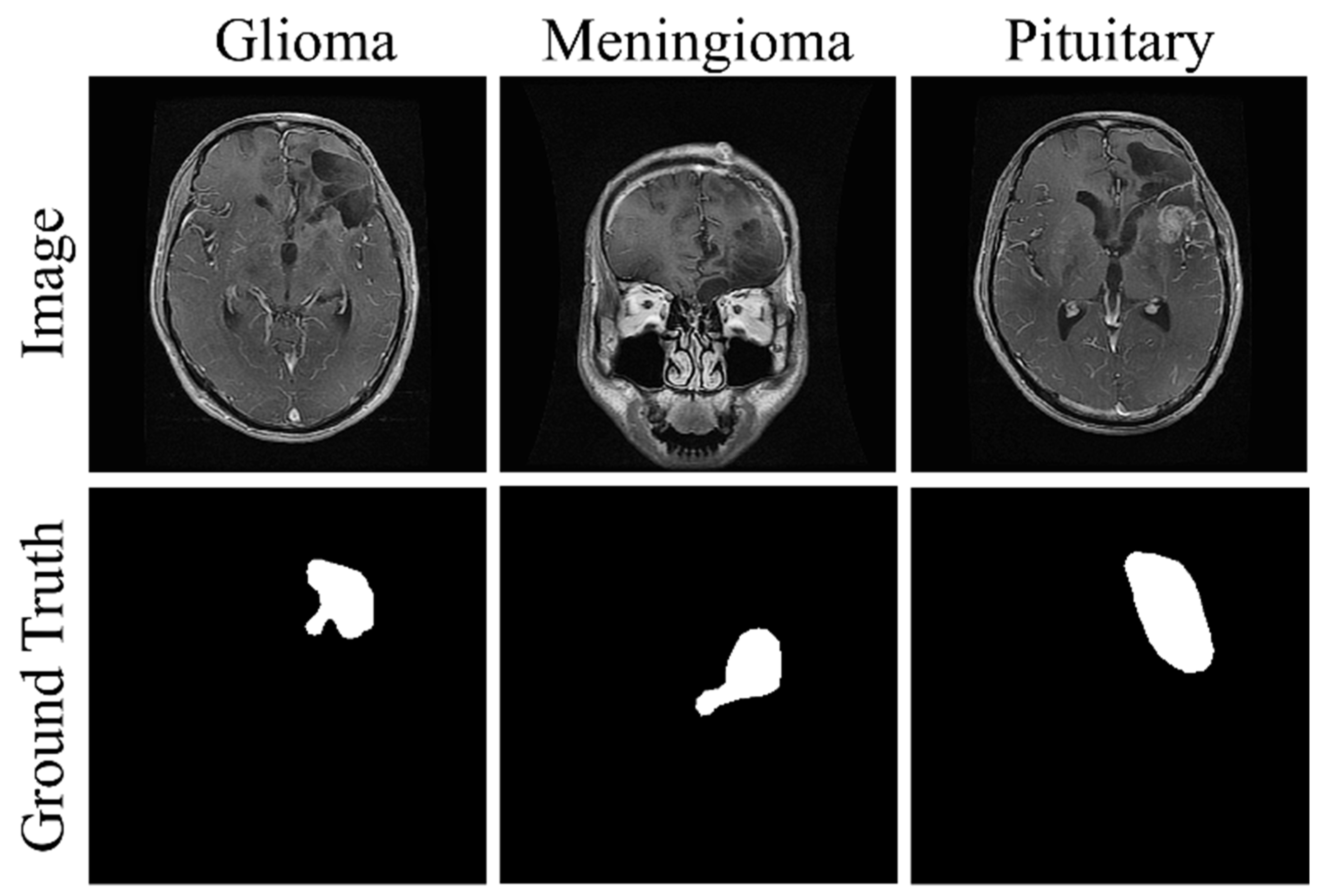
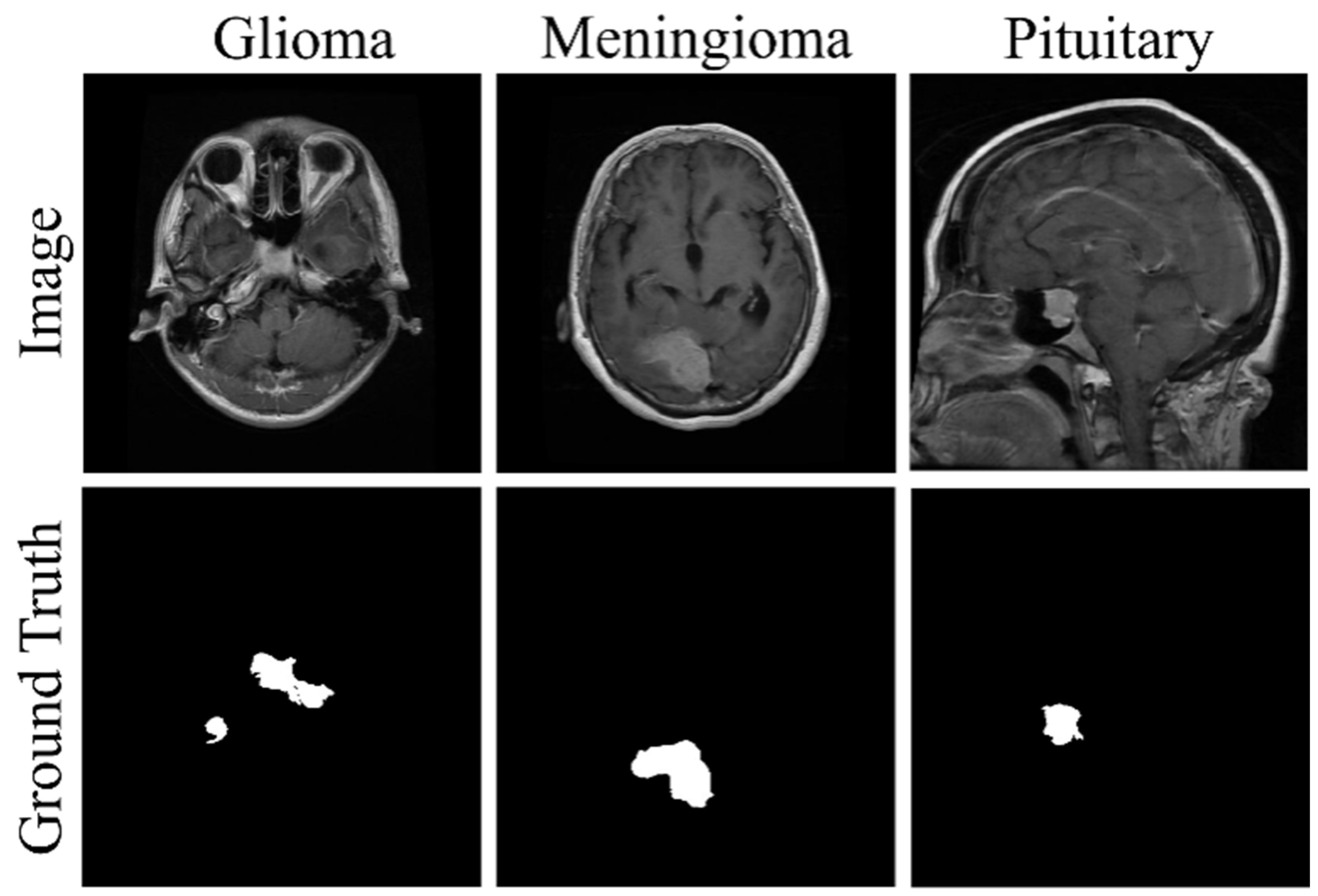
Brain Tumor Dataset: The first dataset used in this study was the publicly available Brain Tumor Dataset: Segmentation & Classification, released by Indrakumar K on Kaggle. This derivative repository was assembled from the four-class Brain Tumor MRI Dataset on Kaggle and the contrast-enhanced MRI dataset developed by Cheng et al. and distributed through SciDB v1 and Figshare v8 [36]. The former mainly provides image-level diagnostic labels, whereas the pixel-level annotations used in this study were not generated by the authors of the present work or inferred from the classification labels. Instead, they originate from the Cheng dataset, which provides manually delineated tumor contours and corresponding binary tumor masks. The associated study reports that the tumor boundaries were manually delineated by three experienced radiologists for 3064 T1-weighted contrast-enhanced MRI slices collected from 233 patients. The derivative segmentation subset used in our experiments contains 2192 two-dimensional MRI image–mask pairs, comprising 554 glioma, 708 meningioma, and 930 pituitary tumor images. Only one final mask is publicly available for each image. According to the repository description, intensity normalization to the range of 0 to 1, Gaussian filtering, and contrast enhancement were applied during dataset preparation. In our experiments, all images and masks were resized to 224 × 224 pixels and randomly divided into training and test sets at a ratio of 8:2 using a random seed of 42. Representative images and their corresponding ground-truth masks are shown in Figure 4.

BRICS 2025: The second dataset used in this study was BRISC 2025, where BRISC denotes Brain tumor Image Segmentation and Classification [37]. It is a curated dataset designed for brain tumor MRI segmentation and classification. The complete classification dataset contains 6000 two-dimensional, single-slice, contrast-enhanced T1-weighted MRI images, including 5000 training images and 1000 test images across four diagnostic categories: glioma, meningioma, pituitary tumor, and non-tumorous cases. For the segmentation experiments, only the official segmentation subset was used. This subset contains 4793 MRI image–mask pairs from the three tumor categories, including 3933 training pairs and 860 test pairs.

The segmentation masks were created using AnyLabeling and iteratively refined by a trained annotation team. The masks and class labels were subsequently verified under the supervision of a certified radiologist and physician, and disagreements were resolved collaboratively through visual comparison and overlap inspection. The images cover the axial, coronal, and sagittal planes, and their class and plane distributions are summarized in

Table 2. Class distribution of the training and test sets in the BRICS 2025 Dataset.

Class	Train			Test
	Axial	Coronal	Sagittal	Axial	Coronal	Sagittal
Glioma	347	428	372	85	81	88
Meningioma	423	426	480	134	89	83
Pituitary	428	496	533	116	98	86
Non-tumorous	352	310	405	52	48	40
Total	5000			1000

. Representative images and corresponding ground-truth masks are shown in Figure 5.

4.2. Loss Function

To achieve both pixel-level classification accuracy and region-level shape consistency in the tumor segmentation task, this study adopts a hybrid loss function strategy. This strategy combines distribution-driven and region-driven loss functions to address class imbalance and improve boundary segmentation accuracy. Specifically, we use the widely adopted ${\mathcal{L}}_{\mathrm{C}\mathrm{E}}$ and ${\mathcal{L}}_{\mathrm{D}\mathrm{i}\mathrm{c}\mathrm{e}}$ in this field. The corresponding formulas are given as follows (Equations (18) and (19)).

$${\mathcal{L}}_{CE}=-{\displaystyle \frac{1}{N}}{\displaystyle \sum _{i=1}^N}{\displaystyle \sum _{c=1}^C}{y}_{i,c}log\left(p_{i,c}\right)$$

(18)

$${\mathcal{L}}_{Dice}=1-{\displaystyle \frac{1}{C}}{\displaystyle \sum _{c=1}^C}{\displaystyle \frac{2{\displaystyle {\sum }_{i=1}^N}{p}_{i,c}{y}_{i,c}+\epsilon }{{\displaystyle {\sum }_{i=1}^N}{p}_{i,c}+{\displaystyle {\sum }_{i=1}^N}{y}_{i,c}+\epsilon }}$$

(19)

Here, $C$ denotes the number of classes, $N$ denotes the total number of pixels, and $\epsilon$ denotes the smoothing coefficient. $p_{i,c}$ represents the predicted probability that the ith pixel belongs to class $c$, while $y_{i,c}$ represents the encoded ground-truth label.

4.3. Evaluation Metrics

The comparative evaluation in our experiments was conducted using a series of metrics based on the confusion matrix. TP refers to the cases in which the model correctly predicts positive samples as positive. FP refers to the cases in which the model incorrectly predicts negative samples as positive. TN refers to the cases in which the model correctly predicts negative samples as negative. FN refers to the cases in which the model incorrectly predicts positive samples as negative.

Specifically, Accuracy (Acc), Precision (Pre), Recall, F1-score, Dice Coefficient, and Intersection over Union (IoU) were adopted in this study. Larger values of these metrics indicate better model performance. Through the collaborative evaluation of multiple metrics, the clinical applicability of the model can be quantified objectively and comprehensively. The corresponding formulas are given as follows.

$$Accuracy={\displaystyle \frac{TP+TN}{TP+TN+FP+FN}}$$

(20)

Accuracy (Equation (20)) represents the proportion of correctly predicted samples among all samples. It measures the consistency between the predicted mask and the ground-truth mask over the entire image from the most intuitive perspective.

$$Precision={\displaystyle \frac{TP}{TP+FP}}$$

(21)

Precision (Equation (21)) represents the proportion of actual positive samples among all samples predicted as positive by the model. It evaluates the anti-interference capability of the model and quantifies its ability to suppress false alarms in normal tissues.

$$Recall={\displaystyle \frac{TP}{TP+FN}}$$

(22)

Recall (Equation (22)) represents the proportion of all real positive samples that are correctly identified by the model. It evaluates the detection capability of the model from a safety perspective and ensures that lesion regions are not missed.

$$F1-Score={\displaystyle \frac{2TP}{2TP+FP+FN}}$$

(23)

F1-Score (Equation (23)) is the harmonic mean of Precision and Recall and is used to comprehensively evaluate both the Precision and Recall of the model. In class imbalance scenarios, it is usually more informative than Accuracy because it considers both false detections and missed detections.

$$Dice={\displaystyle \frac{2TP}{2TP+FP+FN}}$$

(24)

The Dice coefficient (Equation (24)) is commonly used in image segmentation tasks to measure the degree of overlap between the predicted region and the ground-truth annotation region. In binary segmentation tasks, Dice has the same mathematical form as F1-score. It can be regarded as the F1-score in segmentation tasks and focuses on measuring the similarity between the predicted region and the real region.

$$IoU={\displaystyle \frac{TP}{TP+FP+FN}}$$

(25)

IoU (Equation (25)) represents the ratio of the intersection between the predicted positive region and the real positive region to their union.

$$mIoU={\displaystyle \frac{1}{N}}{\displaystyle \sum _{i=1}^N}{IoU}_i$$

(26)

mIoU (Equation (26)) is a commonly used comprehensive evaluation metric in multi class segmentation tasks. It represents the average IoU across all classes and can comprehensively reflect the segmentation performance of the model for different categories. Therefore, it is more suitable for evaluating the overall segmentation quality in multi class tasks.

4.4. Baseline Models

For comparison, we adopted the classic U-Net architecture [10], which was selected because it is widely used as a general benchmark in the field of image segmentation. In addition, Attention U-Net [17], SLf-UNet [35], CENet [38], TransUNet [19], UNet3+ [39], VM-UNet [40], and DeepLabV3+ [41] were used as other baseline methods for direct comparison. All methods were evaluated under the same hyperparameter settings to ensure the fairness and objectivity of the experimental results.

4.5. Implementation Details

All experiments were implemented using Python v3.10 and the PyTorch v2.1.2 framework with CUDA v11.8 acceleration. The experiments were conducted on a workstation equipped with an Intel Xeon E5 2667 v4 processor and an NVIDIA GeForce RTX 3060 Ti graphics card. The processor and graphics card were manufactured by Intel Corporation (Santa Clara, CA, USA) and NVIDIA Corporation (Santa Clara, CA, USA), respectively. The input image resolution was uniformly resized to 224 × 224. The batch size was set to 8, and all models were trained for 100 epochs. The SGD optimizer was adopted for model optimization. The initial learning rate was set to 0.01, the momentum was set to 0.9, and the weight decay was set to 1 × 10⁻⁴. A learning rate scheduler with a warm-up stage was used during training.

4.6. Experimental Results on Brain Tumor Dataset

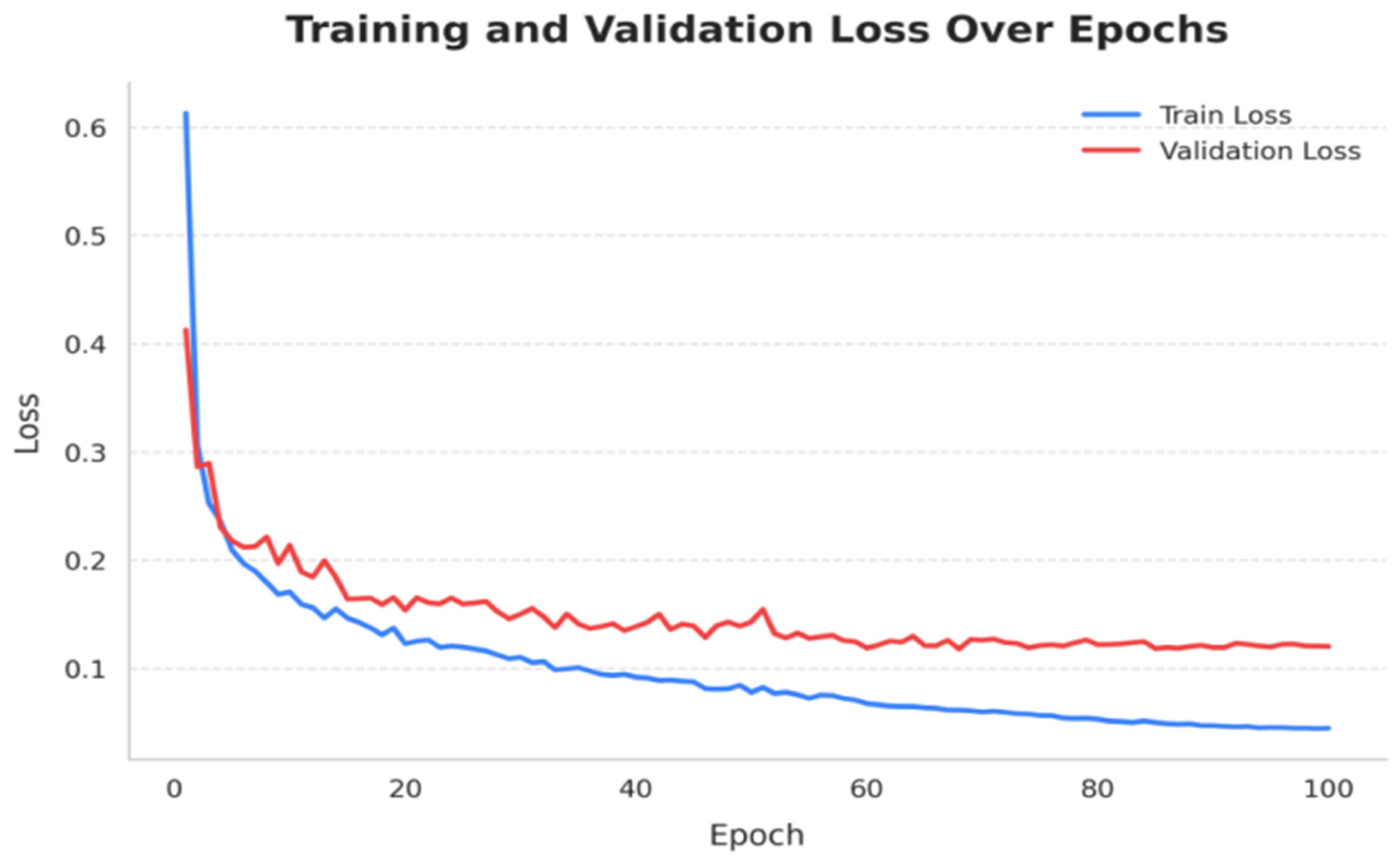
The model was trained on the Brain Tumor Dataset for a total of 100 epochs. As shown in Figure 6, the loss curves of the training set and validation set present a clear convergence trend. The losses decrease rapidly in the early training stage and become stable in the later stage without obvious divergence or abnormal oscillation. After 80 epochs, both curves tend to stabilize, and the numerical changes in the loss functions follow a reasonable pattern. These results indicate that the model achieves effective convergence during training.

As shown in

Table 3. Comparison with other studies on the Brain Tumor Dataset.

Methods	mIoU	Acc	Recall	Pre	F1	Dice
Attention U-Net [17]	84.605%	99.416%	84.474%	80.076%	82.216%	0.796
SLf-UNet [35]	85.372%	99.395%	84.208%	78.251%	81.598%	0.742
CENet [38]	80.863%	99.261%	81.348%	72.919%	76.903%	0.740
DeepLabV3+ [41]	85.074%	99.423%	82.971%	82.746%	82.858%	0.800
TransUNet [19]	81.965%	99.323%	84.416%	73.368%	78.505%	0.753
U-Net [10]	85.228%	99.453%	86.933%	79.496%	83.048%	0.796
UNet3+ [39]	81.638%	99.285%	80.928%	75.367%	78.049%	0.740
VM-UNet [40]	76.788%	99.111%	79.978%	63.077%	70.529%	0.627
TSF U-Net	86.471%	99.499%	87.424%	82.127%	84.693%	0.819

, detailed comparative experiments were conducted between the proposed model and various mainstream models. The bolded values indicate the best results. U-Net achieves an mIoU of 85.228% and a Dice coefficient of 0.796 through its classical encoder–decoder structure and skip connections, forming a strong baseline. Although Attention U-Net introduces gated attention into skip connections to suppress irrelevant backgrounds, its mIoU slightly decreases to 84.605%, indicating that simple spatial attention does not fully exploit the guiding potential of deep semantics for shallow features. DeepLabV3+ captures multi-scale context through the ASPP module and obtains the highest precision. However, its continuous downsampling and atrous convolution tend to lose tumor boundary details, resulting in a recall of only 82.971%. TransUNet embeds a Transformer encoder into the U-shaped structure and uses self-attention to model global dependencies, increasing the recall to 84.416%. However, the global receptive field also introduces a large amount of background interference, causing the precision to decrease to 73.368% and the Dice coefficient to only 0.753. UNet3+ adopts full-scale skip connections to fuse multi-level features, but this may lead to information redundancy and noise accumulation, with a recall of only 80.928% and an mIoU of 81.638%. VM-UNet performs long-range modeling based on the visual state space model SS2D, but it shows the weakest performance in this task because of its insufficient ability to preserve fine local spatial details.

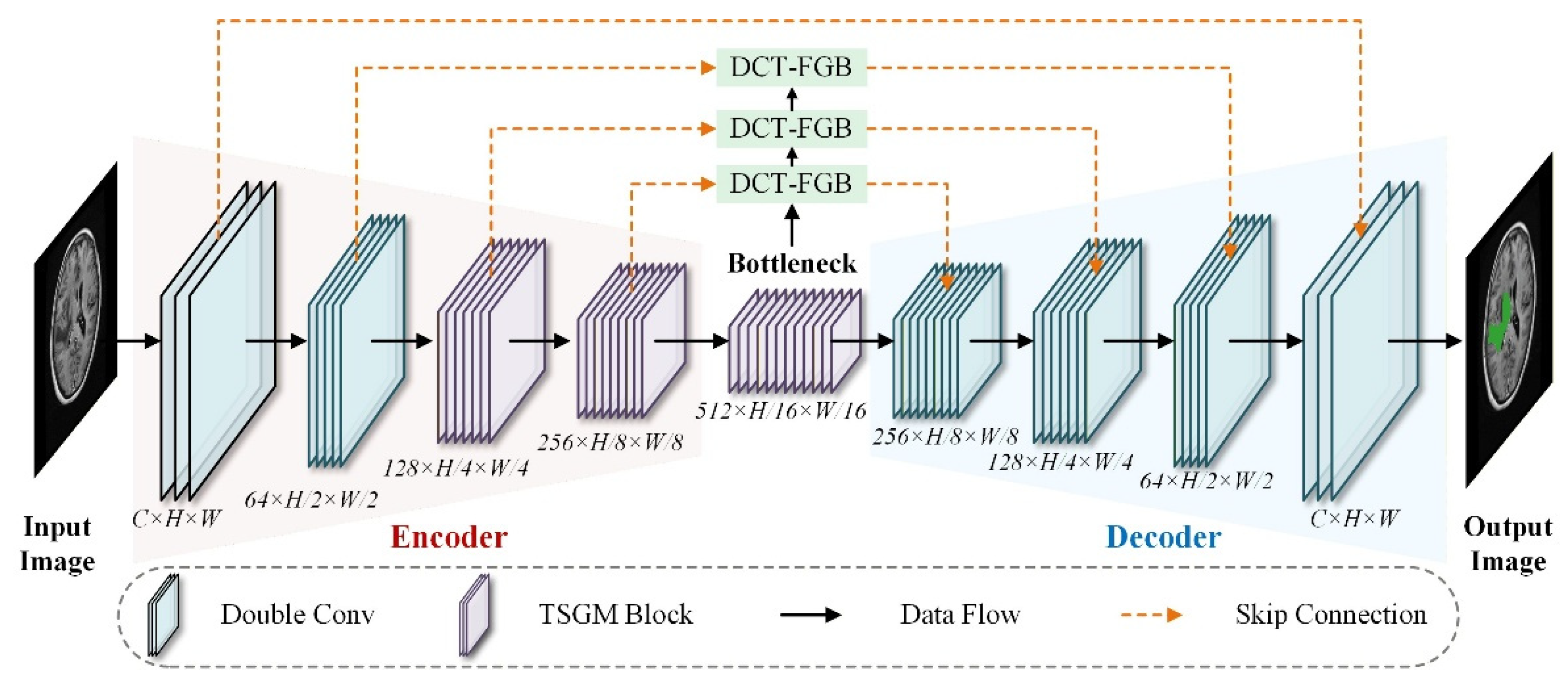
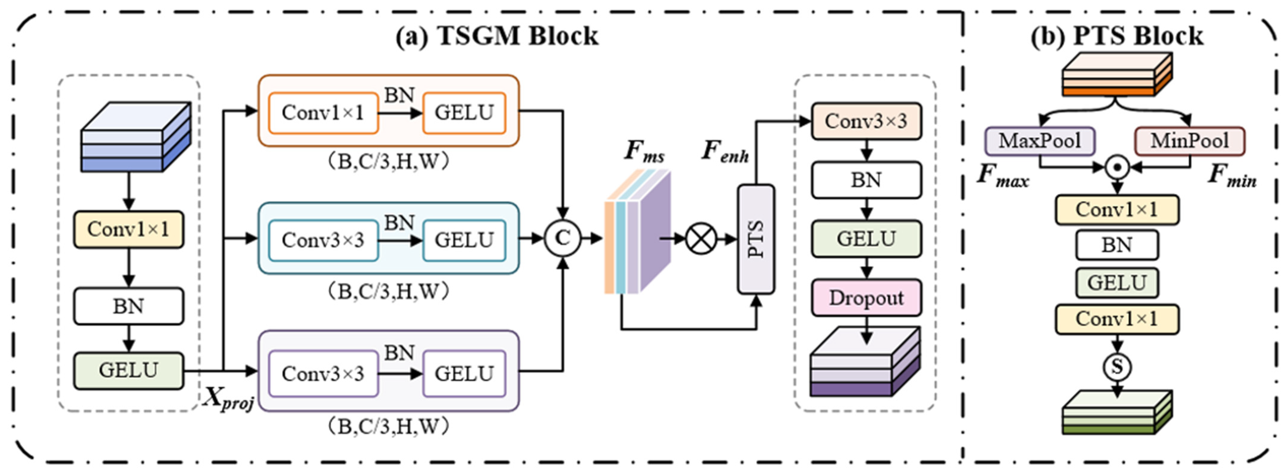
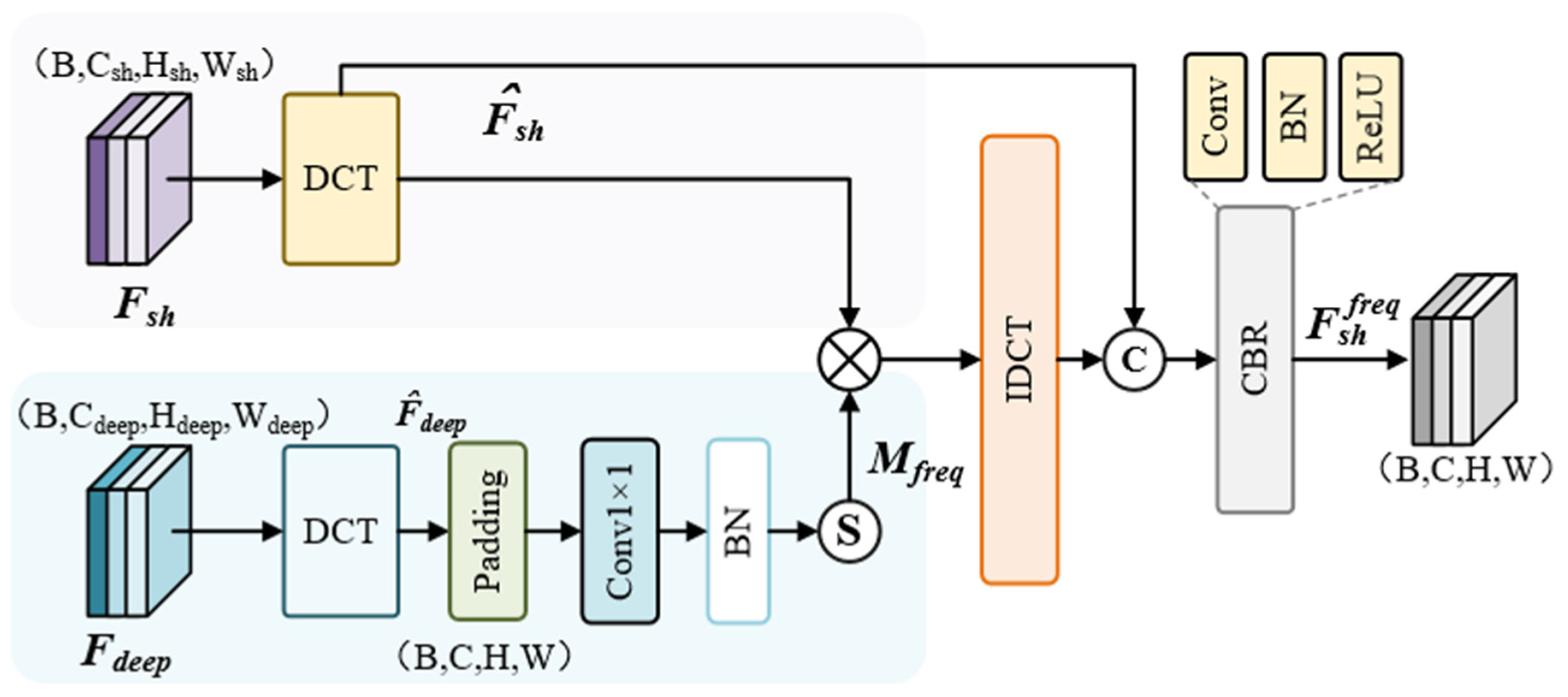
To further clarify the methodological differences from the most closely related architectures, Attention U-Net and SLf-UNet were examined as representative attention-based and frequency-based variants, respectively. Attention U-Net uses coarse decoder semantics to gate fine encoder features in skip connections, thereby realizing implicit cross-scale feature selection. However, it lacks explicit receptive field adaptation and direct modeling of local texture transitions. In contrast, TSGM combines parallel convolutional branches with different receptive fields and texture-span gating in the encoder, enabling TSF U-Net to jointly characterize tumor morphology, heterogeneous textures, and boundary transitions. Consequently, TSF U-Net surpasses Attention U-Net by 1.866, 2.950, 2.051, and 2.477 percentage points in mIoU, Recall, Precision, and F1-score, respectively, while increasing the Dice coefficient by 0.023. SLf-UNet combines spatial features with low-frequency representations and performs upsampling through frequency-domain zero padding, with an emphasis on global structural information. In comparison, DCT-FGB uses aligned deep spectral features to generate gating masks that adaptively calibrate the shallow spectrum in each skip connection, followed by inverse transformation and residual spatial fusion. This semantically guided spectral filtering reduces irrelevant frequency responses while preserving useful spatial details. Compared with SLf-UNet, TSF U-Net improves mIoU, Recall, Precision, and F1-score by 1.099, 3.216, 3.876, and 3.095 percentage points, respectively, and increases the Dice coefficient from 0.742 to 0.819. These results demonstrate that the coordinated modeling of multi-scale morphology, pathological texture variations, and frequency-domain feature selection provides a more balanced segmentation representation than cross-scale attention or spatial and low-frequency fusion alone.

The proposed TSF U-Net achieves an mIoU of 86.471%, a recall of 87.424%, a Dice coefficient of 0.819, and an F1-score of 84.693%, all ranking first among the compared methods. Meanwhile, its precision remains very close to that of DeepLabV3+, indicating that the model maintains a high positive predictive ability while significantly improving tumor recall. These results fully demonstrate that the multi-scale texture enhancement of TSGM and the semantic cleaning of DCT-based frequency-domain gating can form an effective complement, thereby improving the comprehensive performance of brain tumor segmentation.

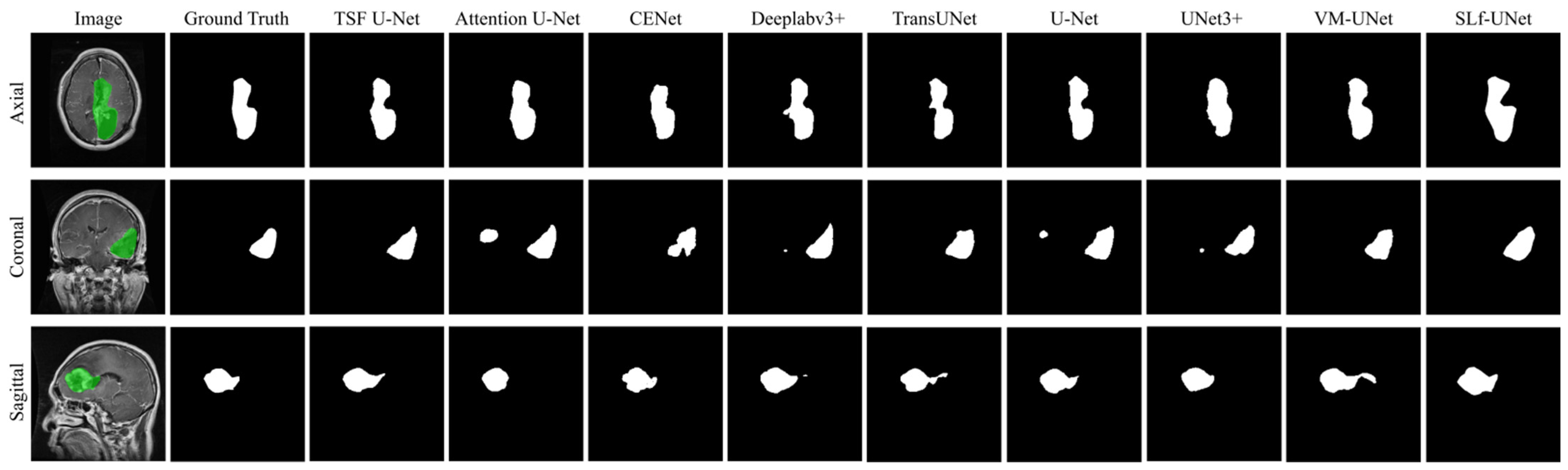
Figure 7 shows the visual segmentation results of different comparison algorithms on three different types of images in the test set. For axial images, almost all widely used U-Net-based comparison algorithms show inaccurate and unclear tumor boundaries. For coronal images, Attention U-Net, U-Net, and UNet3+ show obvious missegmentation, indicating a relatively high false-positive rate. For sagittal images, Attention U-Net, TransUNet, and VM-UNet produce obvious morphological misjudgments. In contrast, the proposed model effectively avoids these over-segmentation and missegmentation problems, and its predicted regions are closer to the real tumor morphology and boundaries. This further demonstrates that our model achieves better segmentation performance.

Furthermore, we perform comprehensive quantitative evaluations of the computational efficiency for all competing models as well as our proposed model. All the results are summarized in

Table 4. Comparison of network complexity with other models.

Methods	Params (M)	FLOPs (G)	Latency (ms)	FPS
Attention U-Net [17]	34.879	101.729	14.406	69.418
SLf-UNet [35]	32.584	58.422	26.203	85.521
CENet [38]	33.371	25.134	50.796	19.687
DeepLabV3+ [41]	27.229	17.860	9.832	101.712
TransUNet [19]	109.243	83.832	29.158	34.296
U-Net [10]	17.263	61.226	8.304	120.429
UNet3+ [39]	33.005	60.171	16.693	59.906
VM-UNet [40]	38.295	12.709	28.259	35.387
TSF U-Net	27.926	93.931	15.031	66.528

. The computational efficiency results show that TSF U-Net contains 27.926 M parameters and requires 93.931 G FLOPs, with an inference latency of 15.031 ms and a throughput of 66.528 FPS. Compared with the original U-Net, the proposed model increases the parameter count and FLOPs by 10.663 M and 32.705 G, corresponding to increases of 61.77% and 53.42%, respectively. Its inference latency increases by 6.727 ms, while the FPS decreases by 44.76%. This additional cost is mainly associated with the parallel multi-scale convolutional branches of TSGM and the frequency-domain feature processing performed by DCT-FGB.

Nevertheless, TSF U-Net has fewer parameters than Attention U-Net, CENet, TransUNet, UNet3+, VM-UNet and SLf-UNet, and achieves lower latency than SLf-UNet, CCENet TransUNet, UNet3+, and VM-UNet. Although its FLOPs are relatively high, the model maintains a throughput of 66.528 FPS under the adopted experimental conditions. These results indicate that the improvements in segmentation performance are accompanied by a measurable computational cost, while the overall parameter scale and inference efficiency remain competitive with those of several comparison models.

4.7. Experimental Results on BRICS 2025 Dataset

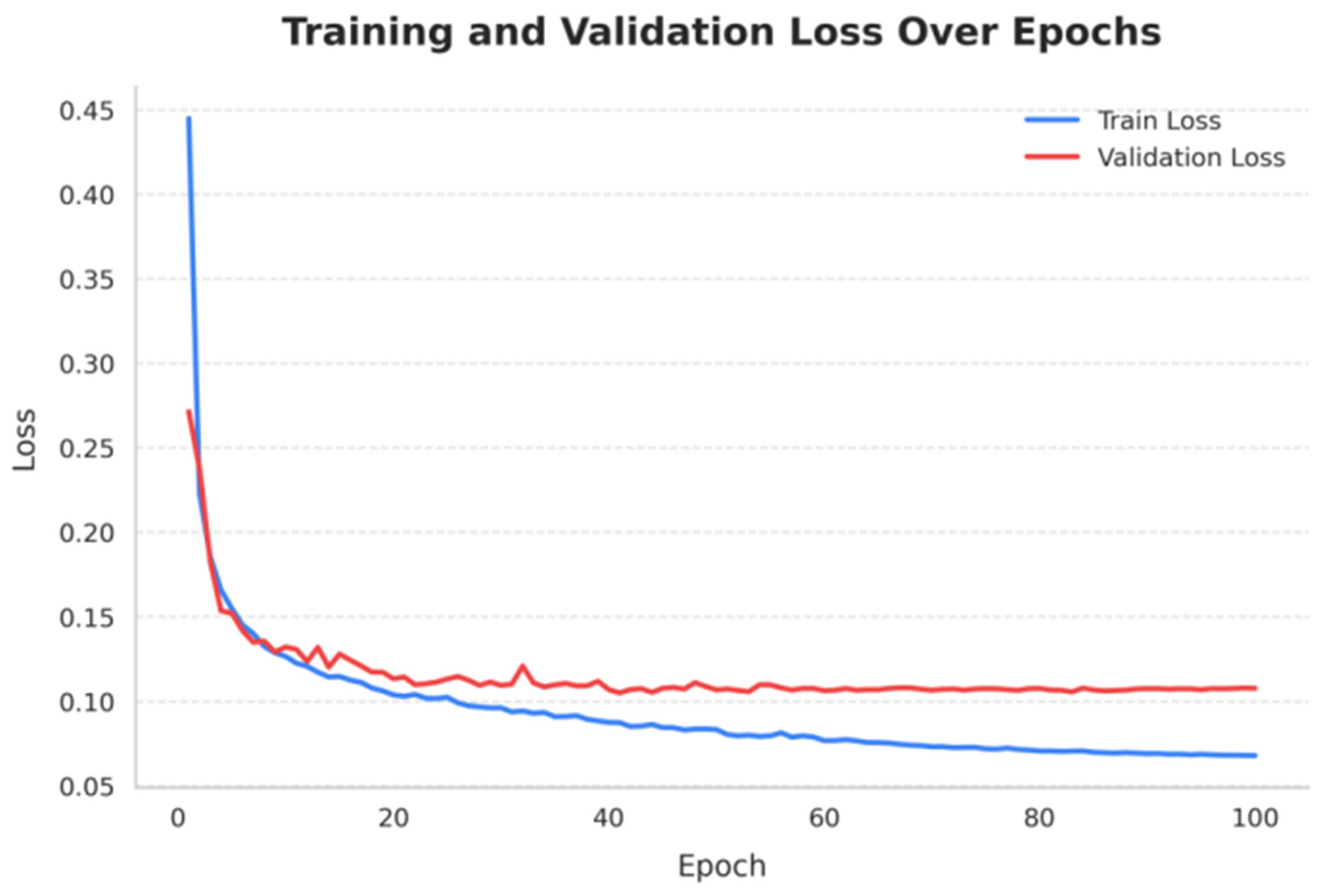
The model was also trained on this dataset for 100 epochs. As shown in Figure 8, both the training and validation loss curves show a clear downward trend. The training loss decreases from 0.445 to 0.068, with a reduction of approximately 84.7%, while the validation loss decreases from 0.271 to 0.108, with a reduction of approximately 60.3%. The two curves exhibit rapid decline in the early stage, smooth transition in the middle stage, and convergence to low values in the later stage. The training loss remains lower than the validation loss with a stable gap, and no obvious divergence or continuous increase in validation loss is observed. These results indicate that the model has stable optimization, favorable convergence, no obvious overfitting, and reliable generalization ability on this dataset.

Similar to the experiments on the Brain Tumor Dataset, the proposed model and other comparison models were trained on the BRICS 2025 Dataset, and the corresponding image segmentation results were obtained. The bolded values indicate the best results. As shown in

Table 5. Comparison with other studies on the BRICS 2025 Dataset.

Methods	mIoU	Acc	Recall	Pre	F1	Dice
Attention U-Net [17]	88.737%	99.494%	91.023%	84.488%	87.634%	0.840
SLf-UNet [35]	88.358%	99.491%	89.251%	82.729%	86.589%	0.828
CENet [38]	87.182%	99.413%	88.783%	82.805%	85.690%	0.819
DeepLabV3+ [41]	88.536%	99.475%	89.160%	85.692%	87.391%	0.834
TransUNet [19]	88.140%	99.465%	90.391%	83.658%	86.894%	0.830
U-Net [10]	88.852%	99.498%	90.840%	84.911%	87.776%	0.838
UNet3+ [39]	87.487%	99.425%	88.559%	83.732%	86.078%	0.820
VM-UNet [40]	86.404%	99.366%	86.846%	82.647%	84.695%	0.798
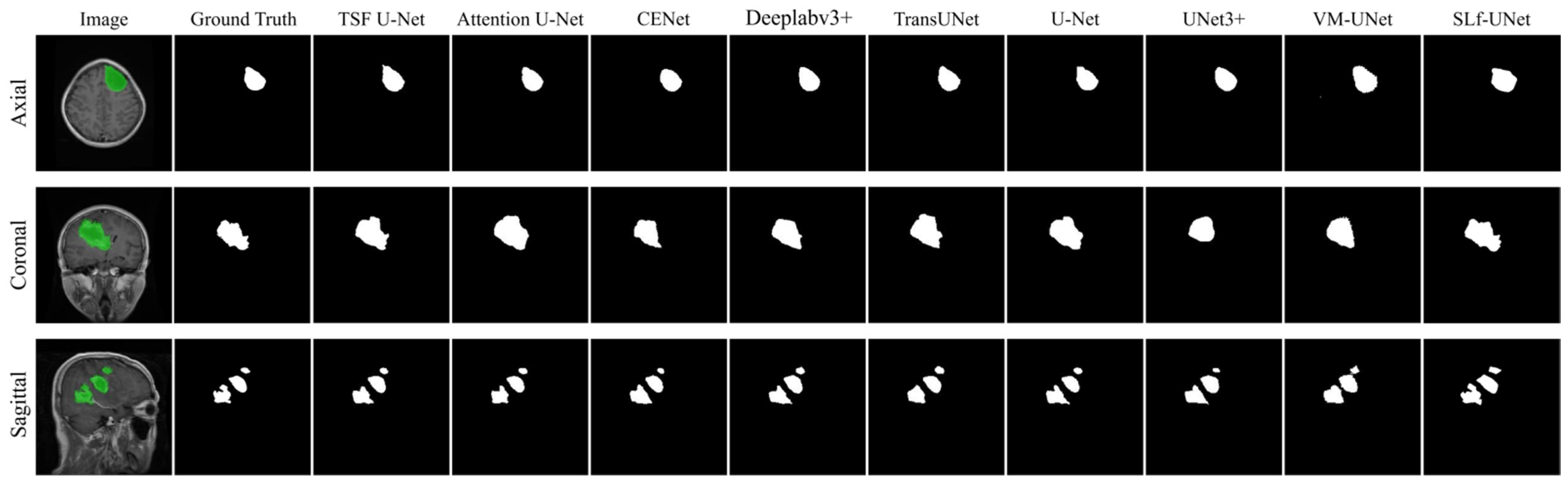
TSF U-Net	88.882%	99.495%	90.029%	85.708%	87.816%	0.838

, the proposed model achieves the best performance in mIoU, Acc, Precision, and F1-score, with only Recall and Dice being slightly lower than those of Attention U-Net. In the visual comparison of image segmentation shown in Figure 9, it can be intuitively observed that the proposed model identifies tumor regions and boundaries more accurately. The experimental results on BRICS 2025 demonstrate that the proposed model has favorable generalization ability and robustness. Compared with SLf-UNet, which mainly enhances global structural representation by combining spatial and low-frequency features, TSF U-Net further integrates explicit multi-scale texture modeling through TSGM and semantic-guided spectral calibration through DCT-FGB. This design strengthens boundary-related local variations while suppressing irrelevant shallow frequency responses. TSF U-Net outperforms SLf-UNet on every evaluation metric. These results indicate that the collaboration between spatial texture enhancement and adaptive frequency selection provides more balanced segmentation performance on the BRICS 2025 Dataset.

It should be noted that TSF U-Net achieves a Recall of 90.029%, which is 0.994, 0.362, and 0.811 percentage points lower than those of Attention U-Net, TransUNet, and U-Net, respectively. This difference may be attributed to the relatively conservative feature selection of the proposed model. TSGM provides less additional enhancement to low-contrast or blurred-boundary regions with limited local texture spans, while the deep semantic guidance in DCT-FGB may reduce the influence of weak tumor responses during frequency-domain feature selection. These mechanisms suppress false positives but may introduce a small increase in false negatives. In contrast, direct skip connections, spatial attention, and global self-attention may preserve a broader range of weak positive responses. Nevertheless, the Precision of TSF U-Net is 1.220, 2.050, and 0.797 percentage points higher than those of the three comparison models, respectively, while its mIoU and F1-score are also higher. The lower Recall therefore mainly reflects a tradeoff between Precision and Recall. Recall-sensitive loss functions and adaptive feature guidance will be investigated to reduce missed low-contrast tumor regions.

4.8. Ablation Study

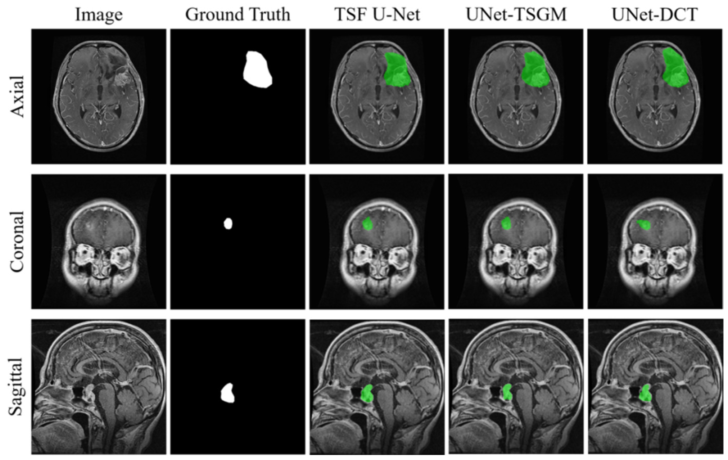
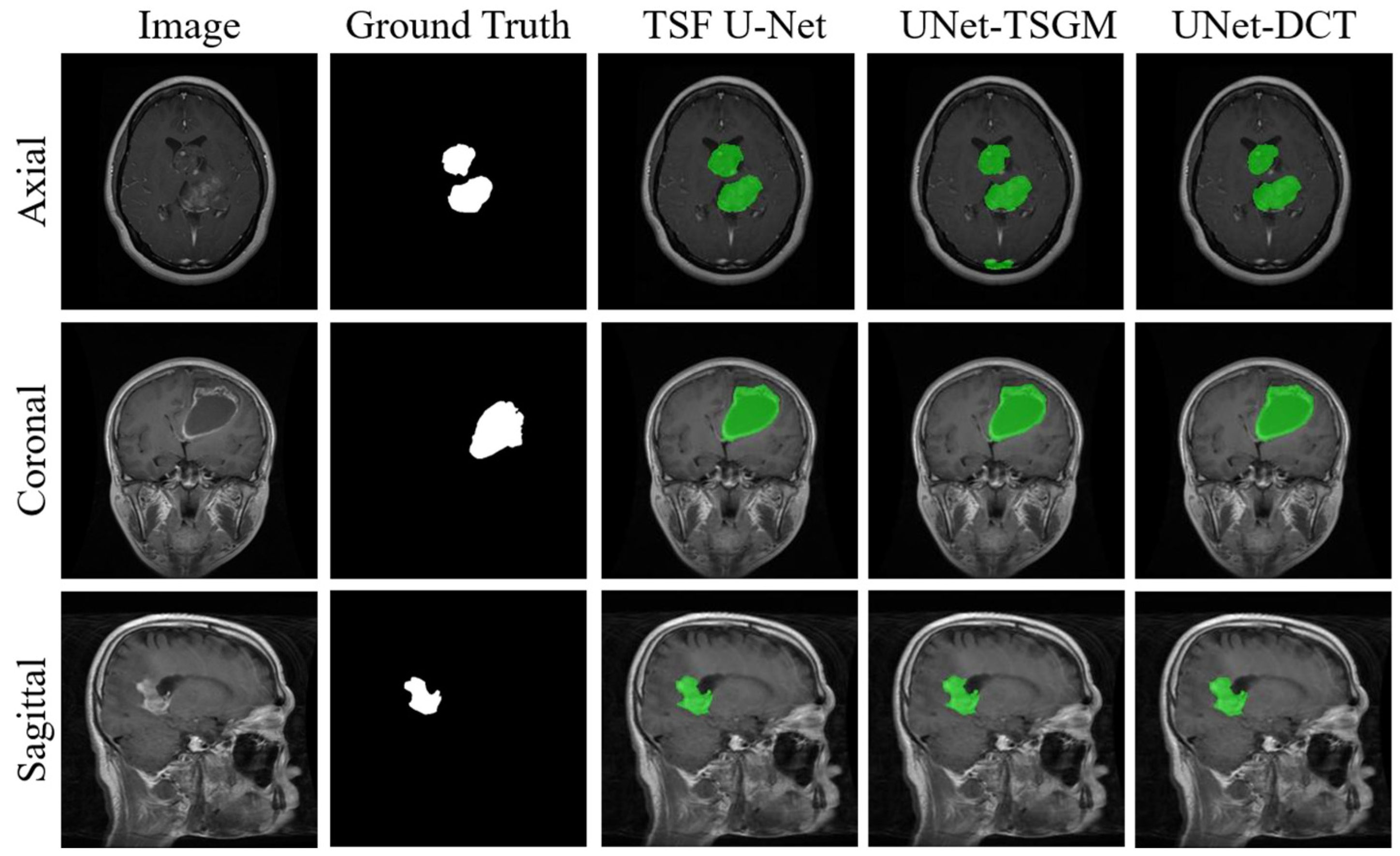
To evaluate the individual and joint contributions of the proposed modules, ablation experiments were conducted on the Brain Tumor and BRICS 2025 datasets. Four configurations were compared: the U-Net baseline, the TSGM variant, the DCT-FGB variant, and the complete TSF U-Net. Their quantitative results are reported in Table 5 and

Table 6. Ablation study results on the Brain Tumor Dataset.

Methods	mIoU	Acc	Recall	Pre	F1	Dice
U-Net [10]	85.228%	99.453%	86.933%	79.496%	83.048%	0.796
UNet-DCT	85.809%	99.467%	85.854%	81.894%	83.827%	0.814
UNet-TSGM	86.077%	99.487%	87.611%	81.000%	84.176%	0.798
TSF U-Net	86.471%	99.499%	87.424%	82.127%	84.693%	0.819

, while representative segmentation results are shown in Figure 10 and Figure 11. The following analysis discusses the limitations of the baseline and the effects of each module.

The baseline model adopts the classical U-Net encoder–decoder architecture. As shown in Table 6, all evaluation results of the U-Net baseline model are lower than those of the other ablation models. The bolded values indicate the best results. Although its Accuracy reaches 99.453%, its Precision is only 79.496% and its Recall is 86.933%. This indicates that the standard U-Net can identify most lesion regions, but it still produces many false-positive predictions. This problem is particularly obvious at the junctions between lesion boundaries and complex textures, where the feature representation lacks targeted boundary enhancement and noise suppression mechanisms. Similar limitations are observed on the BRISC 2025 Dataset. As shown in

Table 7. Ablation study results on the BRICS 2025 Dataset.

Methods	mIoU	Acc	Recall	Pre	F1	Dice
U-Net [10]	88.833%	99.499%	91.162%	84.587%	87.752%	0.838
UNet-DCT	88.891%	99.496%	90.109%	85.658%	87.827%	0.839
UNet-TSGM	88.879%	99.497%	90.384%	85.380%	87.811%	0.842
TSF U-Net	89.055%	99.507%	90.749%	85.462%	88.026%	0.846

, the U-Net baseline achieves the highest Recall of 91.162% among the ablation variants, but obtains the lowest mIoU, Precision, F1-score, and Dice values of 88.833%, 84.587%, 87.752%, and 0.838, respectively. These results indicate that the direct transmission of shallow features enables U-Net to retain a broader range of potential tumor responses, but also introduces background interference and false-positive predictions, thereby limiting the accuracy of tumor boundaries and regional overlap. The results on both datasets therefore consistently demonstrate the limitations of the baseline model in discriminative feature selection and noise suppression.

Effect of TSGM Block: On the Brain Tumor Dataset, compared with the baseline model, the TSGM variant achieves a substantial improvement of 1.504% in Precision, a slight increase of 0.002% in Dice, and simultaneous improvements in mIoU and F1-score. This improvement benefits from the adaptive receptive field coverage enabled by the parallel multi-branch structure, which allows the model to focus on both small-scale details and large-scale structural information. The pathological texture-span sensor (PTS) strengthens the responses of transition regions between pathological tissues and normal tissues through texture-span attention, effectively suppressing false activations of background and irrelevant tissues. Meanwhile, the Recall is also improved by 0.678%, indicating that the overall segmentation quality is significantly enhanced. On the BRICS 2025 Dataset, the TSGM variant improves Precision, mIoU, and F1-score by 0.793%, 0.046%, and 0.059%, respectively, and increases the Dice coefficient from 0.838 to 0.842. However, its Recall decreases by 0.778%. This result suggests that TSGM consistently improves feature selectivity and regional overlap, although its enhancement of weak or low-contrast tumor responses may vary across datasets.

Effect of DCT-FGB Block: On the Brain Tumor Dataset, the DCT-FGB variant obtains a Recall of 85.854%, which is slightly lower than that of the baseline model. However, the other metrics, including mIoU, Accuracy, Precision, F1-score, and Dice, are all improved compared with the baseline. Through frequency-domain zero padding and gating mechanisms, DCT-FGB preserves the frequency structure of deep semantic information and uses it as guidance to clean shallow features. This process improves the reliability of shallow feature transmission and enhances the representation of true tumor-related regions, while exerting a relatively moderate suppression effect on false positives. Consistent results are obtained on the BRICS 2025 Dataset. Compared with U-Net, the DCT-FGB variant improves mIoU, Precision, and F1-score by 0.058, 1.071, and 0.075 percentage points, respectively, while the Dice coefficient increases from 0.838 to 0.839. Its Recall decreases by 1.053 percentage points, whereas Accuracy remains nearly unchanged. These results further indicate that frequency-domain semantic guidance improves the suppression of irrelevant shallow responses, but may also reduce the contribution of weak tumor features that are insufficiently represented in deep semantic features.

The TSF U-Net employs the TSGM block in the deep encoder stages and embeds DCT-FGB into all skip connections, forming a feature-learning strategy with collaborative enhancement in both the spatial and frequency domains. Specifically, the model captures local details and multi-scale contextual information of large lesion regions in the deep encoder stages, while performing lossless filtering on shallow spectra at the skip connection stage. In this way, the network obtains both boundary localization ability and semantic consistency. The experimental results show that only the Recall of the complete model is slightly lower than that of the TSGM variant by 0.19 percentage points. This may be because the DCT-FGB module suppresses some low-contrast, blurred-boundary, or diffuse lesion regions to a certain extent. Nevertheless, all other metrics are significantly improved compared with the baseline model and the single-module variants. This indicates that the complete model significantly enhances segmentation boundary accuracy by appropriately reducing the noise sensitivity of extreme recall regions, achieving a better balance between boundary misclassification suppression and regional completeness. On the BRICS 2025 Dataset, the complete TSF U-Net achieves the highest mIoU, Accuracy, F1-score, and Dice values of 89.055%, 99.507%, 88.026%, and 0.846, respectively. Compared with the baseline, it improves mIoU, Precision, and F1-score by 0.222, 0.875, and 0.274 percentage points, respectively, although Recall decreases slightly by 0.413 percentage points. More importantly, compared with the DCT-FGB-only and TSGM-only variants, the complete model improves Recall by 0.640 and 0.365 percentage points and mIoU by 0.164 and 0.176 percentage points, respectively. This demonstrates that the spatial and frequency-domain modules complement each other and partially compensate for the sensitivity reduction observed when either module is used independently. The visual results also intuitively show that the final model produces better segmentation maps than the other models, which is often of greater practical value in clinical segmentation scenarios.

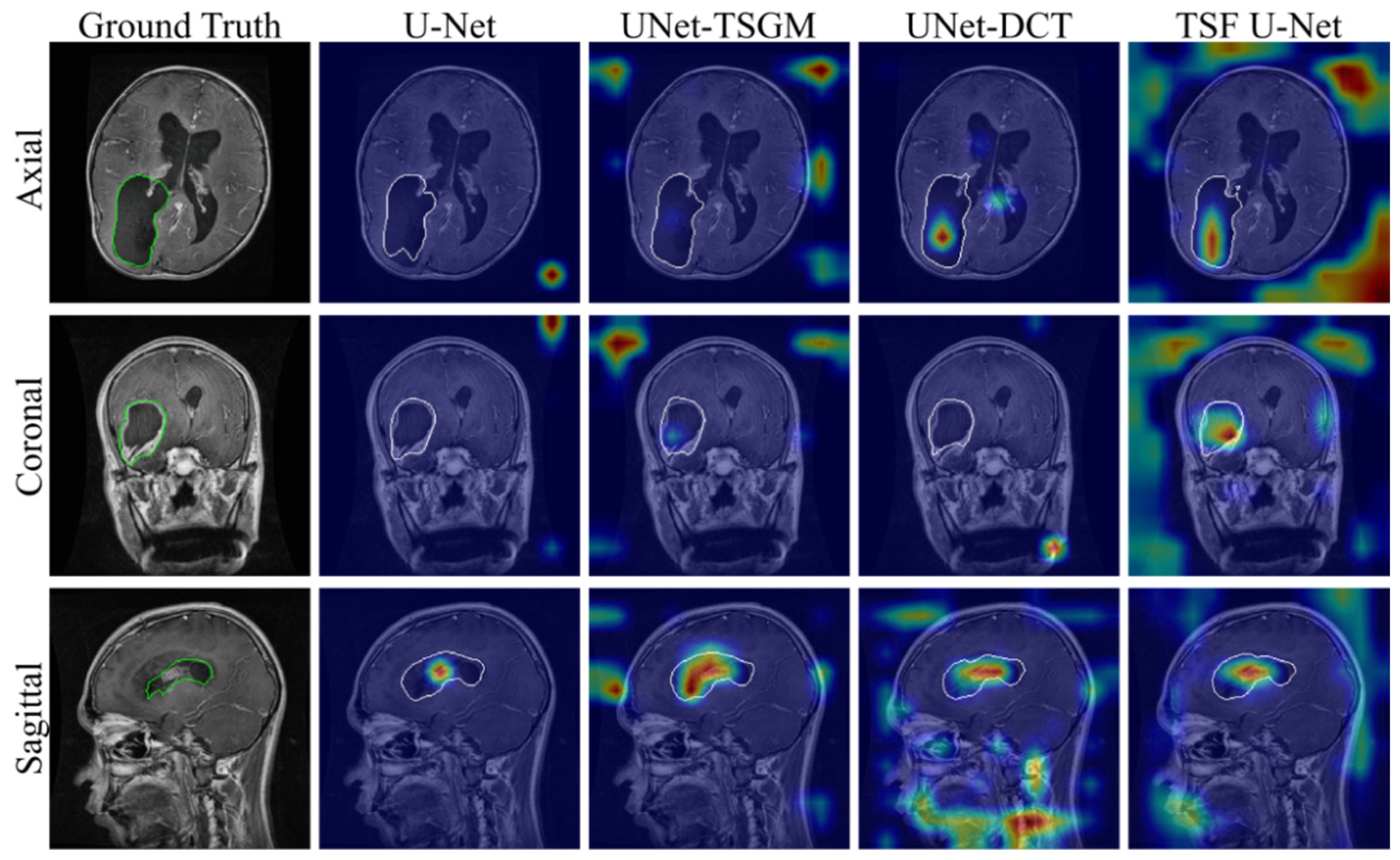
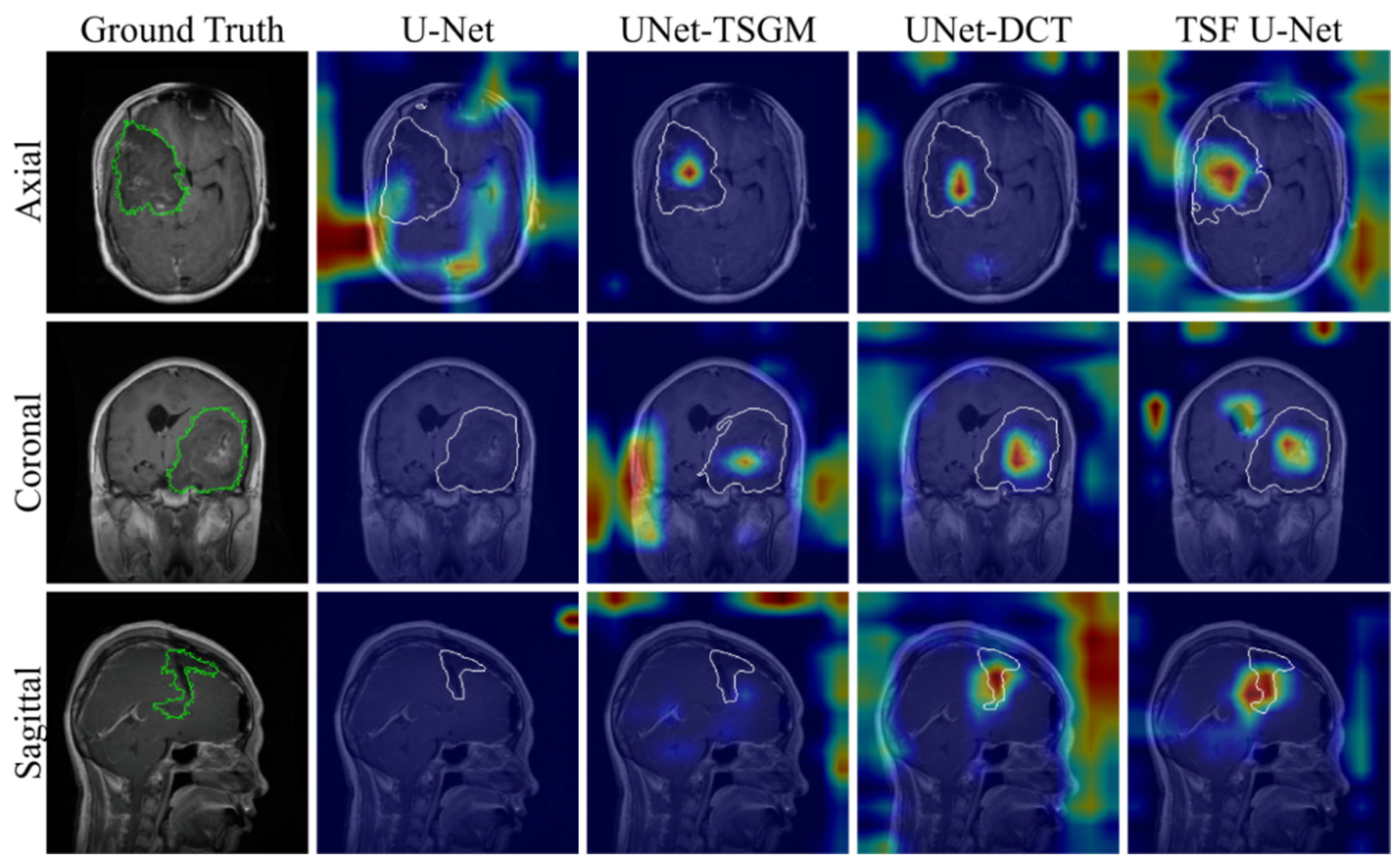
To further investigate how the proposed modules influence feature learning, feature activation maps of the ablation variants on the two datasets are visualized in Figure 12 and Figure 13. Warmer colors indicate regions receiving greater activation, while the contours denote the ground-truth tumor regions. The U-Net baseline exhibits weak or incomplete lesion responses in some cases, together with scattered activations outside the tumor regions, indicating that direct skip connections may transmit irrelevant shallow textures to the decoder. After introducing TSGM, the activation distributions are more closely aligned with heterogeneous intratumoral regions and tumor boundary transitions. This observation is consistent with the texture-span mechanism, which emphasizes regions exhibiting pronounced local feature variations. DCT-FGB further concentrates the responses in semantically relevant tumor regions and attenuates several peripheral background activations, suggesting that deep semantic frequency gating selectively filters shallow responses that are inconsistent with tumor semantics. The complete TSF U-Net generally produces more coherent activation within the annotated regions, demonstrating the complementary effects of spatial texture enhancement and frequency-domain feature selection. Nevertheless, residual extra-tumoral activations or incomplete responses at low-contrast boundaries remain in several examples, which may account for the observed tradeoff between Precision and Recall. These qualitative results provide additional evidence for the internal mechanisms and limitations of the proposed modules.

4.9. Cross-Dataset Generalization Experiment

To further evaluate the generalization ability of TSF U-Net under dataset distribution shifts, bidirectional cross-dataset experiments were conducted between the Brain Tumor Dataset and the BRISC 2025 Dataset. In each experiment, the model was trained only on the source dataset and directly evaluated on the target dataset without target-domain fine-tuning or parameter updating. The same preprocessing and evaluation settings were used to ensure that the results reflected the transferability of the learned representations rather than adaptation to the target dataset.

As shown in

Table 8. Cross-Dataset experiment results on the Brain Tumor Dataset.

Methods	mIoU	Acc	Recall	Pre	F1	Dice
Train set: Brain Tumor Test set: BRICS 2025	77.369%	98.941%	82.998%	63.015%	71.639%	0.632
Train set: BRICS 2025 Test set: Brain Tumor	70.881%	98.904%	77.973%	48.773%	60.009%	0.564

, when trained on the Brain Tumor Dataset and tested on the BRICS 2025 Dataset, TSF U-Net achieves an mIoU of 77.369%, a Recall of 82.998%, an F1-score of 71.639%, and a Dice coefficient of 0.632. These results indicate that the model retains a certain ability to identify tumor regions across datasets. However, the Precision decreases to 63.015%, suggesting that differences between the source and target distributions introduce additional false-positive predictions. In the reverse direction, training on the BRICS 2025 Dataset and testing on the Brain Tumor Dataset results in an mIoU of 70.881%, a Recall of 77.973%, a Precision of 48.773%, an F1-score of 60.009%, and a Dice coefficient of 0.564. Compared with the opposite direction, mIoU, Recall, Precision, and F1-score decrease by 6.488%, 5.025%, 14.242%, and 11.630%, respectively. This directional difference suggests that features learned from the Brain Tumor Dataset transfer more effectively to the BRICS 2025 Dataset than vice versa.

Overall, the results demonstrate that TSF U-Net retains a degree of cross-dataset transferability, while the performance degradation, particularly in Precision and Dice, reveals the continuing influence of differences in image acquisition, intensity distribution, lesion appearance, and annotation criteria. Future work will investigate domain adaptation and intensity normalization strategies to improve robustness across heterogeneous clinical datasets.

5. Conclusions

This study presents TSF U-Net, an improved U-Net architecture for brain tumor MRI segmentation. In the encoder, the proposed TSGM block combines parallel convolutional branches with different receptive fields and a pathological texture-span gating mechanism derived from local maximum and minimum feature responses. The multi-scale branches capture both local tumor details and the broader morphological context, while the texture-span gate emphasizes heterogeneous intratumoral regions and boundary transitions and suppresses homogeneous normal-tissue responses without requiring additional boundary supervision. In the skip connections, the proposed DCT-FGB block introduces a top-down semantic filtering mechanism. Deep and shallow features are mapped into the discrete cosine transform domain, where the frequency representation of deep semantic features is used to selectively calibrate shallow frequency components before decoder fusion. This process reduces the transmission of background noise and irrelevant textures while preserving tumor-related contours and structural details. Together, TSGM and DCT-FGB form a complementary spatial–frequency feature-learning framework within the classical U-Net architecture. This framework improves pathological feature representation, the reliability of shallow features, and boundary recovery. TSF U-Net achieves mIoU values of 86.471% and 88.882% on the Brain Tumor Dataset and the BRISC 2025 Dataset, respectively. The ablation experiments and activation-map analyses further confirm the contributions of the two modules to feature selectivity, boundary localization, and noise suppression.

Medical image artificial intelligence is evolving from conventional convolutional networks toward attention-based, Transformer-based, and hybrid representation frameworks. Within this development, TSF U-Net offers a targeted combination of boundary-sensitive texture modeling and semantic frequency-domain feature selection while retaining the efficient structure of U-Net. However, quantitative improvements on public datasets alone are insufficient to establish clinical utility. Clinical translation will also require standardized experimental protocols, reproducible implementations, independent external validation, interpretable predictions, and integration into radiologist-supervised workflows.

The current study is limited to two public two-dimensional datasets and has not yet included independent multi-center clinical data. Nevertheless, without target-domain fine-tuning, TSF U-Net achieves mIoU values of 77.369% and 70.881% in the two cross-dataset transfer directions, providing initial evidence of its ability to retain tumor-related representations under distribution shifts. The accompanying reductions in Precision and Dice indicate that differences in image acquisition, intensity distributions, and annotation criteria still affect model robustness. Future work will therefore focus on multi-center and multi-vendor validation, domain adaptation, intensity harmonization, and three-dimensional modeling. Uncertainty estimation and prospective clinical evaluation will also be investigated to improve generalization while preserving the model’s advantages in boundary perception and noise suppression.