Towards Probabilistic and Risk-Aware Active Disturbance Rejection Control: Particle-Filter-Based Extended-State Estimation and Control Action Selection

Abstract

This paper proposes a novel probabilistic approach to Active Disturbance Rejection Control (ADRC) based on particle filtering (PF) for extended-state estimation. Unlike the classical Extended State Observer (ESO), the proposed method represents the system state and total disturbance using weighted particles, enabling the direct incorporation of non-Gaussian noise and model uncertainty. The PF-based estimator is integrated within the ADRC framework and compared with conventional ESO- and Kalman filter-based approaches. In addition to the standard PF-ADRC scheme based on the posterior mean, a risk-aware control mechanism is introduced. The particle-wise state and disturbance realizations are used to construct a distribution of candidate control actions, which is subsequently employed to account for unfavorable posterior realizations and reduce excessive control activity and actuator saturation risk. Simulation studies conducted for nonlinear mechanical systems, including a preliminary validation on a higher-order nonlinear underactuated plant, illustrate the feasibility of the proposed framework under non-Gaussian noise, measurement outliers, nonlinearities, and actuator constraints. The results characterize the potential benefits, limitations and performance trade-offs of posterior-based action selection.

1. Introduction

Modern feedback control systems, like precision-machining motion axes, are increasingly required to maintain satisfactory performance in the presence of uncertain dynamics, external disturbances, measurement noise, and actuator limitations. Active Disturbance Rejection Control (ADRC) addresses these challenges by aggregating unknown plant dynamics and external perturbations into a total disturbance, which is estimated online and compensated in the control law [1,2]. This approach reduces the dependence of the controller on an accurate plant model and provides a systematic framework for disturbance rejection. Nevertheless, the closed-loop performance of ADRC remains strongly dependent on the quality of the extended-state estimate, particularly in the presence of non-Gaussian noise, measurement outliers, nonlinearities, and actuator constraints.

The conventional ADRC framework predominantly employs a deterministic Extended State Observer (ESO), whose convergence and robustness properties have been extensively investigated [3]. However, the ESO provides a point estimate of the extended state and does not explicitly represent estimation uncertainty. Several probabilistic alternatives are available for nonlinear state estimation. Gaussian assumed-density filters, including the extended, unscented [4], and cubature Kalman filters [5], propagate the state mean and covariance and therefore offer a favorable compromise between accuracy and computational cost when a unimodal Gaussian approximation is adequate. Gaussian-sum filters represent the posterior by multiple Gaussian components and can consequently capture multimodality at the expense of additional computational complexity [6]. For systems affected by impulsive or heavy-tailed disturbances, filtering structures based on $\alpha$-stable distributions have also been proposed [7]. Particle filters provide a more general nonparametric representation of the posterior through weighted samples [8], although their practical use is associated with particle degeneracy and a computational cost that increases with the number of particles and the state dimension. In the present work, the particle filter is selected not because it is the only probabilistic estimator applicable to ADRC, but because its empirical posterior can preserve asymmetry, multimodality, and heavy-tailed uncertainty and can be directly propagated through the nonlinear control law.

Probabilistic and stochastic concepts have previously been incorporated into ADRC in several distinct ways. Probabilistic robustness has been used to design ADRC parameters over prescribed distributions of uncertain plant models [9], whereas stochastic ESO-based output-feedback stabilization has been investigated for nonlinear systems affected by Brownian and Lévy disturbances [10]. Other studies employ Kalman-filter-inspired extended-state filters [11], tune ESO gains using Kalman filtering principles [12], or combine adaptive unscented Kalman state estimation with an ADRC structure [13]. A recent probabilistic ADRC formulation uses innovation second moments to schedule the ESO bandwidth and disturbance compensation under privacy noise and actuator saturation, while explicitly distinguishing this approach from Bayesian filtering [14]. These representative contributions use uncertainty information mainly for controller design, observer tuning, stochastic stability analysis, or the generation of point state estimates. In contrast, the present method constructs a particle approximation of the posterior of the complete extended state and maps it into an empirical distribution of particle-wise required control actions, from which a constrained risk-aware control input is selected.

Recent developments have also extended ADRC beyond the conventional matched-disturbance setting. For nonlinear systems with mismatched uncertainties, uncertain terms may enter through channels different from the control input and therefore cannot, in general, be directly lumped into a single total-disturbance state. This may couple the observer and controller design, thereby requiring non-separation-based analysis or additional synthesis mechanisms, such as backstepping, including distributed consensus formulations for multiagent systems [15,16]. These developments primarily address the structural treatment of mismatched uncertainties, rather than the probabilistic representation of the extended state and posterior-based risk-aware control-action selection considered in this work.

Various control methodologies have been developed to address uncertain dynamics, external disturbances, and operational constraints. Robust $H_{\infty }$ control and sliding-mode control provide disturbance attenuation under suitably defined uncertainty assumptions [17,18,19]. Model predictive control (MPC) explicitly incorporates state and input constraints into the control problem [20], whereas stochastic MPC and risk-aware optimal control additionally account for probabilistic uncertainty and unfavorable outcomes [21,22]. In output-feedback predictive-control formulations, unavailable states require an appropriate estimation mechanism [23]. More generally, classical optimal-control formulations are not excluded in the considered setting: if a sufficiently informative plant model, a performance criterion, and an appropriate state estimate or belief state are available, they may also be applied. However, they constitute a different synthesis problem from the estimator-dependent extension of the ADRC architecture considered here. In robust or stochastic formulations, uncertain dynamics and disturbances generally need to be represented through an appropriate model, uncertainty set, or probability distribution.

In contrast, ADRC does not require an explicit model of the unknown matched component of the plant dynamics and external disturbances, which are instead aggregated into the total disturbance and estimated online together with the physical state, thereby retaining a comparatively direct estimation-and-compensation architecture [1,2,24,25]. The proposed approach preserves this ADRC structure and introduces a scalar posterior-based action-selection layer at the current sampling instant, without predicting future state trajectories or optimizing a sequence of control inputs over a prediction horizon. This distinction concerns the structure and information requirements of the control problem rather than establishing a universal computational advantage of ADRC, as the cost of the proposed method also depends on the number of particles and candidate control actions. Accordingly, the present work focuses on extending the ADRC framework rather than establishing superiority over MPC or other optimal-control paradigms.

Reliable state estimation and feedback control under noisy measurements are required in numerous engineering applications. Representative examples include particle-filter-based localization of mobile robots under ambiguous sensor information [26,27,28], online parameter and state-of-charge estimation in lithium-ion batteries [29], and state reconstruction in nuclear reactors subject to Gaussian, continuous, and non-Gaussian disturbances [30]. These applications illustrate that measurement uncertainty may be non-Gaussian, time-varying, or affected by outliers, which motivates estimation and control methods that preserve more information than a single point estimate. In particular, multimodal measurement uncertainty may arise when observations originate from different operating or propagation conditions. Gaussian-mixture measurement models are relevant in such practical sensing problems; for example, in wireless and satellite-based positioning, multipath propagation, signal reflections, and transitions between line-of-sight and non-line-of-sight conditions can produce non-Gaussian and multimodal measurement-error distributions, for which Gaussian-mixture likelihood models have been employed [31,32].

A related comparison of the Kalman filter (KF), particle filter (PF), and linear ESO was presented in [30] for state estimation in a modular high-temperature gas-cooled reactor. Although those simulations were conducted during PID-controlled operation, the compared methods were used as parallel state estimators rather than as integral components of estimator-dependent control laws. In parallel, Conditional Value-at-Risk (CVaR) has been introduced in stochastic optimal control to account for unfavorable tail realizations [22,33]. However, these estimation-oriented and risk-aware control developments have largely remained separate from the conventional ADRC architecture.

A preliminary version of the PF-based extended-state estimator, limited to certainty-equivalent posterior-mean control, was presented in [34]. However, a gap remains between probabilistic extended-state estimation and uncertainty-aware control-action selection in ADRC. Particle filtering provides a particle approximation of the physical states and total disturbance, but conventional PF-based ADRC reduces this distribution to a single posterior-mean estimate and therefore retains the certainty-equivalent form of the control law [34]. As a result, information concerning the dispersion, asymmetry, multimodality, and unfavorable tails of the estimated state distribution is not directly used when selecting the control input.

The novelty of the proposed approach lies in using the particle approximation of the extended-state posterior directly for control-action selection. Individual particles are propagated through the ADRC control law to construct an empirical distribution of candidate control actions, which is then evaluated using expected loss, CVaR-based tail risk, control-rate regularization, and control-magnitude penalization. This extends PF-ADRC beyond certainty-equivalent posterior-mean control toward probabilistic, risk-aware, and constraint-aware feedback. The principal contribution is therefore a general concept for transferring uncertainty represented in the extended-state posterior directly into the ADRC control-decision space.

The main contributions include the following:

• Extension of PF-based ADRC from posterior-mean estimation to posterior-based control-action selection;
• Construction of an empirical control-action distribution by propagating the extended-state particles through the ADRC control law;
• Development of a constrained risk-aware action-selection mechanism combining expected loss, CVaR-based tail risk, control-rate regularization, and control-magnitude penalization;
• Formulation of practical tuning guidelines for the estimator, controller, and risk-related parameters;
• Simulation-based validation against conventional ESO- and Kalman-filter-based ADRC structures under Gaussian and non-Gaussian measurement conditions, including a preliminary study on a higher-order nonlinear underactuated system.

2. Active Disturbance Rejection Control Framework

Active Disturbance Rejection Control is a control methodology designed to compensate for internal uncertainties and external disturbances without requiring a highly accurate mathematical description of the controlled plant. Its main principle is to collect the unknown plant dynamics, parameter mismatches, nonlinear effects, and external disturbances into a single additional state referred to as the total disturbance. This quantity is estimated online and actively compensated in the control law. As a result, the controller is designed mainly for a nominal model (in the basic ADRC idea—chain of integrators), whereas the influence of uncertain dynamics is handled by the disturbance estimator.

Consider a single-input single-output system of relative degree n. Within the ADRC framework, its input–output dynamics are expressed in the equivalent form [1]

$$y^{\left(n\right)}=f\left(y,\dot{y},\dots ,y^{(n-1)},u,d\right)+\psi \left(y,\dot{y},\dots ,y^{(n-1)}\right)+{\widehat{b}}_{0}u,$$

(1)

where y denotes the measured system output, u is the control input, d represents an external disturbance, and ${\widehat{b}}_0$ is the available estimate of the plant input gain. The function $\psi (·)$ constitutes the known system part used in the control synthesis. The term $f(·)$ aggregates all dynamics that are not explicitly included in the nominal input channel and can be defined as

$$f(·)=g\left(y,\dot{y},\dots ,y^{(n-1)},u\right)+d+\left(b_0-{\widehat{b}}_0\right)u,$$

(2)

where $g(·)$ represents the unknown or unmodeled part of the plant dynamics and $b_0$ is the actual input gain. Consequently, the total disturbance includes both external perturbations and internal modeling errors, including the effect of an inaccurate input-gain estimate.

Assumption 1

(Known control direction). The actual input gain $b_0$ is nonzero and its sign is correctly known. The nominal gain estimate ${\widehat{b}}_0$ is selected such that ${\widehat{b}}_0\ne 0$ and $b_0{\widehat{b}}_0>0$. A mismatch in the gain magnitude is allowed and is incorporated into the total disturbance according to (2).

To estimate $f(·)$ together with the physical state variables, the state vector is augmented by one additional component:

$$\underline{x}={\left[\begin{array}{cc}{\underline{\chi }}^{\top }& x_{n+1}\end{array}\right]}^{\top }={\left[\begin{array}{ccccc}y& \dot{y}& \dots & y^{(n-1)}& f\end{array}\right]}^{\top },$$

(3)

where $\underline{\chi }\in {\mathbb{R}}^n$ contains the physical state variables and $x_{n+1}=f$ is the extended state representing the total disturbance. The resulting augmented model can be written as

$$\left\{\begin{array}{cc}\hfill \dot{\underline{x}}& =\mathbf{A}\underline{x}+\underline{b}({\widehat{b}}_{0}u+\psi \left(\underline{\chi }\right))+\underline{h}\dot{f},\hfill \\ \hfill y& ={\underline{c}}^{\top }\underline{x},\hfill \end{array}\right.$$

(4)

where the matrices and vectors correspond to the canonical integrator-chain representation [35]:

$$\mathbf{A}=\left[\begin{array}{cccccc}0& 1& 0& \cdots & 0& 0\\ 0& 0& 1& \cdots & 0& 0\\ ⋮& ⋮& ⋮& \ddots & ⋮& ⋮\\ 0& 0& 0& \cdots & 0& 1\\ 0& 0& 0& \cdots & 0& 0\end{array}\right],\underline{b}=\left[\begin{array}{c}0\\ 0\\ ⋮\\ 1\\ 0\end{array}\right],\underline{h}=\left[\begin{array}{c}0\\ 0\\ ⋮\\ 0\\ 1\end{array}\right],\underline{c}=\left[\begin{array}{c}1\\ 0\\ ⋮\\ 0\\ 0\end{array}\right].$$

(5)

Remark 1

(Controllability and observability). For the canonical augmented model in (5), $\underline{b}={\underline{e}}_n$ and $\underline{c}={\underline{e}}_1$, where ${\underline{e}}_i$ denotes the i-th canonical vector in ${\mathbb{R}}^{n+1}$. As ${\mathbf{A}}^j\underline{b}={\underline{e}}_{n-j}$ for $j=0,\dots ,n-1$ and ${\mathbf{A}}^n\underline{b}=\underline{0}$, the controllability matrix can be written as $\mathbf{C}=[\underline{b}\mathbf{A}\underline{b}\cdots {\mathbf{A}}^n\underline{b}]=\left[\begin{array}{cc}{\mathbf{J}}_n& {\underline{0}}_{n\times 1}\\ {\underline{0}}_{1\times n}& 0\end{array}\right]$, where ${\mathbf{J}}_n\in {\mathbb{R}}^{n\times n}$ denotes the exchange matrix. Hence, $rank\left(\mathbf{C}\right)=n$: the n-dimensional physical integrator chain is controllable, whereas the additional total-disturbance state is not controllable through the plant input.

Conversely, ${\underline{c}}^{\top }{\mathbf{A}}^j={\underline{e}}_{j+1}^{\top }$ for $j=0,\dots ,n$, and therefore $\mathbf{O}=\left[\begin{array}{c}{\underline{c}}^{\top }\\ {\underline{c}}^{\top }\mathbf{A}\\ ⋮\\ {\underline{c}}^{\top }{\mathbf{A}}^n\end{array}\right]={\mathbf{I}}_{n+1}$, so that $rank\left(\mathbf{O}\right)=n+1$. Thus, the complete augmented state is observable.

Note that the signal $\dot{f}$ acts as an unknown input that affects the extended state. A common assumption of ADRC is that the total disturbance is sufficiently smooth and that its derivative remains bounded within the operating range considered. Under this assumption, the extended state can be reconstructed by an appropriately designed observer, presented below.

2.1. Extended State Observer

The Extended State Observer is the conventional estimation mechanism used in ADRC. Its purpose is to reconstruct both the physical state variables and the total disturbance using the measured output and the applied control signal. For the augmented model in (4), the linear ESO is defined as [35]

$$\left\{\begin{array}{cc}\hfill \dot{\underline{\widehat{x}}}& =\mathbf{A}\underline{\widehat{x}}+\underline{b}({\widehat{b}}_{0}u+\psi \left(\underline{\widehat{\chi }}\right))+\underline{l}\left(y-\widehat{y}\right),\hfill \\ \hfill \widehat{y}& ={\underline{c}}^{\top }\underline{\widehat{x}},\hfill \end{array}\right.$$

(6)

where $\underline{\widehat{x}}={\left[{\underline{\widehat{\chi }}}^{\top }\widehat{f}\right]}^{\top }$ denotes the estimated extended state and $\underline{l}\in {\mathbb{R}}^{n+1}$ is the observer gain vector. Equivalently, the observer dynamics can be written as

$$\dot{\underline{\widehat{x}}}=\left(\mathbf{A}-\underline{l}{\underline{c}}^{\top }\right)\underline{\widehat{x}}+\underline{b}({\widehat{b}}_{0}u+\psi (·))+\underline{l}y.$$

(7)

A frequently used tuning procedure is the bandwidth-parameterization method, in which all observer poles are placed at the common location $s=-{\omega }_o$, where ${\omega }_o>0$ denotes the observer bandwidth. Hence, the observer characteristic polynomial is selected as

$$det\left(s\mathbf{I}-\mathbf{A}+\underline{l}{\underline{c}}^{\top }\right)={\left(s+{\omega }_o\right)}^{n+1}.$$

(8)

For a second-order plant, the augmented state has dimension three and the observer gain vector becomes

$${\underline{l}}^{\top }=\left[\begin{array}{ccc}{l}_1& l_2& l_3\end{array}\right]=\left[\begin{array}{ccc}3{\omega }_o& 3{\omega }_o^2& {\omega }_o^3\end{array}\right].$$

(9)

Increasing ${\omega }_o$ generally improves the speed of state and disturbance estimation. However, a high observer bandwidth also increases sensitivity to measurement noise, discretization errors, neglected dynamics, and finite sampling frequency. The observer bandwidth must therefore be selected as a compromise between estimation speed and noise attenuation [35]. This trade-off constitutes one of the main motivations for replacing the deterministic ESO with probabilistic estimation methods considered in the following sections.

2.2. ADRC Control Law

The control objective is to compensate for the estimated total disturbance and recover the nominal behavior of a chain of integrators. Introducing the virtual control input $u_0$, the desired input–output dynamics are written as

$$y^{\left(n\right)}=u_0.$$

(10)

For constant or sufficiently slowly varying reference signals, the virtual input can be generated using the state-feedback law

$$u_0=k_1{y}_r-{\underline{k}}^{\top }\underline{\widehat{\chi }},$$

(11)

where $y_r$ is the reference value, $\underline{\widehat{\chi }}$ contains the estimated physical state variables, and $\underline{k}\in {\mathbb{R}}^n$ is the feedback gain vector. The gain $k_1$ provides the reference contribution and is simultaneously included as the first component of $\underline{k}$.

The actual control input is obtained by compensating for the estimated total disturbance:

$$u={\displaystyle \frac{1}{{\widehat{b}}_0}}\left(u_0-\psi \left(\underline{\widehat{\chi }}\right)-{\widehat{x}}_{n+1}\right),$$

(12)

where ${\widehat{x}}_{n+1}=\widehat{f}$ denotes the disturbance estimate. Substituting (12) into (1) gives

$$y^{\left(n\right)}=u_0+(\underset{\tilde{\psi }}{\underbrace{\psi (\underline{\chi })-\psi (\underline{\widehat{\chi }})}})+(\underset{\tilde{f}}{\underbrace{f-\widehat{f}}}).$$

(13)

Thus, the deviation from the nominal integral-chain dynamics depends directly on the disturbance estimation error $\tilde{f}=f-\widehat{f}$, and also $\tilde{\psi }=\psi \left(\underline{\chi }\right)-\psi \left(\underline{\widehat{\chi }}\right)$. If the extended-state estimate is sufficiently accurate, that is,

$$∥\underline{x}-\underline{\widehat{x}}∥<\epsilon ,$$

(14)

for a sufficiently small $\epsilon >0$, the closed-loop system approximately follows the desired nominal dynamics.

Similarly to the observer design, the feedback gains are commonly obtained through bandwidth parameterization. All nominal closed-loop poles are assigned to $s=-{\omega }_c$, where ${\omega }_c>0$ is the controller bandwidth:

$$s^n+k_n{s}^{n-1}+\cdots +k_{2}s+k_1={\left(s+{\omega }_c\right)}^n.$$

(15)

For a second-order plant, the feedback gains are, therefore, given by

$${\underline{k}}^{\top }=\left[\begin{array}{cc}{k}_1& k_2\end{array}\right]=\left[\begin{array}{cc}{\omega }_c^2& 2{\omega }_c\end{array}\right].$$

(16)

The conventional bandwidth rule usually assumes that the observer dynamics are faster than the controller dynamics, which is commonly expressed by selecting ${\omega }_o>{\omega }_c$ [35]. Nevertheless, excessively fast estimation can amplify measurement noise and generate highly variable control signals. The proposed particle-filter-based formulation addresses this limitation by replacing the pointwise deterministic reconstruction of the extended state with a probabilistic description of the state and disturbance uncertainty.

Remark 2

(Nominal stability). The controllability and observability properties discussed above permit independent pole assignment for the nominal feedback controller and the conventional ESO. With the bandwidth parameterization in (8) and (15), ${\omega }_o>0$ and ${\omega }_c>0$ place the corresponding observer and controller poles in the open left-half plane, so that the corresponding nominal closed-loop and observer error dynamics are Hurwitz. This nominal property does not by itself establish the stability of the complete uncertain closed-loop system. The latter, including the influence of estimation errors and the PF-based risk-aware control modification introduced next, is analyzed separately in Section 5.

3. Proposed Risk-Aware PF-ADRC

3.1. Particle Filter Operating Principle

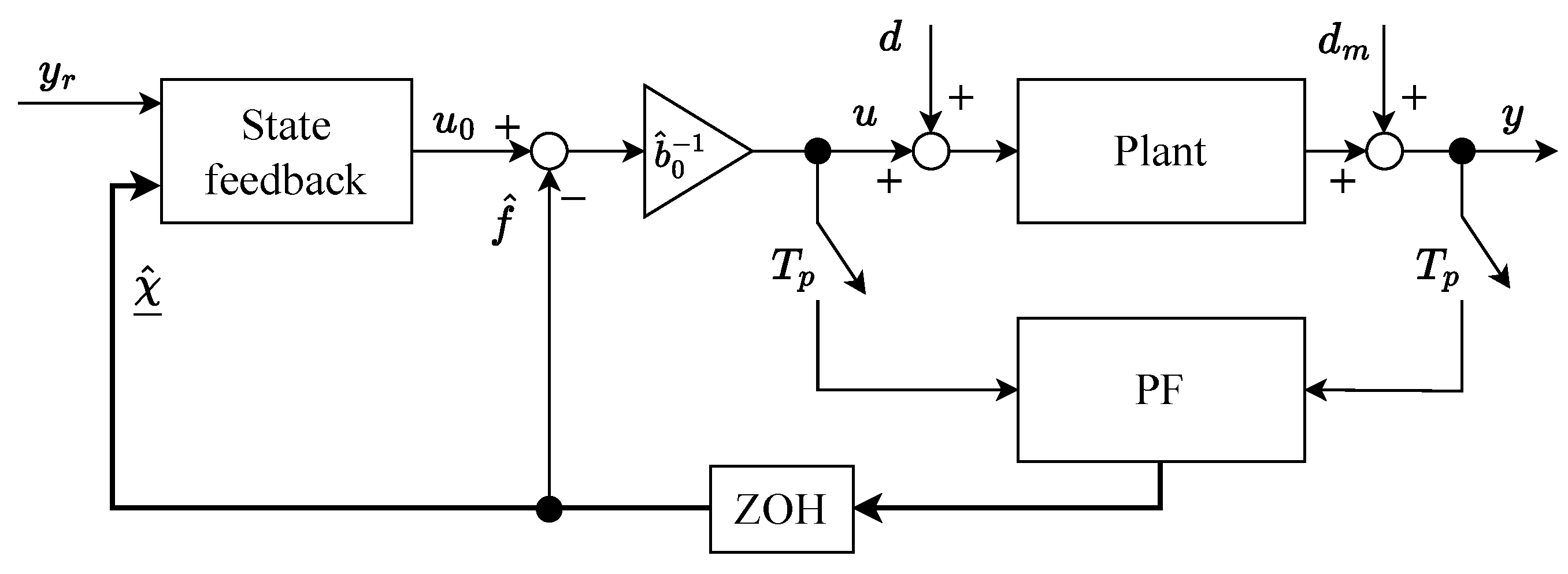
In the proposed approach, the conventional Extended State Observer is replaced by a particle filter estimating the augmented state vector for the ADRC. Instead of providing a single deterministic estimate, the PF represents the state and total disturbance by a set of weighted particles. The resulting control structure is shown in Figure 1.

For the particle-filter implementation, the continuous-time model introduced in Section 2 is sampled with period $T_s$. In the following, $\underline{x}\left(k\right)\equiv \underline{x}\left(k{T}_s\right)$, $y\left(k\right)\equiv y\left(k{T}_s\right)$, and $u\left(k\right)\equiv u\left(k{T}_s\right)$ denote the corresponding sampled signals, and $k\in \mathbb{N}$ denotes the discrete-time index. The discrete-time extended-state model (4) is written as

$$\left\{\begin{array}{cc}\hfill \underline{x}(k+1)& ={\mathbf{A}}_d\underline{x}\left(k\right)+{\underline{b}}_d\left[{\widehat{b}}_{0}u\left(k\right)+\psi \left(\underline{\chi }\left(k\right)\right)\right]+\underline{v}\left(k\right),\hfill \\ \hfill y\left(k\right)& ={\underline{c}}^{\mathrm{T}}\underline{x}\left(k\right)+d_m\left(k\right),\hfill \end{array}\right.$$

(17)

where $d_m\left(k\right)$ is the measurement noise. The discrete-time matrices with sample time $T_s$ are obtained as

$${\mathbf{A}}_d=e^{\mathbf{A}{T}_s},{\underline{b}}_d={\int }_0^{T_s}{e}^{\mathbf{A}\tau }\underline{b}d\tau ,{\underline{g}}_d={\int }_0^{T_s}{e}^{\mathbf{A}\tau }\underline{h}d\tau ,$$

(18)

$${\underline{g}}_d^{\mathrm{T}}=\left[\begin{array}{ccccccccc}{\displaystyle \frac{T_s^{n+1}}{(n+1)!}}& & {\displaystyle \frac{T_s^n}{n!}}& & \dots & & {\displaystyle \frac{T_s^2}{2!}}& & T_s\end{array}\right]\stackrel{n=2}{\underset{T_s=0.01\mathrm{s}}{=}}\left[\begin{array}{ccccc}1.67·{10}^{-7}& & 5.00·{10}^{-5}& & 1.00·{10}^{-2}\end{array}\right].$$

(19)

Remark 3

(Sampled-data model interpretation). It should be emphasized that (17) represents the sampled state-transition and measurement model employed by the particle filter, rather than the complete closed-loop dynamics. The structural controllability and observability properties underlying the ADRC design are discussed in Section 2. Note that only the output $y\left(k\right)$ is directly measured, whereas $\underline{x}\left(k\right)$ denotes the latent augmented state, including the physical states and total disturbance, reconstructed by the PF.

For the canonical integrator-chain structure considered here and any $T_s>0$, the exact zero-order hold (ZOH) discretization in (18) preserves the corresponding rank properties: the n-dimensional physical subsystem remains controllable and the complete augmented discrete-time model remains observable, whereas the additional total-disturbance state remains uncontrollable through the plant input. The stability of the resulting sampled-data closed-loop system is analyzed separately in Section 5.

Assuming that $\dot{f}$ is constant within each sampling interval, the process uncertainty is modeled as

$$\underline{v}\left(k\right)={\underline{g}}_d{w}_f\left(k\right),\mathbb{E}\left\{w_f\left(k\right)\right\}=0,{\mathbf{Q}}_d=cov\left\{\underline{v}\left(k\right)\right\}=q{\underline{g}}_d{\underline{g}}_d^{\mathrm{T}}.$$

(20)

The principal uncertainty of the augmented ADRC model is related to the unknown evolution of the continuous total disturbance. For sufficiently small sampling periods, the components of ${\underline{g}}_d$ preceding its last component are of higher order in $T_s$ and may be neglected. Therefore, the process uncertainty is approximated as acting directly on the total-disturbance state:

$$\mathbf{Q}=\mathrm{cov}\left(\underline{v}\right)=diag(0,\dots ,0,q),$$

(21)

whereas the measurement-noise variance is denoted by

$$r=var\left\{d_m\right\}.$$

(22)

The measurement noise may follow an arbitrary probability density function (PDF), including Gaussian, heavy-tailed, multimodal, or other distributions. Let

$$\underline{Y}\left(k\right)={[y\left(1\right),y\left(2\right),\dots ,y\left(k\right)]}^{\mathrm{T}}$$

denote the available measurement sequence. The Bayesian update of the extended state is expressed as

$$\stackrel{\mathrm{posterior}\mathrm{PDF}}{\overbrace{p_x\left(\underline{x}\left(k\right)|\underline{Y}\left(k\right)\right)}}={\displaystyle \frac{\stackrel{\mathrm{likelihood}}{\overbrace{p\left(y\left(k\right)|\underline{x}\left(k\right)\right)}}\stackrel{\mathrm{prior}\mathrm{PDF}}{\overbrace{p_x\left(\underline{x}\left(k\right)|\underline{Y}(k-1)\right)}}}{\underset{\mathrm{normalizing}\mathrm{constant}}{\underbrace{p\left(y\left(k\right)|\underline{Y}(k-1)\right)}}}},$$

(23)

where $p_x\left(\underline{x}\left(k\right)\right|\underline{Y}\left(k\right))$ is the posterior PDF, $p\left(y\left(k\right)\right|\underline{x}\left(k\right))$ is the likelihood, $p_x\left(\underline{x}\left(k\right)\right|\underline{Y}(k-1))$ is the prior PDF, and $p\left(y\left(k\right)\right|\underline{Y}(k-1))$ is the evidence. The evidence is given by

$$p\left(y\left(k\right)|\underline{Y}(k-1)\right)={\int }_{{\mathbb{R}}^{n+1}}\left(p\left(y\left(k\right)|\underline{x}\left(k\right)\right)p_x\left(\underline{x}\left(k\right)|\underline{Y}(k-1)\right)\right)d\underline{x}\left(k\right).$$

(24)

The posterior density is approximated by $N_p$ weighted particles:

$${\widehat{p}}_x\left(\underline{x}\left(k\right)\mid \underline{Y}\left(k\right)\right)={\displaystyle \sum _{i=1}^{N_p}}{w}^i\left(k\right)\delta \left(\underline{x}\left(k\right)-{\underline{x}}^i\left(k\right)\right),$$

(25)

where ${\underline{x}}^i\left(k\right)$ and $w^i\left(k\right)$ denote the state and normalized weight of the i-th particle, respectively. $\delta (·)$ is the Dirac delta function.

The bootstrap particle filter used in this study consists of the following steps:

1.

Initialization: Define the initial particle values, set $k=1$

$${\underline{x}}^i\left(0\right)\sim p\left(\underline{x}\left(0\right)\right),w^i\left(0\right)={\displaystyle \frac{1}{N_p}}.$$

2.

Prediction: Sample each particle from the conditional state-transition density using the previous particle and the known control input

$$\begin{array}{cc}\hfill {\underline{x}}^i\left(k\right)& \sim p\left(\underline{x}\left(k\right)\mid {\underline{x}}^i(k-1),u(k-1)\right),\hfill \end{array}$$

(26)

$$\begin{array}{cc}\hfill {\underline{x}}^i\left(k\right)& ={\mathbf{A}}_d{\underline{x}}^i(k-1)+{\underline{b}}_d\left[{\widehat{b}}_{0}u(k-1)+\psi \left({\underline{\chi }}^i(k-1)\right)\right]+{\widehat{\underline{v}}}^i(k-1),\hfill \end{array}$$

(27)

$$\begin{array}{cc}\hfill {\widehat{\underline{v}}}^i(k-1)& \sim p_{\underline{v}}\left(\underline{v}\right).\hfill \end{array}$$

(28)

3.

Weight update: Calculate particle weights using the measurement model

$$w_{*}^i\left(k\right)=w^i(k-1)p\left(y\left(k\right)\mid {\underline{x}}^i\left(k\right)\right).$$

(29)

4.

Normalization: Scale the weights so that their sum equals one

$$w^i\left(k\right)={\displaystyle \frac{w_{*}^i\left(k\right)}{{\sum }_{l=1}^{N_p}{w}_{*}^l\left(k\right)}}.$$

(30)

5.

State estimation: Obtain the estimated state

$$\underline{\widehat{x}}\left(k\right)={\displaystyle \sum _{i=1}^{N_p}}{w}^i\left(k\right){\underline{x}}^i\left(k\right).$$

(31)

6.

Resampling: the particles are resampled according to their weights using systematic resampling [36].

Remark 4

(PF tuning). The parameter r should reflect the variance of the measurement noise, whereas q determines how rapidly the estimated total disturbance may vary. Increasing q improves the estimator response to rapid disturbance changes but generally increases estimation variability. In contrast to the Kalman-filter-based tuning proposed in [12], where the ratio $q/r=\mathrm{const}$ was employed and combined with observer poles, the PF parameters q and r should be selected separately, as particle propagation and likelihood evaluation depend on their absolute values and on the assumed noise PDF.

3.2. Integration of Particle Filtering with ADRC

The particle filter provides a posterior distribution of the extended state, rather than only a single state estimate. In the conventional PF-ADRC implementation [34], this distribution is reduced to its weighted mean:

$$\underline{\widehat{x}}\left(k\right)={\displaystyle \sum _{i=1}^{N_p}}{w}^i\left(k\right){\underline{x}}^i\left(k\right).$$

(32)

The last component of $\underline{\widehat{x}}\left(k\right)$ represents the estimated total disturbance $\widehat{f}\left(k\right)$ in the discrete-time domain, whereas the remaining components form the estimated physical state vector $\underline{\widehat{\chi }}\left(k\right)$. Using the posterior mean, the conventional PF-based ADRC law is given by

$$u_{\mathrm{CE}}\left(k\right)={\displaystyle \frac{1}{{\widehat{b}}_0}}\left[u_0\left(k\right)-\psi \left(\underline{\widehat{\chi }}\left(k\right)\right)-\widehat{f}\left(k\right)\right],$$

(33)

where $u_0$ is defined as (11) for $t=k{T}_s$. This structure may be interpreted as a certainty-equivalent (CE) controller because the complete posterior distribution is replaced by a single expected value.

To retain the information contained in the particle distribution, a candidate ADRC action is calculated for every particle:

$$u^i\left(k\right)={\pi }_k\left({\underline{x}}^i\left(k\right)\right)={\displaystyle \frac{1}{{\widehat{b}}_0}}\left[u_0^i\left(k\right)-\psi \left({\underline{\chi }}^i\left(k\right)\right)-{\widehat{f}}^i\left(k\right)\right],$$

(34)

where

$$u_0^i\left(k\right)=k_1{y}_r\left(k\right)-{\underline{k}}^{\mathrm{T}}{\underline{\chi }}^i\left(k\right).$$

(35)

Consequently, the weighted set

$$\mathcal{U}\left(k\right)={\left\{u^i\left(k\right),w^i\left(k\right)\right\}}_{i=1}^{N_p}$$

(36)

represents an empirical posterior distribution of the control action induced by the state posterior $p_x(\underline{x}\left(k\right)\mid \underline{Y}\left(k\right))$. The corresponding empirical posterior distribution of the control action is

$${\widehat{p}}_u\left(u\mid \underline{Y}\left(k\right)\right)={\displaystyle \sum _{i=1}^{N_p}}{w}^i\left(k\right)\delta \left(u-u^i\left(k\right)\right).$$

(37)

The expected control action is equal to

$$\overline{u}\left(k\right)=\mathbb{E}\left[u\left(k\right)\mid \underline{Y}\left(k\right)\right]={\displaystyle \sum _{i=1}^{N_p}}{w}^i\left(k\right)u^i\left(k\right).$$

(38)

Remark 5.

For an affine ADRC control mapping, averaging the particle-wise control actions is exactly equivalent to evaluating the control law at the posterior-mean extended-state estimate. Therefore, (38) does not define a new control law by itself. Its purpose is to expose the empirical posterior distribution of the required control action, which is subsequently used by the proposed risk-aware selection mechanism. For a nonlinear mapping $\psi \left(\underline{·}\right)$, the mean particle-wise action and the action evaluated at the posterior-mean state generally differ.

The posterior probability that the particle-wise required control action (34) exceeds the actuator limits can be estimated as

$$P_{\mathrm{sat}}\left(k\right)={\displaystyle \sum _{i=1}^{N_p}}{w}^i\left(k\right)\mathbb{I}\left(\left|u^i\left(k\right)\right|>U_{max}\right),$$

(39)

where $U_{max}$ denotes the actuator limit and $\mathbb{I}(·)$ is the indicator function. Unlike the conventional point-estimate formulation, (39) allows the controller to distinguish between a well-defined moderate control action and a similar mean value resulting from a wide or multimodal posterior distribution.

The posterior-mean action may exceed the admissible actuator range. Therefore, its constrained counterpart is defined as

$$u_{\mathrm{PM}}\left(k\right)={proj}_{[-U_{max},U_{max}]}\overline{u}\left(k\right)=min\left\{U_{max},max\left\{-U_{max},\overline{u}\left(k\right)\right\}\right\}.$$

(40)

The signal $u_{\mathrm{PM}}\left(k\right)$ constitutes the constrained posterior-mean PF-ADRC action and is used as the baseline for evaluating the effect of the risk-aware mechanism.

3.3. Risk-Aware Control Action Selection

The posterior-mean controller minimizes the expected squared difference between the selected control signal and the particle-wise ADRC actions. It does not, however, explicitly account for less probable but unfavorable state and disturbance realizations. To include this information, a risk-aware control law is proposed. For a candidate control signal $u^c$, the loss associated with the i-th particle is defined as

$${\ell }^i(u^c,k)={\left(u^c-u^i\left(k\right)\right)}^2.$$

(41)

Its expected value is

$$J_{\mathrm{E}}(u^c,k)={\displaystyle \sum _{i=1}^{N_p}}{w}^i\left(k\right){\mathsf{\ell }}^i(u^c,k).$$

(42)

Minimization of $J_{\mathrm{E}}$ alone results in the posterior-mean action $\overline{u}\left(k\right)$.

To penalize the unfavorable tail of the loss distribution, the Conditional Value-at-Risk measure is introduced:

$$J_{\mathrm{CVaR}}(u^c,k)=\underset{\zeta }{min}\left[\zeta +{\displaystyle \frac{1}{1-\alpha }}{\displaystyle \sum _{i=1}^{N_p}}{w}^i\left(k\right)max\left({\mathsf{\ell }}^i(u^c,k)-\zeta ,0\right)\right],$$

(43)

where $\alpha \in (0,1)$ determines the considered upper part of the loss distribution. For example, $\alpha =0.9$ emphasizes approximately the worst $10\%$ of the weighted particle realizations. The proposed risk-aware PF-ADRC action is selected according to

$$u_{\mathrm{RA}}\left(k\right)=arg\underset{\left|u^c\right|\le U_{max}}{min}\left[(1-\lambda )J_{\mathrm{E}}(u^c,k)+\lambda J_{\mathrm{CVaR}}(u^c,k)+\gamma {\left(u^c-u_{\mathrm{RA}}(k-1)\right)}^2+\eta {\left({\displaystyle \frac{u^c}{U_{max}}}\right)}^2\right].$$

(44)

The parameter $\lambda \in [0,1]$ determines the contribution of the risk term. For $\lambda =0$, the tail-risk term is removed. If, additionally, $\gamma =\eta =0$, the solution reduces to the posterior-mean action projected onto the admissible control interval. Increasing $\lambda$ gives more importance to particle realizations associated with large control errors.

The term weighted by $\gamma \ge 0$ limits rapid changes of the control input (adding discrete-time memory), whereas the term weighted by $\eta \ge 0$ penalizes the control magnitude relative to the actuator range. The constraint in (44) ensures that the final control signal remains within the admissible range. The CVaR term penalizes large particle-wise compensation errors associated with unfavorable posterior realizations, whereas the hard input constraint and the control-magnitude penalty explicitly account for actuator limitations.

Example 1

(Multimodal control-action posterior). Consider a control-action posterior with approximately $80\%$ of the particle weight concentrated around $u^i=-2$ and the remaining $20\%$ around $u^i=8$. The posterior-mean action is then

$$\overline{u}=0.8(-2)+0.2\left(8\right)=0,$$

(45)

although almost no particle indicates this value. For $\alpha =0.8$, $\lambda =1$, and $\gamma =\eta =0$, the CVaR-based criterion selects $u_{\mathrm{RA}}=3$, which minimizes the largest particle-wise compensation errors. The constraint $|u_{\mathrm{RA}}|\le U_{max}$ additionally ensures actuator feasibility.

As the optimization problem is scalar for a single-input system, it can be solved efficiently at every sampling instant. Therefore, the proposed approach does not require a prediction horizon and should not be interpreted as a form of stochastic model predictive control. It constitutes an additional decision-making layer applied directly to the conventional ADRC law.

3.4. Tuning and Implementation Remarks

The tuning guideline for the ADRC parameters, PF settings, and risk-aware parameters is presented below.

• The controller bandwidth ${\omega }_c$ and the input-gain estimate ${\widehat{b}}_0$ should first be selected using the conventional ADRC design procedure.
• The measurement-noise model should then be determined from sensor data or selected according to the expected operating conditions. The variance r and the corresponding probability density function define the particle likelihood.
• The process parameter q determines the admissible variation of the total-disturbance state and should be increased when faster disturbance tracking is required.
• The number of particles $N_p$ should be selected as the smallest value that provides repeatable estimation results without violating the required sampling period. The influence of $N_p$ should therefore be evaluated jointly in terms of estimation quality and computation time.
• In the grid-based implementation used in this work, the admissible interval $[-U_{max},U_{max}]$ is discretized into $N_{\mathrm{grid}}$ uniformly spaced candidate control actions $u^c$.
• First, set $\lambda =\gamma =\eta =0$ and verify the operation of the posterior-mean PF-ADRC.
• Then, select $\gamma$ and $\eta$ to reduce excessive control variations and operation close to the actuator limits, respectively.
• Finally, gradually increase $\lambda$ until the desired compromise between the average tracking performance and the robustness to unfavorable posterior realizations is obtained. The parameter $\alpha$ should be selected according to the fraction of the unfavorable tail to be emphasized.

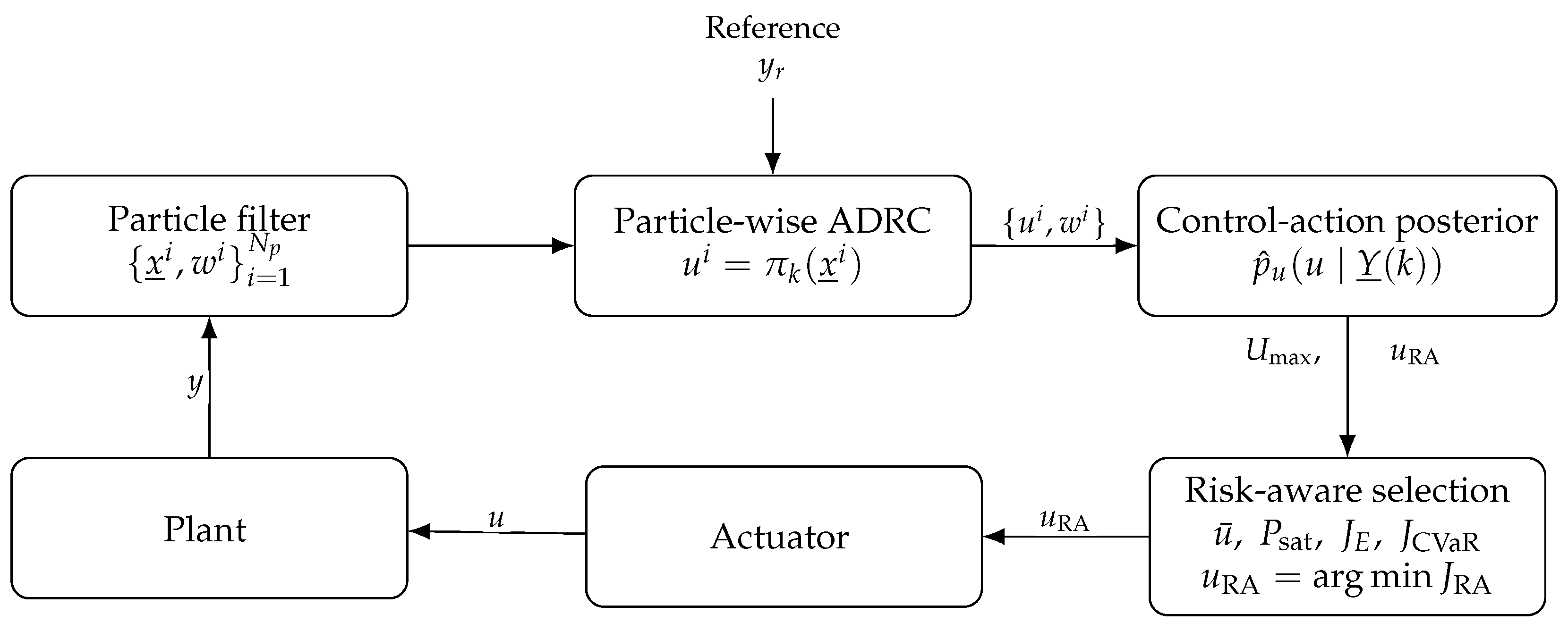
The action of the proposed method is shown in detail in Figure 2.

The practical interpretation of the risk-related parameters and the recommended direction of their tuning are summarized in

Table 1. Practical interpretation and tuning guidelines for the risk-aware parameters.

Parameter	Role	Qualitative Effect of Increasing the Parameter	Practical Tuning Guideline
$\lambda$	Relative weighting of the CVaR-based tail-risk term with respect to the expected-loss term.	Shifts the criterion from average particle-wise loss toward unfavorable tail realizations.	Start from $\lambda =0$ and gradually increase it while monitoring tracking performance, control effort, and sensitivity to unfavorable posterior realizations.
$\alpha$	CVaR confidence level; the corresponding upper-tail probability is approximately $1-\alpha$.	Focuses the risk term on a smaller and more extreme subset of the loss distribution.	Select according to the fraction of unfavorable realizations to be emphasized; e.g., $\alpha =0.8$ and $0.9$ correspond approximately to the worst $20\%$ and $10\%$ of weighted realizations, respectively.
$\gamma$	Penalty on the control-rate variation ${(u^c-u_{\mathrm{RA}}(k-1))}^2$.	Produces smoother control action but may reduce the ability to react rapidly to changes.	Increase when excessive sample-to-sample control variations are observed; avoid unnecessarily large values when fast disturbance compensation is required.
$\eta$	Penalty on the control magnitude normalized by the actuator range.	Discourages large control amplitudes and operation close to the actuator limits, but may weaken disturbance compensation if selected excessively.	Increase when excessive actuator utilization is observed; keep sufficiently small when substantial control authority is required.

. These recommendations constitute practical guidelines rather than an analytically optimal tuning rule. Adaptive or optimization-based selection of the risk parameters remains an important direction for future work.

Remark 6

(Particle number and computational cost). The number of particles should be selected empirically. As a heuristic guideline, an n-th-order ADRC plant may use $N_p\approx 4^{n+2}$ particles, increased up to ${10}^{n+2}$ when higher accuracy is required [37]. This gives approximately 64–${10}^3$ particles for $n=1$ and 256–${10}^4$ for $n=2$. The matrix–vector operations involved in the PF prediction scale as $\mathcal{O}\left(n^2\right)$ with the system order, and repeated for each of the $N_p$ particles, giving a computational cost approximately proportional to $N_p{n}^2$.

For the complete risk-aware formulation, the cost additionally depends on the number of candidate actions $N_{\mathrm{grid}}$. With the sorting-based CVaR evaluation, the overall computational cost is approximately proportional to $N_p{n}^2+N_{\mathrm{grid}}{N}_{p}log{N}_p$. Thus, while the system-order-dependent operations scale as $\mathcal{O}\left(n^2\right)$, both $N_p$ and $N_{\mathrm{grid}}$ directly increase the practical computational burden. The regularization terms add negligible overhead.

For real-time implementation, the particle prediction, likelihood calculation, and evaluation of the particle-wise control actions can be performed in parallel. The scalar problem in (44) may be solved using a short predefined grid, a one-dimensional convex optimization routine, or an equivalent numerical procedure. The mean and maximum execution times should be reported together with the selected sampling period.

4. Simulation Study

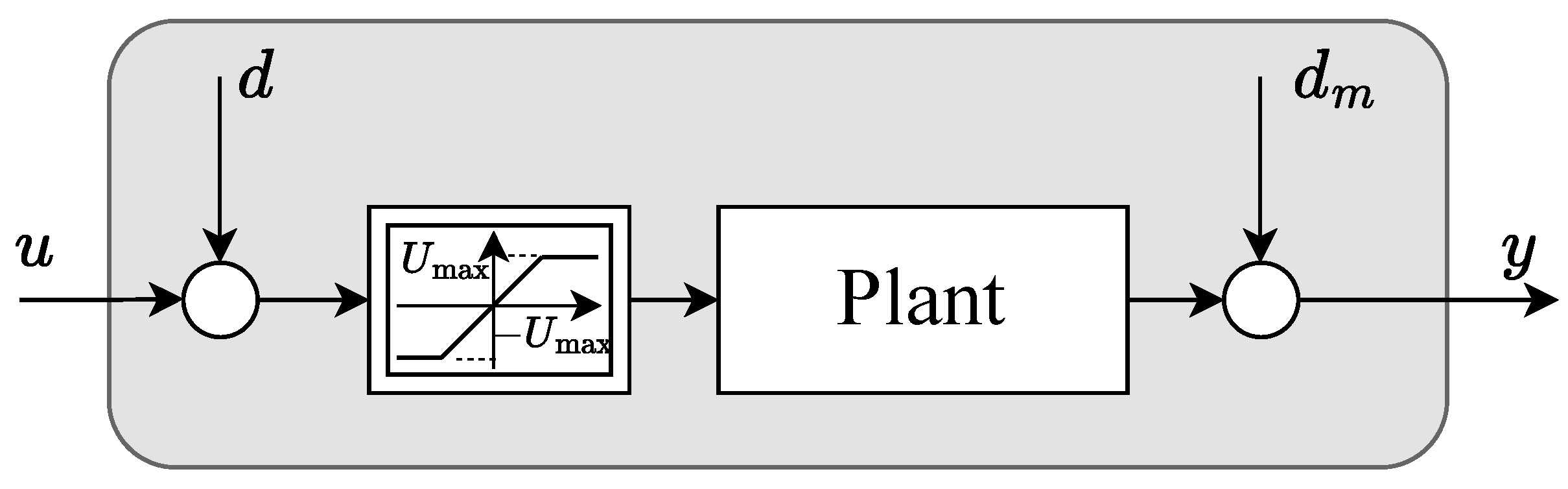
The following simulations constitute a concept-validation study intended to demonstrate how the extended-state posterior can be transferred to the control-action space under selected nonlinear, non-Gaussian, and constrained operating conditions. The general open-loop system considered in the study, disturbed by the external input d and measurement noise $d_m$, and also including control signal saturation, is presented in Figure 3.

The simulation study considers a reduced-order nonlinear model of a servo-driven rotary axis subjected to viscous damping, gravity-induced torque, and unknown load torque. Such dynamics are representative of rotary motion systems, including tilting axes used in multiaxis machine tools

$$J\ddot{\theta }+B\dot{\theta }+MgRsin\left(\theta \right)=K_{u}u+{\tau }_d,$$

(46)

where $\theta$ is the position on the rotary-axis, J is the equivalent moment of inertia, B denotes viscous damping, and $MgRsin\left(\theta \right)$ represents the gravity-induced torque resulting from the offset of the center of mass of the workpiece. The signal ${\tau }_d$ denotes an unknown load torque, which may include machining-induced disturbances transmitted to the rotary drive.

Let $y=\theta$ and define $d={\tau }_d/K_u$. Dividing the model by J gives

$$\ddot{y}=-a_1\dot{y}-a_{\psi }sin\left(y\right)+b_0\left(u+d\right),$$

(47)

where $a_1={\displaystyle \frac{B}{J}}$, $a_{\psi }={\displaystyle \frac{MgR}{J}}$, $b_0={\displaystyle \frac{K_u}{J}}$. The numerical parameters used throughout the simulation study are $a_1=5$, $a_{\psi }=6$, $b_0=40$, and, hence, the considered plant is

$$\ddot{y}+5\dot{y}+6sin\left(y\right)=40\left(u+d\right).$$

(48)

The plant parameters are kept unchanged in the following cases, whereas the measurement-noise distribution, disturbance profile, actuator constraints, and estimator configuration are varied. One can define the standard ADRC model components (1): $f(·)=-5\dot{y}+40d$ and $\psi (·)=-a_{\psi }sin\left(y\right)$ is assumed to be known.

Unless stated otherwise, the compared estimators were tuned to provide a practical compromise between disturbance tracking and measurement-noise sensitivity. The ESO and KF settings followed their conventional tuning principles, whereas the PF used an empirically selected process-noise variance and a measurement likelihood consistent with the assumed noise distribution. The parameter sets were kept unchanged across the considered scenarios.

Remark 7.

For linear models with Gaussian process and measurement noise, the Kalman filter provides the exact Bayesian mean and covariance, whereas the particle filter approximates the same posterior numerically [8]. This case was already investigated in the preliminary conference study [34]. Moreover, for small angular displacements, the nonlinear plant considered here is locally approximated by the same linear model. Therefore, the present study focuses on non-Gaussian measurement noise and risk-aware control-action selection.

Example 2 (Illustrative comparison under non-Gaussian measurement noise).

Consider the nonlinear plant defined in (48). The controller and estimator parameters are kept identical for all compared structures. A step disturbance $d\left(t\right)=5·\mathbf{1}\left(t-{\displaystyle \frac{t_{\mathrm{h}}}{2}}\right)$, where $t_{\mathrm{h}}$ is the time horizon, is introduced halfway through the simulation. The measurement noise follows the symmetric bimodal distribution

$$d_m\sim {\displaystyle \frac{1}{2}}\mathcal{N}\left(-m,{\sigma }_m^2\right)+{\displaystyle \frac{1}{2}}\mathcal{N}\left(m,{\sigma }_m^2\right),$$

(49)

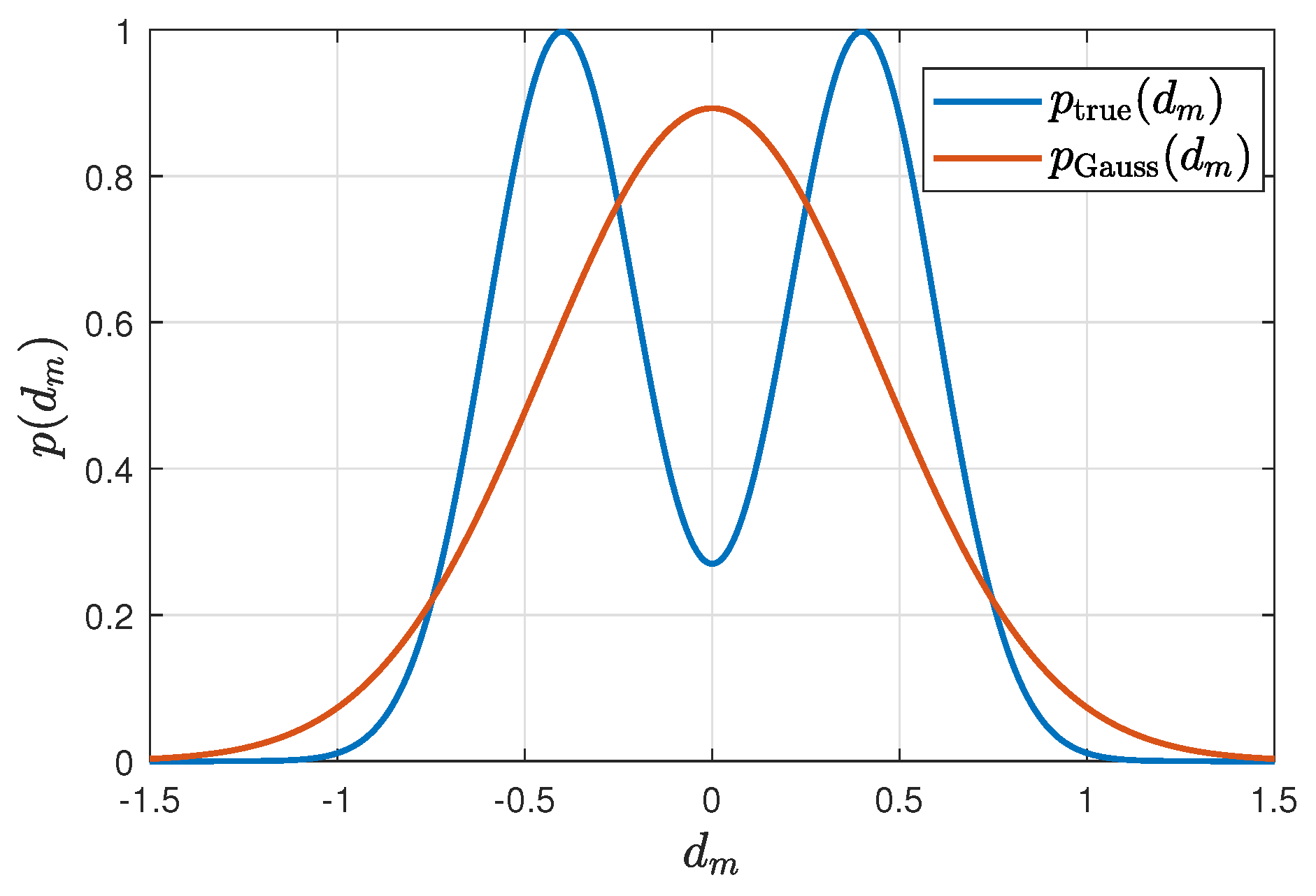
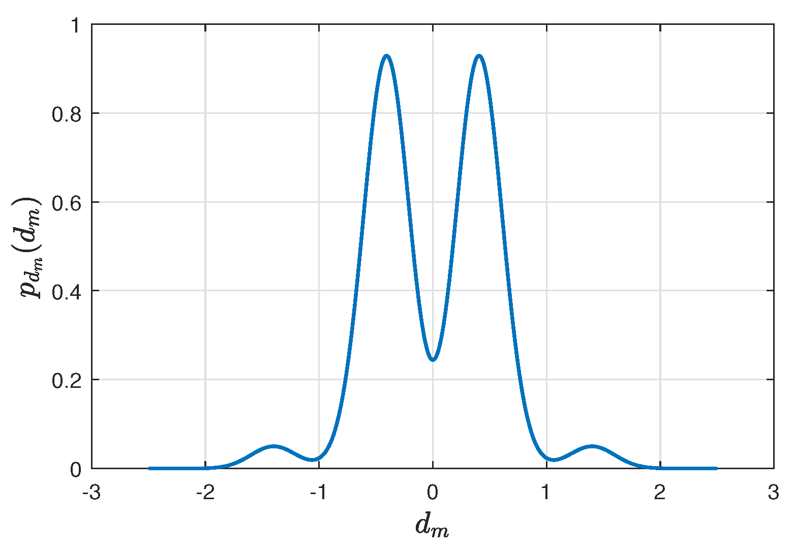
where the right-hand side denotes an equal-weight Gaussian mixture distribution rather than a sum of two Gaussian random variables, with parameters $m=0.4$ and ${\sigma }_m=0.2$. The PF evaluates the particle weights using the true likelihood (49), whereas the KF employs its Gaussian approximation with the same variance as $p\left(d_m\right)$: ${\sigma }_{\mathrm{Gauss}}^2=m^2+{\sigma }_m^2=0.2$, so the approximated distribution is defined as $p_{\mathrm{Gauss}}\sim \mathcal{N}(0,0.2)$ (see Figure 4).

The symmetric equal-weight bimodal distribution considered here is intended as a controlled representative model of multimodal measurement uncertainty rather than as an exact statistical model of a particular sensor. The numerical parameters and measurement-noise amplitudes are expressed in normalized coordinates and are selected to provide a challenging assessment of the proposed estimation and action-selection mechanisms.

The standard posterior-mean PF-ADRC structure is used, without the proposed risk-aware action-selection mechanism. Hence, the control input is calculated directly from the weighted posterior-mean state estimate. In the discrete-time implementation, sample time $T_s=0.01$ s was used. The controller and estimator parameters are selected as follows:

$$\left(\mathrm{ESO}\right):{\widehat{b}}_0=40,{\omega }_c=10,{\omega }_o=50,\left(\mathrm{KF}\right):q/r=8·{10}^4,$$

(50)

and for PF-based estimator:

$$\left(\mathrm{PF}\right):q=1.5·{10}^3,{\sigma }_m^2=0.2^2,N_p=800.$$

(51)

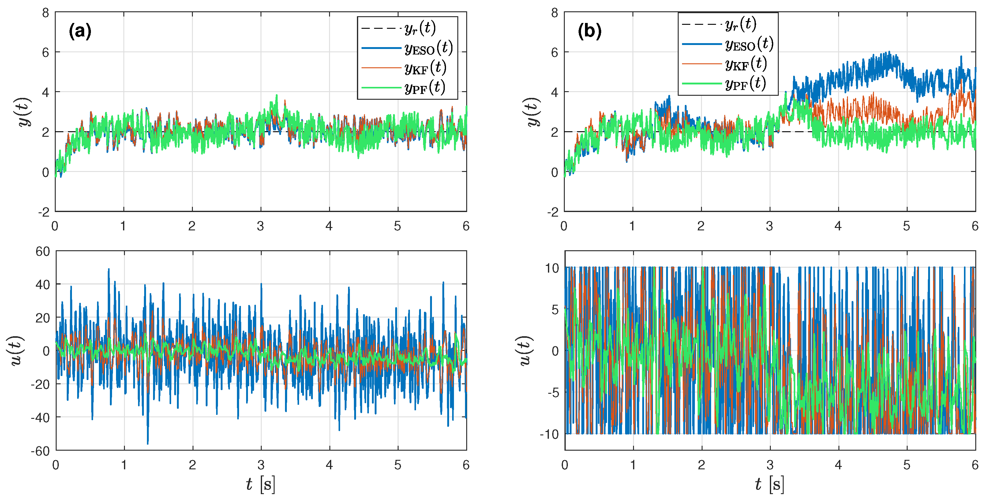
The results obtained without and with the actuator constraint $\left|u\right|\le U_{max}$ are shown in Figure 5.

Without the actuator constraint, all three ADRC structures stabilize the plant response and reject the applied disturbance. The main difference is observed in the control effort: the PF-based structure produces a less variable control signal and requires lower control energy because it directly incorporates the true non-Gaussian measurement likelihood.

When the actuator constraint is introduced, only the PF-based ADRC recovers the reference value after the disturbance d is applied. In the ESO- and KF-based structures, the estimated control demand is shifted toward the actuator boundary and exhibits larger variability. Consequently, the control signal repeatedly enters saturation and the available control authority becomes insufficient to compensate for the disturbance during the second half of the simulation. The example therefore provides an illustrative motivation for retaining the non-Gaussian posterior information in the subsequent risk-aware control-action selection.

Example 3 (Sensitivity to measurement-noise dispersion).

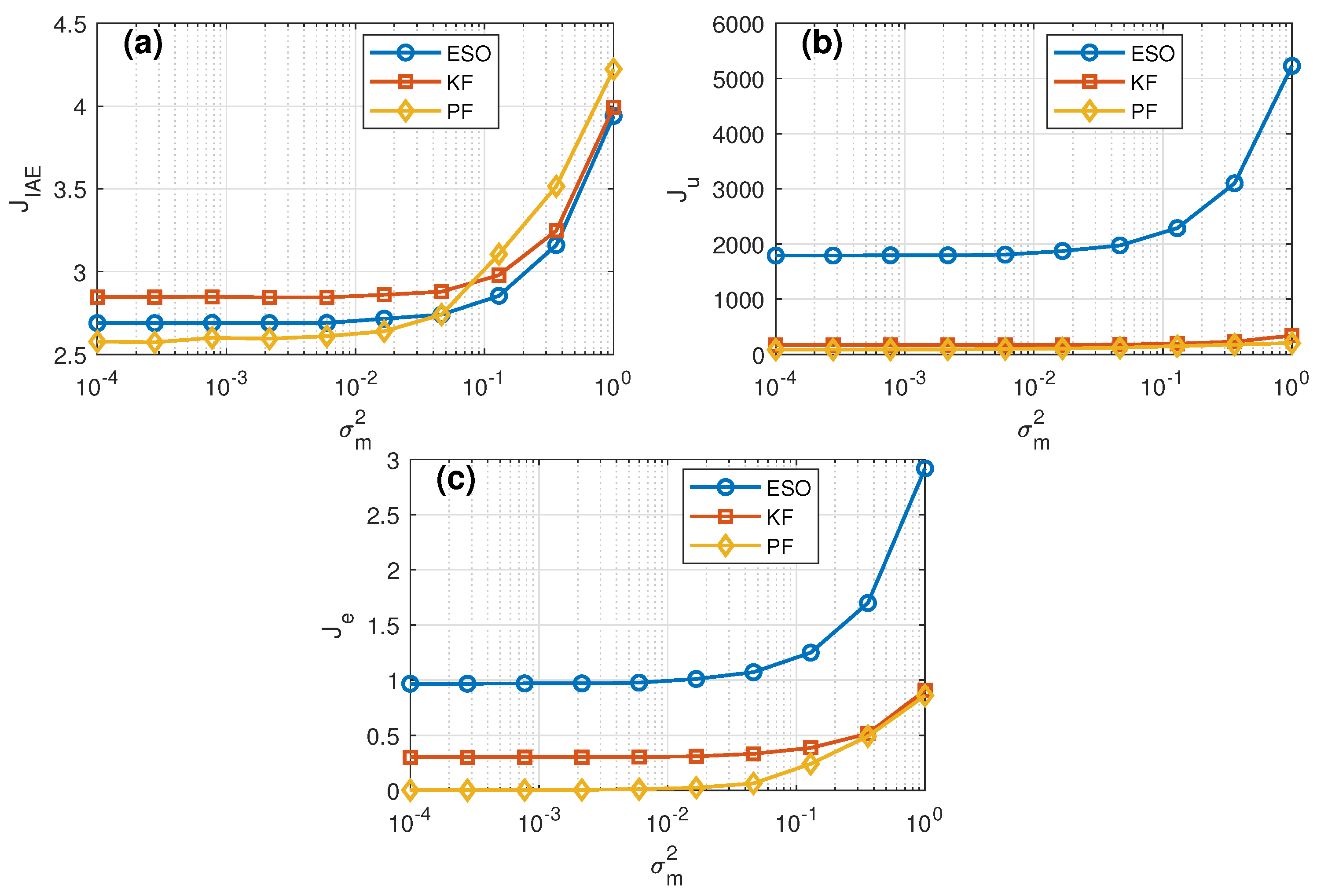
The nonlinear plant and the control conditions introduced in Example 2 are considered. The measurement noise follows the same symmetric bimodal distribution (49), whereas the variance of each Gaussian component is varied within the range

$${\sigma }_m^2\in \left\{{10}^{-4},\dots ,{10}^0\right\}.$$

(52)

The ESO and KF settings are the same as in Example 2. For the PF, the process-noise parameter is set to $q=1.5·{10}^3$, while the Gaussian-component variance used in the PF likelihood is adjusted according to ${\sigma }_m^2$. For each value of ${\sigma }_m^2$ (the original PDF is used), 100 Monte Carlo simulations are performed using different random-number-generator seeds.

Let $y^{\circ }$ denote the noise-free plant output (used here in the estimation quality evaluation, not available in practice), let $y=y^{\circ }+d_m$ denote the measured output, and $\widehat{y}={\underline{c}}^{\mathrm{T}}\underline{\widehat{x}}$ denote its estimate. The following performance indices are evaluated:

$$\begin{array}{cc}\hfill J_{\mathrm{IAE}}& ={\int }_0^{t_{\mathrm{h}}}\left|y_r-y\right|dt,\hfill \end{array}$$

(53)

$$\begin{array}{cc}\hfill J_u& ={\int }_0^{t_{\mathrm{h}}}{u}^{2}dt,\hfill \end{array}$$

(54)

$$\begin{array}{cc}\hfill J_{\mathrm{e}}& ={\int }_0^{t_{\mathrm{h}}}{\left(y^{\circ }-\widehat{y}\right)}^{2}dt.\hfill \end{array}$$

(55)

The values reported in Figure 6 are averaged over all Monte Carlo runs.

The results show that increasing the measurement noise variance degrades the performance of all compared structures. The PF provides the smallest estimation error and substantially lower control effort than the ESO, which is consistent with the ADRC law directly using the estimated states and total disturbance. For low and moderate noise levels, this also improves tracking quality; however, under the highest noise variance, the PF tracking error increases despite the favorable estimation and control-effort indices.

Example 4 (Risk-aware control under outlier-contaminated bimodal measurement noise).

The nonlinear plant defined in (48) is considered under bimodal measurement noise with sparse outliers. The posterior-mean PF-ADRC is compared with the proposed risk-aware action-selection variants. The measurement noise is modeled as a symmetric bimodal Gaussian mixture contaminated by sparse symmetric outliers (see Figure 7):

$$d_m\left(k\right)=\nu \left(k\right)+o\left(k\right),\nu \left(k\right)\sim {\displaystyle \frac{1}{2}}\mathcal{N}\left(-m,{\sigma }_m^2\right)+{\displaystyle \frac{1}{2}}\mathcal{N}\left(m,{\sigma }_m^2\right),$$

(56)

and $o\left(k\right)\in \{-A_{\mathrm{o}},0,A_{\mathrm{o}}\}$ with probabilities $p_{\mathrm{o}}/2$, $1-p_{\mathrm{o}}$, and $p_{\mathrm{o}}/2$, respectively. Thus, $\nu \left(k\right)$ follows an equal-weight symmetric Gaussian mixture rather than a linear combination of two Gaussian random variables. Although this mixture has zero mean, its variance is ${\sigma }_{d_m}^2=m^2+{\sigma }_m^2$ and its distribution is generally non-Gaussian. The parameters are set to $m=0.4$, ${\sigma }_m=0.2$, $p_{\mathrm{o}}=0.1$, and $A_{\mathrm{o}}=1$.

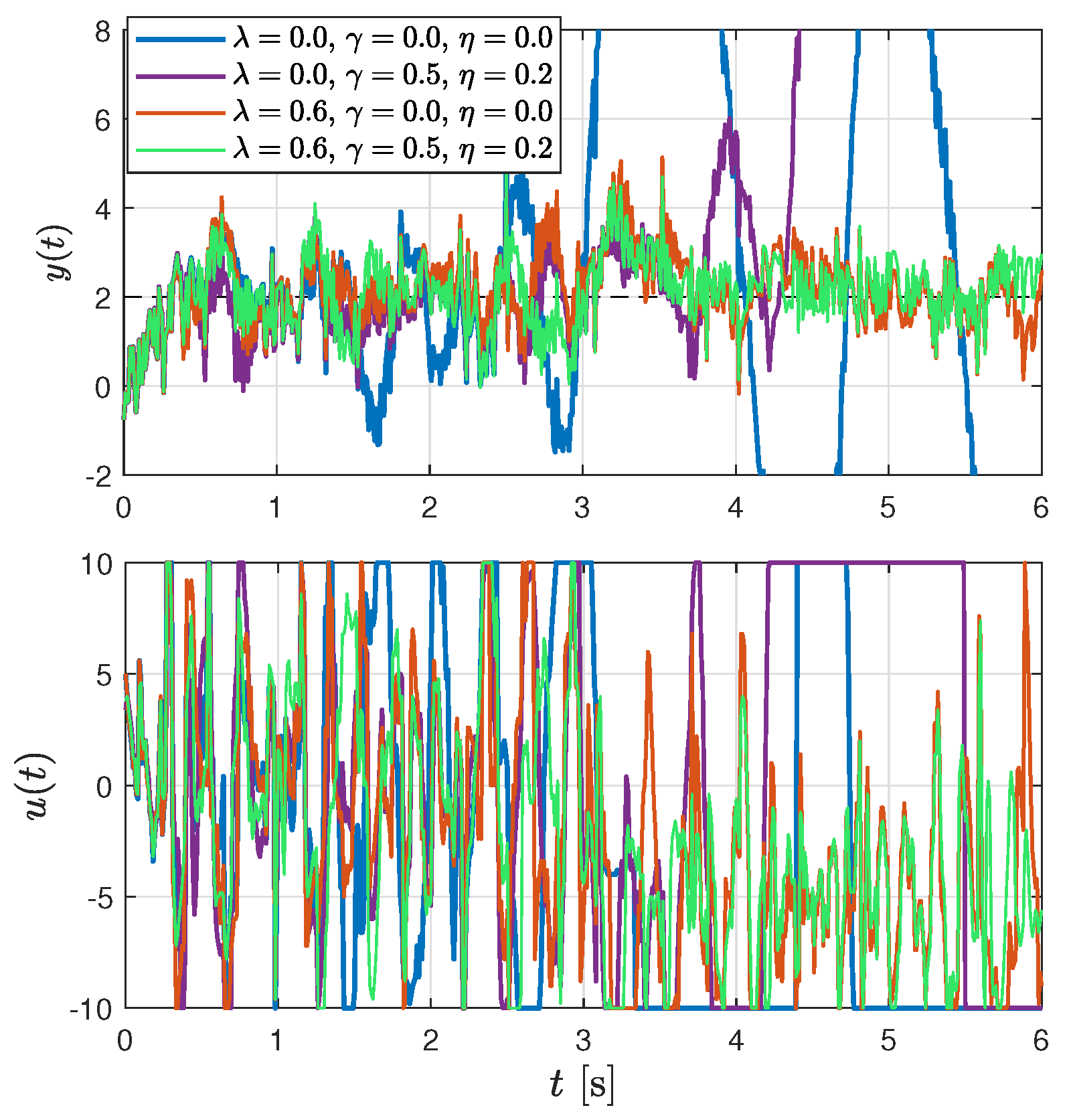
In the PF, the sparse outliers were not included in the assumed likelihood. Therefore, the example additionally evaluates robustness to measurement-model mismatch. To separate the effects of tail-risk penalization and control regularization, the simulations were carried out in four PF-based ADRC variants:

• (a) Posterior-mean control without risk-aware or regularization terms: $\lambda =\gamma =\eta =0$;
• (b) Posterior-mean control with control-rate and control-magnitude regularization: $\lambda =0$, $\gamma =0.5$, and $\eta =0.2$;
• (c) Risk-aware control with the CVaR contribution and without regularization terms: $\lambda =0.6$ and $\gamma =\eta =0$;
• (d) The complete risk-aware formulation combining the CVaR term with both regularization terms: $\lambda =0.6$, $\gamma =0.5$, and $\eta =0.2$.

For each case, $\alpha =0.8$ was assumed. For the grid-based implementation of the risk-aware action selection, $N_{\mathrm{grid}}=101$ uniformly spaced candidate control actions were considered over the interval $[-U_{max},U_{max}]$. The simulation results are shown in Figure 8, and

Table 2. Performance indices obtained for the considered action-selection variants. The symbols ✓ and × denote successful and failed runs, respectively.

Variant	${\mathit{J}}_{\mathbf{IAE}}$	${\mathit{J}}_{\mathit{u}}$	Success
(a)	31.0828	400.6630	×
(b)	141.3765	338.0886	×
(c)	4.1227	208.5880	✓
(d)	4.0984	187.9318	✓

presents the performance indices. The results show that the CVaR-based variants maintain satisfactory closed-loop operation, whereas the posterior-mean PF and the regularization-only variant lose tracking performance. This indicates that, for the considered noise realization, accounting for the unfavorable tail of the control-action distribution is essential.

The presented results support the feasibility of the proposed posterior-based action-selection concept. For the considered severe noise realization, the CVaR-based variants maintain satisfactory closed-loop operation, whereas the posterior-mean and regularization-only variants lose tracking performance. This single-run result illustrates the potential role of posterior tail information.

Example 5 (Monte Carlo assessment of risk-aware action selection).

To evaluate the repeatability of the results obtained in Example 4, a Monte Carlo study was performed for the same nonlinear plant, measurement-noise model, actuator constraint, and four action-selection variants. A total of $N_{\mathrm{MC}}=100$ simulations were conducted using different random-number-generator seeds. Within each Monte Carlo run, the same measurement-noise realization and the same initial particle set were applied to all variants to ensure a paired comparison.

The Monte Carlo results, shown in

Table 3. Monte Carlo performance of the considered action-selection variants.

Variant	$\mathbf{Median}\mathbf{\left(}{\mathit{J}}_{\mathbf{IAE}}\mathbf{\right)}$	${\mathit{Q}}_{95}\mathbf{\left(}{\mathit{J}}_{\mathbf{IAE}}\mathbf{\right)}$	$\mathbf{Median}\mathbf{\left(}{\mathit{J}}_{\mathit{u}}\mathbf{\right)}$	${\mathit{P}}_{\mathbf{succ}}$
(a)	12.0813	399.4017	242.2018	44%
(b)	5.1118	333.9042	231.1726	52%
(c)	4.5681	347.4316	223.8619	53%
(d)	5.1438	369.5863	218.4707	54%

, are summarized using the median values of $J_{\mathrm{IAE}}$ and $J_u$, while $Q_{95}\left(J_{\mathrm{IAE}}\right)$ denotes the 95th percentile of the $J_{\mathrm{IAE}}$ values and characterizes unfavorable tracking-error realizations. The empirical success rate is defined as

$$P_{\mathrm{succ}}={\displaystyle \frac{N_{\mathrm{succ}}}{N_{\mathrm{MC}}}}={\displaystyle \frac{1}{N_{\mathrm{MC}}}}{\displaystyle \sum _{j=1}^{N_{\mathrm{MC}}}}\mathbb{I}\left({\displaystyle \frac{1}{N_e}}{\displaystyle \sum _{k=N-N_e+1}^N}\left|2-y_j\left(k\right)\right|<2\right),$$

(57)

where N is the total number of samples, and $N_e=1/T_s$ is the sample number in the considered time horizon (the last one second of simulation here).

The Monte Carlo results indicate that the proposed posterior-based action-selection modifications generally improve the closed-loop performance compared with the posterior-mean PF baseline. The modified variants provide lower median tracking error, reduced control effort, and a higher empirical success rate, although no single configuration is uniformly superior with respect to all considered indices. The results should therefore be interpreted primarily as an initial validation of the proposed concept and as a characterization of its performance trade-offs rather than as evidence of universally improved or optimal risk-aware tuning.

Example 6 (Computational-time analysis).

To quantitatively assess the computational overhead of the considered approaches, the execution time of the controller-algorithm function was measured, excluding the plant simulation, Simulink solver, visualization, and other simulation-related overhead. The timing analysis was performed for the same second-order plant and nominal PF-ADRC settings used in the preceding simulation examples, unless stated otherwise. All measurements were performed on a desktop computer equipped with an Intel Core i5-7400 @ 3.00 GHz processor and 24 GB of DDR4 @ 2133 MHz RAM, running Windows 10 Pro operating system, version 22H2 (build 19045.6466), using MATLAB/Simulink R2023a. For each controller variant, 1000 function calls were evaluated under the nominal settings used in the preceding simulations. The mean execution time, 95th percentile ($Q_{95}$), maximum observed execution time, and the mean execution time relative to the sampling period $T_s=10$ ms are summarized in

Table 4. Execution-time statistics for the ESO-, KF-, and PF-based ADRC variants under the nominal simulation settings.

Variant	Mean [ms]	${\mathit{Q}}_{95}$ [ms]	Max [ms]	Mean/${\mathit{T}}_{\mathit{s}}$ [%]
ESO	0.0026	0.0021	0.3304	0.03
KF	0.0084	0.0088	0.3434	0.08
PF (a)	0.7481	0.8341	2.1979	7.48
PF (b)	0.8218	0.8472	2.0983	8.22
PF (c)	3.8791	4.1613	7.8307	38.79
PF (d)	3.9454	4.2907	6.6057	39.45

.

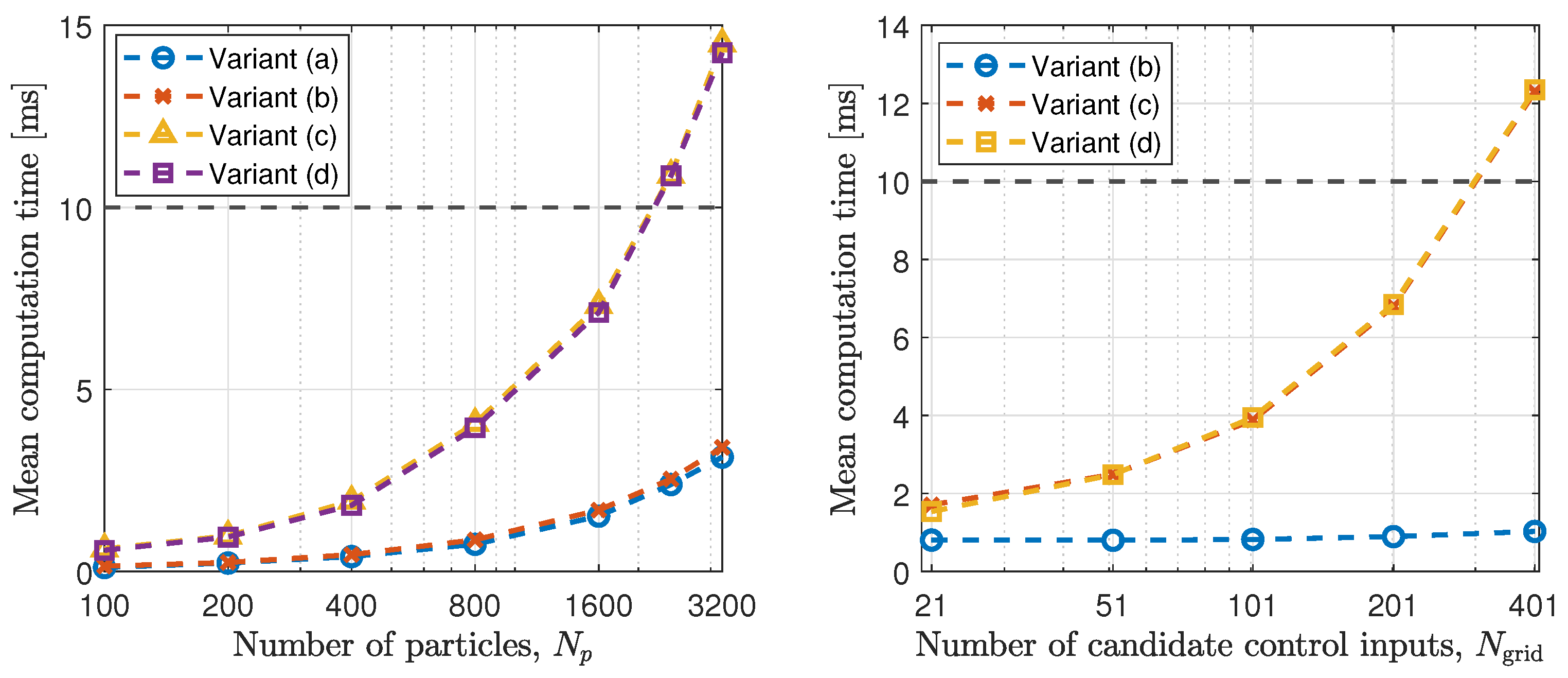
To additionally assess computational scalability, the measurements were repeated for varying numbers of particles $N_p$ and candidate control actions $N_{\mathrm{grid}}$. When varying $N_p$, $N_{\mathrm{grid}}=101$ was kept at its nominal value, whereas $N_p=800$ was fixed at its nominal value when varying $N_{\mathrm{grid}}$. The results are shown in Figure 9.

The execution times of the ESO and KF are negligible relative to the sampling period. The non-CVaR PF variants (a) and (b) require less than $10\%$ of $T_s$ on average, whereas the CVaR-based variants (c) and (d) require approximately $39\%$ of $T_s$. The computation time increases with $N_p$ for all PF-based variants, whereas increasing $N_{\mathrm{grid}}$ primarily affects the CVaR-based variants. For the nominal value $N_{\mathrm{grid}}=101$, the mean execution time of variant (d) reaches the sampling-period threshold at approximately $N_p=2400$. Variants (a) and (b), as well as (c) and (d), exhibit nearly identical execution times because the additional regularization terms introduce only negligible computational overhead compared with the dominant PF and CVaR computations. Overall, the results indicate computational feasibility for the nominal settings, while more efficient implementations may further reduce the execution time.

Example 7 (Validation on a higher-order nonlinear system: reaction-wheel pendulum).

To complement the preceding studies based on the second-order nonlinear plant and to provide a preliminary assessment of the applicability of the proposed framework to a more complex plant, an additional simulation study was performed for the third-order nonlinear reaction-wheel pendulum (RWP) described in detail in [38]. The RWP is a higher-order, nonlinear, and underactuated system whose input–output dynamics can be expressed as

$$\ddot{\phi }=-{\alpha }_i{\int }_0^{t}sin\left(\phi \left(\tau \right)\right)d\tau -{\alpha }_0\phi -{\alpha }_1\dot{\phi }-{\alpha }_{s}sin\left(\phi \right)-b_{0}u,$$

(58)

where the coefficients ${\alpha }_i=5.6973$, ${\alpha }_0=0.0330$, ${\alpha }_1=0.8088$, and ${\alpha }_s=4.3619$ result from the physical parameters of the original nonlinear RWP model, and $b_0=0.3388$ represents the corresponding input gain. The ADRC-compatible formulation proposed in [38] was used for controller and estimator design, while the bimodal measurement noise considered in the present study was additionally introduced.

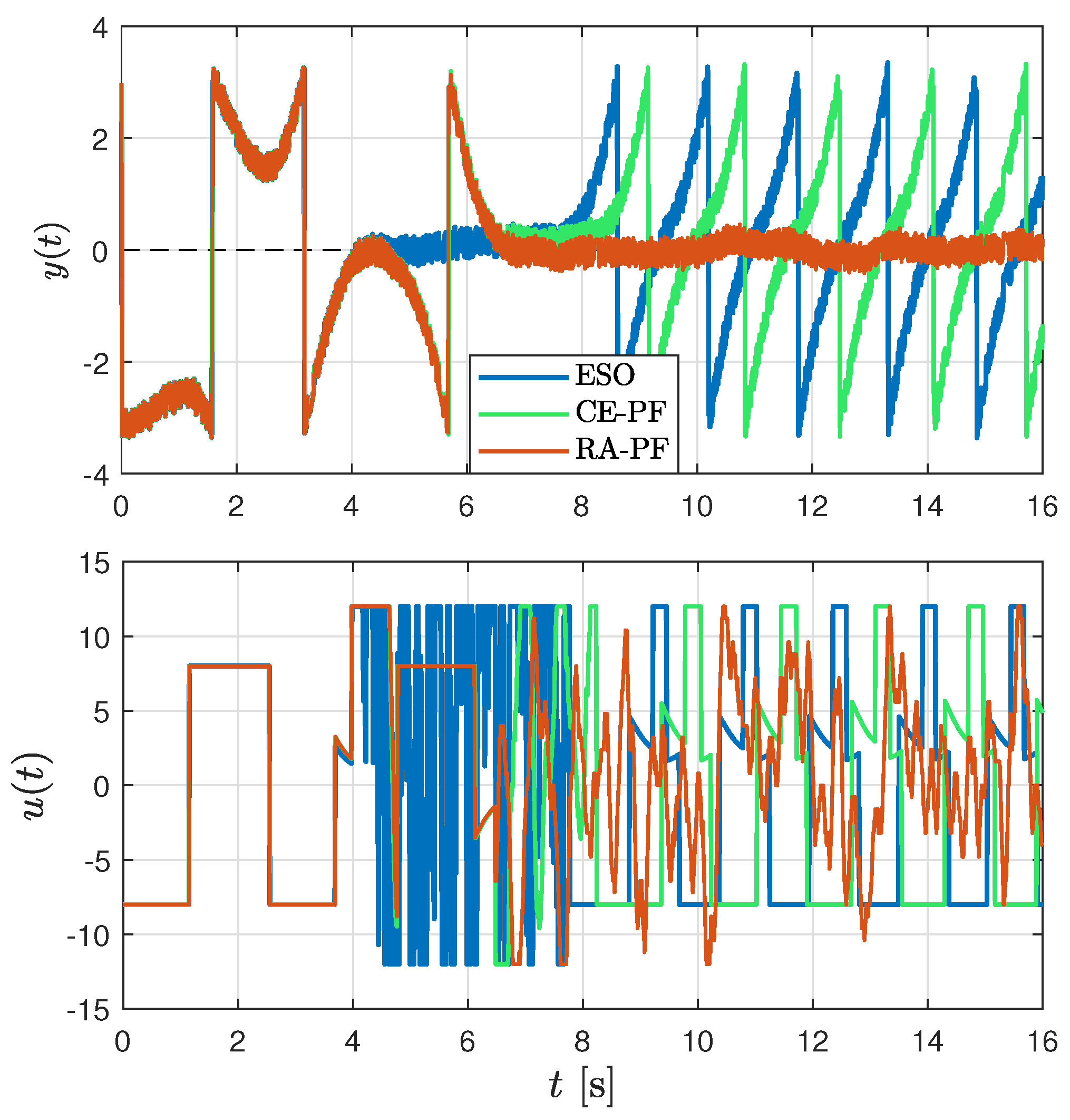
The measurement noise followed the symmetric bimodal Gaussian mixture (49) with $m=0.2$ and ${\sigma }_m^2=0.{04}^2$. The parameters were ${\omega }_c=3$, ${\omega }_o=10$, and, for the PF, $N_p=4000$, $N_{\mathrm{grid}}=31$. The PF employed a bimodal measurement likelihood of the same form, with empirically selected noise-variance parameters $q=200$ and $r=10$ for the process and measurement models, respectively. The risk-aware variant additionally used $\lambda =0.05$, $\alpha =0.9$, $\gamma =0.6$, and $\eta =0.09$. The actuator was constrained to $\left|u\right|\le 12$ V. The pendulum position was normalized with respect to the unstable upper equilibrium, corresponding to the reference value $y_r=0$, with the normalized angular position restricted to the range $[-\pi ,\pi ]$. Outside the stabilization region $\left|y\right|<0.3$ rad, the same swing-up controller was employed for all variants. The sampling period of the RWP was $T_s=0.01$ s. The RWP study was performed offline and is intended as a preliminary validation of the proposed approach rather than as a real-time implementation study. The simulation results can be found in Figure 10.

The preliminary results show that the ESO-based ADRC exhibits high control variability; increasing ${\omega }_o$ further amplifies the measurement noise, whereas lower values result in insufficiently fast estimation. The CE-PF improves the behavior but remains sensitive to the considered uncertainty. The proposed risk-aware action selection mitigates part of these limitations and maintains the pendulum near the upper equilibrium under the imposed actuator constraint in the considered simulation scenario. A more systematic investigation of the RWP case is left for future work.

5. Stability and Robustness Interpretation

This section provides a compact stability interpretation of the ESO- and PF-based ADRC structures. The deterministic ESO result is recalled as a reference for the probabilistic analysis of the proposed PF-ADRC. To remain consistent with the estimator and control laws, the known model term is assumed to depend on the physical state, i.e., $\psi =\psi \left(\underline{\chi }\right)$. Known input-dependent terms may instead be incorporated into the total disturbance f. Detailed derivations are provided in Appendix A.

5.1. Closed-Loop Tracking-Error Dynamics

Consider the plant (1): $y^{\left(n\right)}=\psi \left(\underline{\chi }\right)+{\widehat{b}}_{0}u+f$, where $\underline{\chi }={[y\dot{y}\dots y^{(n-1)}]}^{\top }$ and ${\widehat{b}}_0\ne 0$. The basic ADRC structure is obtained for $\psi \left(\underline{\chi }\right)=0$. A known nonlinear term, which is Lipschitz, may be included, for example, $\psi \left(\underline{\chi }\right)=a_{\psi }sin\left({\chi }_1\right)$.

Let

$$\underline{e}={\underline{\chi }}_r-\underline{\chi },\underline{\tilde{x}}=\underline{x}-\underline{\widehat{x}}={\left[\begin{array}{cc}{\underline{\tilde{\chi }}}^{\top }& \tilde{f}\end{array}\right]}^{\top },$$

(59)

where $\underline{\tilde{\chi }}=\underline{\chi }-\underline{\widehat{\chi }}$ and $\tilde{f}=f-\widehat{f}$. The certainty-equivalent ADRC action for the general trajectory tracking case is defined as

$$u_{\mathrm{CE}}={\displaystyle \frac{1}{{\widehat{b}}_0}}\left[y_r^{\left(n\right)}+{\underline{k}}^{\top }\left({\underline{\chi }}_r-\underline{\widehat{\chi }}\right)-\psi \left(\underline{\widehat{\chi }}\right)-\widehat{f}\right].$$

(60)

For the constrained and risk-aware structure, the deviation from the certainty-equivalent action is defined as

$$\Delta u_{\mathrm{A}}=u_{\mathrm{A}}-u_{\mathrm{CE}},$$

(61)

where $u_{\mathrm{A}}$ denotes the control action actually applied to the plant. Although the applied action $u_A\left(k\right)$ is constrained by the actuator limits, boundedness of $\Delta u_A$ does not follow from this constraint alone, because the unconstrained certainty-equivalent action $u_{\mathrm{CE}}\left(k\right)$ may be unbounded. Therefore, boundedness of $\Delta u_A\left(k\right)$ is introduced explicitly in the subsequent analysis. Substitution of (60) and (61) into (1) gives

$$e^{\left(n\right)}=-{\underline{k}}^{\top }\underline{e}-\xi ,$$

(62)

where

$$\xi ={\underline{k}}^{\top }\underline{\tilde{\chi }}+\psi \left(\underline{\chi }\right)-\psi \left(\underline{\widehat{\chi }}\right)+\tilde{f}+{\widehat{b}}_0\Delta u_{\mathrm{A}}.$$

(63)

Assumption 2 (Regularity of the embedded model).

The function $\psi (·)$ is Lipschitz continuous in the considered operating set:

$$\left|\psi \left({\underline{\chi }}_1\right)-\psi \left({\underline{\chi }}_2\right)\right|\le L_{\psi }∥{\underline{\chi }}_1-{\underline{\chi }}_2∥.$$

(64)

Lemma 1 (Tracking-error robustness).

Suppose that the feedback gains $\underline{k}$ define a Hurwitz closed-loop matrix. Under Assumption 2, there exist positive constants $c_1$, $c_2$, and $c_3$ such that

$${\dot{V}}_e\le -c_1\parallel \underline{e}{\parallel }^2+c_2\parallel \underline{\tilde{x}}{\parallel }^2+c_3{|\Delta u_{\mathrm{A}}|}^2,$$

(65)

where $V_e$ is a quadratic Lyapunov function. Consequently, the nominal tracking-error dynamics are input-to-state stable (ISS) with respect to the extended-state estimation error and the control action modification $\Delta u_A$. This inequality alone does not guarantee boundedness of the tracking error unless both input terms are bounded.

Proof. 

See Appendix A.1. □

5.2. Deterministic ESO-Based Estimation

Let the measured output be $y=y^o+d_m$. Assuming that the ESO uses $\psi \left(\underline{\widehat{\chi }}\right)$ and the same applied control signal as the plant, its estimation-error dynamics are

$$\dot{\underline{\tilde{x}}}={\mathbf{H}}_o\underline{\tilde{x}}+\underline{b}\left[\psi \left(\underline{\chi }\right)-\psi \left(\underline{\widehat{\chi }}\right)\right]+\underline{h}\dot{f}-\underline{l}{d}_m,$$

(66)

where ${\mathbf{H}}_o=\mathbf{A}-\underline{l}{\underline{c}}^{\top }$ is Hurwitz.

Assumption 3 (Bounded ESO inputs).

The signals affecting the ESO error satisfy

$$\left|\dot{f}\right|\le {\overline{d}}_f,\left|d_m\right|\le {\overline{d}}_m.$$

(67)

Proposition 1 (ESO error boundedness).

Let Assumptions 2 and 3 hold. If the observer dynamics are sufficiently dominant with respect to the Lipschitz term, then there exist positive constants $c_o$, $c_f$, and $c_m$ such that

$${\dot{V}}_o\le -c_o{\parallel \underline{\tilde{x}}\parallel }^2+c_f{\overline{d}}_f^2+c_m{\overline{d}}_m^2.$$

(68)

Consequently, the ESO estimation error is uniformly ultimately bounded. Together with Lemma 1, this also implies ultimate boundedness of the tracking error for the conventional ESO-based ADRC, for which $\Delta u_{\mathrm{A}}=0$.

Proof. 

See Appendix A.1. □

The deterministic result concerns bounded measurement perturbations, which represent physical sensors with finite measurement ranges. The stochastic measurement models used in the PF analysis are considered separately below.

5.3. Mean-Square Boundedness of PF-ADRC

Let

$$\underline{\widehat{x}}\left(k\right)={\displaystyle \sum _{i=1}^{N_p}}w{\left(k\right)}^i{\underline{x}}^i\left(k\right)$$

(69)

denote the weighted posterior mean evaluated before resampling, and let

$$\underline{\mu }\left(k\right)=\mathbb{E}\left[\underline{x}\left(k\right)\mid \underline{Y}\left(k\right)\right]$$

(70)

be the exact Bayesian posterior mean.

Assumption 4 (Uniform PF estimation bounds).

There exist constants ${\overline{\sigma }}_B^2>0$ and $C_{\mathrm{PF}}>0$, independent of k and $N_p$, such that

$$\underset{k\ge 0}{sup}\mathbb{E}\left[\parallel \underline{x}\left(k\right)-\underline{\mu }{\left(k\right)\parallel }^2\right]\le {\overline{\sigma }}_B^2,$$

(71)

and

$$\underset{k\ge 0}{sup}\mathbb{E}\left[\parallel \underline{\mu }\left(k\right)-\underline{\widehat{x}}{\left(k\right)\parallel }^2\right]\le {\displaystyle \frac{C_{\mathrm{PF}}}{N_p}}.$$

(72)

The second inequality represents the standard finite-particle approximation rate under suitable transition-model, likelihood, resampling, and bounded-moment conditions. It is treated here as an estimator property rather than independently proved for the particular bootstrap PF.

Lemma 2

(PF estimation-error bound). Under Assumption 4,

$$\underset{k\ge 0}{sup}\mathbb{E}\left[\parallel \underline{\tilde{x}}{\left(k\right)\parallel }^2\right]\le 2{\overline{\sigma }}_B^2+{\displaystyle \frac{2C_{\mathrm{PF}}}{N_p}}.$$

(73)

Proof. 

See Appendix A.2. □

Assumption 5 (Bounded risk-aware control modification).

For the considered closed-loop operating region, there exists a constant ${\overline{\sigma }}_u^2<\infty$, independent of k, such that

$$\underset{k\ge 0}{sup}\mathbb{E}\left\{{\left|\Delta u_{\mathrm{A}}\left(k\right)\right|}^2\right\}\le {\overline{\sigma }}_u^2.$$

(74)

This condition is assumed explicitly and is not implied solely by the actuator constraint, as $u_{\mathrm{CE}}$ is not itself constrained. Nevertheless, a simple sufficient condition can be given. As $|u_{\mathrm{A}}\left(k\right)|\le U_{max}$ for the constrained risk-aware implementation,

$$|\Delta u_{\mathrm{A}}{\left(k\right)|}^2\le 2U_{max}^2+2{\left|u_{\mathrm{CE}}\left(k\right)\right|}^2.$$

(75)

Hence, if

$$\underset{k\ge 0}{sup}\mathbb{E}\left\{|u_{\mathrm{CE}}{\left(k\right)|}^2\right\}<\infty ,$$

(76)

then the assumption is satisfied with a finite ${\overline{\sigma }}_u^2$. This condition may be established for a prescribed bounded operating region or verified numerically during closed-loop validation. Thus, Assumption 5 should be interpreted as a conditional requirement on the operating regime rather than as a consequence of the actuator constraint itself.

Theorem 1 (Conditional mean-square boundedness of the PF-ADRC tracking error).

Suppose that Assumptions 2, 4 and 5 hold, and that the nominal sampled closed-loop dynamics are Schur stable. Then there exists a constant $C_e>0$ such that

$$\underset{k\to \infty }{lim\; sup}\mathbb{E}\left[\parallel \underline{e}{\left(k\right)\parallel }^2\right]\le C_e\left({\overline{\sigma }}_B^2+{\displaystyle \frac{C_{\mathrm{PF}}}{N_p}}+{\overline{\sigma }}_u^2\right).$$

(77)

Proof. 

See Appendix A.2. □

For the unconstrained mean-state certainty-equivalent PF-ADRC, $u_{\mathrm{A}}\left(k\right)=u_{\mathrm{CE}}\left(k\right)$ and, consequently, $\Delta u_{\mathrm{A}}\left(k\right)=0$. Hence, the last term in (77) vanishes. For the expected-action, projected, or risk-aware implementations, $\Delta u_{\mathrm{A}}\left(k\right)$ additionally includes the effects of nonlinear averaging, constraint projection, and risk-aware action selection.

Theorem 1 does not constitute an independent convergence proof for the bootstrap PF. It shows that a uniform mean-square estimation bound implies a corresponding mean-square bound for the closed-loop tracking error. The risk-aware mechanism is therefore interpreted as a bounded modification of the certainty-equivalent action rather than an independent source of closed-loop stability.

The practical implications are summarized as follows:

• PF-based estimation does not replace the nominal stability requirement; the closed-loop dynamics must remain Hurwitz or Schur stable.
• Increasing $N_p$ reduces the particle-approximation error, but yields diminishing benefits once the intrinsic Bayesian uncertainty becomes dominant.
• Risk-aware tuning introduces a trade-off: stronger tail-risk penalization may improve constraint handling, but can increase the tracking-error bound.
• For nonlinear models, stronger coupling requires more accurate estimation or a restricted operating region. As the PF result is conditional on uniform mean-square estimation bounds, numerical validation remains essential.

Note that the deterministic ESO and stochastic PF results are not intended to establish a direct ordering between the two estimators. Rather, they provide corresponding closed-loop boundedness interpretations under their respective deterministic and probabilistic uncertainty models.

6. Discussion and Conclusions

This work extends the conventional ADRC framework by replacing the deterministic extended-state reconstruction with a probabilistic representation based on particle filtering. In contrast to the ESO and KF, the PF preserves a weighted particle approximation of the posterior distribution of the physical states and total disturbance. This representation can accommodate nonlinear transition models and non-Gaussian measurement likelihoods, while also providing information about the dispersion, asymmetry, and multimodality of the estimated quantities. The principal differences between the deterministic ESO and the probabilistic PF estimation paradigms are summarized in

Table 5. Comparison of the estimation paradigms used in ESO- and PF-based ADRC.

Property	ESO	Particle Filter
Estimator type	Deterministic dynamic observer	Bayesian stochastic estimator
State representation	Point estimate $\widehat{\underline{x}}$	Weighted particle approximation of the posterior
Uncertainty treatment	Bounded estimation-error inputs	Process and measurement probability models
Theoretical analysis	Deterministic error dynamics and ultimate boundedness	Mean-square estimation and posterior-approximation bounds
Main tuning parameters	Observer bandwidth ${\omega }_o$	Process uncertainty q, likelihood model, and $N_p$
Use in the control law	Certainty-equivalent action	Posterior-mean or posterior-based risk-aware action
Computational complexity	$\mathcal{O}\left(n\right)$, with a low computational burden	Cost proportional to $N_p{n}^2$, with an additional optimization cost for risk-aware action selection

.

Initial simulation studies confirm the effectiveness of PF-based ADRC for extended-state estimation under measurement noise. When the measurement noise follows a non-Gaussian distribution, the particle filter provides the lowest estimation error and control effort while maintaining tracking performance comparable to the other methods. As the ADRC input is computed directly from the estimated physical states and total disturbance, improved estimation generally reduces unnecessary control activity. However, a lower estimation error does not necessarily guarantee uniformly better tracking under severe measurement uncertainty, as the closed-loop response also depends on the controller dynamics, disturbance compensation, and actuator constraints.

The risk-aware study demonstrates the feasibility of using the particle-induced control-action posterior directly in the ADRC decision process. The proposed modifications generally improve selected statistical measures compared to posterior-mean control, although the relative benefits of CVaR penalization and regularization of the control depend on the adopted metric, the tuning parameters, and the realization of the noise. The results should therefore be interpreted as a validation of the proposed concept and its performance trade-offs rather than as evidence of universal superiority of one action-selection variant.

The stability analysis complements the numerical results. For ESO-based ADRC, bounded disturbance variation and measurement noise imply ultimate boundedness of the estimation and tracking errors, provided that the observer sufficiently dominates the nonlinear coupling. For PF-based ADRC, the result is conditional on bounded mean-square estimation error and bounded deviation from the certainty-equivalent action.

Overall, particle filtering is a useful alternative to deterministic observers under nonlinear and non-Gaussian conditions, as it improves estimation and preserves posterior information for risk-aware control. However, it increases the implementation complexity and computational cost, and its use is not advantageous when the posterior is narrow, nearly Gaussian, or well represented by simpler estimators.

The present formulation assumes that the uncertain dynamics can be represented within the conventional ADRC matched-disturbance structure, i.e., aggregated into the total disturbance acting through the input–output channel. More general nonlinear systems with mismatched uncertainties constitute a substantially more challenging extension. In such systems, uncertain terms may enter through channels different from the control input and therefore cannot, in general, be directly compensated through a single extended-state estimate. Recent ADRC developments for mismatched uncertain systems show that this may require coupled observer–controller design and additional synthesis mechanisms, such as backstepping-based constructions. Extending the proposed probabilistic and risk-aware PF-ADRC framework to this class of systems remains an important direction for future work.

Future work will also focus on real-time embedded experimental validation of the proposed structure, adaptive identification of measurement likelihood and process uncertainty, and more computationally efficient solutions to the scalar risk-aware optimization problem. Further research will also investigate automatic selection of the risk parameters and sufficient conditions guaranteeing uniform particle-filter estimation bounds for the considered nonlinear extended-state model and the wider class of the systems.

References

1. Gao, Z. Active disturbance rejection control: A paradigm shift in feedback control system design. In Proceedings of the 2006 American Control Conference, Minneapolis, MN, USA, 14–16 June 2006; IEEE: New York, NY, USA, 2006; pp. 2399–2405. [Google Scholar] [CrossRef] [Scilit]
2. Feng, H.; Guo, B.Z. Active disturbance rejection control: Old and new results. Annu. Rev. Control 2017, 44, 238–248. [Google Scholar] [CrossRef] [Scilit]
3. Guo, B.Z.; Zhao, Z.L. On the convergence of an extended state observer for nonlinear systems with uncertainty. Syst. Control. Lett. 2011, 60, 420–430. [Google Scholar] [CrossRef] [Scilit]
4. Julier, S.; Uhlmann, J. Unscented filtering and nonlinear estimation. Proc. IEEE 2004, 92, 401–422. [Google Scholar] [CrossRef] [Scilit]
5. Arasaratnam, I.; Haykin, S. Cubature kalman filters. IEEE Trans. Autom. Control 2009, 54, 1254–1269. [Google Scholar] [CrossRef] [Scilit]
6. Alspach, D.; Sorenson, H. Nonlinear Bayesian estimation using Gaussian sum approximations. IEEE Trans. Autom. Control 1972, 17, 439–448. [Google Scholar] [CrossRef] [Scilit]
7. Talebi, S.P.; Godsill, S.J.; Mandic, D.P. Filtering structures for α-stable systems. IEEE Control Syst. Lett. 2023, 7, 553–558. [Google Scholar] [CrossRef] [Scilit]
8. Arulampalam, M.S.; Maskell, S.; Gordon, N.; Clapp, T. A tutorial on particle filters for online nonlinear/non-Gaussian Bayesian tracking. IEEE Trans. Signal Process. 2002, 50, 174–188. [Google Scholar] [CrossRef] [Scilit]
9. Wu, Z.; Li, D.; Chen, Y.Q. Active disturbance rejection control design based on probabilistic robustness for uncertain systems. Ind. Eng. Chem. Res. 2020, 59, 18070–18087. [Google Scholar] [CrossRef] [Scilit]
10. Pei, W.; Xi, Y.; Hu, Y.; Yan, L. Active disturbance rejection control approach to output-feedback stabilization of nonlinear system with Lévy noises. Syst. Control Lett. 2021, 150, 104898. [Google Scholar] [CrossRef] [Scilit]
11. Shi, S.; Zeng, Z.; Zhao, C.; Guo, L.; Chen, P. Improved Active Disturbance Rejection Control (ADRC) with Extended State Filters. Energies 2022, 15, 5799. [Google Scholar] [CrossRef] [Scilit]
12. Michalski, J.; Mrotek, M.; Pazderski, D.; Kozierski, P.; Retinger, M. Improving Performance of ADRC Control Systems Affected by Measurement Noise Using Kalman Filter-Tuned Extended State Observer. Electronics 2024, 13, 4916. [Google Scholar] [CrossRef] [Scilit]
13. Yue, H.; He, H.; Han, M.; Gong, S. Active disturbance rejection control strategy for PEMFC oxygen excess ratio based on adaptive internal state estimation using unscented Kalman filter. Fuel 2024, 356, 129619. [Google Scholar] [CrossRef] [Scilit]
14. Dai, J.; Hou, P. Differentially Private Probabilistic Active Disturbance Rejection Control with Uncertainty-Calibrated Extended State Observers. Mathematics 2026, 14, 1564. [Google Scholar] [CrossRef] [Scilit]
15. Shen, X.; Wu, Y.; Hu, J.; Zhou, Q. Prescribed-time active disturbance rejection control for nonlinear systems with mismatched uncertainties: A non-separation principle approach. IEEE Trans. Autom. Sci. Eng. 2025, 22, 22886–22899. [Google Scholar] [CrossRef] [Scilit]
16. Shen, X.; Hu, J.; Wu, X. Prescribed-Time Output-Feedback Consensus of Nonlinear Multi-Agent Systems with Mismatched Uncertainties via Active Disturbance Rejection Control. Actuators 2026, 15, 394. [Google Scholar] [CrossRef] [Scilit]
17. Doyle, J.; Glover, K.; Khargonekar, P.; Francis, B. State-space solutions to standard H2 and H control problems. IEEE Trans. Autom. Control 1989, 34, 831–847. [Google Scholar] [CrossRef] [Scilit]
18. Utkin, V. Variable structure systems with sliding modes. IEEE Trans. Autom. Control 1977, 22, 212–222. [Google Scholar] [CrossRef] [Scilit]
19. Behnamgol, V.; Asadi, M.; Aphale, S.S.; Sohani, B. Recursive PID-NT Estimation-Based Second-Order SMC Strategy for Knee Exoskeleton Robots: A Focus on Uncertainty Mitigation. Electronics 2025, 14, 1455. [Google Scholar] [CrossRef] [Scilit]
20. Mayne, D.Q.; Rawlings, J.B.; Rao, C.V.; Scokaert, P.O.M. Constrained Model Predictive Control: Stability and Optimality. Automatica 2000, 36, 789–814. [Google Scholar] [CrossRef] [Scilit]
21. Mesbah, A. Stochastic Model Predictive Control: An Overview and Perspectives for Future Research. IEEE Control. Syst. Mag. 2016, 36, 30–44. [Google Scholar] [CrossRef] [Scilit]
22. Samuelson, S.; Yang, I. Safety-Aware Optimal Control of Stochastic Systems Using Conditional Value-at-Risk. In Proceedings of the 2018 Annual American Control Conference (ACC), Milwaukee, WI, USA, 27–29 June 2018; IEEE: New York, NY, USA, 2018. [Google Scholar] [CrossRef] [Scilit]
23. Bradford, E.; Imsland, L. Output feedback stochastic nonlinear model predictive control for batch processes. Comput. Chem. Eng. 2019, 126, 434–450. [Google Scholar] [CrossRef] [Scilit]
24. Kaczmarczyk, G.; Kupycz, J.; Ferreira, D.D.; Kaminski, M. Solutions Based on Active Disturbance Rejection Control Applied for Electric Drives—A Review. Energies 2026, 19, 3217. [Google Scholar] [CrossRef] [Scilit]
25. Cui, C.; Wang, Z.; Wang, M.; Xu, C. Cascaded ADRC Framework for Robust Control of Coaxial UAVs with Uncertainties and Disturbances. Drones 2026, 10, 68. [Google Scholar] [CrossRef] [Scilit]
26. Thrun, S.; Fox, D.; Burgard, W.; Dellaert, F. Robust Monte Carlo Localization for Mobile Robots. Artif. Intell. 2001, 128, 99–141. [Google Scholar] [CrossRef] [Scilit]
27. Seghiri, S.E.; Mansouri, N.; Chemori, A. A new resampling algorithm for particle filters and its application in global localization within symmetric environments. Trans. Inst. Meas. Control 2025, 47, 2869–2882. [Google Scholar] [CrossRef] [Scilit]
28. Duarte, C. Particle Filter for Indoor Robot Self-Localization on the Toyota HSR. Master’s Thesis, University of Miami, Coral Gables, FL, USA, 2026. [Google Scholar]
29. Ye, M.; Guo, H.; Xiong, R.; Yu, Q. A Double-Scale and Adaptive Particle Filter-Based Online Parameter and State of Charge Estimation Method for Lithium-Ion Batteries. Energy 2018, 144, 789–799. [Google Scholar] [CrossRef] [Scilit]
30. Hui, J.; Yuan, J. Kalman filter, particle filter, and extended state observer for linear state estimation under perturbation (or noise) of MHTGR. Prog. Nucl. Energy 2022, 148, 104231. [Google Scholar] [CrossRef] [Scilit]
31. Gupta, S.; Gao, G.X. Reliable urban vehicle localization under faulty satellite navigation signals. EURASIP J. Adv. Signal Process. 2024, 2024, 53. [Google Scholar] [CrossRef] [Scilit]
32. Pishdad, L.; Labeau, F. Analytic Minimum Mean-Square Error Bounds in Linear Dynamic Systems with Gaussian Mixture Noise Statistics. IEEE Access 2020, 8, 67990–67999. [Google Scholar] [CrossRef] [Scilit]
33. Rockafellar, R.T.; Uryasev, S. Optimization of conditional value-at-risk. J. Risk 2000, 2, 21–42. [Google Scholar] [CrossRef] [Scilit]
34. Michalski, J.; Dworczyński, K. Bayesian Extended State Estimation for Active Disturbance Rejection Control Using Particle Filtering. In Advances of Control and Automation. PCC 2026; Lecture Notes in Networks and Systems; Springer: Cham, Switzerland, 2026; Volume 2073, pp. 324–336. [Google Scholar] [CrossRef] [Scilit]
35. Gao, Z. Scaling and bandwidth-parameterization based controller tuning. In Proceedings of the 2003 American Control Conference, Denver, CO, USA, 4–6 June 2003; IEEE: New York, NY, USA, 2003; Volume 6, pp. 4989–4996. [Google Scholar] [CrossRef] [Scilit]
36. Kuptametee, C.; Aunsri, N. A review of resampling techniques in particle filtering framework. Measurement 2022, 193, 110836. [Google Scholar] [CrossRef] [Scilit]
37. Elvira, V.; Miguez, J.; Djurić, P.M. On the performance of particle filters with adaptive number of particles. Stat. Comput. 2021, 31, 81. [Google Scholar] [CrossRef] [Scilit]
38. Michalski, J.; Mrotek, M.; Brock, S.; Retinger, M.; Kozierski, P. Active disturbance rejection control for rate-controlled input underactuated systems: Application to a reaction wheel pendulum. Bull. Pol. Acad. Sci. Tech. Sci. 2026, 74, e158301. [Google Scholar] [CrossRef] [Scilit]
Figure 1. ADRC structure with particle-filter-based extended-state estimation.
Electronics 15 03843 g001
Figure 2. Probabilistic control-action selection in the proposed PF-ADRC structure. The extended-state posterior is propagated through the particle-wise ADRC law, producing a weighted control-action distribution. The final command u RA is selected using its mean, tail risk, and actuator constraints.
Electronics 15 03843 g002
Figure 3. Considered model structure.
Electronics 15 03843 g003
Figure 4. Assumed measurement noise distribution p true ( d m ) and its Gaussian approximation p Gauss ( d m ) .
Electronics 15 03843 g004
Figure 5. Output and control trajectories for ESO-, KF-, and PF-based ADRC: (a) without control saturation, (b) with saturation U max = 10 .
Electronics 15 03843 g005
Figure 6. Performance indices versus measurement noise variance for ESO-, KF-, and PF-based ADRC: (a) integral absolute error J IAE , (b) control effort J u , (c) estimation effort J e . Results are averaged over multiple Monte Carlo runs.
Electronics 15 03843 g006
Figure 7. PDF of the outlier-contaminated bimodal measurement noise.
Electronics 15 03843 g007
Figure 8. Output and control signals for the considered scenarios.
Electronics 15 03843 g008
Figure 9. Mean computation time as a function of the number of particles N p and the number of candidate control inputs N grid for the considered PF-ADRC variants. The black dashed line denotes the sampling-period threshold, T s = 10 ms.
Electronics 15 03843 g009
Figure 10. Normalized pendulum position and applied control signal for the ESO-, posterior-mean PF-, and risk-aware PF-based ADRC applied to the nonlinear RWP.
Electronics 15 03843 g010