STAR: Spatio-Temporal Agentic Reasoning for Interpretable Electric Vehicle Charging Demand Prediction

Abstract

Accurate prediction of electric vehicle charging demand is imperative for ensuring grid stability and optimizing urban mobility resources. While the emergence of large language models has introduced translation-based forecasting paradigms, existing methods typically suffer from numerical precision loss due to textual tokenization and fail to capture complex, non-Euclidean spatial dependencies. To address these limitations, this study introduces STAR, a spatio-temporal agentic reasoning framework that fundamentally redefines the forecasting task as a generative reasoning process. STAR integrates three core innovations, beginning with a temporal patching alignment mechanism that projects historical time-series segments into dense semantic vectors to preserve numerical fidelity. This is seamlessly combined with a graph-conditioned spatial context fusion module that empowers the agent to retrieve dynamic spatial dependencies via cross-attention-based topological fusion over an urban knowledge graph, thereby linking temporal dynamics with spatial causality. Finally, the framework employs an agentic chain-of-thought inference engine that mandates the generation of explicit reasoning traces by analyzing trends and synthesizing external factors prior to outputting the final forecast. Extensive experiments on ST-EVCDP, an open benchmark dataset collected from Shenzhen for urban EV charging demand prediction, demonstrate that STAR significantly outperforms state-of-the-art baselines, achieving a 27.3% to 41.9% prediction improvement for 60 min horizons compared to existing methods. Furthermore, the framework exhibits exceptional zero-shot cross-zone transferability across unseen traffic districts, providing interpretable decision support for critical infrastructure management.

1. Introduction

The global transportation sector is undergoing a historic electrification transition, driven by urgent climate mandates and the pursuit of sustainable urban mobility [1]. As electric vehicles (EVs) rapidly replace internal combustion engines, they play an increasingly pivotal role in modern urban energy ecosystems, particularly when integrated with distributed renewable energy sources such as rooftop photovoltaics [2]. While this exponential adoption offers substantial environmental dividends and opportunities for cost-effective local energy management, it simultaneously imposes unprecedented stochastic loads on power grids and transportation networks. The uncoordinated charging behaviors of EV users can lead to load volatility and infrastructure congestion, making accurate EV charging demand prediction a critical imperative for ensuring grid stability, optimizing resource allocation, and minimizing user queuing time. Accurate prediction of regional charging occupancy serves as an essential prerequisite for economic grid dispatch and charging network operation. By minimizing forecasting deviations across long horizons, utilities can significantly reduce spinning reserve scheduling costs and distribution energy losses under dynamic time-of-use electricity pricing, while charging operators can mitigate power purchasing imbalance penalties.

The evolution of forecasting methodologies has marked a shift from traditional statistical baselines (e.g., autoregressive integrated moving average (ARIMA) [3]) to advanced deep learning (DL) architectures [4]. While DL-based approaches like recurrent neural networks (RNNs) [5] and spatio-temporal graph convolutional networks (STGCNs) [6] have drastically enhanced predictive accuracy by modeling non-linear dynamics, they remain limited in their ability to align heterogeneous data modalities within a unified representation, including temporal transactions, spatial geographic information, and meteorological conditions.

The advent of large language models (LLMs) has disrupted this landscape [7]. Emerging research has demonstrated that LLMs can serve as effective universal time-series forecasters by leveraging extensive open-world knowledge [8,9]. Building on this general paradigm, pioneering frameworks like ChatEV have been developed specifically for EV charging demand [10]. ChatEV reformulates the prediction task into a text-to-text translation problem, where historical numerical series are converted into natural language prompts. For example, it uses prompts such as “Given the following time series of historical charging data, local charging occupancy = […, 0.24, 0.23, 0.25, 0.26, 0.31, 0.35, …]”. Through this approach, ChatEV successfully unifies diverse features into a semantic space. Despite its novelty, the translation paradigm adopted by ChatEV and similar prompt-based methods exhibits three fundamental limitations.

Firstly, the current practice of treating continuous time-series data as discrete text strings fundamentally fragments the intrinsic mathematical continuity of the signal. This process of tokenizing extended sequences of numerical data as text proves to be computationally inefficient and significantly constrains the model’s capacity to capture long-range temporal dependencies, ultimately resulting in a loss of numerical precision.

Simultaneously, existing methodologies exhibit a shallow spatial understanding by relying on flattened textual descriptions to represent complex spatial contexts. This approach is insufficient for capturing the intricate topological reasoning necessary to comprehend dynamic shifts in charging demand across the station network, such as the displacement of users to adjacent available stations when popular hubs reach occupancy saturation.

Finally, despite the inherent reasoning capabilities of LLMs, contemporary forecasting frameworks typically operate as black-box systems that output prediction values directly in an end-to-end manner without explicating the logical decision-making process. This absence of transparency and interpretability regarding the logical deduction significantly hinders the trust required for the adoption of these models in the management of critical infrastructure.

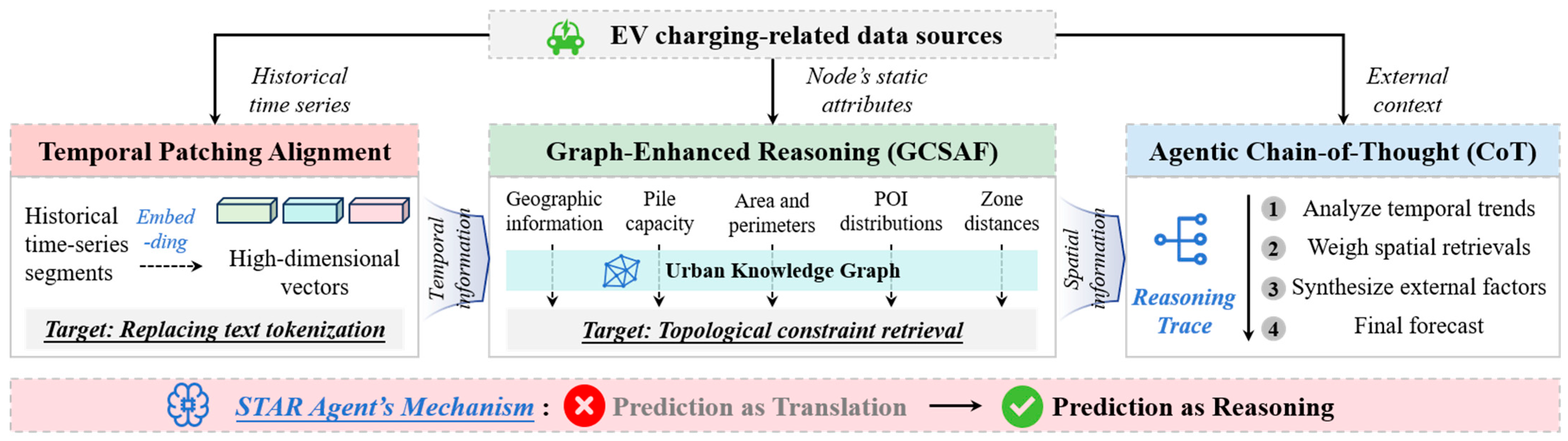
To address these challenges, this paper introduces STAR, a spatio-temporal agentic reasoning framework that shifts the forecasting paradigm from “Prediction as Translation” to “Prediction as Reasoning”. Unlike previous approaches that merely translate data into text, STAR empowers an LLM-based agent to perceive, retrieve, and reason about spatio-temporal dynamics before predicting. The term agentic denotes an autonomous system architecture governed by a structured perception–retrieval–reasoning–action workflow, distinguishing it from passive fine-tuned language models. Specifically, STAR acts as a spatio-temporal agent that actively perceives continuous numerical signals via temporal patching, interacts with an external topological environment through graph-conditioned spatial attention fusion (GCSAF), and executes “System 2” cognitive deliberation before committing to a final forecasting action. Its key idea is shown in Figure 1. The core contributions of this work are summarized as follows.

Firstly, to address the limitations of traditional text-based tokenization, the framework implements a temporal patching alignment strategy. By projecting historical time-series segments into high-dimensional vectors, this approach effectively preserves the mathematical fidelity of the data. Furthermore, this mechanism optimizes computational efficiency, enabling the LLM to process and reason over extended historical contexts without the precision loss associated with discrete text discretization.

Secondly, to explicitly model non-Euclidean spatial dependencies without relying on simplistic textual descriptions, the framework incorporates a GCSAF module integrating a domain-specific urban knowledge graph (UKG). Rather than executing discrete, tool-based text retrieval, this module leverages temporal patch representations as dynamic queries to calculate cross-attention over graph neural network (GNN)-encoded structural node embeddings, dynamically integrating spatial topological constraints into the LLM’s reasoning stream.

Finally, the architecture employs a “System 2” reasoning mechanism via an agentic chain-of-thought (CoT) inference engine [11]. The model is mandated to generate an explicit reasoning trace by systematically analyzing temporal trends, weighing spatial retrievals, and synthesizing external factors prior to deriving the final forecast. This process not only enhances predictive accuracy through logical self-correction but also yields human-readable explanations, thereby providing interpretable decision support for critical infrastructure management.

2. Related Works

The development of predictive models for EV charging demand has evolved from statistical analyses to sophisticated DL architectures, and most recently, to the exploration of LLMs [12]. This section reviews the literature across three pivotal dimensions: data-driven spatio-temporal forecasting, LLMs for time-series analysis, and the integration of graph reasoning in foundation models.

2.1. Data-Driven Spatio-Temporal Forecasting for EV Charging

Predicting EV charging demand is a complex spatio-temporal problem influenced by diverse factors such as traffic flow, weather, and charging pricing [13]. Early approaches primarily relied on statistical methods. For instance, ARIMA and Lasso regression models were widely employed to capture linear temporal patterns in charging records [14]. While these methods offer interpretability, they often struggle to model the non-linear dynamics and high volatility inherent in urban charging behaviors.

To address these limitations, DL techniques have become the dominant paradigm [15]. RNNs, particularly long short-term memory (LSTM) networks, were introduced to capture long-term temporal dependencies. For example, Wang et al. utilized LSTM blocks to predict short-term EV energy demand, demonstrating significant performance improvements over statistical baselines [16]. Similarly, Yi et al. applied LSTM and sequence-to-sequence to forecast charging demand by analyzing historical usage patterns [17].

However, temporal modeling alone is insufficient without considering spatial correlations [18]. Consequently, spatio-temporal neural networks have emerged as a powerful tool. Yu et al. established a foundation with STGCN by combining graph convolutions with gated temporal convolutions to extract spatio-temporal features [19]. Building on this, Kuang et al. introduced PIAST, a physics-informed approach that combines graph learning with attention mechanisms to capture correlations between charging occupancy and dynamic pricing [20]. Additionally, Tupayach et al. proposed a spatial-temporal graph convolutional recurrent network specifically for forecasting demand in energy markets [21].

Despite their success, these data-driven models face two critical limitations. First, they struggle to effectively align and fuse heterogeneous data sources due to the rigid structure of neural networks. Second, they typically function as black boxes with poor generalizability to unseen areas where historical data is scarce.

2.2. LLMs for Time-Series Analysis

The advent of LLMs, such as bidirectional encoder representations from Transformers [22], Sentence-T5 [23], and generative pre-trained Transformer (GPT) series [24], has revolutionized the handling of sequential data. Leveraging their massive pre-training on open-world corpora, LLMs exhibit exceptional capabilities in few-shot learning and reasoning.

A growing body of work has attempted to adapt LLMs for time-series forecasting [25]. Xue and Salim pioneered the prompt-based learning paradigm with PromptCast, which reformulates forecasting as a question-answering task by encoding numerical history into natural language prompts [26]. This approach allows the model to leverage semantic knowledge without modifying the architecture. Similarly, Gruver et al. demonstrated that LLMs can function as zero-shot forecasters by tokenizing time series into discrete strings, achieving competitive performance on continuous extrapolation tasks [27]. To further bridge the modality gap, Jin et al. proposed Time-LLM, a reprogramming framework that aligns time-series embeddings with the language space of frozen LLMs [28], while Lai et al. fine-tuned pre-trained models in Bert4st specifically for wind power forecasting [29].

In the specific context of EV charging, Qu et al. established the state-of-the-art (SOTA) with ChatEV [10]. It reformulates the prediction task into a text-to-text format, utilizing a fine-tuned Sentence-T5 model to align diverse features like coordinates and points of interest (POIs) within a unified semantic space. ChatEV incorporates spatial awareness by converting neighboring charging data into textual descriptions.

While ChatEV successfully introduces broad knowledge, it relies on a translation paradigm that converts high-precision numerical data into text strings. This tokenization process often leads to precision loss and is computationally inefficient for long-context reasoning. Furthermore, representing spatial topology merely as textual descriptions fails to capture the complex, non-Euclidean connectivity of urban road networks, limiting the model’s ability to reason about downstream EV charging demand.

2.3. Graph Learning and Reasoning in Foundation Models

To overcome the limitations of pure text-based approaches, recent research focuses on integrating structural knowledge into foundation models. Li et al. effectively inject spatio-temporal dependencies into LLMs with UrbanGPT by aligning graph structures with instruction tuning, showing promise in urban mobility tasks [30]. Similarly, Li et al. introduced FlashST, a prompt-tuning framework designed to enhance the efficiency of traffic prediction models [31].

Beyond structural alignment, enhancing the reasoning capability of agents is crucial. The CoT technique enables LLMs to decompose complex problems into sequential intermediate steps, significantly improving logical deduction. Liang et al. applied CoT in LLM-MPE to predict human mobility, using event features to guide the model’s thinking process [32]. Furthermore, role-playing strategies, where the LLM adopts a specific persona (e.g., “You are an expert in electric vehicle charging management”), have been shown to elicit better domain-specific performance [33]. Research has also explored using LLMs for explaining spatio-temporal graph behaviors to improve interpretability [34].

Although methods like UrbanGPT integrate graphs, and approaches like LLM-MPE utilize CoT, there remains a gap in establishing a unified agentic framework for EV charging demand prediction. Existing models either lack explicit topological retrieval or separate the reasoning process from the spatial graph structure. Our proposed STAR framework addresses this by combining graph-enhanced retrieval with agentic reasoning, moving beyond simple translation to interpretable, logic-driven forecasting. To systematically summarize existing methodologies and explicitly highlight the architectural innovations of STAR,

Table 1. Systematic comparison of representative forecasting paradigms and the proposed STAR framework.

Category	Representative Methods	Temporal Modeling and Numerical Precision	Spatial Dependency Modeling	Decision Process and Interpretability	Cross-Zone/Zero-Shot Transferability
Statistical methods	ARIMA and Lasso [14]	Linear autoregression; highly constrained non-linear fitting	None (isolated spatial units)	Black-box/Linear coefficients; no causal deduction	Poor (requires complete retraining per series)
Deep Learning and Spatio-Temporal GNNs	STGCN [19], PIAST [20]	Recurrent/convolutive feature extraction; continuous numeric space	Predefined static adjacency matrices or localized graph convolutions	Black-box latent mappings; lacks human-readable explanations	Limited (rigidly tied to fixed source graph topology)
LLM as Translation	PromptCast [26], LLMTIME [27], ChatEV [10]	Text tokenization of numbers; prone to precision loss and context window expansion	Flattened textual spatial descriptions; misses non-Euclidean topology	Direct end-to-end prompt completion; no intermediate reasoning traces	Moderate (open-world semantic transfer, but sensitive to textual drift)
Foundation Models with Structural Alignment	UrbanGPT [30], FlashST [31], LLM-MPE [32]	GNN-to-LLM instruction tuning or linear reprogramming	Graph-structure alignment; static topological projection	Implicit feature alignment or single-event CoT	Moderate to good (spatial alignment across domains)
Proposed Solution	STAR	Temporal patching alignment; preserves mathematical fidelity without context explosion	Dynamic topological retrieval via GCSAF over Urban Knowledge Graph	Agentic CoT inference engine; generates explicit, verifiable reasoning traces	High (robust zero-shot and few-shot spatial transfer via invariant retrieval policy)

provides a comprehensive multi-dimensional comparison between representative prior paradigms and our proposed framework.

3. Problem Definition and Methodology

This section articulates the technical realization of the proposed STAR framework. First, the mathematical formulation of the EV charging demand prediction problem is established, followed by an overview of the STAR agent’s overarching architecture. Subsequently, three core innovations driving the framework are detailed: the temporal patching alignment mechanism, the GCSAF module, and the CoT inference engine. Finally, the optimization objectives and the training paradigm utilized to fine-tune the agent are outlined.

3.1. Mathematical Formulation and General Framework

3.1.1. Urban Knowledge Graph

To capture non-Euclidean spatial dependencies across city-wide charging networks, we construct the UKG $\mathcal{G}=\left(\mathcal{V},\mathcal{E},\mathrm{A}\right)$.

Nodes ($\mathcal{V}$): Each node $v_i\in \mathcal{V}$ represents one of the investigated traffic zones.

Edges ($\mathcal{E}$) and adjacency structure: We construct a directed, weighted spatial graph based on road-network physical distance and topological connectivity. An edge $e_{ij}=\left(v_i,v_j\right)\in \mathcal{E}$ indicates spatial reachability from zone $v_j$ to zone $v_i$. Edge existence is thresholded by a physical distance cutoff $D_{\max }=10 \mathrm{km}$, beyond which inter-zone spatial spillover becomes negligible. Physically, 10 km corresponds to the typical urban cruising threshold within a 15–20 min driving radius in dense traffic. Setting $D_{\mathrm{m}\mathrm{a}\mathrm{x}}<5 \mathrm{km}$ causes excessive graph sparsity that misses cascading traffic shifts, whereas $D_{\mathrm{m}\mathrm{a}\mathrm{x}}>20 \mathrm{km}$ incurs spatial over-smoothing and noise from functionally decoupled distant districts.

Edge weights (${\mathit{a}}_{\mathit{i}\mathit{j}}$): The edge weight $a_{ij}$ models spatial proximity using a Gaussian kernel based on road-network travel distance $d_{ij}$ [35]:

$$a_{ij}=\left\{\begin{array}{cc}\exp \left(-{\left({\displaystyle \frac{d_{ij}}{\sigma }}\right)}^2\right),& \mathrm{if} d_{ij}\le D_{\max } \mathrm{and} i\ne j\\ 0,& \mathrm{otherwise}\end{array}\right.$$

(1)

where $\sigma$ denotes the standard deviation of road distances across all pairs.

Static attributes ($\mathcal{A}$): Each node $v_i$ is initialized with static feature vector ${\mathrm{A}}_i$, comprising geographic coordinates, total pile capacity, zone perimeter, area, and POI distribution vectors.

3.1.2. Problem Definition

The EV charging demand prediction task is formulated as estimating future demand based on historical observations. We define the following key variables:

Historical time series ($\mathit{X}$): Let $x_{i,t}\in \mathbb{R}$ denote the dynamic charging-related variables of traffic zone $i$ at time step $t$. The system-wide historical input over a lookback window $L$ is defined as a tensor $X=[X_{t-L+1},\dots ,X_t]\in {\mathbb{R}}^{N\times L\times C}$, where $C$ is the number of input channels.

External context ($\mathcal{C}$): A set of textual descriptions describing environmental factors at time $t$, such as weather reports, including ambient temperature and relative humidity, and day types, including workdays or holidays.

Reasoning trace ($\mathcal{R}$): A sequence of natural language tokens generated by the agent that explicitly describes the logical steps taken to arrive at a prediction.

Unlike traditional deterministic models that learn a mapping $f:(X,\mathcal{G})\to Y$, STAR formulates the problem as a generative reasoning task. Given the historical context $X$, the UKG $\mathcal{G}$, and external context $\mathcal{C}$, the goal is to maximize the joint probability of generating the reasoning trace $\mathcal{R}$ and the future demand $Y\in {\mathbb{R}}^{N\times H}$ for the next $H$ horizons:

$${\mathcal{L}}_{\mathrm{STAR}}=\sum _t\mathrm{l}\mathrm{o}\mathrm{g}{P}_{\theta }(Y_{t+1:t+H},{\mathcal{R}}_t\mid X_{t-L+1:t},\mathcal{G},{\mathcal{C}}_t)$$

(2)

where $\theta$ represents the learnable parameters of the LLM and the alignment encoders.

3.1.3. General Framework

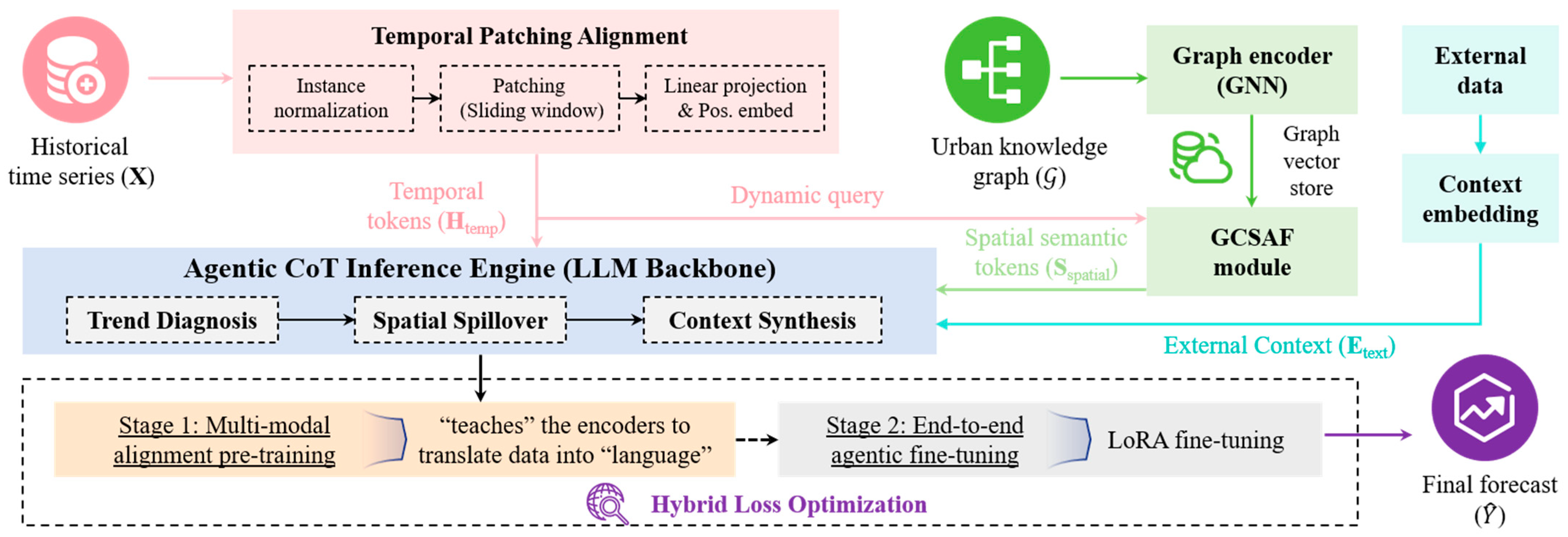
The STAR framework orchestrates a seamless, cascaded information flow that integrates temporal precision, spatial topology, and logical reasoning to solve the generative forecasting task, as shown in Figure 2. The process initiates with the temporal patching alignment module, which transforms the high-frequency historical time series $X$ into a sequence of dense temporal embeddings. These embeddings serve as the foundational numerical input, preserving mathematical fidelity while compressing the context length. Crucially, these temporal tokens function as dynamic queries for the GCSAF module, which retrieves relevant topological embeddings from the UKG $\mathcal{G}$, thereby enriching the agent’s context with non-Euclidean spatial dependencies that purely temporal data cannot capture. Finally, the agentic CoT inference engine ingests these fused temporal and spatial modalities, utilizing a “System 2” reasoning mechanism to synthesize the heterogeneous information. This core module first generates an explicit reasoning trace to articulate the logical deduction of demand fluctuations before deterministically outputting the final predicted demand values. From an agentic systems perspective, STAR realizes an autonomous closed-loop cognitive workflow by seamlessly orchestrating perception, retrieval, reasoning, and action. Specifically, it actively perceives multi-channel physical time series as dense semantic states, dynamically retrieves non-Euclidean topological dependencies from an external UKG, deliberates via an agentic CoT engine to synthesize multi-modal causal factors, and ultimately commits to a forecasting action that maps the synthesized cognitive state to precise demand predictions.

3.2. Temporal Patching Alignment

A fundamental bottleneck in applying LLMs to time-series forecasting lies in the modality misalignment between continuous numerical data and the discrete token space of pre-trained text models. Previous approaches, such as the translation paradigm adopted in ChatEV, typically resort to tokenizing time-series data into character strings (e.g., converting the float 0.235 into the sequence [‘0’, ‘.’, ‘2’, ‘3’, ‘5’]). This textualization process not only fragments the intrinsic mathematical continuity of the signal but also results in an exorbitant expansion of the context window, severely limiting the model’s ability to model long-range dependencies. To resolve this, the STAR framework introduces a temporal patching alignment mechanism, which preserves numerical precision by treating local temporal segments as high-dimensional semantic units rather than discrete text tokens.

Formally, given the multivariate historical time series $X\in {\mathbb{R}}^{N\times L\times C}$ for $N$ traffic zones over a lookback window $L$ with $C$ channels, we first employ instance normalization [36] to mitigate the distribution shift problem prevalent in non-stationary EV charging data. Instead of processing individual time steps $x_t$ as scalars, we aggregate adjacent time steps into segments, referred to as patches. This is achieved through a sliding window operation where the input series $x^{\left(i\right)}\in {\mathbb{R}}^L$ for the $i$-th variate is unfolded into a sequence of patches ${\mathcal{P}}^{\left(i\right)}\in {\mathbb{R}}^{M\times P}$. Here, $P$ denotes the patch length, and $S$ represents the non-overlapping stride. The number of patches $M$ generated for the input window is determined by [37]:

$$M=⌊{\displaystyle \frac{L-P}{S}}⌋+2$$

(3)

where the final sequence is padded to ensure dimensional consistency. By clustering local semantic information such as a specific charging peak or a sudden drop trend into a unified sub-series, this patching operation reduces the input sequence length from $L$ to $M$. Consequently, it significantly optimizes the computational complexity of the subsequent attention mechanisms.

To align these continuous numerical patches with the semantic space of the LLM, we employ a trainable linear projection layer. Unlike standard tokenizers that look up static embeddings from a vocabulary, our projection layer dynamically maps the dense numerical vectors into the LLM’s high-dimensional embedding space $d_{model}$. For the $k$-th patch $p_k^{\left(i\right)}$ of traffic zone $i$, the projected embedding $e_k^{\left(i\right)}\in {\mathbb{R}}^{d_{model}}$ is computed as:

$$e_k^{\left(i\right)}=p_k^{\left(i\right)}{W}_p+b_p$$

(4)

where $W_p\in {\mathbb{R}}^{P\times d_{model}}$ and $b_p\in {\mathbb{R}}^{d_{model}}$ are the learnable weights and biases of the alignment projector.

Finally, since the pure linear projection is permutation-invariant and fails to capture the sequential order of the patches, we inject a learnable positional embedding matrix $W_{pos}\in {\mathbb{R}}^{M\times d_{model}}$ into the projected patch sequence. For the $k$-th temporal patch of traffic zone $i$, its position-aware patch token ${\tilde{e}}_k^{\left(i\right)}\in {\mathbb{R}}^{d_{model}}$ is constructed as:

$${\tilde{e}}_k^{\left(i\right)}=e_k^{\left(i\right)}+w_k^{pos}$$

(5)

where $w_k^{pos}\in {\mathbb{R}}^{d_{model}}$ represents the $k$-th row vector of $W_{pos}$. The aggregated temporal representation tensor for zone $i$ is obtained by stacking these tokens $H_{temp}^{\left(i\right)}={\left[{\tilde{e}}_1^{\left(i\right)},{\tilde{e}}_2^{\left(i\right)},\dots ,{\tilde{e}}_M^{\left(i\right)}\right]}^T\in {\mathbb{R}}^{M\times d_{model}}$.

By treating time-series patches as semantic tokens, this mechanism allows the STAR agent to perceive temporal dynamics with the same fidelity as natural language words, effectively bridging the modality gap without the precision loss associated with textual discretization.

3.3. Spatial Context Fusion Module

While the temporal patching mechanism effectively captures the historical trends of individual traffic zones, it treats each traffic zone as an isolated entity, ignoring the complex, non-Euclidean spatial dependencies that govern urban traffic flows. Traditional approaches often rely on flattening these spatial relationships into textual descriptions, which fails to convey the structural propagation of demand, such as how a traffic bottleneck at an upstream node cascades to downstream traffic zones. To overcome this spatial shallowness, the STAR framework incorporates a GCSAF module. This module empowers the agent to actively interrogate the UKG $\mathcal{G}$, transforming static topological constraints into dynamic, context-aware prompts that guide the reasoning process.

The perception phase of GCSAF begins with the encoding of the UKG into a latent vector space. We employ a GNN as the structural encoder to aggregate local neighborhood information [38]. For every node $v_i\in \mathcal{V}$, its initial state $h_i^{\left(0\right)}$ is initialized with static attributes ${\mathcal{A}}_i$. We then apply a multi-layer message-passing mechanism to propagate information across the network. At the $l$-th layer, the structural embedding $h_i^{\left(l\right)}$ for node $v_i$ is updated by aggregating features from its local topological neighbors $j\in \mathcal{N}\left(i\right)$ alongside its self-state [39]:

$$h_i^{\left(l+1\right)}=\sigma \left(W^{\left(l\right)}{h}_i^{\left(l\right)}+\sum _{j\in \mathcal{N}\left(i\right)}{a}_{ij}{W}^{\left(l\right)}{h}_j^{\left(l\right)}\right)$$

(6)

where $W^{\left(l\right)}\in {\mathbb{R}}^{d_{l+1}\times d_l}$ represents the learnable weight matrix at the $l$-th layer, $\sigma \left(\cdot \right)$ denotes a non-linear ReLU activation function, and $a_{ij}$ represents the normalized edge weight defined in Equation (1). After $K$ layers of aggregation, we obtain the final structural embedding $H_{\mathrm{graph}}=\{h_1^{\left(K\right)},\dots ,h_N^{\left(K\right)}\}$, which encapsulates the high-order topological context of the entire network. These embeddings constitute the graph vector store, serving as the knowledge base for the subsequent retrieval operation.

The core innovation of the GCSAF module lies in the retrieval mechanism, which links the temporal dynamics to spatial structures. Unlike standard retrieval-augmented generation (RAG) which retrieves text chunks based on semantic similarity, our GCSAF retrieves topological features based on the current temporal state. We treat the aligned temporal representation $H_{\mathrm{temp}}^{\left(i\right)}$ of traffic zone $i$ as the query, and the structural embeddings $H_{\mathrm{graph}}$ as the key and value. To identify which spatial neighbors are most relevant to the current charging trend, we employ a cross-attention retrieval mechanism. The retrieved spatial context $c_{\mathrm{spatial}}^{\left(i\right)}$ is computed as [40]:

$$c_{\mathrm{spatial}}^{\left(i\right)}=\mathrm{Attention}(Q_i,K,V)=\mathrm{softmax}\left({\displaystyle \frac{{\left(H_{\mathrm{temp}}^{\left(i\right)}{W}_Q\left)\right(H_{\mathrm{graph}}{W}_K\right)}^T}{\sqrt{d_k}}}\right)\times \left(H_{\mathrm{graph}}{W}_V\right)$$

(7)

where $W_Q,W_K,W_V$ are projection matrices. This operation effectively allows the STAR agent to dynamically retrieve a weighted summary of the network topology that is most pertinent to the current time step.

Finally, to fuse this retrieved topological knowledge into the LLM’s reasoning stream, the context vector $c_{\mathrm{spatial}}^{\left(i\right)}$ is projected into the model’s dimension $d_{model}$ via a linear adapter. This results in a sequence of spatial semantic tokens $S_{\mathrm{spatial}}^{\left(i\right)}$.

3.4. Agentic CoT Inference Engine

Having aligned the continuous temporal signals and discrete topological features into a unified semantic space, the final component of the STAR framework is the agentic CoT inference engine. Unlike conventional forecasting models that function as black boxes mapping inputs directly to outputs via implicit feature interactions, our engine is designed to emulate “System 2” cognitive processing. It mandates the agent to explicitly articulate the intermediate logical steps by analyzing trends, synthesizing spatial contexts, and weighing external factors before committing to a final numerical prediction. This mechanism not only enhances interpretability for grid operators but also improves prediction accuracy by allowing the model to self-correct via intermediate reasoning states.

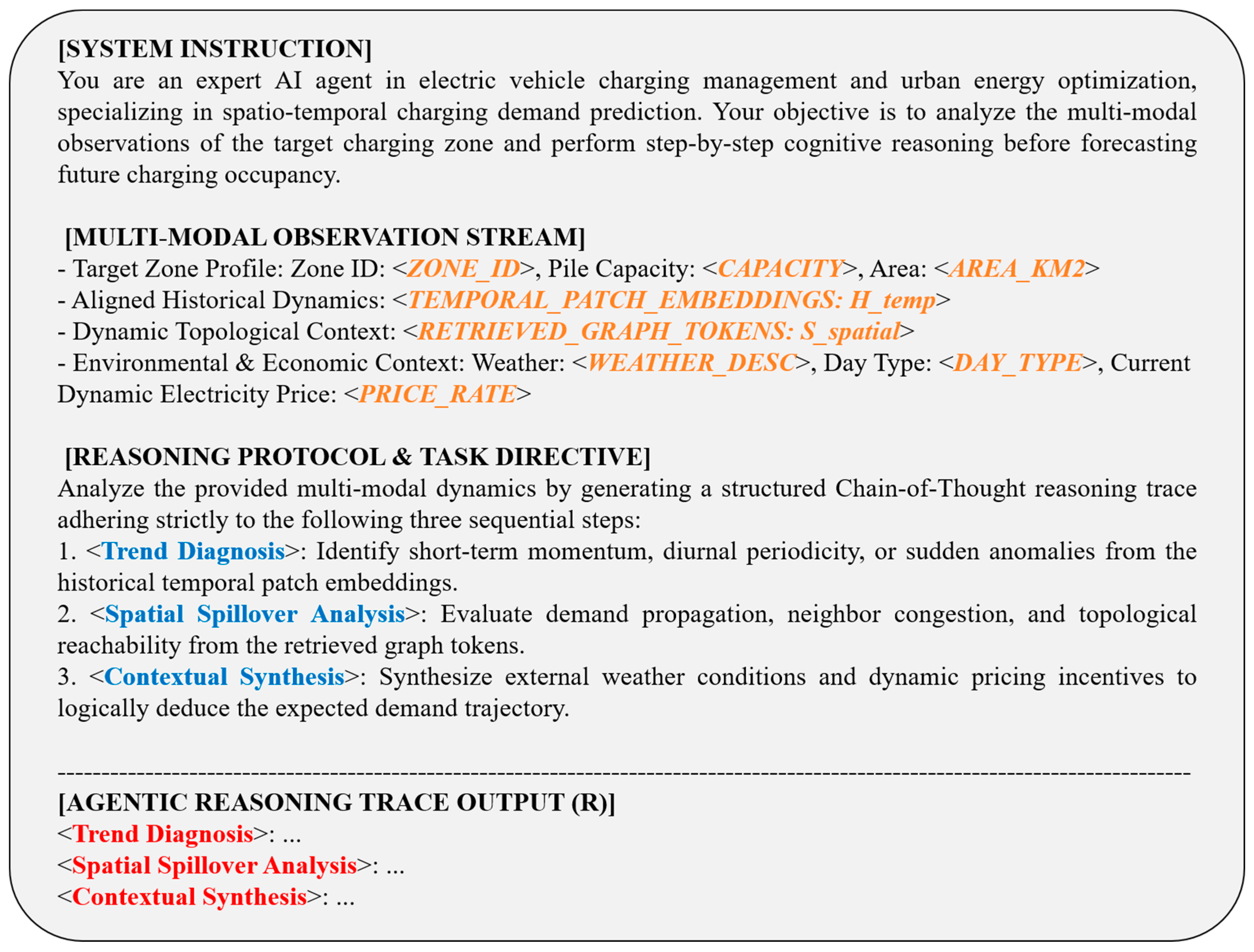
The inference process begins by constructing a composite prompt structure that orchestrates the multi-modal inputs. We define a meta-instruction ${\mathcal{I}}_{sys}$ that assigns the specific role to the LLM (namely, “You are an expert in electric vehicle charging management, who is good at charging demand prediction…”) and enforces the reasoning protocol. The complete input sequence $Z_{in}$ fed into the LLM backbone is a concatenation of the system instruction, the aligned temporal tokens from Section 3.2, the retrieved spatial tokens from Section 3.3, and the embeddings of external textual context $E_{\mathrm{text}}$:

$$Z_{in}=\mathrm{Concat}({\mathcal{I}}_{sys},H_{\mathrm{temp}},S_{\mathrm{spatial}},E_{\mathrm{text}})$$

(8)

This composite embedding ensures that the agent has simultaneous access to “what happened” (temporal), “where it happened” (spatial), and “environmental conditions” (external) within its attention window. To provide an operational view of this multi-modal orchestration and ensure complete technical reproducibility, the exact structure of the agentic prompt template and its sequential CoT directive are illustrated in Figure 3.

The core generative process is formulated as a conditional probability maximization problem. Unlike ChatEV which directly maximizes the probability of the target value sequence, STAR decomposes the generation into two sequential stages: the reasoning trace and the forecast. The model first autoregressively generates a sequence of reasoning tokens $\mathcal{R}=\left\{r_1,r_2,\dots ,r_K\right\}$, where each token $r_k$ is strictly conditioned on the input sequence $Z_{in}$ and all previously generated preceding tokens $r_{<k}=\left\{r_1,\dots ,r_{k-1}\right\}$:

$$P_{\theta }\left(\mathcal{R}|Z_{in}\right)={\displaystyle \prod _{k=1}^K}{P}_{\theta }\left(r_k\mid Z_{in},r_{<k}\right)$$

(9)

where $P_{\theta }\left(r_k\mid Z_{in},r_{<k}\right)$ denotes the conditional probability predicted by the LLM backbone parameterized by $\theta$ at the $k$-th decoding step.

During this phase, the agent is guided to perform several specific cognitive tasks. First, it conducts trend identification by identifying periodicity or sudden spikes in the temporal patches. Second, it executes spatial causality analysis by interpreting retrieved graph features. Finally, it performs contextual synthesis to adjust expectations based on external events.

Following the termination of the reasoning trace, the agent proceeds to generate the final prediction. To ensure numerical validity and facilitate downstream integration, we employ a prediction token head. Rather than generating loose text, the model projects the final hidden state $h_{final}$ after the reasoning trace into the forecast horizon dimension $H$:

$$\widehat{\mathbf{Y}}={\mathrm{Linear}}_{\varphi }\left(h_{final}\right);h_{final}={\mathrm{LLM}}_{\theta }(Z_{in},\mathcal{R})$$

(10)

Here, $\widehat{\mathbf{Y}}\in {\mathbb{R}}^H$ represents the predicted charging demand for the next $H$ time steps. By conditioning the final prediction on the explicit reasoning trace $\mathcal{R}$, the STAR framework ensures that the quantitative forecast is logically consistent with the qualitative analysis, effectively bridging the gap between interpretability and accuracy.

3.5. Optimization and Training Paradigm

Training the STAR framework presents a unique challenge, requiring a balance between the discrete, probabilistic nature of text generation and the continuous, deterministic nature of regression. To address this, we adopt a two-stage instruction tuning paradigm. This strategy first aligns the heterogeneous modalities with the LLM’s semantic space, and subsequently fine-tunes the agent’s reasoning capabilities in an end-to-end manner.

Stage 1: Multi-modal alignment pre-training. In the initial phase, our primary objective is to bridge the modality gap between the numerical encoders and the pre-trained LLM backbone. We freeze the parameters of the LLM, denoted as ${\Theta }_{\mathrm{LLM}}$, to preserve its pre-existing reasoning and linguistic capabilities. We solely optimize the parameters of the temporal patching projector and the graph encoder weights. The goal is to ensure that the projected temporal embeddings $H_{\mathrm{temp}}$ and spatial tokens $S_{\mathrm{spatial}}$ carry sufficient semantic information for the LLM to interpret. We employ a standard regression loss ${\mathcal{L}}_{\mathrm{align}}$ on the prediction head, forcing the encoders to extract features that are predictive of the ground truth demand $Y_{gt}$:

$${\mathcal{L}}_{\mathrm{align}}={\displaystyle \frac{1}{N\times H}}{\displaystyle \sum _{i=1}^N}{\left|\right|{\widehat{Y}}_i-Y_{gt,i}\left|\right|}_2^2$$

(11)

where ${\widehat{Y}}_i$ is the output of the prediction head derived from the frozen LLM’s hidden states. This stage effectively teaches the encoders to translate raw data into a language the LLM can understand.

Stage 2: End-to-end agentic fine-tuning. Once the modalities are aligned, the second stage focuses on empowering the agent to perform explicit reasoning. We employ parameter-efficient fine-tuning technique low-rank adaptation (LoRA) [41] and train the entire framework jointly. We employ LoRA rather than full fine-tuning or prompt-based parameter-efficient fine-tuning alternatives like prefix tuning. Specifically, full fine-tuning on specialized numerical-text datasets risks catastrophic forgetting of the pre-trained LLM’s open-world deductive capabilities, while prefix tuning prepends virtual prompt tokens that undesirably occupy the bounded attention sequence window and interfere with multi-modal token representations. In contrast, LoRA applies lightweight rank-decomposition updates directly to the attention projection weights, preserving foundational reasoning priors, avoiding sequence length inflation, and enabling zero-latency weight merging for real-time dispatch deployment.

The optimization objective is a hybrid loss function that combines causal language modeling for the reasoning trace and prediction error for the numerical forecast. Let ${\mathcal{R}}_{gt}$ denote the ground-truth reasoning trace, which can be distilled from a teacher model of GPT-4 [42], and $Y_{gt}$ denote the actual future demand. The total loss ${\mathcal{L}}_{\mathrm{total}}$ is defined as:

$${\mathcal{L}}_{\mathrm{total}}=\lambda {\mathcal{L}}_{\mathrm{reason}}+(1-\lambda ){\mathcal{L}}_{\mathrm{pred}}$$

(12)

The reasoning loss ${\mathcal{L}}_{\mathrm{reason}}$ minimizes the negative log-likelihood of generating the correct reasoning tokens $r_k$ given the input context $Z_{in}$ [43]:

(13)

The prediction loss ${\mathcal{L}}_{\mathrm{pred}}$ ensures the final numerical output is accurate:

$${\mathcal{L}}_{\mathrm{pred}}={\displaystyle \frac{1}{H}}\left|\right|{\mathrm{Linear}}_{\varphi }\left(h_{final}\right)-Y_{gt}{\left|\right|}_2^2$$

(14)

In the above equations, $\theta$ and $\varphi$: denote the trainable parameters of the LLM backbone and the linear projection head, respectively. $P_{\theta }\left(r_k\mid {\mathbf{Z}}_{\mathrm{in}},r_{<k}\right)$ denotes the conditional probability of predicting the $k$-th reasoning token given the input context and preceding tokens. $h_{\mathrm{final}}$ is the final hidden state representation of the LLM backbone generated upon completing the reasoning trace. $\lambda \in [0, 1]$ is a hyperparameter balancing the trade-off between qualitative reasoning interpretability and quantitative numerical accuracy. Because discrete language token cross-entropy naturally exhibits a higher loss magnitude than normalized continuous regression error, $\lambda$ balances gradient magnitudes across the two multi-task objectives.

We utilize the AdamW optimizer for minimizing ${\mathcal{L}}_{\mathrm{total}}$, employing a cosine annealing learning rate scheduler to stabilize the convergence of the multi-task objective. By optimizing this hybrid loss, STAR learns to produce forecasts that are not only numerically precise but also logically grounded in the generated reasoning path.

To supervise the autoregressive reasoning generation during Stage 2, we employ a teacher-distilled rationale mechanism. To prevent ambiguous terminology, we explicitly designate ${\mathcal{R}}_{\mathrm{gt}}$ as the teacher-distilled synthetic reasoning trace, generated offline via GPT-4. A fundamental prerequisite of our distillation pipeline is the complete isolation of target labels. During the generation of ${\mathcal{R}}_{\mathrm{gt}}$, the teacher model GPT-4 is provided exclusively with historical time-series patches $X_{t-L+1:t}$, external textual context ${\mathcal{C}}_t$, and retrieved dynamic spatial neighbor attributes from $\mathcal{G}$. Crucially, the future ground-truth demand values $Y_{t+1:t+H}$ are strictly withheld from the teacher model. This setup guarantees that ${\mathcal{R}}_{\mathrm{gt}}$ represents a pure forward deductive reasoning path based solely on causal historical evidence, completely eliminating the risk of label leakage during fine-tuning.

The offline trace dataset consists of 15,000 carefully curated spatio-temporal reasoning samples extracted across representative traffic zones, generated by supplying GPT-4 with an exact system prompt that enforces a structured three-stage rationale template comprising temporal trend diagnosis, spatial neighbor spillover analysis, and external factor synthesis. To ensure high fidelity and quality, these generated traces undergo a rigorous two-step automated filtering process where a structural completeness check instantly discards any traces missing any of the three mandatory reasoning stages, and a quantitative consistency verification cross-references qualitative claims, such as expecting a demand surge during morning rush hour, with the direction of historical moving averages to remove traces containing hallucinatory contradictions like predicting an increase during a historical drop without an external rationale.

4. Validation

To empirically validate the effectiveness of the proposed STAR framework, we conduct extensive experiments comparing it against SOTA baselines. We specifically aim to investigate whether the shift from a translation paradigm to an agentic reasoning paradigm yields superior accuracy and generalizability in EV charging demand prediction.

4.1. Experimental Setup

4.1.1. Datasets

We evaluate our model using ST-EVCDP dataset collected from Shenzhen, China, which serves as a standard for large-scale urban charging analysis [44]. This dataset aggregates real-time charging occupancy information from $N=\mathrm{18,061}$ public EV charging piles distributed across $247$ traffic zones. The data spans a period of 30 days from 19 June to 18 July 2022, with a fine-grained time interval of $\Delta t=5$ min. The 30-day continuous period at a fine-grained 5 min sampling interval yields 8640 consecutive timestamps across 247 traffic zones, generating over 2.13 million spatio-temporal data points. Following the established benchmark protocol in ChatEV [10], we adopt a chronological split for training, validation, and testing, which are partitioned into 70%, 10%, and 20% of the dataset, respectively. This chronological partitioning strictly preserves temporal causality and eliminates data leakage. Because the training partition spans multiple complete weekly diurnal cycles and weather conditions, it provides sufficient high-frequency sequential transitions to optimize short-to-medium-term forecasting models while ensuring a direct and standardized comparison against state-of-the-art baselines. Crucially for our multi-modal approach, ST-EVCDP includes a rich set of heterogeneous features, comprising dynamic pricing schemes, geographical coordinates, road length density, POI distributions, etc. 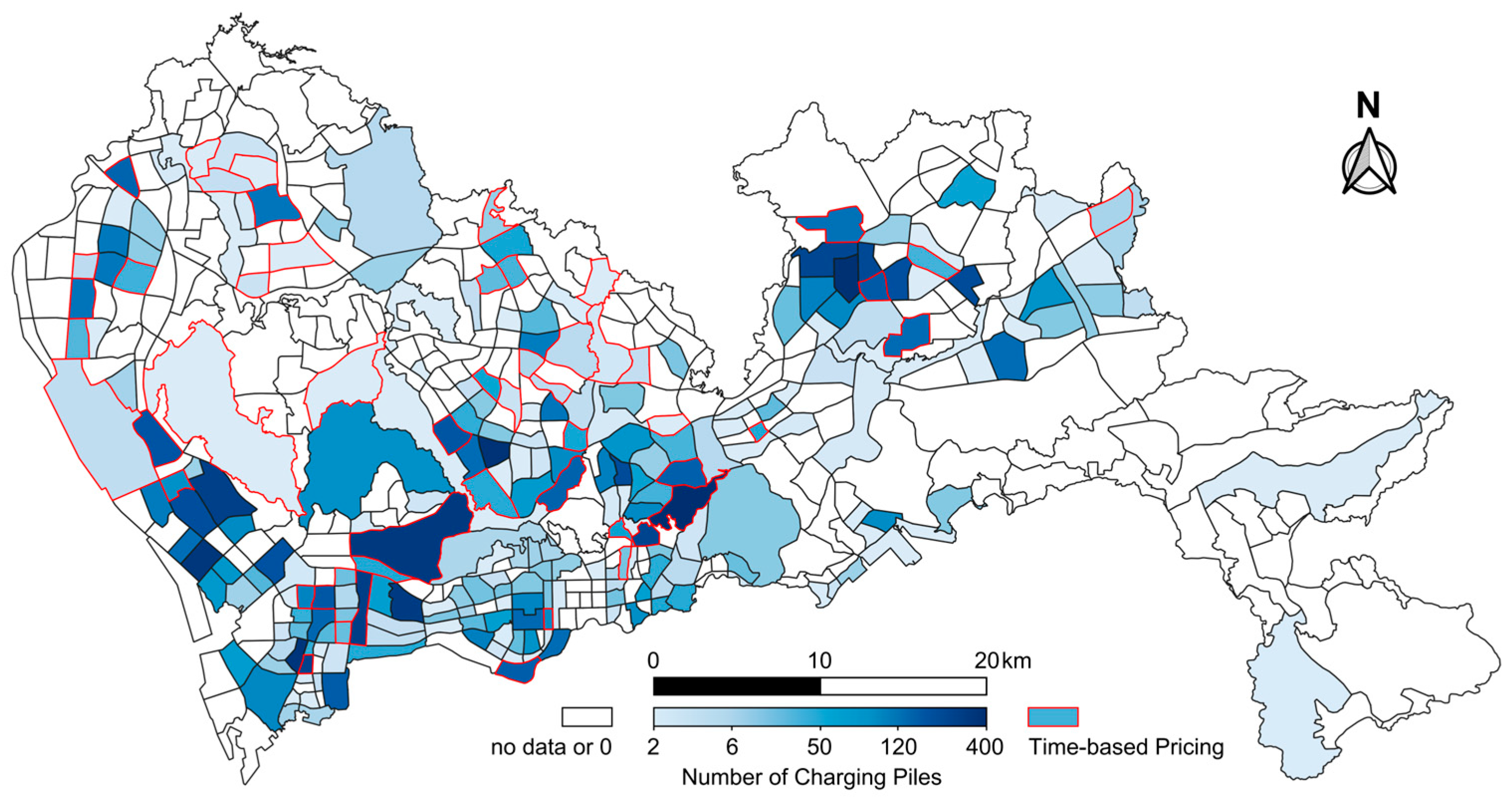Figure 4 shows the spatial distribution of the 18,061 public EV charging piles in ST-EVCDP.

In the STAR framework, the heterogeneous data sources from the ST-EVCDP dataset are rigorously stratified into three distinct input modalities to facilitate multi-modal alignment and agentic reasoning. First, the historical time series component encapsulates the continuous numerical dynamics of the system. This category includes the charging occupancy ratio, charging duration, and charging volume, which constitute the primary multivariate tensor $X$ representing the system’s fluctuating state. Additionally, economic incentives such as electricity price and service fee are integrated into this temporal stream as dynamic covariates, capturing the time-variant costs that influence user demand. Second, the external context serves as a semantic anchor for environmental situational awareness. Weather data is processed not as numerical scalars but as textual descriptions, forming the context set $\mathcal{C}$ that allows the LLM to reason about environmental impacts on charging behavior and day type. Finally, node’s and edge’s static attributes provide the structural foundation for the UKG. This category aggregates spatially invariant features, including geographic information to define topological connectivity, and physical constraints such as pile capacity and the area and perimeters of the zone. Furthermore, POI distributions and zone distances are encoded as static node and edge attributes, enabling the GCSAF module to retrieve functional dependencies between distinct traffic zones. The mapping of ST-EVCDP data items to STAR input modalities is shown in

Table 2. Mapping of ST-EVCDP data items to STAR framework input modalities.

STAR Input Modality	UrbanEV Data Items	Computational Role
Historical Time Series ($X$)	Charging occupancy ratio	Processed via temporal patching alignment to preserve numerical precision and capture dynamic trends.
	Charging duration
	Charging volume
	Electricity price and service fee
External Context ($\mathcal{C}$)	Weather data	Textual descriptions to provide semantic environmental awareness.
	Day type
Node’s Static Attributes ($\mathcal{A}$)	Geographic information (Longitude/Latitude)	Used to construct the UKG and facilitate topological retrieval via GCSAF.
	Pile capacity
	The area and perimeters of the zone
	POI distributions
	Zone distances

.

4.1.2. Training Details

The proposed STAR framework is implemented using the PyTorch library 2.9.0., leveraging the pre-trained Flan-T5-Base architecture as the underlying reasoning backbone [45]. All experiments were executed on a high-performance Linux workstation equipped with dual NVIDIA GeForce RTX 3090Ti GPUs, utilizing data parallelism to optimize computational efficiency. The architectural components, training hyperparameters, and optimization settings of the STAR framework are thoroughly standardized as follows. The temporal patch length $P$ is set to $4$ with a non-overlapping stride $S=4$, yielding $M=3$ temporal patches. The linear projector projects continuous patches into a high-dimensional embedding space with $d_{\mathrm{model}}=768$ to match the Flan-T5-Base backbone. The UKG structural encoder is implemented using a 2-layer graph attention network with $K=2$ layers and $4$ spatial attention heads per layer. The output graph embedding dimension $d_{\mathrm{graph}}$ is $256$. The GCSAF cross-attention retrieval mechanism uses $8$ parallel attention heads. The maximum sequence length for textual prompt inputs is capped at 512 tokens, while the maximum generation length for CoT reasoning traces is set to 128 tokens. Stage 1 multi-modal alignment is trained for 15 epochs with a constant learning rate of $5\times {10}^{-4}$, where the LLM backbone remains frozen.

During Stage 2 agentic fine-tuning, LoRA is applied to the query and value projection matrices ($W_q,W_v$) of all self-attention layers with a rank $r=16$, scaling factor $\alpha =32$, and LoRA dropout rate $p_{\mathrm{drop}}=0.1$. Both alignment and fine-tuning stages are optimized using AdamW (${\beta }_1=0.9,{\beta }_2=0.999$, weight decay ${\lambda }_{\mathrm{decay}}=0.01$). The initial learning rate is set to $1\times {10}^{-4}$ with a cosine annealing scheduler decaying to $1\times {10}^{-6}$. Models are trained with a batch size of $32$ for a maximum of $50$ epochs. An early stopping mechanism with patience of $8$ epochs is enforced based on the validation loss to prevent overfitting. A linear learning rate warmup is applied for the first 5% of the total training steps, and gradients are clipped to a maximum $L_2$-norm of 1.0 to ensure numerical stability. During the inference phase, greedy decoding is utilized for deterministic CoT trace generation with a temperature of 0. The hyperparameter $\lambda$ in the hybrid loss is set to 0.3, determined via grid search over $\left\{0.1, 0.3, 0.5, 0.7\right\}$ on the validation set. Smaller values ($\lambda \le 0.1$) weaken the cognitive regularization of CoT traces, while larger values ($\lambda \ge 0.7$) over-prioritize textual generation at the expense of numerical regression precision.

4.1.3. Baselines

To rigorously validate the efficacy of our approach, we benchmark STAR against a comprehensive suite of baselines, systematically categorized into traditional statistical and DL methodologies as well as emerging LLM-based forecasting paradigms. Within the traditional domain, we employ classical statistical models such as ARIMA and Lasso, alongside DL architectures like Fourier convolutional neural network (FCNN) and LSTM, to evaluate fundamental temporal modeling capabilities. Furthermore, to strictly account for spatial dependencies, we incorporate a diverse array of spatio-temporal GNNs, such as GCN-LSTM, STGCN, HSTGCN, PIAST, and graph wavenet (GWNet). These models leverage mechanisms ranging from graph convolutions to adaptive adjacency matrices to capture intricate spatio-temporal correlations.

In the realm of LLM-empowered forecasting, we compare against four distinct paradigms. We employ PromptCast and LLMTIME as baselines for zero-shot prompt-based forecasting, treating the prediction task as a direct question-answering problem or continuous extrapolation without specific domain adaptation. Time-LLM represents the foundation model approach, utilizing cross-modality alignment to reprogram LLMs for general time-series tasks. Most critically, we compare STAR against ChatEV, the current SOTA model which reformulates prediction as a text-to-text translation task using a fine-tuned Sentence-T5 backbone.

4.1.4. Evaluation Metrics

The predictive performance is evaluated using three standard metrics, including root mean squared error (RMSE), mean absolute error (MAE), and mean absolute percentage error (MAPE). Depending on the specific focus and context of different experimental scenarios, a pertinent subset or the full combination of these metrics is reported for concise and targeted evaluation. The metrics are defined as follows:

$$\mathrm{RMSE}=\sqrt{{\displaystyle \frac{1}{H\times N}}{\displaystyle \sum _{i=1}^H}(Y_{t,i}-{\widehat{Y}}_{t,i}{)}^2}$$

(15)

$$\mathrm{MAE}={\displaystyle \frac{1}{H\times N}}{\displaystyle \sum _{i=1}^H}|Y_{t,i}-{\widehat{Y}}_{t,i}|$$

(16)

$$\mathrm{MAPE}={\displaystyle \frac{1}{H\times N}}{\displaystyle \sum _{i=1}^N}{\displaystyle \sum _{t=1}^H}\left|{\displaystyle \frac{Y_{t,i}-{\widehat{Y}}_{t,i}}{Y_{t,i}}}\right|\times 100\mathrm{\%}$$

(17)

4.2. Main Results

Overall Performance Comparison

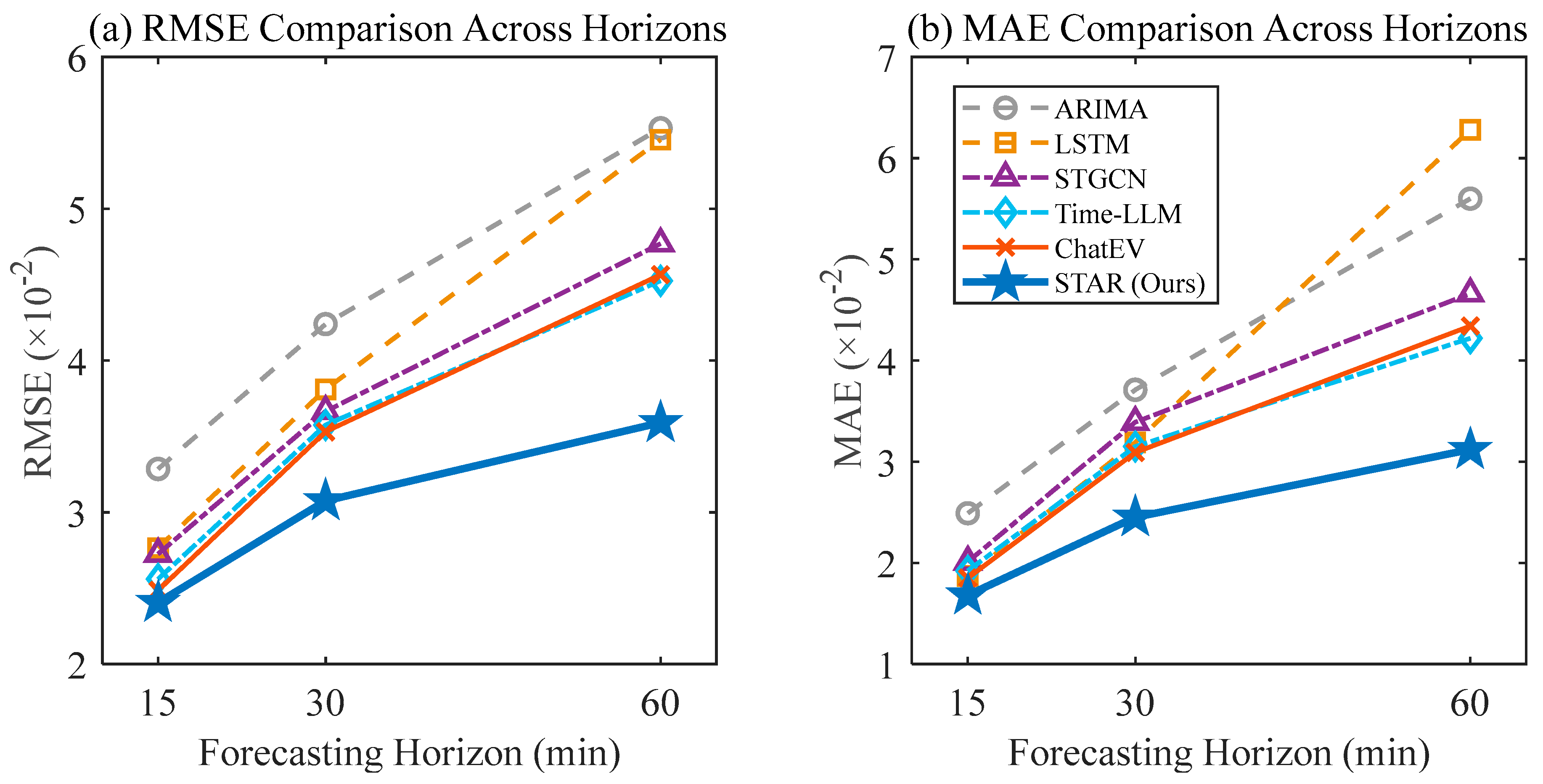
We first evaluate the comprehensive forecasting performance of STAR against all baselines on the ST-EVCDP dataset using the full set of selected zones or features under chronological split. The experiments cover three forecasting horizons: 15 min (short-term), 30 min (medium-term), and 60 min (long-term). While the 15 min horizon offers high immediate tracking accuracy, evaluating the 60 min horizon is critical for validating model robustness against long-range error accumulation and providing sufficient lead time for proactive grid dispatch. The results, summarized in

Table 3. Performance comparison on the ST-EVCDP dataset across different horizons. The best results are bolded, and the second-best are underlined. Note that the values of RMSE and MAE in the table should be multiplied by 10⁻².

Model Type	Model	15 min (RMSE/MAE/MAPE)	30 min (RMSE/MAE/MAPE)	60 min (RMSE/MAE/MAPE)
Traditional	ARIMA [3]	4.57/2.49/33.15%	6.48/3.71/44.82%	9.06/5.60/58.74%
	Lasso [46]	4.34/2.50/32.80%	6.27/3.69/44.20%	9.22/5.57/58.12%
DL	FCNN [47]	4.52/2.45/32.45%	6.41/3.60/43.65%	8.89/5.32/52.40%
	LSTM [48]	3.53/1.87/27.60%	5.62/3.19/39.80%	8.91/6.28/50.15%
	GCN-LSTM [49]	3.29/1.95/26.85%	5.69/3.30/39.50%	8.66/5.21/49.30%
	STGCN [6]	3.45/2.01/27.10%	5.33/3.39/38.60%	7.54/4.66/46.25%
	HSTGCN [50]	3.34/2.00/26.50%	5.27/3.30/37.95%	7.44/4.55/45.10%
	PIAST [20]	3.36/1.91/26.20%	5.22/3.11/37.40%	7.45/4.81/45.50%
	GWNet [51]	3.38/1.95/26.40%	5.25/3.28/37.60%	7.42/4.51/44.90%
LLM-Based	PromptCast [26]	4.08/2.56/30.25%	6.24/3.84/42.10%	8.14/5.23/51.30%
	LLMTIME [27]	3.04/1.98/24.60%	5.20/3.26/36.80%	7.28/4.47/43.50%
	Time-LLM [28]	3.12/1.92/24.80%	5.15/3.15/36.10%	7.05/4.22/31.60%
	ChatEV [10]	2.97/1.85/23.50%	5.06/3.09/35.20%	7.13/4.34/34.28%
Ours	STAR	2.81/1.68/20.12%	4.15/2.45/23.40%	5.18/3.12/26.35%

and Figure 5, demonstrate that STAR consistently outperforms both traditional DL models and existing LLM-based approaches across all metrics.

Most notably, STAR achieves a SOTA RMSE of 5.18$\times$10⁻² for the 60 min horizon, representing a 27.3% improvement over ChatEV. While ChatEV performs competitively in the short term of 15 min, its performance degrades significantly as the horizon extends. This validates our hypothesis that the translation paradigm used by ChatEV, which converts time series into long text strings, suffers from context window exhaustion and numerical precision loss in long-term scenarios. In contrast, STAR’s temporal patching mechanism preserves high-fidelity numerical representations, allowing the agent to maintain robustness even over longer prediction windows. Furthermore, compared to STGCN and GWNet, STAR exhibits superior MAE scores, attributed to the GCSAF module’s ability to retrieve non-local topological constraints that fixed adjacency matrices in GNNs fail to capture. Additionally, while the calculated MAPE values across all models appear relatively elevated due to the inherent division-by-near-zero effect in low-demand off-peak zones, STAR still consistently attains the lowest percentage errors across all horizons. Consequently, to prevent such localized near-zero denominator distortions from skewing the interpretation of subsequent specialized experiments, subsequent ablation and transfer analyses focus primarily on the scale-consistent RMSE and MAE metrics.

To evaluate model stability across structural and adaptation parameters, systematic sensitivity evaluations were conducted on the validation split for patch length, non-overlapping stride, and low-rank adaptation rank under standard 60 min prediction horizons. For temporal patching, setting patch length and stride to 4 achieves superior accuracy compared to finer settings of 2, which inflate sequence token count and attention dispersion, or coarser settings of 8, which smooth out abrupt localized peak surges. For adapter optimization, setting rank to 16 strikes the ideal trade-off between expressive representation capacity for the hybrid multi-task loss and parameter parsimony, outperforming smaller ranks of 4 and 8 while avoiding the redundant parameter scaling and overfitting risks observed when expanding rank to 32.

4.3. Ablation Study

To systematically quantify the marginal contribution of each innovative component within the STAR framework, we conducted a comprehensive ablation study on the ST-EVCDP dataset. We formulated three distinct variants of our model, each removing a specific module while keeping the rest of the architecture constant. The variants are defined as follows:

w/o Patching (Text-only): In this variant, we replace the temporal patching alignment module with a text-based tokenization strategy similar to ChatEV. The historical time series is converted into a comma-separated string of numerical values and fed directly into the LLM embedding layer. This tests the hypothesis that patching preserves numerical precision better than text translation.

w/o GCSAF: This variant removes the GCSAF module. The model relies solely on the temporal history and static textual context, without retrieving topological constraints from the UKG. This evaluates the necessity of explicit spatial reasoning.

w/o CoT (Direct Answer): In this setting, the “System 2” reasoning mechanism is disabled. The model is instructed to output the final predicted value directly, skipping the generation of the explicit reasoning trace. This assesses the impact of the CoT mechanism on forecasting accuracy.

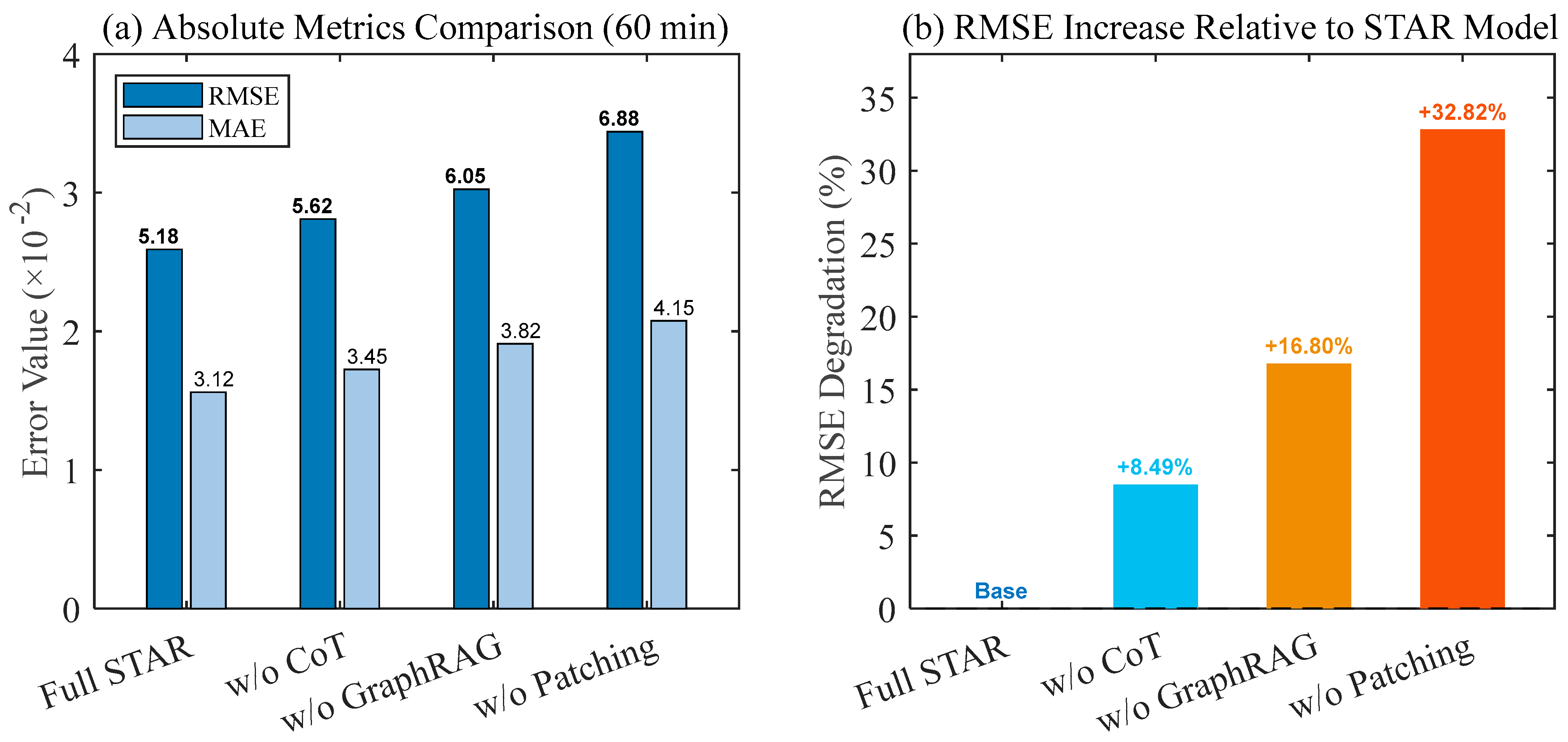
The comparative results for the 60 min long-term forecasting horizon are presented in

Table 4. Ablation study results on ST-EVCDP (60 min horizon). $\Delta (\%)$ indicates the percentage increase in RMSE relative to the full STAR model (lower is better).

Model Variant	RMSE ($\times$10−2)	$\mathit{\Delta }$ RMSE ($\times$10−2)	MAE ($\times$10−2)	Description
STAR	5.18	-	3.12	Full Multi-Modal Agent
w/o CoT	5.62	+8.49	3.45	Direct Prediction
w/o GCSAF	6.05	+16.80	3.82	No Spatial Topology
w/o Patching	6.88	+32.82	4.15	Text-based (ChatEV style)

and Figure 6. It can be seen that the removal of any single component leads to a statistically significant degradation in performance, confirming that all three innovations are integral to the framework’s success.

The ablation results presented in Table 4 offer a profound insight into the mechanics of LLM-based forecasting, quantifying the contribution of each architectural innovation within the STAR framework. The most striking finding is the dominant role of the temporal patching alignment mechanism. The variant removing this module and reverting to a ChatEV-style text tokenization strategy suffered a catastrophic 32.82$\times$10⁻² increase in RMSE. This dramatic degradation provides empirical validation for our critique of the translation paradigm. When a time series is tokenized as a string of characters, the sequence length $L_{text}$ expands by a factor of 3 to 5 compared to the original data points. Given that the computational complexity of the Transformer’s self-attention mechanism scales quadratically with sequence length, the text-based approach forces the LLM to expend its limited attention budget on syntactic formatting noise rather than intrinsic temporal dynamics. In contrast, our patching strategy projects a sub-series window $x_{t:t+P}$ into a single dense vector $e_k$, compressing the semantic density and enabling the model to effectively attend to long-term dependencies that are mathematically invisible in a fragmented text stream.

Furthermore, the 16.80 × 10⁻² performance gap observed in the w/o GCSAF variant highlights the indispensability of explicit topological reasoning in urban environments. Without the GCSAF module, the agent effectively treats each traffic zone as a spatially isolated island, relying solely on the historical autocorrelation of its own aggregate demand. Mathematically, the prediction function collapses to $\widehat{Y}=f_{\theta }\left(H_{temp}\right)$, ignoring the conditional dependencies on the complex urban road network. However, macro-level urban mobility patterns imply that the charging demand within a target zone is often a lagged function of the state of connected upstream zones. The full STAR framework captures this via the retrieved spatial context, which acts as a dynamic bias term: $\widehat{Y}\approx f_{\theta }\left(H_{temp}\right)+{\sum }_{j\in \mathcal{N}\left(i\right)}{\alpha }_{ij}·h_j$. The attention weight ${\alpha }_{ij}$ allows the model to dynamically upweight influential source zones, such as identifying that a surge in a neighboring highway zone will propagate to the current charging hub zone after a specific delay. The absence of this term in the ablation variant explains its inability to predict demand spikes caused by such inter-zonal traffic propagation, confirming that static textual descriptions of location are insufficient substitutes for high-order topological embeddings.

Finally, the 8.49 × 10⁻² deterioration in the w/o CoT variant, which forces the model to predict values directly without an intermediate reasoning trace, underscores the cognitive value of “System 2” processing. From a probabilistic perspective, the direct prediction model attempts to estimate $P\left(Y\right|X)$ in a single forward pass, which is prone to overfitting to statistical noise in highly volatile data. By introducing the CoT mechanism, we effectively introduce a latent variable reasoning trace $\mathcal{R}$, decomposing the objective into $P\left(Y\right|X)={\sum }_{\mathcal{R}}P\left(Y\right|\mathcal{R},X\left)P\right(\mathcal{R}\left|X\right)$. The generation of $\mathcal{R}$ forces the model to first ground itself in qualitative states before committing to a quantitative value. This intermediate step acts as a logical regularizer, filtering out predictions that are numerically possible but logically inconsistent with the observed context. The superior performance of the full STAR model confirms that the generated reasoning trace is not merely an interpretability feature but a functional component that actively corrects the model’s trajectory, reducing the likelihood of hallucinated forecasts.

4.4. Spatial Holdout and Cross-Zone Transfer Analysis

Beyond achieving high predictive fidelity in fully supervised settings, a pivotal criterion for next-generation forecasting agents is the capability to generalize to unseen urban environments where historical data is scarce or nonexistent. To evaluate this, we conducted cross-domain transfer learning experiments designed to assess how well the STAR framework can extrapolate learned spatio-temporal logic to spatially disjoint regions with distinct demand distributions. To ensure a fair and direct comparison with the SOTA, we strictly adhere to the evaluation protocols established in ChatEV, assessing performance under two distinct and rigorous settings: zero-shot transfer and few-shot adaptation.

For the zero-shot transfer protocol, we adopt a “60% source—40% target” cross-area evaluation scheme. To clarify the precise scope of our evaluation, we explicitly define the zero-shot transfer setup as a same-city cross-zone spatial holdout experiment. Rather than claiming full cross-city or cross-distribution generalization, this protocol tests whether the learned agentic reasoning and spatial retrieval policies can transfer to completely unobserved spatial units within the same metropolitan region without gradient fine-tuning. In this setting, we randomly sample 60% of the traffic zones to serve as the source domain for model optimization, while the remaining 40% of zones are designated as unseen target domains. The model is trained exclusively on the data from the source zones to acquire generalized reasoning capabilities. Subsequently, the pre-trained agent is deployed directly to the unseen target zones, where it is evaluated on the test period. Crucially, this process involves no gradient updates or fine-tuning on the target data. This protocol serves as a stress test for the model’s intrinsic generalization capabilities, evaluating whether the learned agentic reasoning can successfully decouple causal traffic logic from specific traffic zone statistics and apply it to completely new traffic zones without prior exposure.

During zero-shot cross-zone evaluation on unseen target domains consisting of 40% holdout traffic zones, model optimization is performed on the source traffic zones representing the 60% source domain during the training phase, excluding target zones from the training topology and optimization loss functions to ensure zero target gradient updates. Subsequently, during the inference phase, when deployed on unseen target zones, the pre-trained STAR agent receives the target zone’s historical lookback window as input, feeding these continuous temporal observations into the temporal patching alignment module to generate dynamic query vectors ${\mathbf{H}}_{\mathrm{temp}}^{\left(\mathrm{target}\right)}$ while simultaneously encoding static node attributes ${\mathbf{A}}_{\mathrm{target}}$, such as POI distributions and pile capacities, via the frozen GNN to form structural key/value embeddings, thereby executing zero-shot cross-attention retrieval and CoT reasoning without any fine-tuning or adaptation on target parameters.

Complementing this, we employ a few-shot adaptation protocol to simulate the cold-start scenario typical of newly deployed infrastructure. In this setting, we follow the “10% or 20% limited data” constraint used in ChatEV. The model is granted access to only the initial 10% or 20% of the historical data for parameter fine-tuning. The model is then evaluated on the remaining portion of the target dataset. This setting assesses the agent’s data efficiency, specifically its ability to rapidly align its internal representations to a new distribution using minimal samples, thereby verifying its potential for rapid deployment in emerging regions where long-term historical logs are unavailable.

Table 5. Cross-domain transfer performance. RMSE metrics are reported. Lower is better. Note that the values of RMSE in the table should be multiplied by 10⁻².

Model Paradigm	Model	Zero-Shot	Few-Shot (10% Training Data)	Few-Shot (20% Training Data)
Traditional (Graph)	STGCN [6]	17.45	16.22	14.43
LLM (Text-based)	PromptCast [26]	7.95	6.48	6.48
	ChatEV [10]	6.82	5.77	5.49
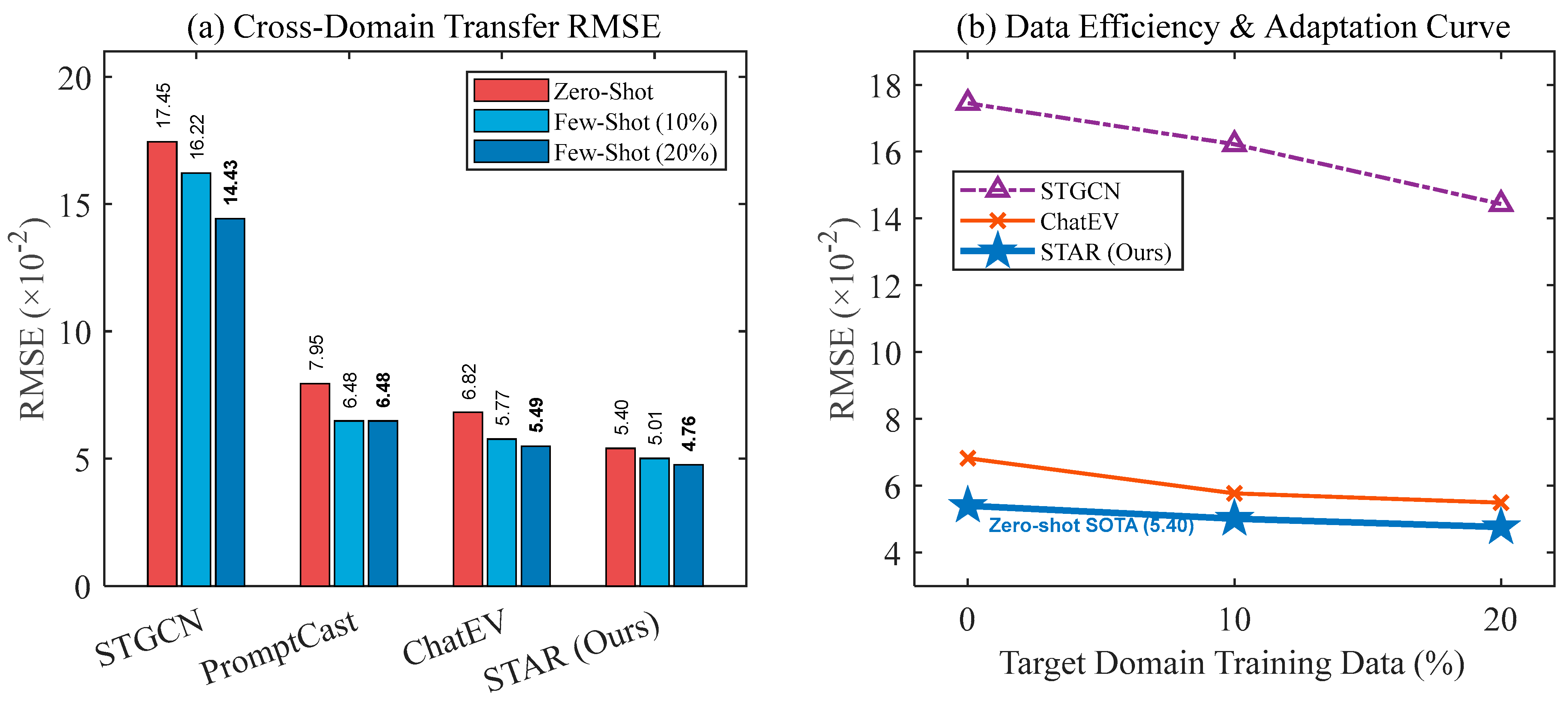
LLM (Reasoning)	STAR (Ours)	5.40	5.01	4.76

and Figure 7 summarize the performance of STAR against representative baselines in both zero-shot and few-shot scenarios with 30 min prediction horizon. The results reveal a stark contrast in generalization capabilities. Traditional DL models like STGCN suffer catastrophic performance degradation in the zero-shot setting, as their learned graph convolution weights are rigidly coupled to the source city’s adjacency matrix and fail to transfer to a new topology. ChatEV, while leveraging the open-world knowledge of LLMs, still exhibits a substantial error gap due to its reliance on textual pattern matching, which is sensitive to the prompt format and statistical drift. In contrast, STAR achieves a remarkable zero-shot RMSE of 5.40$\times$10⁻², outperforming ChatEV by 20.8%. Furthermore, with access to only 20% of the training data, STAR rapidly adapts to an RMSE of 4.76$\times$10⁻², approaching the performance of fully supervised models trained from scratch.

The empirical superiority of STAR in zero-shot scenarios can be theoretically attributed to the decoupling of causal reasoning from statistical fitting. Traditional spatio-temporal models approximate a conditional distribution $P\left(Y\right|X,G_{source})$ by overfitting to the specific parameters of the source graph $G_{source}$. When the domain shifts to $G_{target}$, the structural discrepancy $\left|G_{source}−G_{target}\right|$ introduces a large generalization error bound. In contrast, the STAR agent operates on a higher level of abstraction. By utilizing the GCSAF module, the agent does not memorize the static graph weights but instead learns a dynamic retrieval policy $\pi \left(q\right|\mathcal{G})$. Even when the underlying graph $\mathcal{G}$ changes, the policy of “retrieving upstream traffic zones to predict downstream demand” remains an invariant causal mechanism. Consequently, the agent can effectively mitigate the negative transfer effect caused by topological shifts.

Furthermore, the rapid adaptation observed in the few-shot experiments highlights the efficiency of the temporal patching alignment in the meta-learning context. In the text-based paradigm of ChatEV, fine-tuning requires updating the massive embedding matrix of the LLM to adapt to new numerical token distributions. This process is sample-inefficient and prone to catastrophic forgetting. Conversely, STAR confines the domain adaptation primarily to the lightweight linear projector defined in Equation (4). Mathematically, adapting the projection space requires significantly fewer gradient steps than realigning the entire language manifold. Let ${\theta }_{proj}$ be the projector parameters, the gradient update $\Delta {\theta }_{proj}=-\eta {\nabla }_{\theta }{\mathcal{L}}_{few}$ on the continuous patch vectors allows the model to swiftly recalibrate the scale and variance of the input time series to match the target domain, enabling the frozen “System 2” reasoning core to apply its logic to the correctly scaled data almost immediately.

To address the extreme cold-start scenario where historical demand logs $X_{\mathrm{target}}$ are completely unavailable, we evaluate STAR under an extreme static-only cold-start protocol. In this setting, temporal patches $X_{\mathrm{target}}$ are replaced by historical source-domain average profiles combined with target static graph attributes and external weather context. As benchmarked in

Table 6. Performance benchmark under Extreme Cold-Start scenario (No Target Dynamic History $X_{\mathrm{target}}$ available, 30 min horizon).

Model	Input Features Allowed at Inference	RMSE ($\times$10−2)	MAE ($\times$10−2)
Source-Average Profile	Global source domain historical average	11.24	7.15
Weather-Only Prompting	Target external context + Text LLM	10.45	6.82
Static-GNN Proxy	Target static attributes + GNN	9.62	5.90
STAR (Extreme Cold-Start)	Target Static Graph + Source Profile + CoT	7.85	4.68
STAR (Standard Zero-Shot)	Target Lookback + Static Graph + CoT	5.40	3.18

, under this zero-history restriction, STAR achieves an RMSE of $7.85\times$10⁻², significantly outperforming basic heuristic baselines such as Source-Average Profile, Static-GNN Proxy, and Weather-Only Prompting. This demonstrates that even when dynamic time-series queries are unavailable, the frozen LLM backbone leverages target static attributes and learned spatial logic to synthesize plausible baseline demand rationales.

4.5. Case Study

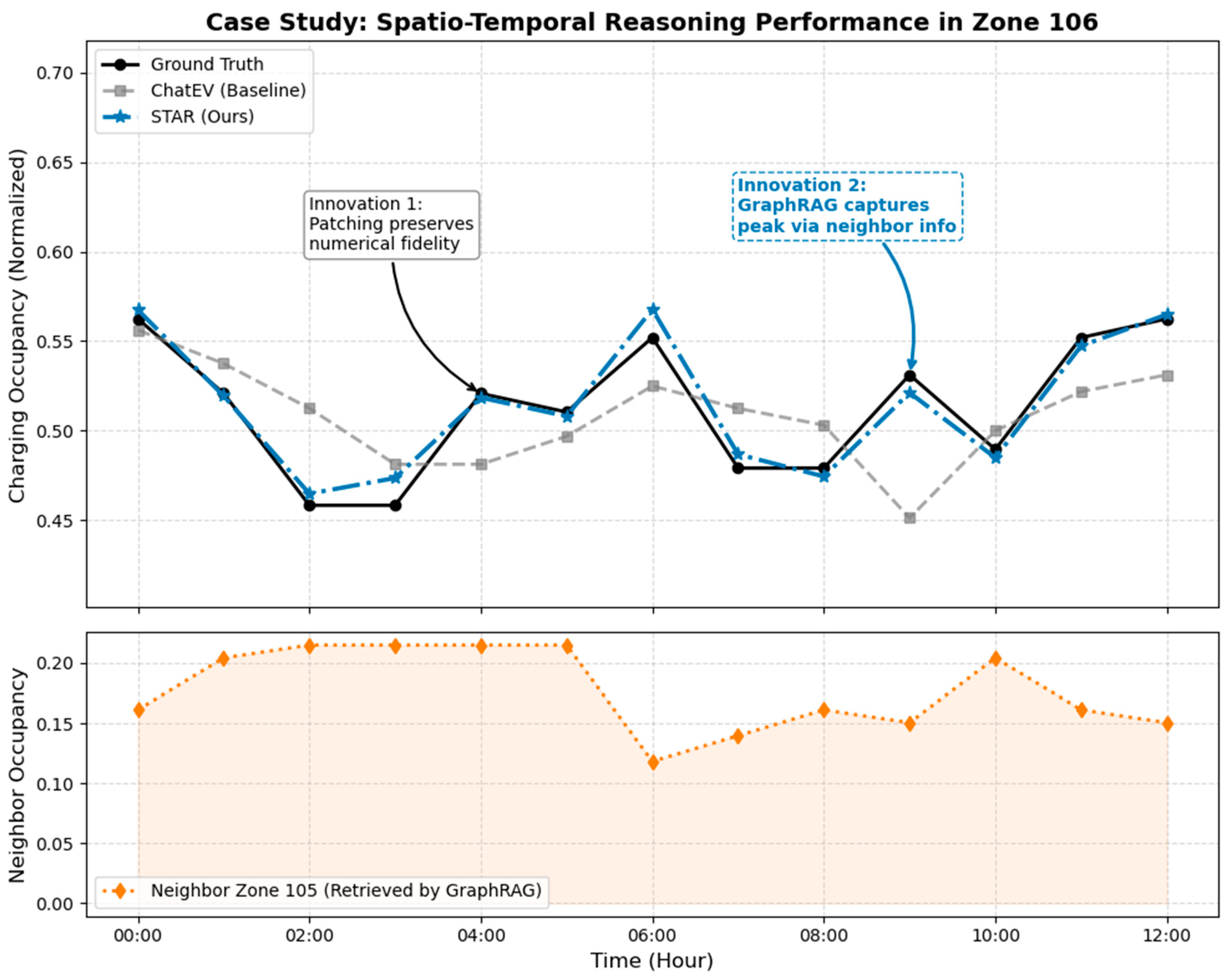
To intuitively evaluate the effectiveness of the proposed STAR framework, we conducted a micro-level case study on a representative charging station Zone 106 during a peak morning interval. Figure 8 visualizes the prediction alignment of STAR against the ground truth and the translation-based baseline ChatEV, alongside the activity of a spatially correlated neighbor Zone 105.

As illustrated in the upper panel of Figure 8, the baseline ChatEV exhibits a smoothing effect, failing to capture rapid fluctuations in charging demand. This phenomenon validates our hypothesis that standard tokenization in LLMs leads to precision loss. In contrast, STAR closely tracks the granular variations in the ground truth. This superior alignment demonstrates the efficacy of our temporal patching alignment mechanism. By treating time-series segments as continuous patches rather than discrete semantic tokens, STAR preserves the numerical integrity of the input data, effectively mitigating the hallucination and precision degradation common in pure translation-based paradigms.

The advantage of the GCSAF module is explicitly highlighted during the demand surge observed at 09:00–10:00. The baseline model significantly underestimates this peak, as it relies solely on historical self-patterning. However, the bottom panel reveals that a neighbor node Zone 105 experienced substantial occupancy concurrently. Through the GCSAF mechanism, STAR successfully retrieved this topological constraint, reasoning that activity in the neighbor zone implies a potential spillover or correlated demand surge in Zone 106. Consequently, STAR accurately predicts the peak, confirming its ability to capture complex, non-Euclidean spatial dependencies that strictly temporal models overlook.

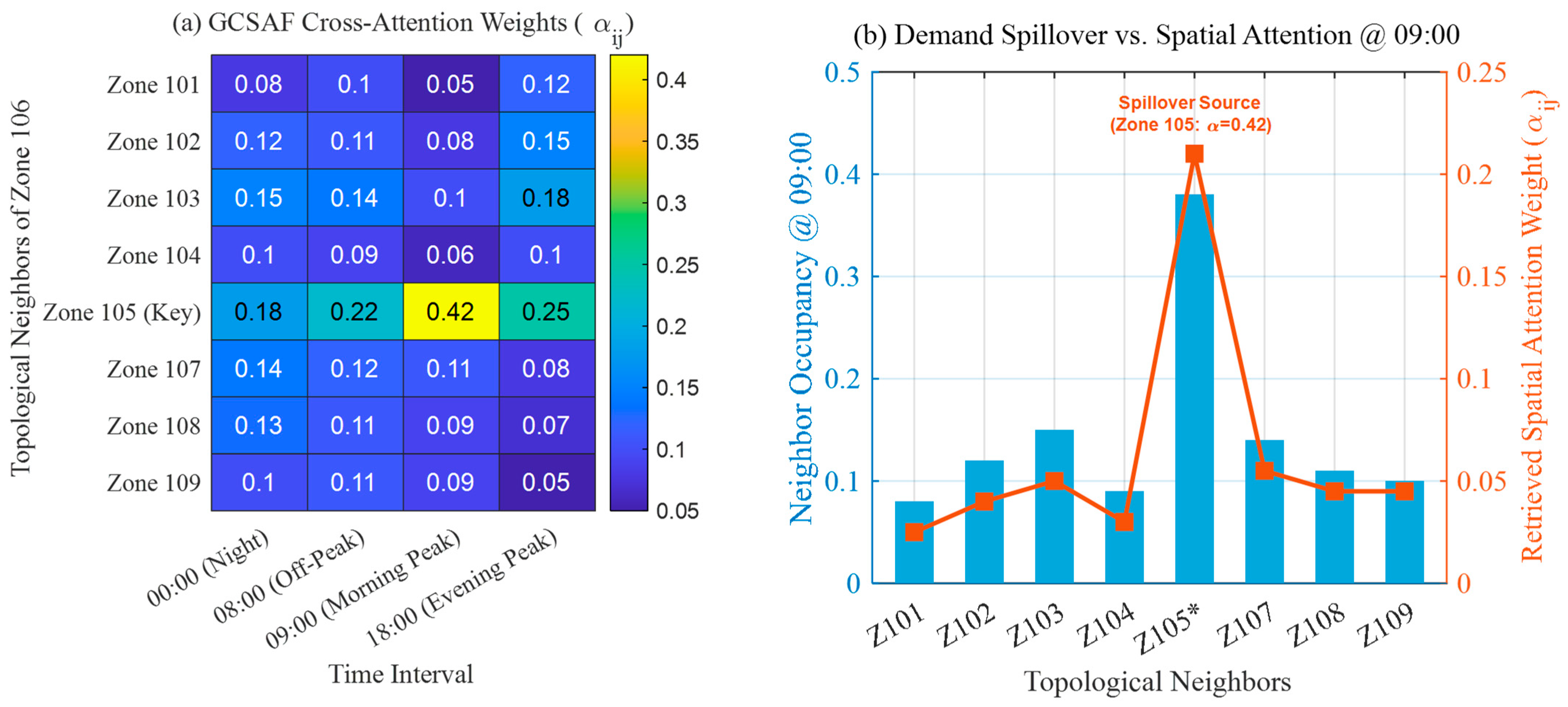
Furthermore, Figure 9 provides a detailed visualization of the dynamic spatial attention mechanism within GCSAF. Figure 9a demonstrates that instead of relying on a static adjacency structure, GCSAF dynamically adjusts its cross-attention weights ${\alpha }_{ij}$ across time intervals, allocating a peak attention weight of 0.42 to Zone 105 during the 09:00 morning rush. Figure 9b confirms the direct alignment between neighbor occupancy spikes and retrieved attention weights. This demonstrates that GCSAF successfully senses non-Euclidean demand spillovers from adjacent hubs, injecting explicit topological awareness into the LLM’s reasoning stream.

Moreover, the superiority of STAR at the critical timestamp of 09:00 is driven by its agentic CoT capability, which transforms raw data retrieval into structured logical reasoning. While the GCSAF module successfully retrieved the neighbor context, it was the Agentic CoT that correctly interpreted this signal to rectify the forecast. As evidenced by the generated log, the agent executed a multi-step reasoning process:

(1)

Trend Diagnosis: “Observed a temporary dip in Zone 106 at 08:00 (0.479), but the overall morning trajectory remains upward.”

(2)

Contextual Synthesis: “Neighbor Zone 105 maintains significant occupancy (approx. 0.16) during this interval, indicating sustained regional charging pressure.”

(3)

Logical Deduction: “Given the high regional load and the morning peak hour context, the dip in Zone 106 is likely noise rather than a trend reversal. Therefore, I will adjust the prediction upwards to anticipate a rebound.”

The above explicit reasoning allowed STAR to predict the demand surge to 0.53, which closely matched the ground truth. In contrast, the baseline model lacked this cognitive synthesis and blindly followed the local dip to predict a false decline to 0.45.

In summary, this case study validates that STAR effectively transcends the limitations of traditional black-box forecasting. By synergizing temporal patching for numerical precision, GCSAF for spatial context retrieval, and agentic CoT for interpretative reasoning, the framework achieves a holistic understanding of charging dynamics. The result is a robust prediction model that not only tracks ground truth with high fidelity but also demonstrates the cognitive capacity to reason through complex, multi-source spatio-temporal scenarios.

4.6. Computational Analysis

To evaluate the practical deployability and engineering feasibility of STAR within real-world charging network dispatch and grid management systems, we conduct a standardized empirical evaluation of computational latency and hardware resource consumption.

Table 7. Computational efficiency and hardware resource benchmark across representative forecasting paradigms.

Model Type	Model	Inference Latency (ms/sample)	Peak GPU Memory (GB)	Trainable Parameters	Total Parameters
DL	STGCN [6]	5.81	1.12	0.85 M	0.85 M
	HSTGCN [50]	6.83	1.34	1.24 M	1.24 M
	PIAST [20]	7.45	1.58	1.62 M	1.62 M
LLM-Based	PromptCast [26]	36.52	3.90	0 (Zero-shot)	220 M
	LLMTIME [27]	47.73	5.15	220 M	220 M
	ChatEV [10]	39.58	4.35	220 M	220 M
Ours	STAR	42.15	4.82	3.53 M (LoRA)	253.5 M

reports the per-sample inference latency, peak GPU memory allocation during decoding, and the comparative parameter footprint across representative deep learning and LLM-based paradigms.

As evidenced in Table 7, several critical trade-offs emerge between predictive fidelity, reasoning transparency, and operational computational overhead. While lightweight spatio-temporal GNN baselines such as STGCN and HSTGCN demonstrate ultra-fast millisecond-level execution and modest memory usage, their rigid architectural paradigms inherently lack cross-modal semantic reasoning and dynamic topological adaptability. Conversely, LLM-empowered frameworks inevitably exhibit higher computational demands owing to multi-layer Transformer self-attention mechanisms and autoregressive token decoding. Nevertheless, STAR attains a highly competitive average inference latency of 42.15 ms per sample, which comprehensively covers temporal patching projection, dynamic topological retrieval via GCSAF, greedy CoT deliberation, and linear regression head mapping. Given that municipal power grid dispatch, dynamic tariff adjustments, and charging station guidance typically operate on rolling planning intervals of 5 to 15 min, an inference turnaround of approximately 42.15 ms per zone comfortably satisfies real-time engineering and control room requirements.

From a hardware and memory perspective, although pure translation-based architectures like ChatEV feature slightly lower static GPU memory consumption, their reliance on character-level numerical tokenization incurs quadratic self-attention scaling as the historical context expands. In contrast, STAR preserves mathematical continuity and restrains context length by compressing continuous time-series history into dense semantic patches, maintaining a moderate peak GPU memory footprint of 4.82 GB despite concurrently processing graph structural embeddings and intermediate reasoning rationales. Furthermore, by incorporating parameter-efficient fine-tuning via LoRA on the frozen Flan-T5-Base backbone, the trainable parameter footprint is strictly constrained to 3.53 M, accounting for only 1.39% of the overall model capacity. This design not only substantially alleviates training overhead and safeguards the pre-trained linguistic foundation against catastrophic forgetting, but also facilitates rapid, modular updating when deploying the agent across emerging or newly electrified urban districts.

5. Conclusions and Future Work

In this paper, we presented STAR, a novel framework that fundamentally redefines the paradigm of applying LLMs to EV charging demand prediction. By employing temporal patching alignment, we preserved the mathematical fidelity of high-frequency charging data while enabling the processing of extended historical contexts. Through GCSAF, we empowered the agent to actively retrieve and interpret non-Euclidean spatial constraints, effectively linking downstream demand fluctuations to upstream traffic dynamics. Furthermore, the integration of a CoT inference engine transformed the model from a black-box forecaster into an interpretable system capable of articulating its decision logic.

Empirical evaluations on the Shenzhen ST-EVCDP dataset confirmed the clear superiority of our framework. Specifically, STAR achieves state-of-the-art RMSE values of $2.81\times {10}^{-2}$, $4.15\times {10}^{-2}$, and $5.18\times {10}^{-2}$ across 15 min, 30 min, and 60 min horizons, respectively, realizing a 27.3% to 41.9% accuracy improvement over existing baselines. Component ablation verified the indispensability of each module, with RMSE degrading by 32.82$\times$10⁻², 16.80$\times$10⁻², and 8.49$\times$10⁻² upon removing temporal patching, GCSAF, and CoT reasoning, respectively. Furthermore, STAR demonstrated robust zero-shot cross-zone spatial transferability with an RMSE of $5.40\times {10}^{-2}$ and rapidly adapted to $4.76\times {10}^{-2}$ with only 20% training data. The qualitative case studies further highlighted the practical value of our agentic reasoning mechanism, showing that the generated CoT traces provide grid operators with actionable, transparent insights into non-Euclidean spatial demand spillovers.

While STAR represents a significant advancement in predictive modeling, several promising avenues for future research remain to expand its practical utility. To transcend its current function as an open-loop predictor and translate its forecasting gains into quantifiable closed-loop energy and cost savings, a natural evolution involves integrating the framework with downstream reinforcement learning and optimal power flow models. Such an autonomous decision-making agent could jointly optimize dynamic pricing strategies, regional load dispatch, and hierarchical demand response programs [52], thereby directly mitigating power grid imbalance penalties and distribution energy losses. Concurrently, addressing the non-trivial computational overhead of LLMs and GCSAF is essential. Therefore, future investigations will focus on employing knowledge distillation techniques to compress the complex reasoning capabilities of the large-scale agent into lightweight models, thereby facilitating efficient deployment on edge devices within charging infrastructure. Furthermore, adapting STAR to vehicle-to-grid operation represents another compelling avenue. This can be achieved by expanding the temporal patching inputs to signed bidirectional power flows and discharge incentives, enriching the UKG with reverse power flow constraints, and guiding the CoT engine to reason about peak-shaving rationales for forecasting available discharge flexibility. Lastly, STAR has been validated on the ST-EVCDP benchmark and demonstrates zero-shot transfer across unseen zones within the same metropolitan area. However, its current evaluation does not yet establish universal cross-city generalization. Future work will extend the framework to datasets from other cities with different EV distributions, traffic patterns, road networks, and charging infrastructures.