Article

A Grid-Forming Control Strategy Based on a Hybrid Approach Combining a Physical Model and LSTM for Photovoltaic and Energy Storage Systems


1
School of Electrical Engineering, Hebei University of Science and Technology, Shijiazhuang 050018, China
2
Hebei Province Construction & Investment Group Co., Ltd., Shijiazhuang 050051, China
3
Hebei Suntien New Energy Technology Co., Ltd., Zhangjiakou 075131, China
4
Suntien Green Energy Co., Ltd., Shijiazhuang 050051, China
*
Author to whom correspondence should be addressed.
Electronics 2026, 15(17), 3782; https://doi.org/10.3390/electronics15173782
Submission received: 9 July 2026 / Revised: 18 August 2026 / Accepted: 20 August 2026 / Published: 24 August 2026
(This article belongs to the Section Systems & Control Engineering)

Abstract

Traditional grid-forming converter (GFC) control faces fundamental challenges in maintaining DC bus stability during rapid power transients, primarily due to the limited dynamic response capability of source-side energy storage devices. To address this, this paper proposes a hybrid control strategy integrating long short-term memory (LSTM) networks with a joint GFC and storage converter (SC) control scheme. The LSTM detects short-term voltage trends from historical DC bus data to generate a feedforward compensation signal, while the joint SC-GFC control dynamically incorporates the GFC’s inertial power demand into the SC’s power reference. Hardware-in-the-loop experiments show that, compared to traditional independent control under the same step transient conditions, the proposed method can reduce power overshoot by approximately 79.2%. The LSTM-enhanced joint control maintains stable power flow and significantly suppresses low-frequency oscillations, validating the necessity of data-driven trend prediction for achieving superior inertial support in practical constrained environments. This work provides a communication-free, practical solution for enhancing GFC performance.

1. Introduction

With the rapid development of renewable energy, distributed energy sources have gradually become an important part of the power system [1,2,3]. In this context, the grid-forming converter (GFC) has emerged as a crucial device for maintaining grid stability and is widely adopted in microgrids and distributed generation systems [4,5]. However, traditional GFC control strategies, which often rely on fixed parameters, can become mismatched under real-world conditions such as source-side storage performance degradation and dynamic load variations. Such a control mismatch can consequently lead to degraded dynamic performance or even system instability.
In recent years, scholars at home and abroad have carried out extensive research on the dynamic characteristics of the grid-forming control. Ref. [6] proposed the concept of damped area approximation to evaluate the effect of damping on the attraction domain in a quantitative and intuitive way. Ref. [7] solved the problem of power angle instability in shunt inverters by introducing additional adaptive control loops to reduce the power control points of the grid-forming control. Ref. [8] analyzed the system oscillation frequency and its influence range by using the loop impedance matrix of a multi-GFC system and proposed a modal evaluation method. Ref. [9] pointed out that the strong nonlinearity of GFC increases the complexity of transient stability analysis, and proposed an equal proportional area criterion based on the flexible control of inertia coefficients. Ref. [10] studied the coupling mechanism between voltage and frequency of GFC in depth, and proposed a unified stability analysis model for voltage, frequency and their coupling. However, the above methods focus on the analysis of GFC operation characteristics and do not consider the interaction between new energy sources, energy storage and power grids. The energy storage devices underpinning GFC operation must therefore possess both fast response capabilities and high reliability. Consequently, researchers have focused on enhancing the GFC control strategies to improve the synchronization stability. Ref. [11] proposes to improve the system robustness based on the interconnection damping distribution passive control. Ref. [12] proposed to implement damping improvement in transient electromagnetic power compensation and transient damped power compensation based on virtual synchronization strategy. Ref. [13] developed an overshoot compensator to achieve the reshaping of synchronization phase for grid-forming grid-connected control and thus improve the transient performance.
However, the aforementioned methods primarily focus on improving the internal algorithms of the GFC and are typically validated under idealized assumptions—namely, that the DC-side power source is an ideal voltage source or a battery with infinite capacity. Such assumptions are difficult to satisfy in real-world systems because source-side energy storage devices have limited dynamic response capabilities. In fact, while the GFC control algorithm itself can provide virtual inertia, the energy for its inertial power output ultimately originates from the DC side. When the source-side energy storage devices are unable to replenish energy in a timely manner due to capacity limitations, performance degradation, or slow control response, the GFC’s inertial support capability is significantly compromised, potentially leading to DC bus voltage collapse and system instability.
In addition, data-driven methods based on artificial intelligence offer new perspectives for control optimization in distribution networks. Refs. [14,15] proposed a data-driven approach to estimate the attractor domain of power systems incorporating GFCs while developing novel control strategies. Ref. [16] introduced a model-based reinforcement learning algorithm capable of approximating the dynamic process of GFCs through dynamic programming. Ref. [17] proposes a data-driven GFC pre-synchronization method. Beyond converter control, recent work has also demonstrated the effectiveness of deep recurrent networks for short-term forecasting of residential net-load and EV charging, highlighting the potential of data-driven time-series modeling in renewable-integrated systems [18]. When the inertial power demand of the GFC exceeds the storage converter’s (SC) ability to respond, the DC bus voltage becomes unstable, leading to system oscillations or even collapse. Therefore, the core challenge shifts from merely designing a robust GFC to managing the dynamic power balance at the DC link itself. Some data-driven approaches [14,15,16,17,18] have been explored, but they often depend on external communication networks, introducing latency and reliability concerns. Therefore, the core challenge has shifted from simply designing a robust GFC to managing the dynamic power balance of the DC bus itself. Conventional SC control operates in a passive response mode—the SC only begins to act when the DC bus voltage has already deviated from the reference value. This inevitably introduces a delay that cannot keep pace with the rapid inertial demands of the GFC.
To address these challenges, this paper proposes a hybrid drive strategy combining proactive prediction and cooperative control. Rather than using Long Short-Term Memory (LSTM) networks to predict external disturbances, we leverage their time-series modeling capabilities to detect impending power imbalance trends from historical fluctuations in the DC bus voltage, thereby providing a feedforward compensation signal to the SC. Based on this, a joint control architecture for the SC and GFC is designed, incorporating the GFC’s inertial power demand as an input to the SC’s outer-loop power control to achieve dynamic coordination between the two. This approach requires no external communication and effectively enhances the system’s dynamic stability in scenarios with limited energy storage capacity. Unlike existing methods, this work uniquely combines (i) a joint SC-GFC control architecture that feeds the GFC’s inertial power demand back to the SC, and (ii) a communication-free LSTM feedforward path that anticipates voltage trends. The novelty lies in the synergistic integration of physical feedback control and data-driven trend prediction within a single closed-loop framework. A comparison table is shown in Table 1.
The specific contributions of this paper are:
  • A joint SC-GFC control architecture that feeds the GFC’s inertial power demand to the SC power loop.
  • An LSTM-based feedforward path that extracts voltage trends from historical Udc data.
  • A hybrid physical-data-driven framework that weights and fuses feedback and feedforward signals.
The sections of this paper are organized as follows: Section 2 introduces the system structure of this paper as well as the basic control method. Section 3 introduces the modeling of energy storage devices and the equivalent modeling of PV devices. Section 4 describes the LSTM trend-sensing method and the design of the SC-GFC joint control system. Section 5 is the evaluation of the rationality of the methodology and modeling described in this paper through hardware-in-the-loop validation. Section 6 is the conclusion of this paper.

2. System Configuration

2.1. Power Model of GFM-ESS

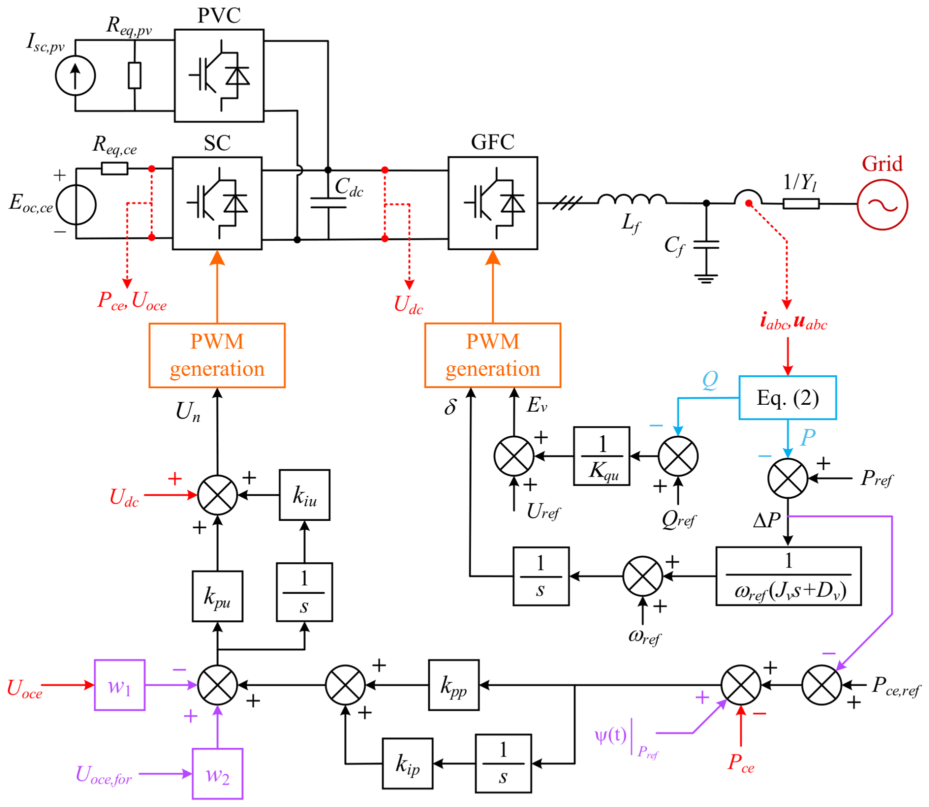
Figure 1 illustrates the detailed configuration of the GFC-based grid-connected system. At the point of common coupling (PCC), the three-phase currents and voltages are denoted as iabc and uabc, respectively. The GFC supplies active power Pv and reactive power Qv to the AC side, with its internal electromotive force Ev and the PCC voltage Ep determining the power exchange. The phase angles of the GFC and the grid are represented by d and q, while Lf and Cf denote the filter inductance and capacitance. It is worth noting that the LC filter is damped by a series resistor Rf to suppress high-frequency resonance [19]. Rf is not shown in Figure 1 because the internal resistance of Lf acts as part of the damping resistance, and together with the additional series resistor, they form Rf.
For instantaneous power calculation, we adopt the Clarke-transformation-based approach proposed in [20]. This method circumvents the synchronization errors that typically arise when computing power in the dq reference frame under unbalanced or distorted grid conditions.
P v = E v E p Y l sin δ θ arg Y g Re Y l E p 2 Q v = E v E p Y l cos δ θ + arg Y g Im Y l E p 2
Based on the power calculation results, a first-order low-pass filter with cutoff frequency ωf is introduced to smooth the measured power, yielding:
P v = ω f s + ω f i α β T u α β Q v = ω f s + ω f i α β T 0 1 1 0 u α β
where: iαβ = [iα, iβ]T and uαβ = [uα, uβ]T are the Clarke transform results of sampling three-phase current and three-phase voltage, respectively.

2.2. Basic Grid-Forming Control

The grid-forming converter enables direct regulation of system frequency and voltage through built-in virtual inertia and damping characteristics. Its core lies in achieving dynamic characteristics similar to those of a synchronous generator through active and reactive power control loop design. Currently, common GFC control strategies include droop control, virtual synchronous generator (VSG), and virtual oscillator etc. In this work, VSG is used as the control strategy of GFC.
The VSG control strategy emulates the electromechanical behavior of a conventional synchronous generator by replicating its stator-voltage and rotor-swing dynamics [21]. The evolution of the power angle is governed by the well-established second-order swing equation, which captures the interaction between the mechanical input and the electrical output of the virtual machine. This equation is a set of second-order nonlinear differential equations which describes the relationship between the mechanical and electromagnetic power of the moving rotor. Based on this equation the process of rotor motion to generate the power angle can be described as:
d δ d t = ω v J v d ω v d t = P r e f P v ω r e f D v ω v ω r e f
In the above equations, ωref denotes the nominal angular frequency, while ωv represents the instantaneous frequency of the VSG. The term Pref corresponds to the mechanical driving power, which in this context serves as the active power setpoint. The parameters Jv and Dv are the virtual inertia and damping coefficients, respectively, and the angles d and q track the real-time phase of the GFC relative to the grid.
The excitation voltage of the VSG is synthesized from a nominal voltage reference and the reactive-power error, following a droop-type characteristic. This formulation mirrors the conventional reactive-power/voltage droop control used in parallel-operated converters. Defining the droop coefficient Kqu, the induced electromotive force Ev of the VSG is expressed as:
E v = U r e f + 1 K q u Q r e f Q v
where Uref is the voltage reference value; Qref is the reactive power reference value.

2.3. Source Measurement Storage Converter Control

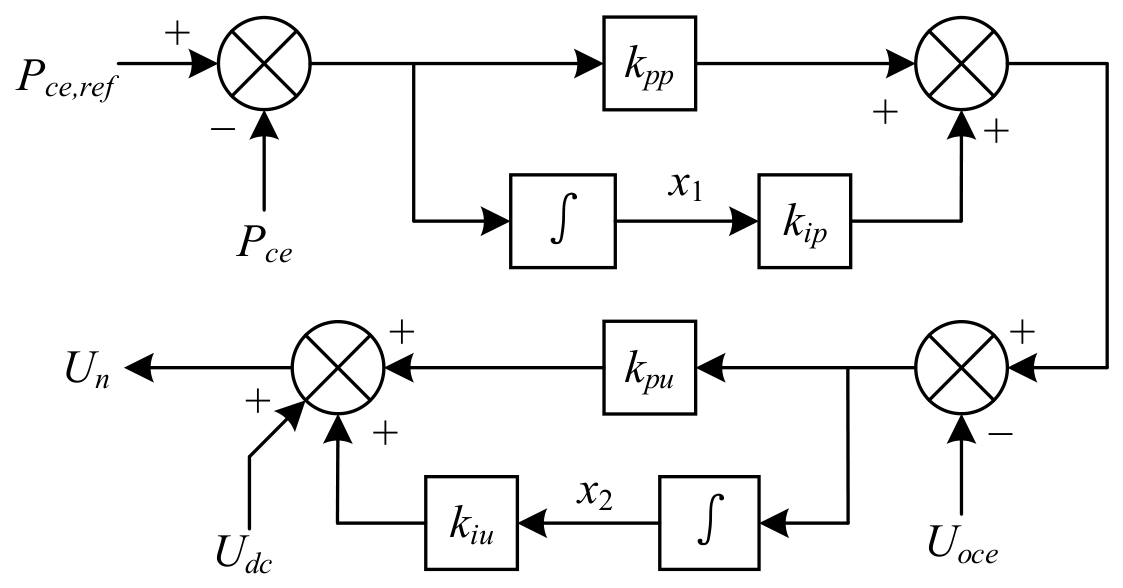
The SC is a bidirectional DC-DC power stage that must deliver rapid power response to support the GFC during transients. To achieve this, a two-level cascade control structure is adopted, comprising an outer power-regulation loop and an inner voltage-regulation loop, as depicted in Figure 2. This cascade arrangement enables independent tuning of dynamic tracking and steady-state accuracy—the inner loop handles fast disturbance rejection, while the outer loop governs the power-scheduling performance.
The inner loop employs a high-bandwidth PI compensator to regulate the converter output current/voltage in real time, ensuring that the actual power delivery closely follows the reference command from the outer loop. The outer loop, operating at a slower time scale, adjusts the power reference based on the system-level requirements, such as the GFC’s inertial power demand or the dispatched charging/discharging profile. This hierarchical design ensures robust performance under a wide range of operating scenarios.
With reference to the control block diagram in Figure 2, the state variables of the system are defined as x = [x1, x2]T. The input vector u = [Pce,ref, Pce, Uoce, Udc]T includes the power setpoint, the measured output power, the battery terminal voltage, and the DC bus voltage. The output of the controller is the converter modulation index y = Un. The resulting state-space description is given by (5) and (6).
x ˙ 1 = P c e , r e f P c e x ˙ 2 = k i p x 1 + k p p P c e , r e f P c e U o c e
y = k p u k i p x 1 + k i u x 2 + k p u k p p P c e , r e f P c e k p u U o c e
where Pce,ref represents the dispatch power of the energy storage device, which is positive at the time of discharge; Pce represents the output power of the energy storage device; Uoce is the terminal voltage of the energy storage device; and Udc represents the bus voltage. In addition, the following definitions are made for the control parameters: kpp and kip are the proportional and integral parameters for the power outer loop control; kpu and kiu are the proportional and integral parameters for the voltage internalization control.
It should be noted that this paper focuses on the upper-level coordinated control algorithms for the SC and GFC, specifically on how to generate reference values such as Pce,ref, and Pref, rather than on the detailed protection design of the lower-level converters. Therefore, a classic PI structure is adopted in the control loop, with its parameters tuned according to the system’s dynamic response requirements. In practical engineering applications, protection modules such as current limiting and fault ride-through can be added on top of this foundation without affecting the effectiveness of the high-level control strategy proposed in this paper.

2.4. Photovoltaic Converter Control

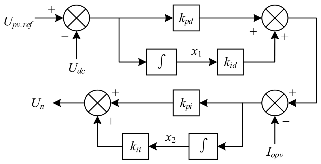
The PV-side converter (PVC) also employs a DC-DC boost stage with a cascade control configuration, as shown in Figure 3. Its primary function is to regulate the DC bus voltage while extracting maximum or dispatchable power from the PV array. The control architecture mirrors that of the SC, with a voltage outer loop and a current inner loop. Consequently, the state equations of the PVC controller share the same structure as (5) and (6), differing only in the specific gain values used for the PV-side dynamics.

3. Modeling of Energy Storage and PV Devices

3.1. Equivalent Model of the Energy Storage Device

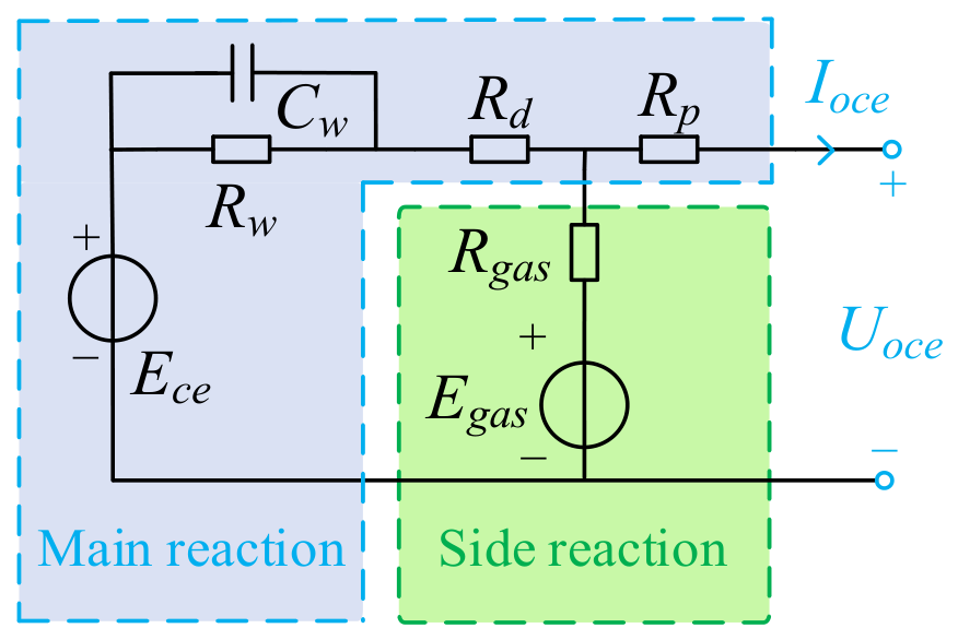
The dynamic behavior of the GFC is closely tied to the characteristics of its DC-side energy source. Inadequate storage capacity or age-induced performance deterioration can significantly degrade the overall system response. To accurately represent the battery dynamics in simulation and hardware testing, we adopt a third-order electrochemical equivalent circuit that captures both the primary and secondary reactions during charge/discharge cycles.
For a lithium-ion cell, the primary electrochemical process involves the reversible redox reaction of LiCoO2 during discharge and its reverse during charging. Alongside this main reaction, parasitic side reactions—such as gas evolution with the electrolyte solvent—also occur and are particularly pronounced under overcharge conditions. Following the framework originally developed for lead-acid batteries in [22], we construct a third-order dynamic equivalent circuit that accounts for both the main and side reactions, as illustrated in Figure 4.
The third-order equivalent circuit shown in Figure 4 consists of three parallel RC branches: the R1C1 branch represents the electrochemical polarization process at the electrode-electrolyte interface; the R2C2 branch reflects the concentration polarization caused by ion diffusion in the electrolyte; and the R3C3 branch describes the long-term diffusion kinetics within the electrode solid phase. The secondary reaction branch (Rgas) simulates the parasitic gas evolution reaction, which is active only under overcharge conditions. All parameters of the main branches are functions of the state of charge (SOC) and the electrolyte temperature Tce:
The parameters in the main reaction branch are all determined by the SOC and electrolyte temperature of the lithium-ion battery, and the parameters of the secondary reaction branch are empirical parameters, and the specific expressions are not derived in this paper. The main reaction branch electric potential is expressed as:
E c e = E m c e K e 273 + T c e 1 S O C
For a comprehensive discussion on equivalent circuit modeling of lithium-ion batteries, see [22,23]. Where Ece is the electric potential of the energy storage device; Emce is the theoretical maximum value of Ece; Ke is the conversion factor. Tce denotes the temperature within the electrolyte of a lithium-ion battery, which conforms to the differential equation [24]:
c t c e d T c e d t = T a i r T c e R t c e + P t c e
where ctce is the specific heat capacity of the electrolyte; Tair is the temperature of the environment around the battery; Rtce is the thermal resistance between the battery and the environment; and Ptce is the heat inside the battery.
The parameters in (7) and (8) are affected by the environment, but can be regarded as constants for second-scale experiments. The side reaction branch is not reflected in the charging process, so the Davening characteristics of the discharge and charge of the lithium-ion battery are, respectively:
R + e q , c e = s R w R d C w + R g a s R w + R d s R w C w R d + R g a s + R w + R d + R g a s + R p E + o c , c e = R g a s s R w C w + 1 E c e E g a s s R w C w R d + R g a s + R w + R d + R g a s + E g a s
R e q , c e = R w s R w C w + 1 + R d + R p E o c , c e = E c e
The Davening equivalent s-domain model for lithium-ion battery discharging and charging is derived. It will be applicable for modeling in experimental validation.

3.2. Equivalent Modeling of Photovoltaic Power Plants

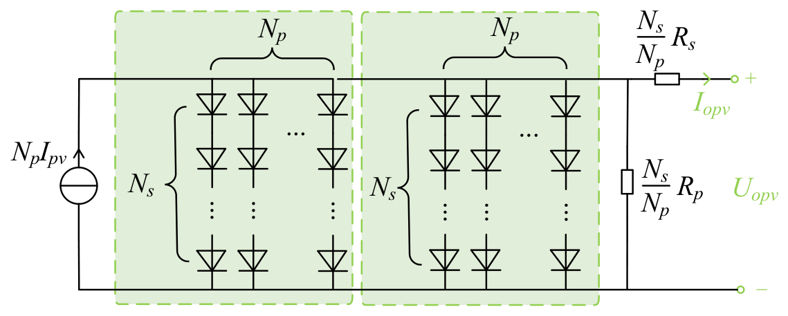
To represent the electrical behavior of a PV generator, we employ the widely used two-diode equivalent circuit, which incorporates a series resistance Rs and a shunt resistance Rp to account for internal ohmic and leakage losses [25]. The PV array consists of Ns series-connected and Np parallel-connected identical submodules, yielding the equivalent circuit depicted in Figure 5.
For the two-diode model, the current–voltage (IU) relationship is inherently nonlinear and cannot be expressed in explicit form. Instead, it is governed by the following implicit equation:
I o p v = N p I p v F p v l F p v r 1 R h U o p v N s + I o p v R s N p ,
where
F p v l = I s 1 e q k T d ( U o p v N s + I o p v R s N p ) 1 ,
F p v r = I s 2 e q A k T d ( U o p v N s + I o p v R s N p ) 1 .
where Is1 and Is2 represent the left and right diode array branch currents in Figure 5, respectively, and Fpvl and Fpvr represent the series diode volt-ampere characteristic equations. Ref. [26] proposes a correction method based on temperature and irradiance, so that the photogenerated current source Ipv of the PV is determined by the irradiance SOL and the temperature Td, which are related to each other as:
I p v = S O L S O L r e f I p v r e f + C T T d T r e f .
Finally, the actual output of the PVs goes through first-order filtering into the DC-DC converter into the DC bus.

4. LSTM Method Design with Joint SC-GFC Control

4.1. The Working Principle of LSTM

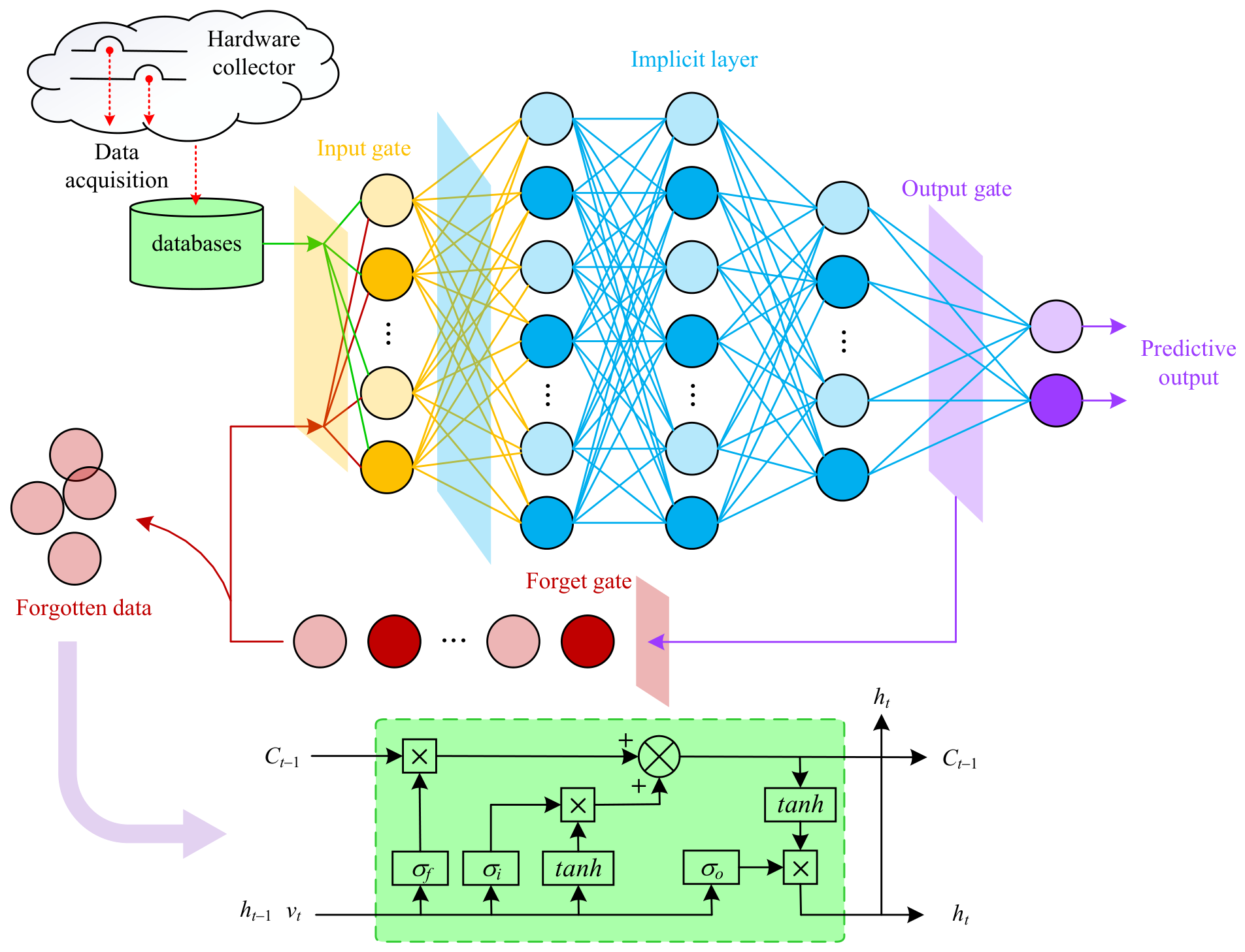
In this work, an LSTM network is employed to predict the DC bus voltage (Udc), which is critically linked to the power balance and the state of the energy storage device [27]. It is worth noting that in this paper, the input to the LSTM is the historical time series of the DC bus voltage Udc, and the output is the predicted value of Udc for one or more future time steps. LSTM, as a recurrent neural network variant specialized in processing time series data, has good long-term memory and has potential applications in time series prediction. The structure of an LSTM network consists of multiple storage cells, each containing three main gating mechanisms: an input gate, a forgetting gate, and an output gate. Within each memory cell, three gating units regulate the information flow: the input gate decides which new information should be stored; the forget gate selectively discards outdated information from the previous state; and the output gate determines which portion of the current cell state is passed to the subsequent layer. The state update of the LSTM network is shown in Figure 6.
In this paper, the input to the LSTM is the historical time series of the DC bus voltage, and the output is a representation of short-term future trends (which, after weighting, serves as a feedforward compensation signal). This design philosophy differs fundamentally from traditional voltage prediction:
The goal of traditional prediction is to replace measured values with predicted values in the control loop, which carries a high risk in practical engineering applications.
The objective of trend-aware control in this paper is to retain the feedback control based on measured values while adding an additional feedforward channel. This allows the SC to anticipate impending disturbance trends in advance, thereby enabling proactive intervention before the voltage deviates significantly from the reference value.
Therefore, the LSTM output is not used directly as a control command but is instead weighted and fused with the measured voltage value (see Section 4.3 for details), achieving coordinated control through the integration of feedback and feedforward mechanisms.
  • Oblivion gate
The forgetting gate determines whether the state information of the previous moment has been forgotten or not:
f t = S σ f h t 1 v t T + b f
where ft is the output of the forgetting gate; σf and bf are the weight and bias of the forgetting gate, respectively; ht−1 and vt are the memorized information of the previous moment and the input data of the current moment, respectively; S is the Sigmoid activation function. It is worth noting that in this paper, the input to the LSTM is the historical time series of the DC bus voltage Udc, and the output is the predicted value of Udc at one or more future time steps.
2.
Input Gate
Determines how the relevant information of the current input updates the memory cell:
i t = S σ i h t 1 v t T + b i
C ˜ t = tan h σ C h t 1 v t T + b C
where it is the output of the input gate; is the candidate memory state; σi, σC, bi and bC are the corresponding weights and biases.
3.
Memory Unit Update
Update the current memory state:
C t = f t C t 1 + i t C ˜ t
4.
Output Gate
Determines the output of the memory cell:
o t = S σ o h t 1 v t T + b o
h t = o t tan h C t
where ot is the output of the output gate; σo and bo are the weight and bias of the oblivion gate, respectively; and ht is the memory information of the current moment.
For the DC bus voltage prediction task, the input to the LSTM is a historical time series of the DC bus voltage Udc. The input vector V = [v1, v2, …, vn]T is defined as n consecutive sampling points of Udc. The target output vector Y = [y1, y2, …, yn]T represents the predicted future values of Udc for the corresponding n time steps.
The LSTM network is trained to minimize the prediction error, with the Root Mean Square Error (RMSE) serving as the loss function:
RMSE = 1 T t = 1 n v t y t 2
The optimization method used for LSTM networks is usually the Adam optimization algorithm with an update rule:
ξ t + 1 = ξ t η m t d t + ε
where ξt is the parameter at the current moment; η is the learning rate; mt and dt are the gradient mean and variance; and ε is a very small constant that prevents the denominator from being zero.

4.2. LSTM Based DC Bus Voltage Prediction

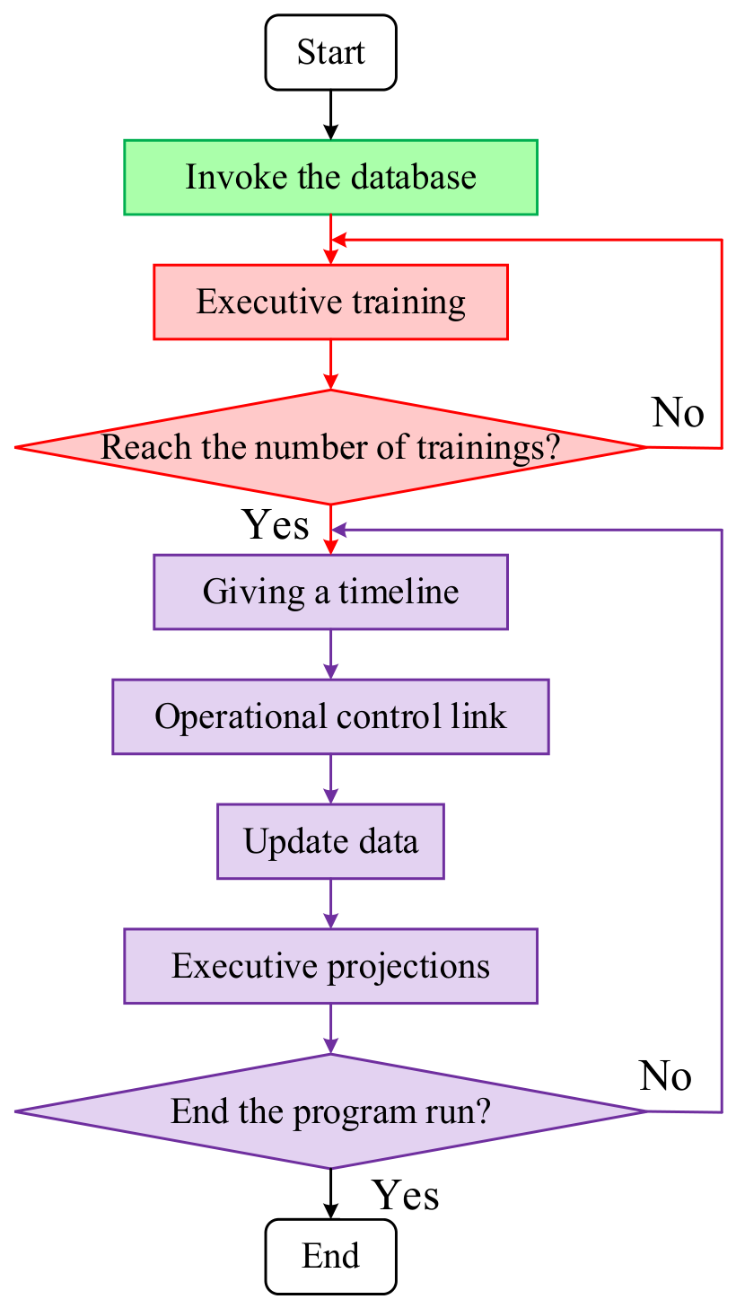
The flowchart for realizing LSTM-based DC bus voltage prediction is shown in Figure 7. First, the original database needs to be established, which is constructed in this paper using the data obtained from laboratory measurements. Subsequently, the LSTM model is trained based on the DC bus voltage data in the original database. The model training process will be described in detail in Section 5.1. After completing the model training, we will redefine the inputs of the system as follows:
Step 1: Continuous Sampling. Whether in an offline simulation, real-time simulation, or physical experimental environment, continuous sampling collects Udc data at a preset time step. Each time a new data point is collected, the historical data window is updated to form the input sequence for the current time step.
Step 2: Trend Calculation. The input sequence is fed into the trained LSTM model, and the output values are obtained through forward propagation. This output value reflects the model’s prediction of the Udc trend over the next 5–20 sampling points.
Step 3: Weighted fusion. The trend value output by the LSTM is weighted with the current measured Udc value according to preset weights w1 (measured weight) and w2 (trend weight), yielding a fused voltage signal that serves as the input reference for the SC voltage inner loop. The basis for weight selection will be discussed in Section 4.4.
Step 4: Assign a time series. In this step, the data obtained from the prediction is re-entered into the control link. In order to ensure the synchronization of system operation, it is necessary to assign the corresponding time axis or time stamp to the output data according to the time step of continuous sampling, so as to maintain the time consistency between the data and system operation.

4.3. Joint Control Strategy of SC-GFC

The joint SC-GFC control strategy enhances the conventional SC control by incorporating two additional signals derived from the GFC’s inertial response. In addition, the result of LSTM is weighted with the collected value of energy storage output voltage and incorporated into the voltage input of SC control. The structure of the control strategy is shown in Figure 8.
Notice in Figure 8 that the number of power inputs for the SC-GFC has increased from two to four, meaning that both the theoretical and measured values of inertial power are now included. We include the inertial power in the category of small signals, so the active power small signal of (1) is:
Δ P v = Im Y l E v E p Y l 2 Δ δ = M Δ δ
So, considering the action of the first order filter, the transfer function of the inertial power is:
Ψ s = M ω r e f s J v s + D v s + ω f + M ω f
Define the excitation function:
α t = P r e f + t = t 0 P r e f t = t 0 , t t 0 ε , t 0 + ε 0 , others
where t0 represents the moment of GFC response scheduling; the superscript “+” represents the right limit and “−” represents the left limit. The theoretical value of inertial power ψ t | P r e f can be obtained by converting Ψ(s) to the time-domain form ψ(t) and bringing in α(t) as the excitation. Here, α(t) is defined as a unit step function representing the step change in the active power reference Pref at the scheduling instant t0, i.e., α(t) = 0 for t < t0 and α(t) = 1 for tt0. The theoretical inertial power ψ t | P r e f is then obtained by transforming the transfer function Ψ(s) in (24) to its time-domain impulse response ψ(t), and subsequently convolving it with the excitation. This convolution yields the time-domain inertial power waveform under a step change in Pref, which is used as the theoretical reference in the joint control scheme.

4.4. Parameter Design Principles and Stability Considerations

The SC-GFC joint control strategy includes two key adjustable parameters: weights w1 and w2 (where w1 + w2 = 1), which represent the respective contribution ratios of measured voltage feedback and LSTM trend feedforward to voltage control.
Parameter selection criteria: The values of w1 and w2 must strike a balance between response speed and system stability.
Increasing w2 (i.e., increasing the feedforward weight) allows the SC to respond more sensitively to voltage trend changes, enabling rapid intervention at the onset of disturbances, which helps reduce voltage overshoot. However, an excessively large w2 will amplify noise or prediction errors in the LSTM output, introducing unnecessary control fluctuations and potentially leading to high-frequency oscillations.
Conversely, increasing w1 (i.e., increasing the feedback weight) makes the system more reliant on measured values, resulting in a smoother control process, but with a relatively slower response to disturbances.
From a control theory perspective, the proposed strategy can be viewed as adding a feedforward compensation channel to the traditional dual-loop feedback control. The trend signal from the LSTM output is essentially an advance estimate of disturbances. Introducing it as a reference value into the voltage inner loop is equivalent to pre-adjusting the duty cycle before the disturbance arrives, thereby enhancing the system’s disturbance suppression capability. The introduction of the feedforward channel does not alter the pole distribution of the closed-loop system, as the feedforward is not within the feedback loop and thus does not reduce the system’s phase margin; however, it can effectively improve the system’s response speed to specific disturbance patterns.
It should be noted that the optimal weighting coefficients may vary with operating conditions, as the LSTM’s prediction accuracy and the required inertial power support depend on the actual system state. Although this paper uses fixed weights to validate the feasibility of the hybrid framework, a simple adaptive rule can be easily implemented in actual deployment. For example, when the real-time LSTM prediction error within a sliding window exceeds a preset threshold, the feedforward weight w2 can be reduced to prevent unreliable trend information from being fed into the control loop; conversely, when the measured DC bus voltage deviation increases rapidly, w2 can be increased to enhance feedforward compensation and suppress overshoot. Systematic weight tuning strategies based on Bayesian optimization or reinforcement learning represent promising future research directions.

5. Experimental Validation

5.1. Training Process

We collected Udc data from a DC bus during steady state operation of battery charging and discharging at the DC microgrid laboratory at Hebei University of Science and Technology. The lab is equipped with a large Li-ion battery bank experimental equipment and connected to a photovoltaic array located on the roof. Based on the collected data, we built an LSTM network for predicting the future trend of Udc. The entire model training and prediction process was conducted on a personal computer using MATLAB 2023b. The first 40% of the collected data samples corresponded to the discharged state of the battery, and the second 60% of the data corresponded to the charged state of the battery. The model validation uses the latter 20% of the data samples, which mainly cover the operating state of the battery charging phase.
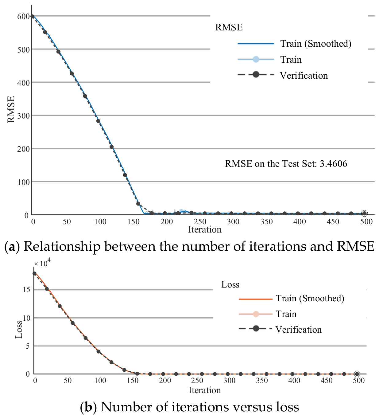
The LSTM training parameters are shown in Table 2. Based on the data of SC running in charging mode, the RMSE and loss are shown in Figure 9.
As shown in Figure 9, both the RMSE and the loss function converge and approach zero, indicating a stable and effective model training process. There is no obvious difference between the training results and the validation results, which fully verifies the high accuracy and good generalization ability of the established LSTM model in the voltage prediction task. In addition, the training results of the LSTM model also show consistent performance with the above conclusions for both the data collected from the SC running in charging and discharging modes, which further proves the robustness and reliability of the model under different operating conditions. Therefore, the trained LSTM model is able to predict the future voltage data of Udc more accurately.
To provide a quantitative benchmark, the LSTM predictor was compared with two simpler baseline methods: the second-order autoregressive (AR(2)) model and the Kalman filter. The AR(2) model was fitted using the Yule-Walker method on the same training set, while the Kalman filter was implemented using a random walk state-space model, with the noise statistics estimated from the training data. As shown in Table 3, the LSTM achieved the lowest RMSE and MAPE on the test set, with reductions of approximately 1.24% compared to the AR(2) baseline and approximately 28% compared to the Kalman filter. These results confirm that the LSTM’s ability to model nonlinear time series leads to a significant improvement in accuracy compared to linear baselines, validating its suitability as a feedforward predictor within the proposed hybrid control framework.
According to Table 3, under near-steady-state conditions, the improvement in RMSE achieved by LSTM compared to the AR(2) baseline is relatively modest, which is in line with expectations. This is expected, as the AR(2) model is inherently a linear predictor that captures only the second-order temporal correlation, making it adequate for slowly varying signals. In contrast, the LSTM is a nonlinear recurrent architecture with internal memory states that can capture long-term dependencies and abrupt pattern changes. The advantage of LSTM becomes particularly evident when the system experiences rapid transients, strong disturbances, or non-stationary behavior—conditions under which linear predictors inherently lag behind due to their limited structural flexibility.

5.2. Experimental Design

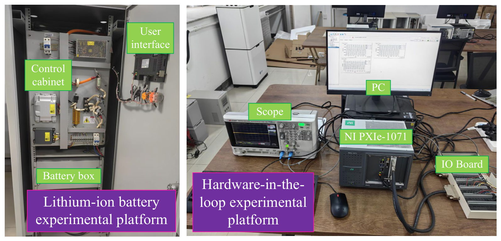
The hardware-in-the-loop (HIL) model we use is the NI PXIe-1071, a device manufactured by National Instruments (China) and distributed by Modeling Tech (Shanghai, China). This device can simulate the main circuit topology required for this paper. We built PVC, GFC and SC models in the main circuit of the HIL. The third-order dynamic modeling of PV devices and energy storage devices is also built in the control loop, which is realized by controlled sources. The photo of the experimental platform we used is shown in Figure 10. The main circuit parameters are shown in Table 4; the control circuit parameters are shown in Table 5, where Udc,ref is the DC bus reference voltage.
The main circuit simulation step of HIL is fixed to be 2 μs, and the sampling frequency and control frequency are 10 kHz. In order to validate the method described in this paper, we designed the following experiments:
  • Validation of SC-GFC joint control: The SC is operated in both charging and discharging modes, and the system’s power and frequency response are observed by adjusting Pref and Qref.
  • Verify the hybrid driving effect of LSTM with the control system: we adjust the weights w1 and w2, and observe the variation in the DC bus voltage at steady state.
During the experiment, the current limit of PVC follows the variation in Pref, while the GFC is able to absorb reactive power from the grid side. During steady-state operation, the GFC will always maintain network-forming control, and there will be no switching between control modes during this period. The SC and PVC will always maintain constant-power control, and the control structure will remain unchanged.
To verify the real-time feasibility of LSTM-enhanced control, the LSTM forward inference time was measured on an NI PXIe-1071 platform. The average inference time per prediction step was approximately 0.021 s, with the weight optimization and weighted fusion update periods both maintained at a constant 1.0 s. Considering the pulse-width modulation frequency and the typical control cycle tolerance for DC bus regulation, the LSTM inference delay was well within an acceptable range. This confirms that the proposed hybrid control can be executed in real time without compromising the system’s dynamic response.

5.3. Joint Control Verification of SC-GFC

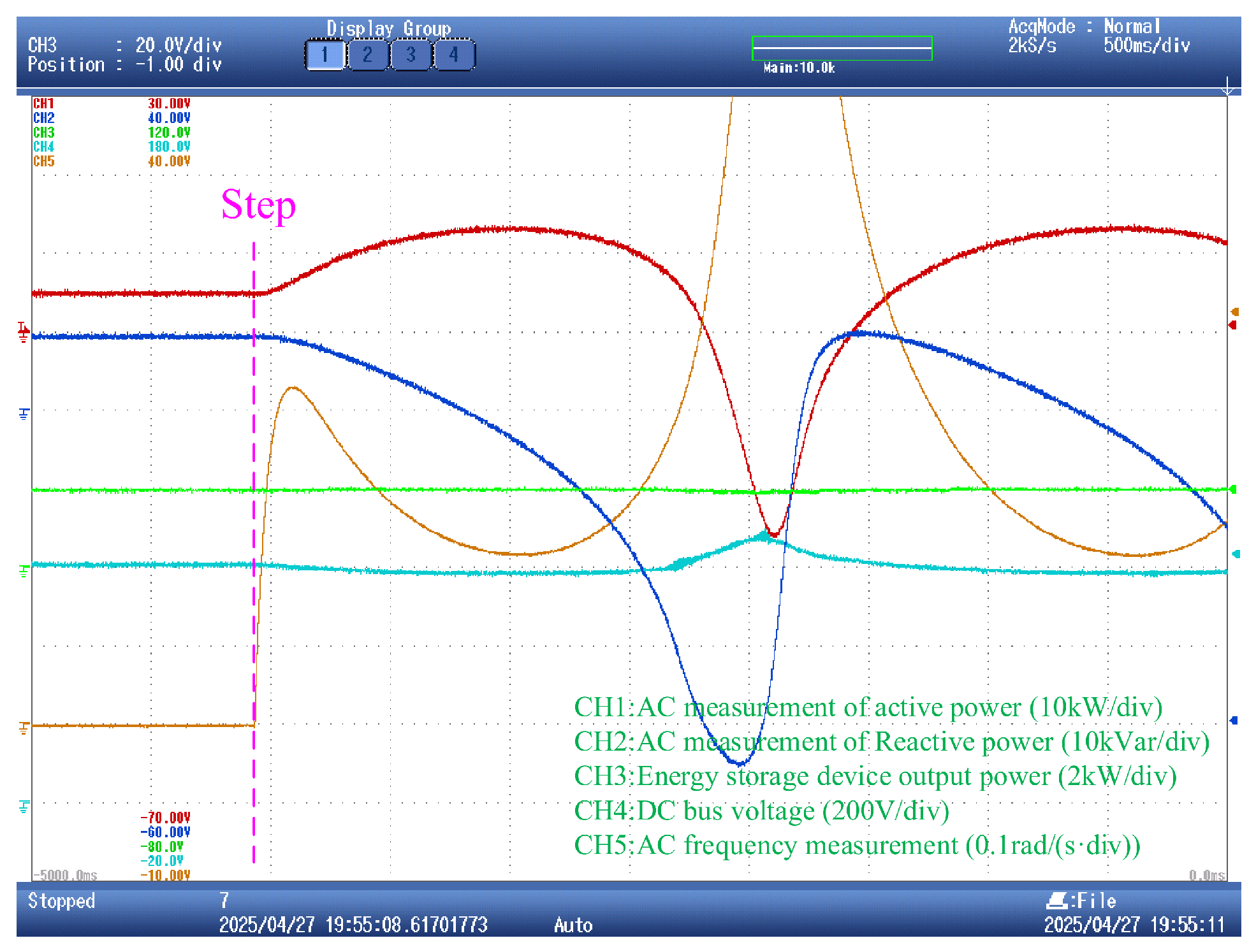
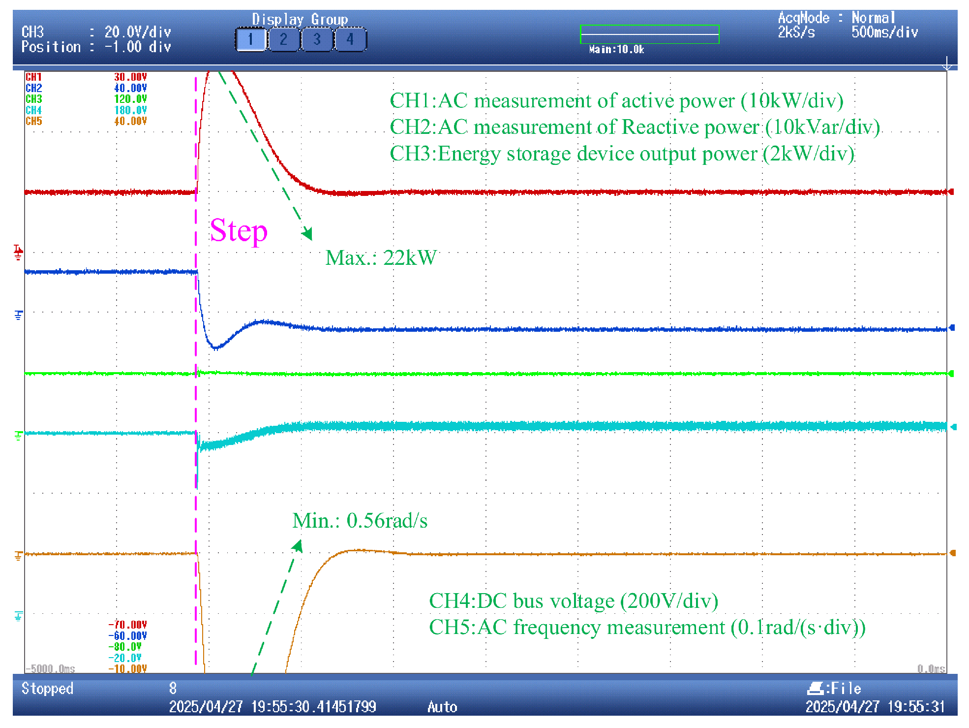
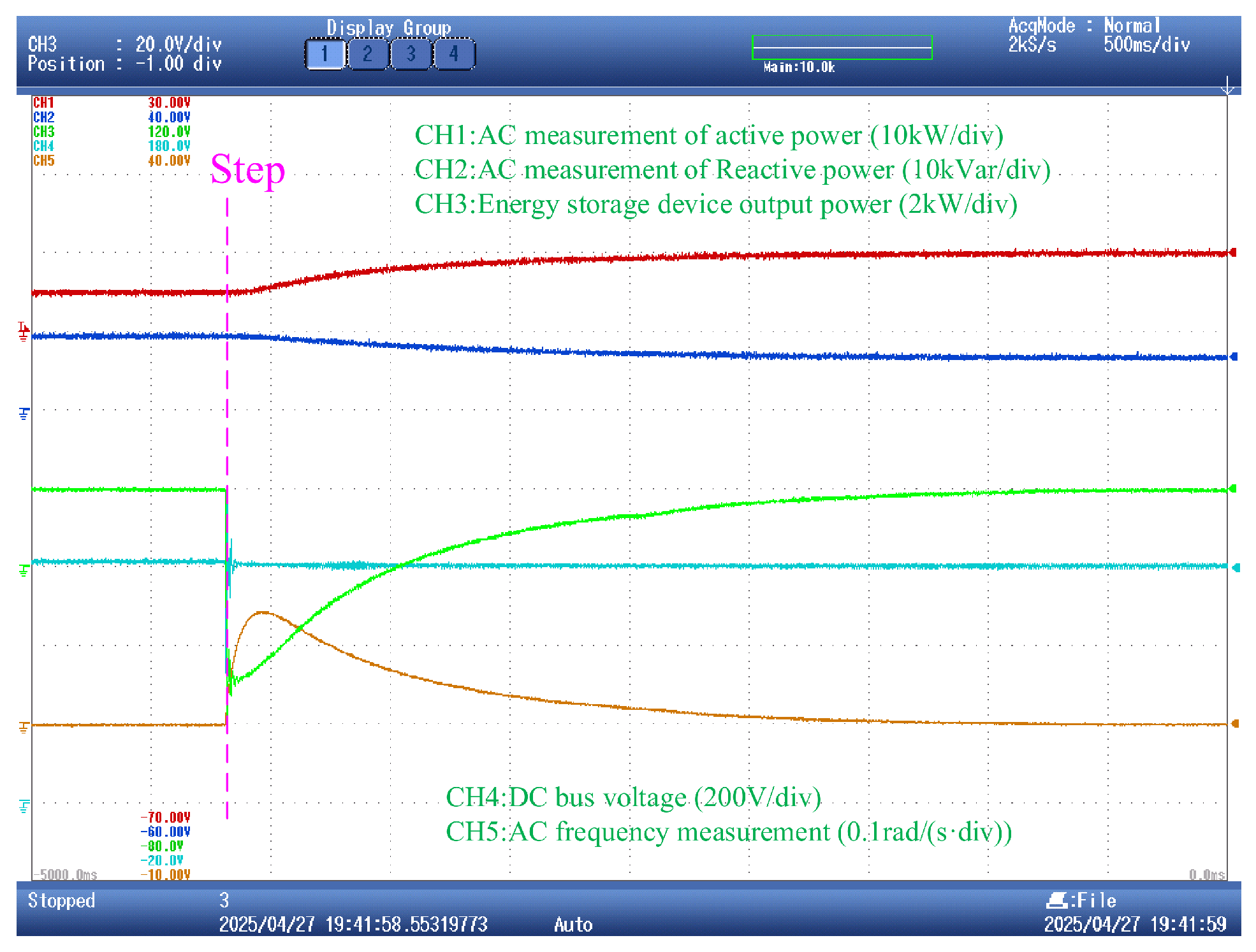
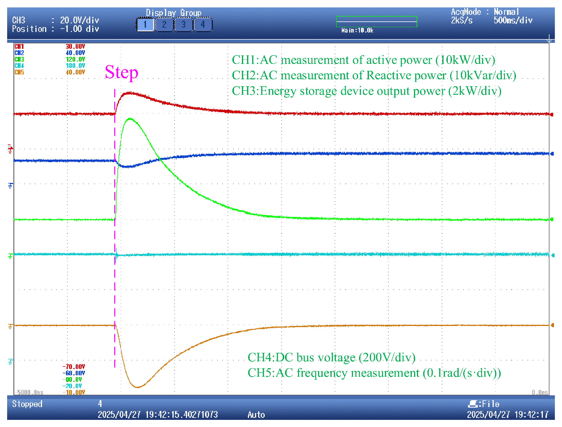
When the SC works in charging mode, Pce,ref is fixed at −2000 W; when the SC works in discharging mode, Pce,ref is fixed at +2000 W. A step change in Pref from 5 kW to 10 kW is applied, and the waveforms of Pv, Qv, Pce, Udc, ωv are observed. The control parameters including LSTM weights are consistent with Table 3. For comparison, a benchmark case with independently controlled converters (without the LSTM enhancement) is implemented, which is switched to independent control by the joint control to make it run to stability. First in the discharge mode, we observe the operating effects of the SC-GFC joint control and independent control, as shown in Figure 11 and Figure 12.
An examination of the results in Figure 11 and Figure 12 reveals that, when using SC-GFC combined control, the active power and frequency of the GFC converge, and the SC responds perfectly to the GFC’s inertial power. However, under independent control, adjustments to the active power reference not only fail to converge but also generate significant low-frequency oscillations. In these figures, the operating modes are clearly labeled: the GFC is in grid-forming mode, while the SC is in constant-power charge–discharge mode. To facilitate quantitative comparison on a compressed scale, key transient peaks are directly labeled on the waveforms. The low-frequency oscillations observed under independent control are consistent with the instability mechanism reported in the literature [6,7,8], namely, a lack of dynamic power coordination between the DC power source and the GFC, leading to persistent oscillations in the power-phase angle. This confirms that a fixed-power SC inherently lacks the ability to meet the GFC’s inertial power demand.
To verify the inertial power transfer function Ψ(s) derived in Equation (24), we compared the theoretical step response of this function with the inertial power measured from the SC during the Pref step transient (5 kW → 10 kW). The theoretical response was obtained by applying the inverse Laplace transform to Ψ(s) under the same step excitation. As shown in Table 6, the steady-state error between the theoretical value and the measured inertial power is within 5%, and the settling time deviation is less than 0.5 s. This high degree of agreement confirms that the derived transfer function accurately captures the dynamic characteristics of the GFC system’s inertial power.
The slight deviation between the theoretical value and the measured steady-state value stems from differences in the types and precision of the solvers used in the transfer function simulation and the HIL platform. The transfer function simulation employed a continuous-domain solver, while the HIL platform used a discrete fixed-step solver, which introduced minor quantization and discretization errors. However, the overall error was within 5%, confirming the validity of the derived transfer function.
Again in SC discharge mode, we adjust Qref from 0 kVar to 5 kVar and observe the system changes as shown in Figure 13 and Figure 14.
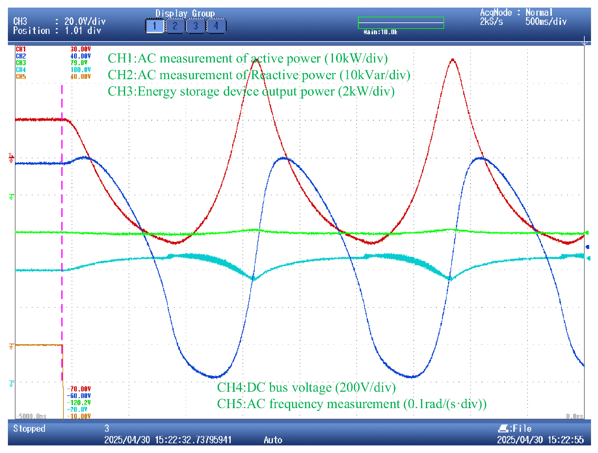
We can observe that when adjusting the reactive power reference value, the transient fluctuations under independent control are significantly higher than those under SC-GFC joint control. In Figure 14, CH1 exceeds the original evaluation range due to severe fluctuations. To clearly illustrate the actual transient behavior, the true peak values reached during the instability period are directly labeled in the figure. This saturation/out-of-range phenomenon intuitively demonstrates that independent control enters a deep instability region under a reactive power step. In contrast, the proposed SC-GFC joint control remains within the stable operating range at all times. In the control group, it can be observed that when the reactive power is altered, the GFC operating mode shifts from the first quadrant to the fourth quadrant, indicating that the GFC begins to draw reactive power from the grid to maintain the stability of the DC bus voltage. The SC-GFC joint control, however, does not face this issue; the DC bus voltage remains stable even during the inertial active power response.
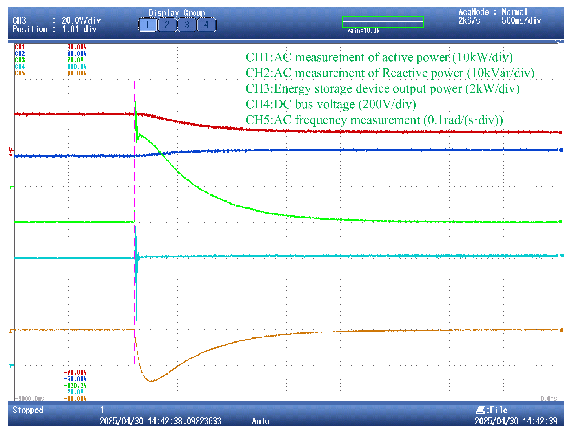
If the SC is in charging condition, we make Pref step from the steady state of 10 kW to 5 kW, and observe the waveforms of Pv, Qv, Pce, Udc and ωv as Figure 15 and Figure 16. We are also able to get the same conclusion in the discharge mode.
Similarly, in charging mode, we arrive at the same conclusions as in discharging mode. The independent control once again exhibits severe transient fluctuations, while the proposed joint control is able to maintain stable operation. The transient peaks of some of the curves are labeled in the figure to facilitate quantitative comparison.
Therefore, the proposed joint SC-GFC control is essential for achieving stable grid-forming operation in hybrid PV-energy storage systems.

5.4. Verification of Hybrid Driving of LSTM with Control Link

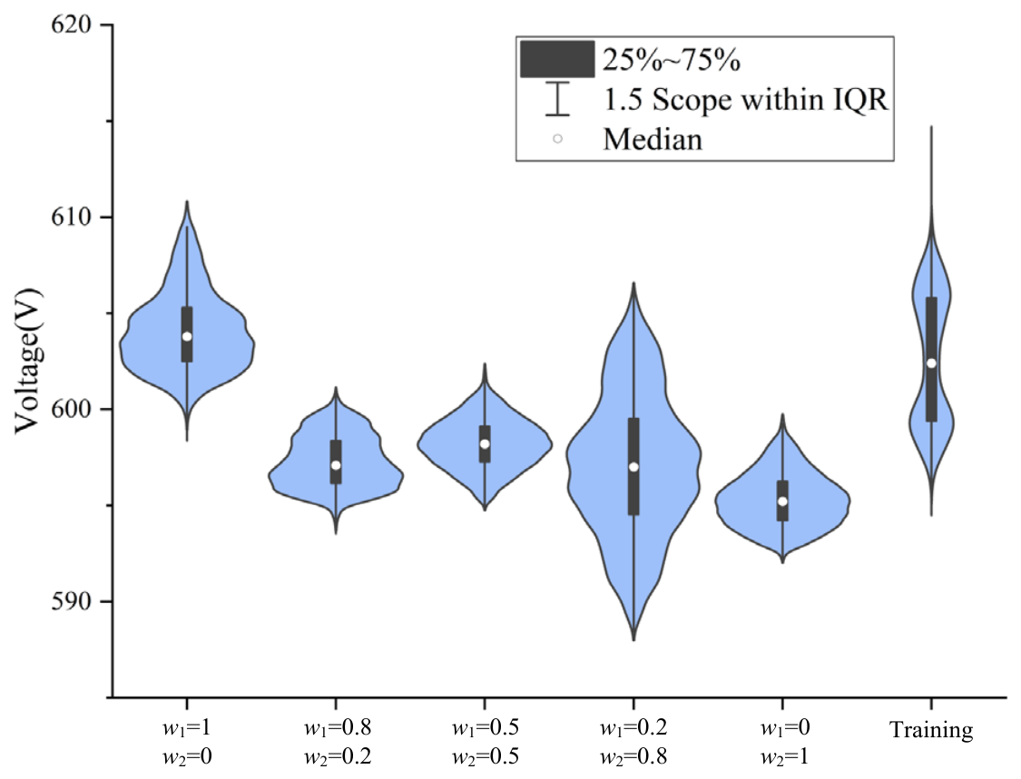
To verify the hybrid driving effect of the LSTM integrated with the control system, the weights w1 and w2 are adjusted, and the resulting changes in the DC bus voltage are observed. the SC maintains the charging mode of −2000 W, and both Pref and Qref are fixed at 10 kW and 5 kVar. We intercept the DC bus voltage waveforms for 3 s at a sampling frequency of 0.1 kHz, and include the training dataset into it as well. The distribution of the collected values of the DC bus voltage is shown in Figure 17.
To isolate the contribution of the LSTM feedforward path, the baseline case—which does not include the LSTM—is represented by the weight settings (w1 = 1, w2 = 0). This simplifies the proposed hybrid control to pure feedback control (i.e., using only the measured Udc in the SC voltage loop). This baseline case employs the same experimental conditions, SC-GFC joint control architecture, and PI parameters as the proposed method, thereby ensuring a fair comparison. As shown in Figure 17, the center of the Udc distribution under the baseline case (w1 = 1) lies above 600 V and exhibits greater dispersion, indicating a larger steady-state deviation. In contrast, when LSTM feedforward with appropriate weights is enabled (e.g., w1 = w2 = 0.5), the voltage distribution shifts below 600 V and becomes more concentrated. This direct comparison confirms that the LSTM feedforward path—rather than the joint control architecture alone—is the key factor in improving steady-state performance.
In summary, the proposed physics-data fusion framework, combining the LSTM-based feedforward with the physical joint-control law, has been validated through the above experimental results, demonstrating its effectiveness in improving steady-state performance.

5.5. Explanation of Operating Power and Robustness Against Real-World Disturbances

(1)
Remark on operating power levels
The experiments in this section are conducted at representative power levels (5 kW → 10 kW and 10 kW → 5 kW), which cover both upward and downward step changes around the typical operating point. The proposed joint control strategy is structurally independent of the absolute power level: the GFC inertial power demand is linearly proportional to the frequency deviation and is fed back to the SC power reference regardless of the steady-state power level. Therefore, the dynamic coordination mechanism remains effective across a wide range of operating conditions. While additional tests at 25% and 75% rated power would provide further quantitative evidence, the current results at two distinct power levels (covering the most critical transient scenario) sufficiently demonstrate the effectiveness of the proposed scheme. A systematic sweep across multiple power levels is planned for future experimental work.
(2)
Remark on robustness to realistic disturbances
The proposed method is designed to address the fundamental issue of dynamic power mismatch between the GFC and the source-side SC, rather than to track specific external disturbances such as PV irradiance fluctuations. The LSTM feedforward path extracts voltage trends from the DC bus itself, which inherently reflects the cumulative effect of all disturbances (including PV variations and load changes). Therefore, as long as the DC bus voltage contains the dynamic signature of the disturbance, the LSTM can provide an effective feedforward compensation. Regarding SOC variations, the SC’s dynamic response capability is reflected in its voltage-current characteristics, which are captured by the measured DC bus voltage and the power loop feedback. The proposed joint control does not require explicit SOC information; it relies on the physical response of the system, making it inherently robust to SOC changes within the normal operating range. A comprehensive experimental evaluation under time-varying PV profiles and extreme SOC conditions is deferred to future work, as the present study focuses on the core validation of the joint control framework.

6. Conclusions

Through theoretical analysis and hardware-in-the-loop experiments, the following key findings are obtained:
  • Joint SC-GFC control is essential for damping power oscillations. Under the same Pref step transient, the independent fixed-power SC control exhibits sustained low-frequency oscillations, whereas the proposed joint control achieves rapid convergence and stable power tracking. This confirms that feeding the GFC’s inertial power demand back to the SC reference is a necessary condition for stable grid-forming operation in PV-storage systems.
  • The LSTM feedforward path provides measurable steady-state improvement over pure feedback. By comparing the weight settings w1 = 1, w2 = 0 (no LSTM) and w1 = w2 = 0.5 (with LSTM), the DC bus voltage distribution becomes more concentrated and shifts closer to the reference value when the LSTM feedforward is activated. This demonstrates that the trend-aware prediction effectively reduces steady-state deviations without relying on external communication.
  • The hybrid physical-data-driven framework offers a practical, communication-free solution. The integration of the physical joint-control law with the LSTM-based feedforward compensation is validated under both charging and discharging modes. The framework achieves a trade-off between dynamic response and steady-state accuracy through the adjustable weighting scheme, while avoiding the latency and reliability issues associated with communication-dependent data-driven methods.
Limitations regarding adaptive weight tuning under varying operating conditions and experimental validation under extreme SOC or irradiance fluctuations are acknowledged as future work.

Author Contributions

Conceptualization, Y.Q. and Y.G.; methodology, Y.G.; software, E.Z.; validation, Y.Q. and T.M.; formal analysis, D.M. and K.L.; investigation, E.Z.; resources, Y.G.; data curation, T.M.; writing—original draft preparation, Y.Q.; writing—review and editing, D.M. and Y.G.; visualization, Y.Q. and K.L.; supervision, D.M.; project administration, P.B.; funding acquisition, P.B. and Y.G. All authors have read and agreed to the published version of the manuscript.

Funding

This work is Supported by S&T Program of Hebei (23284502Z) and Hebei Natural Science Foundation (E2025208078).

Data Availability Statement

The original contributions presented in this study are included in the article. Further inquiries can be directed to the corresponding author.

Conflicts of Interest

Author Dabin Mi, Tao Ma, Kun Li were employed by the company Hebei Province Construction & Investment Group Co., Ltd. Author Erhui Zhang was employed by the company Hebei Suntien New Energy Technology Co., Ltd. Author Pengyu Bai was employed by the company Suntien Green Energy Co., Ltd. The remaining authors declare that the research was conducted in the absence of any commercial or financial relationships that could be construed as a potential conflict of interest.

References

  1. Chi, Y.; Jiang, B.; Hu, J.; Lin, W.; Liu, H.; Fan, Y.; Ma, S.; Yao, J. Grid-forming Converters: Physical Mechanism and Characteristics. High Volt. Eng. 2024, 50, 590–604. [Google Scholar]
  2. Karunaratne, L.; Chaudhuri, N.R.; Yogarathnam, A.; Yue, M. Nonlinear Backstepping Control of Grid-Forming Converters in Presence of Grid-Following Converters and Synchronous Generators. IEEE Trans. Power Syst. 2024, 39, 1948–1964. [Google Scholar] [CrossRef] [Scilit]
  3. Gong, X.; Wang, X.; Cao, B. On Data-Driven Modeling and Control in Modern Power Grids Stability: Survey and Perspective. Appl. Energy 2023, 350, 121740–121758. [Google Scholar]
  4. Guo, Y.; Qi, Y.; Ge, L.; Hou, L.; Li, J.; Sun, H. Transient Compensation of Asymmetrical Line Faults in Multigrid-Forming VSG Systems. IEEE Trans. Ind. Electron. 2025, 72, 10085–10096. [Google Scholar] [CrossRef] [Scilit]
  5. Cao, W.; Qin, H.; Lu, J.; He, B.; Zhuang, K.; Li, G. Orientation and Application Prospect of Virtual Synchronous Generator in New Power System. Autom. Electr. Power Syst. 2023, 47, 190–207. [Google Scholar]
  6. Lei, J.; Xiang, X.; Liu, B.; Li, W.; He, X. Quantitative and Intuitive VSG Transient Analysis with the Concept of Damping Area Approximation. IEEE Trans. Smart Grid 2023, 14, 2477–2480. [Google Scholar] [CrossRef] [Scilit]
  7. Me, S.P.; Ravanji, M.H.; Mansour, M.Z.; Zabihi, S.; Bahrani, B. Transient Stability of Paralleled Virtual Synchronous Generator and Grid-Following Inverter. IEEE Trans. Smart Grid 2023, 14, 4451–4466. [Google Scholar] [CrossRef] [Scilit]
  8. Qin, B.; Xu, Y. Modal Analysis of Multi-virtual Synchronous Machine Grid-connected Power-frequency Oscillation. Proc. CSEE 2021, 41, 6570–6581. [Google Scholar]
  9. Ge, P.; Tu, C.; Xiao, F.; Ge, P.; Tu, C.; Xiao, F.; Guo, Q. Transient Stability Enhancement of a VSG Based on Flexible Switching of Control Parameters. Proc. CSEE 2022, 42, 2109–2124. [Google Scholar]
  10. Cheng, H.; Li, C.; Ghias, A.M.Y.M.; Blaabjerg, F. Dynamic Coupling Mechanism Analysis Between Voltage and Frequency in Virtual Synchronous Generator System. IEEE Trans. Power Syst. 2024, 39, 2365–2368. [Google Scholar] [CrossRef] [Scilit]
  11. Yang, M.; Wang, Y.; Xiao, X.; Li, Y. A Robust Damping Control for Virtual Synchronous Generators Based on Energy Reshaping. IEEE Trans. Energy Convers. 2023, 38, 2146–2159. [Google Scholar] [CrossRef] [Scilit]
  12. Wang, Z.; Chen, Y.; Li, X.; Xu, Y.; Luo, C.; Li, Q.; He, Y. Active Power Oscillation Suppression Based on Decentralized Transient Damping Control for Parallel Virtual Synchronous Generators. IEEE Trans. Smart Grid 2023, 14, 2582–2592. [Google Scholar] [CrossRef] [Scilit]
  13. Wang, W.; Shi, X.; Wu, G.; Cao, Y. Interaction Between Grid-Forming Converters with AC Grids and Damping Improvement Based on Loop Shaping. IEEE Trans. Power Syst. 2024, 39, 1905–1917. [Google Scholar] [CrossRef] [Scilit]
  14. Zheng, L.; Liu, X.; Xu, Y.; Hu, W.; Liu, C. Data-driven Estimation for a Region of Attraction for Transient Stability Using the Koopman Operator. CSEE J. Power Energy Syst. 2023, 9, 1405–1413. [Google Scholar] [CrossRef] [Scilit]
  15. Wang, Z.; Li, G.; Huang, Z.; Zhang, X.; Xu, Y.; Zheng, L. Physics Informed Data-Driven Oscillation Stabilization Strategy for Renewable-Dominant Power Systems Based on Koopman Operator. IEEE Trans. Ind. Appl. 2025, 61, 2632–2645. [Google Scholar] [CrossRef] [Scilit]
  16. Shuai, H.; She, B.; Wang, J.; Li, F. Safe Reinforcement Learning for Grid-forming Inverter Based Frequency Regulation with Stability Guarantee. Mod. Power Syst. Clean Energy 2025, 13, 79–86. [Google Scholar] [CrossRef] [Scilit]
  17. Fahad, S.; She, B.; Yin, J.; Li, F.; Cui, H.; Bo, R. A Data-Driven Adaptive Control Approach for Enhancing the Dynamic Response of VSGs in Varying Grid Conditions. IEEE Trans. Power Deliv. 2025, 40, 1421–1433. [Google Scholar] [CrossRef] [Scilit]
  18. Cavus, M.; Jiang, J.; Allahham, A. Deep Multi-Task Forecasting of Net-Load and EV Charging with a Residual-Normalised GRU in IoT-Enabled Microgrids. Energies 2026, 19, 311. [Google Scholar] [CrossRef] [Scilit]
  19. Rojas, C.A.; Kouro, S.; Inzunza, R.; Mitsugi, Y.; Alcaide, A.M. Harmonic Impedance Model of Multiple Utility-Interactive Multilevel Photovoltaic Inverters. Energies 2022, 15, 9462. [Google Scholar] [CrossRef] [Scilit]
  20. Shen, X.; Liu, J.; Lin, H.; Yin, Y.; Alcaide, A.M.; Leon, J.I. Cascade Control of Grid-Connected NPC Converters via Sliding Mode Technique. IEEE Trans. Energy Convers. 2023, 38, 1491–1500. [Google Scholar] [CrossRef] [Scilit]
  21. Bevrani, H.; Ise, T.; Miura, Y. Virtual synchronous generators: A survey and new perspectives. Int. J. Electr. Power Energy Syst. 2014, 54, 244–254. [Google Scholar] [CrossRef] [Scilit]
  22. Salameh, Z.M.; Casacca, M.A.; Lynch, W.A. A mathematical model for lead-acid batteries. IEEE Trans. Energy Convers. 1992, 7, 93–98. [Google Scholar] [CrossRef] [Scilit]
  23. Oh, D.; Jeon, J.; Kim, M.; Lee, W.; Lim, J.; Hong, J. A computationally efficient physics-based equivalent circuit model for real-time simulation of electrochemical-thermal behavior in lithium-ion batteries. Appl. Energy 2026, 426, 128608. [Google Scholar] [CrossRef] [Scilit]
  24. Pan, D.; Wang, X.; Liu, F.; Shi, R. Transient Stability of Voltage-Source Converters with Grid-Forming Control: A Design-Oriented Study. IEEE J. Emerg. Sel. Top. Power Electron. 2020, 8, 1019–1033. [Google Scholar] [CrossRef] [Scilit]
  25. Cheknane, A.; Hilal, H.S.; Djeffal, F.; Benyoucef, B.; Charles, J.P. An equivalent circuit approach to organic solar cell modelling. Microelectron. J. 2008, 39, 1173–1180. [Google Scholar] [CrossRef] [Scilit]
  26. Chenni, R.; Makhlouf, M.; Kerbache, T.; Bouzid, A. A detailed modeling method for photovoltaic cells. Energy 2007, 32, 1724–1730. [Google Scholar] [CrossRef] [Scilit]
  27. Qi, Y.; Guo, Y.; Xie, P.; Sun, H. Joint Control of Storage Voltage Prediction and Grid-forming Converter using LSTM. In Proceedings of the 2025 IEEE International Conference on Power Systems and Smart Grid Technologies (PSSGT), Chongqing, China, 11–13 April 2025; pp. 280–287. [Google Scholar]
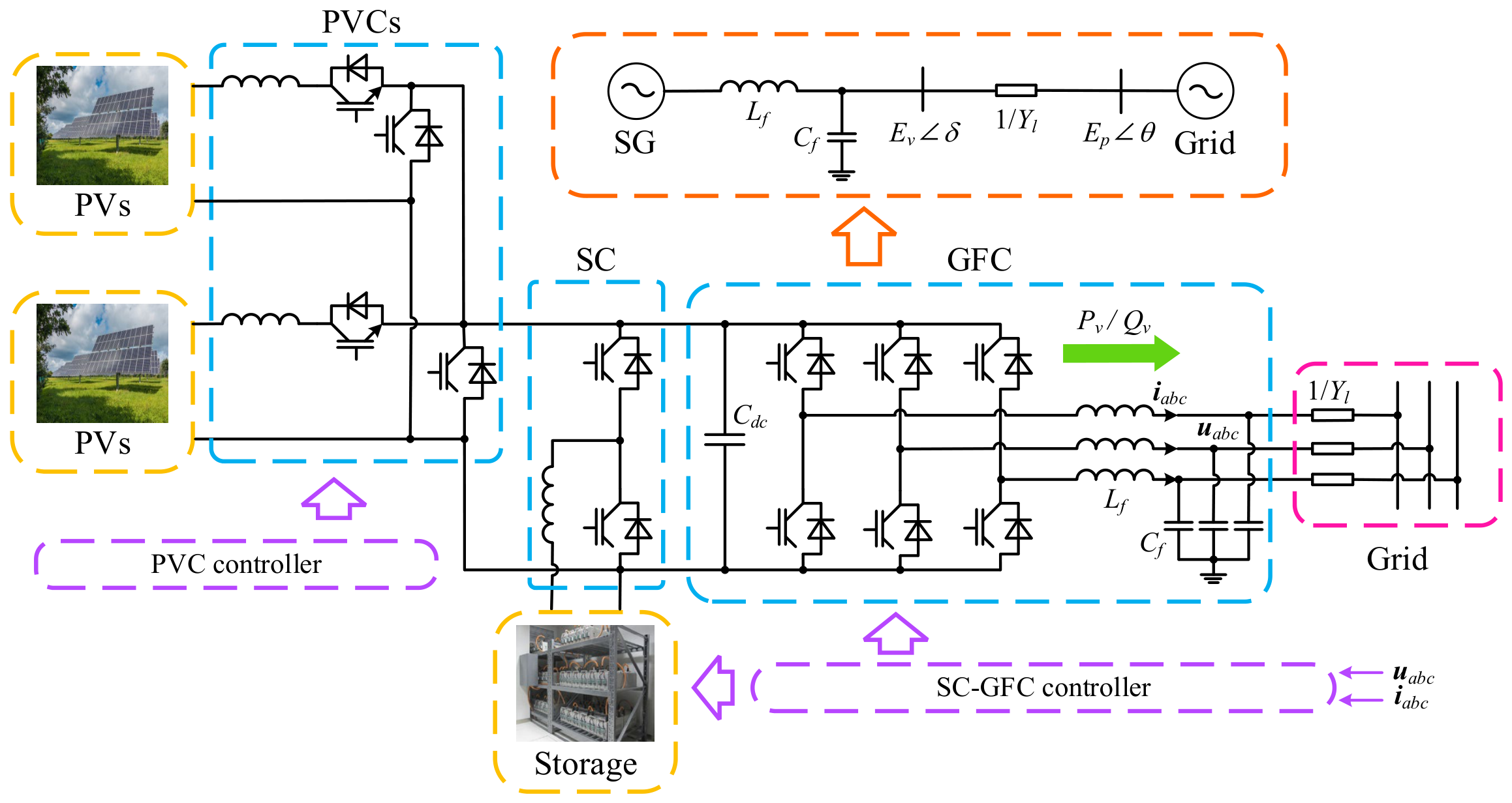
Figure 1. Topology of the system.
Electronics 15 03782 g001
Figure 2. Energy storage converter control block diagram.
Electronics 15 03782 g002
Figure 3. PV converter control block diagram.
Electronics 15 03782 g003
Figure 4. Third-order dynamic equivalent circuit for lithium-ion batteries.
Electronics 15 03782 g004
Figure 5. Two-Diode Equivalent Circuit for PV Arrays.
Electronics 15 03782 g005
Figure 6. State update method of LSTM.
Electronics 15 03782 g006
Figure 7. LSTM-based DC bus voltage prediction process.
Electronics 15 03782 g007
Figure 8. Joint SC-GFC control strategy.
Electronics 15 03782 g008
Figure 9. Training process of LSTM.
Electronics 15 03782 g009
Figure 10. Photo of experimental platform.
Electronics 15 03782 g010
Figure 11. Operational effects of SC-GFC joint control in discharge mode (Qref = 0 kVar).
Electronics 15 03782 g011
Figure 12. Operation effect of independent control in discharge mode (Qref = 0 kVar).
Electronics 15 03782 g012
Figure 13. Operational effects of SC-GFC joint control in discharge mode (Qref = 5 kVar).
Electronics 15 03782 g013
Figure 14. Operation effect of independent control in discharge mode (Qref = 5 kVar).
Electronics 15 03782 g014
Figure 15. Operation effect of SC-GFC joint control in charging mode.
Electronics 15 03782 g015
Figure 16. Operation effect of independent control in charging mode.
Electronics 15 03782 g016
Figure 17. DC bus voltage of the SC under different weights.
Electronics 15 03782 g017
Table 1. Comparison of Relevant Studies.
ReferenceControl ArchitectureData-DrivenCommunication RequiredKey Limitation
[6,7,8,9,10]GFC onlyNoNoIgnored source-side dynamic
[11,12,13]GFC with enhanced algorithmsNoNoAssumed ideal DC source
[14,15,16,17]GFC + data-driven optimizationYesYesCommunication latency risks
This workJoint SC-GFCYes
(LSTM feedforward)
NoLimited validation under extreme SOC (future work)
Table 4. Circuit Parameters.
ParametersValueParametersValue
Lf2 mHCf20 μF
Rf0.5 ΩUdc,ref750 V
Uref380 VCdc4700 μF
1/Yl0.82 + j0.454 ΩRd0.07 Ω
Rp0.11 ΩRgas18.4 Ω
Rw0.3 ΩCw22 nF
wref100π rad/s
Table 5. Controller Parameters.
ParametersValueParametersValue
Jv1 kg·m2Dv100 W·rad/s
Kqu0.1 V/Varwf10π rad/s
kpp0.5kip0.25
kpu0.6kiu0.3
kpd1kid20
kpi0.6kii0.3
w10.8w20.2
Table 6. Comparison of Inertial Power.
MetricTheoretical
(Ψ(s))
Measured
(HIL)
Steady-state inertial power0.9703 W0.9658 W
Settling time (to 5% band)3.344 s3.6 s
Peak overshoot562 W574 W
Table 2. Training Parameters of LSTM.
ParametersValue
σi = σC = σf = σo0.95
bi = bC = bf = bo0
T0.2 s
mt1
dt0
h2
Table 3. Comparison of Baseline Methods on the Test Set.
ModelRMSE (V)MAPE (%)
AR(2) baseline3.44950.51%
Kalman filter4.77370.65%
LSTM (proposed)3.40660.35%
Disclaimer/Publisher’s Note: The statements, opinions and data contained in all publications are solely those of the individual author(s) and contributor(s) and not of MDPI and/or the editor(s). MDPI and/or the editor(s) disclaim responsibility for any injury to people or property resulting from any ideas, methods, instructions or products referred to in the content.