Adaptive Hyperparameter Adjustment and Resource Allocation for Federated Learning in the Industrial Internet of Things

Abstract

Timely and accurate defect classification is critical for ensuring product quality and safety in industrial inspection scenarios. The widespread deployment of Internet of Things (IoT) devices equipped with sensing, computing, and communication capabilities has promoted the development of AI-enabled industrial applications. However, conventional AI approaches typically rely on centralized data collection and processing, which become impractical in real-world IoT environments due to growing privacy concerns and constrained device resources. To address these challenges, this paper proposes a communication-efficient adaptive federated learning algorithm for heterogeneous defect classification tasks. The proposed approach jointly accelerates the training process through three mechanisms: (i) adaptive local updates that balance communication and computation overheads; (ii) parameter compression that trades off communication cost against model accuracy; (iii) joint bandwidth and computation-power allocation that optimizes per-round communication and computation time across participating devices. We further analyze the joint effects of these three mechanisms and provide a convergence analysis. Extensive simulations show that the proposed method achieves competitive classification accuracy while reducing single-round training time by up to 70%.

1. Introduction

As a foundational element within the framework of Industry 4.0, the Industrial Internet of Things (IIoT) demonstrates remarkable promise in facilitating data-centric automation and operational control within manufacturing and industrial contexts [1]. The pervasive integration of the IIoT alongside the swift advancement of edge artificial intelligence (AI) has facilitated the connection of a large number of IIoT devices to the periphery of the Internet. Each of these devices consistently generates a large amount of data, which requires the use of deep learning (DL) methodologies for data processing to perform various tasks [2].

The conventional approach to centralized training of DL models necessitates a central server to aggregate the raw data produced by devices via wireless transmission, facilitating subsequent processing and analysis. However, in light of communication resource constraints and apprehensions regarding data privacy, it is impractical for all IIoT devices to transmit their data to a central server for the purpose of training DL models [3]. Therefore, the development of an effective and privacy-preserving distributed DL method is of great significance.

Federated learning (FL) is a promising distributed, privacy-preserving learning framework with extensive utility in IIoT domains. FL allows IIoT devices to share local model parameters instead of raw data for the collaborative training of global models, thereby addressing privacy concerns related to data sharing and reducing the communication overhead of DL model training in the IIoT [4,5]. It is important to note, however, that FL alone does not provide a complete privacy guarantee; recent studies have shown that adversaries may reconstruct training samples from shared gradients through gradient leakage attacks. To further strengthen privacy protection, complementary techniques such as secure aggregation and differential privacy can be integrated into the FL pipeline, though each introduces its own trade-offs in terms of communication overhead or model utility. In a typical industrial quality inspection scenario, multiple production lines or workshops are equipped with various inspection devices (e.g., high-resolution cameras, laser scanners, and ultrasonic sensors). These devices have different sensing, computing, and communication capabilities. These devices are often deployed in harsh environments with unstable network conditions, leading to significant heterogeneity in both hardware and communication. Moreover, data heterogeneity naturally arises because different production lines may manufacture different product types or operate under varying lighting and surface conditions, resulting in distinct defect patterns and label distributions across devices. For instance, one line may predominantly produce metal components with scratch defects, while another focuses on plastic parts with bubble or discoloration defects. This data and system heterogeneity poses substantial challenges for conventional federated learning algorithms. Additionally, applying FL to IIoT networks still faces other challenges. The number of parameters in DL models typically ranges from tens of thousands to hundreds of millions, requiring substantial communication resources for IIoT devices to update their local models. However, the operating environments of IIoT devices often constrain their communication bandwidth, posing challenges in meeting the communication demands of DL training. The disparity between the computing and storage requirements of DL models and the limited resources of IIoT devices is exacerbated by the growing complexity of DL models.

To address the above issue, many solutions have been proposed, including training local models for multiple rounds before updating their parameters, compressing local model parameters, and improving resource-allocation efficiency. Performing multiple rounds of local training improves the use of device computing power by reducing frequent model-parameter transmissions. This approach can balance computation and communication by introducing a local model update coefficient [6]. Parameter compression reduces the amount of transmitted data through compression techniques such as quantization and sparsity. A parameter-compression algorithm balances communication and model accuracy by determining the compression coefficient (quantization level), which represents the trade-off between bandwidth and accuracy [7]. Resource allocation aims to alleviate the communication bottleneck [8] and prevent devices from falling behind. Proper allocation of computing and bandwidth resources can determine the duration of a single communication round, balance communication and computation, and optimize device-side communication and computation. To improve the efficiency of federated learning, we study these methods in this paper.

The above three methods have been proven to significantly reduce communication overhead and the duration of individual federated learning rounds. However, the total time consumed by federated learning depends on two factors: (1) the number of communication rounds required to achieve the target model-convergence accuracy; (2) the duration of each communication round. These factors are interdependent and therefore require joint rather than isolated optimization. An effective solution should dynamically adjust the parameters based on historical training information to select the optimal quantization level, local update frequency, computation frequency, and bandwidth allocation, while automatically balancing communication time and model-convergence loss in each training round, thereby accelerating large-scale federated learning.

Our main contributions are summarized as follows:

• We study the federated learning problem using practical formulations that minimize the global model error through local update coefficients, a compression budget, and client bandwidth and computing-power allocation.
• We propose a new and efficient adaptive federated optimization algorithm that uses the upper bound of the global model error to adaptively adjust these four variables and improve the efficiency of federated learning.
• In addition to providing a theoretical analysis of the algorithm, we demonstrate strong empirical performance on the NEU-DET dataset, which achieves faster convergence on Non-IID data.

The remainder of this article is organized as follows. Section 2 reviews the related work. In Section 3, we present the preliminary formulation of federated learning with gradient quantization and provide the convergence analysis. Section 4 introduces the system model and problem formulation. In Section 5 we propose the DDPG-based adaptive resource optimization framework. In Section 6, simulations are conducted to validate the proposed approach. Section 7 concludes the paper.

2. Related Work

(1) Studies on parameter quantification in FL: To alleviate the communication bottleneck in FL, much research has been done to reduce the number of model parameters to be transmitted, such as the works in [9,10,11,12,13,14]. Jhunjhunwala et al. [9] proposed an adaptive quantization strategy named AdaQuantFL, which can achieve convergence with fewer communication bits compared to fixed quantization level settings by varying the number of quantization levels during the training process, while having minimal or almost no impact on training and testing accuracy. Yan et al. [10] proposed an innovative adaptive compressed random gradient descent (AC-SGD) strategy, which aims to optimize the training efficiency and accuracy of the model by dynamically adjusting the quantization bits and the sparsity size in a distributed machine learning environment. Singh et al. [11] proposed and analyzed SQuARM-SGD, which combines momentum update, sparsity and quantization techniques to improve communication efficiency while maintaining the training accuracy of the model. Basu et al. [12] proposed the QSparse local SGD algorithm, which organically integrates active thinning and quantization technology by tracking the subtle difference between the real gradient and the compressed gradient. The experimental results show that, compared to the most advanced technology, the local Qsparse SGD algorithm significantly reduces the number of bits required for transmission when achieving the same target accuracy. Chen et al. [13] proposed a novel communication-efficient distributed Adam for stochastic nonconvex optimization in the parameter-server model, which adopts a two-way quantization scheme and a two-way error feedback strategy between the server and workers. Furthermore, it characterizes the communication complexity between the server and workers when an $ϵ$-stationary point is achieved. Extensive experiments along with theoretical guarantees justify the advantages of the proposed algorithm. Xu et al. [14] proposed a training-efficient federated learning algorithm aimed at improving training efficiency in edge computing systems by optimizing local update frequency and model compression ratio. Based on the theoretical upper bound of the model convergence rate, the algorithm can adaptively determine the suitable local updating frequency and the model compression ratio for different edge nodes according to their characteristics. Experimental results show that, compared with the baseline methods, the proposed algorithm significantly reduces traffic consumption and training completion time while achieving similar test accuracy.

(2) Studies on multiple rounds of local training: Adam is a commonly used distributed training algorithm. In each iteration, a device calculates the cumulative averages of the sample and historical gradients and updates the model parameters accordingly [14]; the central server then aggregates these gradients and updates the parameter vectors. Such frequent communication is unacceptable in low-bandwidth network environments. Federated learning, as an emerging distributed training framework, allows user nodes to perform multiple local parameter updates instead of only one update, greatly reducing the frequency of model aggregation and saving communication costs.

Li et al. [15] proposed a control algorithm that dynamically adjusts the aggregation frequency to minimize learning loss under limited resources. Sun et al. [16] adaptively adjusted the frequency of global aggregation using the Lyapunov method and DRL to improve federated learning performance under a limited resource budget. Stich et al. [17,18] used Local SGD, proved its convergence rate for convex problems, and showed that it has the same convergence rate as mini-batch SGD in terms of the number of gradient evaluations while requiring fewer communication rounds. Li et al. [19] proposed FedProx, which introduces a local model update coefficient that determines the ratio of computation to communication. In FedProx, multiple local updates are conducted with a fixed number of local iterations. Cheng et al. [20,21] proposed an adaptive communication strategy that dynamically adjusts the number of local updates, balances the trade-off between communication and computation, and addresses heterogeneous device computing and communication capabilities. Woodworth et al. [22] assume that each machine can access stochastic gradient estimates for its unique convex objective function. They theoretically analyze the convergence rate and the required number of communication rounds for Local SGD in heterogeneous distributed settings. Pan et al. [23] proposed a federated learning deep Q-learning (FL-DQL) method that adaptively selects the number of local client updates to achieve the best trade-off between local updates and global parameter aggregation, thereby effectively reducing the communication overhead between clients and servers in federated learning. Liu et al. [24] proposed an adaptive control algorithm for jointly adjusting the batch size and the number of local updates. First, based on the convergence bound of the training error under heterogeneous training datasets across devices, they obtained a closed-form solution for the jointly optimized batch size and aggregation frequency, which is applicable to all devices. They then designed an efficient algorithm to assign different batch configurations to different devices, which can further improve model accuracy and address heterogeneity in both data and system characteristics. Experimental results demonstrate that the proposed algorithm improves model accuracy and addresses data and system heterogeneity.

(3) Studies on resource-utilization optimization for FL: Research on wireless federated learning (FL) mainly focuses on the heterogeneity of communication resources and assumes that all edge devices perform the same number of local updates in each communication round. However, this assumption may result in longer computation delays for some edge devices, thereby prolonging model-aggregation time. In certain application scenarios, such as defect detection, devices require real-time feedback for object detection, which imposes stringent requirements on low-latency model training and communication. To address these issues and reduce the total delay of wireless FL systems, the studies in [25,26,27,28,29] proposed delay-optimization methods for FL over wireless networks. These methods aim to address system heterogeneity. By accounting for system heterogeneity, wireless FL with low latency and high communication efficiency can be achieved.

He et al. [25] proposed a digital-twin-enabled federated learning architecture and studied the communication-resource allocation of federated servers in heterogeneous cellular-network scenarios. The problem was formulated as a Markov decision process (MDP), and a resource-allocation scheme based on deep deterministic policy gradient (DDPG) was then proposed, effectively reducing the task-transmission failure rate and system energy consumption. Zhang et al. [26] proposed a federated learning architecture integrating blockchain, considered the dynamic uncertainty of the edge-network environment, and formulated channel-resource and block-size allocation as a Markov decision process, which they solved using deep reinforcement learning (DRL).

Ren et al. [27] studied resource allocation among the cloud, edge servers, and participating nodes in a non-orthogonal multiple-access scenario and proposed a resource-allocation scheme for edge servers in a multilayer federated learning architecture using DRL. The proposed scheme can effectively alleviate the communication bottleneck of federated learning while reducing energy consumption. Ruby et al. [28] studied resource allocation among the cloud, edge servers, and participating nodes in an orthogonal multiple-access scenario. In their study, the server resource-allocation problem and the participating-node resource-allocation problem were first solved as independent subproblems, after which the two subproblems were jointly optimized using a recursive method based on binary search. To minimize federated learning training delay, Wei et al. [29] proved that the resource-allocation problem between the federated server and participating nodes is NP-hard and then proposed a heuristic algorithm to effectively reduce the training delay of federated learning. In parallel with the above communication and resource optimization efforts, another line of research has focused on privacy-preserving mechanisms for FL in resource-constrained IoT environments. While secure aggregation and differential privacy are widely adopted as complementary privacy-enhancing techniques, their computational overhead often poses significant challenges for low-powered edge devices. To address this, recent work such as [30] proposed a computationally efficient secure aggregation scheme that minimizes computational costs while maintaining fault tolerance and dynamic client participation, making it particularly suitable for resource-limited IoT infrastructures.

In summary, existing studies on communication-efficient FL have largely addressed the three acceleration mechanisms (i.e., local updates, gradient quantization, and resource allocation) in isolation or with only partial integration. While adaptive strategies have been proposed for individual components, a unified framework that jointly optimizes local update frequency, quantization level, bandwidth allocation, and computing frequency allocation in a dynamic and data-driven manner remains largely unexplored. Moreover, most existing resource allocation methods rely on static heuristics or simplified system models, which may not adapt well to the time-varying channel conditions and heterogeneous device capabilities typical of IIoT environments. These limitations are particularly critical in surface defect detection tasks, where inspection devices often operate under complex and variable working conditions with limited resources, making it difficult to achieve optimal performance. Therefore, this paper considers the heterogeneous device capabilities and proposes a DDPG-based adaptive FL framework that jointly optimizes all four variables in a coordinated manner to improve the defect detection performance.

3. Federated Learning with Gradient Quantization

3.1. Preliminaries of Federated Learning

The system considered in this study consists of a central server and N IIoT devices. The set $N=\{1,2,\dots ,N\}$ contains the indices of the IIoT devices. Let $D_i$ denote the dataset of device i, and let $|D_i|$ denote its size. The j-th data sample of device i is denoted by ${\xi }_{ij}=(a_{ij},b_{ij})$, where $a_{ij}$ is the feature vector of the j-th data sample of device i, and $b_{ij}$ is the corresponding label. Without loss of generality, our analysis of federated learning is based on FedAvg [31], which is the most widely adopted federated learning framework. The objective loss function is given in (1).

$$f\left(x\right)={\displaystyle \sum _{i=1}^N}{\displaystyle \frac{|D_i|}{{\sum }_j\left|D_j\right|}}{f}_i\left(x\right).$$

(1)

$$f_i\left(x\right)=E_{{\xi }^{\left(i\right)}\sim D_i}\left[f_i\left(x,{\xi }^{\left(i\right)}\right)\right],$$

(2)

where $f\left(x\right)$ and $f_i\left(x\right)$ represent the global and local loss functions, respectively, and ${\xi }^{\left(i\right)}\sim D_i$ represents a randomly selected sample from the local dataset of user i. Equation (1) gives the general data-size-weighted FedAvg objective. In the main experimental setting of this work, all clients contain the same number of local training samples; therefore, the data-size weights become identical and the objective reduces to uniform client weighting. Here, x is the model parameter to be optimized and $x^{*}$ is the globally optimal solution.

In the r-th training round, M users are randomly selected to participate, and the selected set of users is denoted by $S_r$. Each user $i\in S_r$ receives the global model ${\overline{x}}_r$ broadcast by the server and initializes its local model as $x_{r,0}^{\left(i\right)}={\overline{x}}_r$, where $x_{r,0}^{\left(i\right)}$ is the initial model parameter of user i in the r-th round. User i then trains the local model using its own dataset. We use the adaptive moment estimation (Adam) optimizer with $\tau$ local updates. The model-parameter update is expressed as

$$x_{r,k}^{\left(i\right)}=x_{r,k-1}^{\left(i\right)}+\Delta x_{r,k}^{\left(i\right)},k=1,\dots ,\tau ,$$

(3)

where

$$\begin{array}{cc}\hfill & {\mathbf{m}}_{r,k}^{\left(i\right)}={\beta }_1{\mathbf{m}}_{r,k-1}^{\left(i\right)}+\left(1-{\beta }_1\right)\nabla f_i\left(x_{r,k-1}^{\left(i\right)}\right),\hfill \\ \hfill & {\widehat{\mathbf{m}}}_{r,k}^{\left(i\right)}={\displaystyle \frac{{\mathbf{m}}_{r,k}^{\left(i\right)}}{\left(1-{\beta }_1^k\right)}},\hfill \\ \hfill & {\mathbf{v}}_{r,k}^{\left(i\right)}={\beta }_2{\mathbf{v}}_{r,k-1}^{\left(i\right)}+\left(1-{\beta }_2\right)\nabla f_i{\left(x_{r,k-1}^{\left(i\right)}\right)}^2,\hfill \\ \hfill & {\widehat{\mathbf{v}}}_{r,k}^{\left(i\right)}={\displaystyle \frac{{\mathbf{v}}_{r,k}^{\left(i\right)}}{\left(1-{\beta }_2^k\right)}},\hfill \\ \hfill & \Delta x_{r,k}^{\left(i\right)}=-\alpha {\displaystyle \frac{{\widehat{\mathbf{m}}}_{r,k}^{\left(i\right)}}{\sqrt{{\widehat{\mathbf{v}}}_{r,k}^{\left(i\right)}}+ϵ}},\hfill \end{array}$$

(4)

where $m_{r,k}^{\left(i\right)}$ can be understood as the momentum, $v_{r,k}^{\left(i\right)}$ can be understood as the variance of the gradient changes, and they are estimates of the first and second moments of $\Delta f_i\left(x\right)$. ${\beta }_1$, ${\beta }_2$, and $\alpha$ are learning rates. User i then sends only the local model parameters, rather than the original data, to the parameter server. Considering the sparsity of the gradient, the difference ${\Delta }_r^{\left(i\right)}$ between the updated and pre-update models can be transmitted:

$${\Delta }_r^{\left(i\right)}=x_{r,\tau }^{\left(i\right)}-x_{r,0}^{\left(i\right)}.$$

(5)

3.2. Parameter Quantization

In the model-aggregation phase, we aggregate the quantized gradient instead of directly aggregating the model weights. Before transmission, each user i applies the function $Y_{\gamma }\left({\Delta }_r^{\left(i\right)}\right):R^d\to R^d$. Each of the d elements in ${\Delta }_r^{\left(i\right)}$ is randomly mapped to a specific value, where $\gamma$ represents the number of quantization levels and directly reflects the amount of information loss. For the e-th element of the parameter vector ${\Delta }_r$, ${\left[{\Delta }_r^{\left(i\right)}\right]}_e$, the specific mapping method is

$$Y_{\gamma }\left({\left[{\Delta }_r^{\left(i\right)}\right]}_e\right)={∥{\Delta }_r^{\left(i\right)}∥}_2\mathrm{sign}\left({\left[{\Delta }_r^{\left(i\right)}\right]}_e\right)q_e\left({\Delta }_r^{\left(i\right)},\gamma \right),$$

(6)

where $q_e\left({\Delta }_r^{\left(i\right)},\gamma \right)$ is a random mapping

$$q_e\left({\Delta }_r^{\left(i\right)},\gamma \right)=\left\{\begin{array}{c}{\displaystyle \frac{m+1}{\gamma }}p={\displaystyle \frac{\left|{\left[{\Delta }_r^{\left(i\right)}\right]}_e\right|}{{∥{\Delta }_r^{\left(i\right)}∥}_2}}\gamma -m\hfill \\ {\displaystyle \frac{m}{\gamma }},\mathrm{else}\hfill \end{array}\right.$$

(7)

The positive integer $m\in [0,\gamma -1]$ satisfies ${\displaystyle \frac{m}{\gamma }}\le {\displaystyle \frac{\left|{\left[{\Delta }_r^{\left(i\right)}\right]}_e\right|}{{∥{\Delta }_r^{\left(i\right)}∥}_2}}<{\displaystyle \frac{(m+1)}{\gamma }}$.

The random quantizer is an unbiased estimator of the original parameter, i.e., $\mathbb{E}\left[Y_{\gamma }\left(x\right)\right]=x$. Although each individual quantized realization deviates from the true value, the variance of this deviation is bounded by ${\displaystyle \frac{d}{{\gamma }^2}}{\parallel x\parallel }^2$, as shown in Lemma 1. For the above compression strategy, the corresponding relationship between the quantization level and the number of quantization bits b in each dimension of the parameter is

$$b=⌈{\log }_2(\gamma +1)⌉,$$

(8)

where $\lceil ·\rceil$ denotes rounding up.

Therefore, the total communication volume in the r-th round can be expressed as

$$C_r=M\left(d⌈{\log }_2(\gamma +1)⌉+d+32\right),$$

(9)

where $d⌈{\log }_2(\gamma +1)⌉$ represents the bits required to encode the quantization levels of the d model-update elements, the additional d bits represent one sign bit for each element, and the 32-bit term represents the single-precision scaling factor ${∥{\Delta }_r^{\left(i\right)}∥}_2$ required for reconstruction. The communication-cost model considers only the algorithm-dependent uplink payload. Model metadata, client identifiers, protocol headers, and other fixed communication overheads are neglected. Since all d dimensions are quantized and transmitted, additional dimension indices are not required.

Because the server has sufficient resources for downlink communication, compression is applied only during uplink communication. Since all participating clients have equal local dataset sizes in the main experimental setting, the data-size-weighted aggregation reduces to uniform averaging, as expressed in (10). The quantized model-update elements, their sign information, and the corresponding scaling factor are then transmitted to the parameter server for weighted aggregation according to the local dataset sizes, which can be expressed as

$$\left\{\begin{array}{c}{\Delta }_r=\sum _{i\in S_r}{\displaystyle \frac{|D_i|}{{\displaystyle \sum _{j\in S_r}}\left|D_j\right|}}{Y}_{\gamma }\left({\Delta }_r^{\left(i\right)}\right),\hfill \\ {\overline{x}}_{r+1}\leftarrow {\overline{x}}_r+{\Delta }_r.\hfill \end{array}\right.$$

(10)

Note that, in the main experimental setting, all participating clients have equal local dataset sizes, so the weighted aggregation in (10) naturally reduces to uniform averaging. This ensures that the experimental results remain consistent with the convergence analysis, which was originally derived under the equal-sample-size assumption.

3.3. Convergence Analysis of Federated Learning with Gradient Quantization

To derive an upper bound on the error of federated learning with multiple local updates, parameter compression, bandwidth allocation, and computational-frequency allocation, this section first establishes the convergence-error bound. The following widely adopted assumptions are used:

Assumption 1 (Lipschitz Gradient).

There is a constant L such that, for all $x,y\in R^d$, $\parallel \nabla f\left(x\right)-\nabla f\left(y\right)\parallel \le L\parallel x-y\parallel$.

Assumption 2 (Lower Bound).

The function $f\left(x\right)$ is lower-bounded, i.e., ${\inf }_{x\in R^d}f\left(x\right)=f^{*}>-\infty$.

Assumption 3 (Bounded Gradient).

There is a constant G such that, for all $i\in \{1,\dots ,n\}$ and ${\xi }_i\sim D_i$,

$${∥\nabla F_i\left(x;{\xi }_i\right)∥}_{\infty }\le G.$$

(11)

Assumption 4.

Assuming ϵ is a small positive constant, in general, the step size satisfies $\left|\Delta x_{r,k}^{\left(i\right)}\right|\le \alpha$, so we can determine the upper bound of the iteration step size by setting α, in order to reach the optimal solution within a certain number of times.

Definition 1.

In the convergence-error analysis, because the objective function is nonconvex, we use the expected gradient norm as the convergence metric. For any sufficiently small ε, this condition ensures that the algorithm converges to a stationary point, as expressed by

$$E\left[\underset{r\in [0,R]}{\min }{∥\nabla f\left({\overline{x}}_r\right)∥}^2\right]\le \epsilon ,$$

(12)

Note that Assumption 4 only requires a uniform upper bound on the local update step size. This condition is satisfied by Adam with a fixed learning rate $\alpha$ and a small positive $ϵ$, and the specific forms of momentum and second-moment scaling affect the numerical constants but not the functional dependence of the convergence bound on the number of local updates, the quantization level, and the resource allocation variables. Specifically, the momentum and adaptive second-moment estimates affect the effective magnitude of the local updates and are therefore reflected in the corresponding constants of the convergence bound. For example, the Lipschitz constant L and the gradient bound G may be scaled by factors related to the momentum coefficient and the adaptive learning rate. These internal dynamics do not change the functional dependence on the key optimization variables. Therefore, while the exact numerical constants may differ from those of plain SGD, the relative trade-offs captured by the bound remain valid and effectively guide the joint optimization. Our convergence analysis thus applies to Adam as a special case within the broader class of adaptive gradient methods considered in [32,33,34].

Lemma 1.

For the parameter-quantization function $Y_{\gamma }$ with quantization level γ, the following holds for all x: $E\left[{∥Y_{\gamma }\left(x\right)-x∥}^2\right]\le {\displaystyle \frac{d}{{\gamma }^2}}{\parallel x\parallel }^2$.

Proof. 

The detailed proof can be found in [13,35]. □

Furthermore, if Assumptions 1–4, Definition 1, and Lemma 1 hold, the expected convergence performance can be obtained as follows:

Theorem 1.

Given the selected set of devices $S_r$, quantization-level strategy γ, number of local updates τ, expected time of one round $E\left(T_r\right)$, and total time T, the upper bound on the error after R iterations can be expressed as

$$\begin{array}{cc}\hfill & \mathbb{E}\left[\underset{r\in [0,R]}{\min }{∥\nabla f\left({\overline{x}}_r\right)∥}^2\right]\hfill \\ \hfill & \le {\displaystyle \frac{2\left(Ef\left({\overline{x}}_0\right)-Ef\left(x^{*}\right)\right)E\left(T_r\right)}{T\tau }}+{\displaystyle \frac{L^2{\alpha }^2(\tau -1)(2\tau -1)}{6}}\hfill \\ \hfill & +{\displaystyle \frac{Ld{\alpha }^2\tau }{M{\gamma }^2}}+{\displaystyle \frac{L}{M}}\left(1+{\displaystyle \frac{M-1}{N-1}}\right){\alpha }^2\hfill \end{array}$$

(13)

Proof. 

The detailed proof is provided in Appendix A. □

4. Optimization of the Expected Learning Error

As mentioned above, the gradient-quantization level, the number of local training iterations, and the time overhead significantly affect convergence performance. In addition, the resource-allocation strategy significantly affects the time overhead of FL convergence. Therefore, it is beneficial to flexibly adjust the gradient-quantization level, the number of local training iterations, bandwidth allocation, and transmission-power configuration to balance convergence performance and training cost (i.e., time overhead).

4.1. Time Consumption Model

(1) Local computation time: The local computation time of edge device n is defined as

$$T_{\mathrm{comp}}^{r,n}={\displaystyle \frac{\tau L{D}_n}{g_n^c}},\forall n,$$

(14)

where $g_n^c$ is the computing power of device n, quantified by the $CPU$ frequency of edge device n. $\tau$ is the number of local iterations, and L is the number of $CPU$ cycles required to compute a single data sample $\xi$.

(2) Gradient updating time: Each selected edge device n uploads its model difference to the edge server through frequency-division multiple access (FDMA) [36]. The transmission rate of edge device n in communication round t is

$$C_{\mathrm{comm}}^{r,n}=B_n^r{\log }_2\left(1+{\displaystyle \frac{h_n^r{p}_n}{N_0}}\right),\forall n,$$

(15)

where $B_n^r$ is the uplink bandwidth allocated to edge device n, $h_n^t$ is the channel gain between edge device n and the edge server in the t-th communication round, $p_n$ is the transmission power of edge device n, and $N_0$ is the power spectral density of additive Gaussian noise. Note that the channel gain is allowed to vary across communication rounds, which captures the time-varying nature of wireless networks in real IIoT environments. Assume that the information content of each local model parameter is ${\displaystyle \frac{C_r}{M}}$. In this case, the uplink transmission time of edge device n in communication round t is

$$T_{\mathrm{comm}}^{r,n}={\displaystyle \frac{C_r}{M{C}_{\mathrm{comm}}^{r,n}}}={\displaystyle \frac{C_r}{M{B}_n^r{\log }_2\left(1+\frac{h_n^r{p}_n}{N_0}\right)}},\forall n.$$

(16)

Therefore, the duration of each federated learning round is

$$T_r=\underset{n\in S^r}{\max }\left(T_{comp}^{r,n}+T_{comm}^{r,n}\right),$$

(17)

Note that, in this work, we focus on optimizing the training latency of the federated learning process, rather than the inference latency of the deployed model.

4.2. Problem Formulation

The goal of this section is to minimize the federated learning error within a given time by jointly optimizing the number of local updates $\tau$, quantization level $\gamma$, bandwidth resources B, and computing resources g. The optimization problem can be expressed as follows:

$$\begin{array}{cc}\hfill & \underset{\left\{\gamma ,\tau ,B_n^r,g_n^r\right\}}{\min }E\left[f\left({\overline{x}}_R\right)\right]\hfill \\ \hfill \mathrm{s}.\mathrm{t}.& \left(1\right),\left(2\right),\left(5\right),\left(6\right)\text{–}\left(10\right),\left(13\right)\text{–}\left(16\right),\hfill \\ \hfill & {\displaystyle \sum _{r=1}^R}{T}_r\le T,\hfill \\ \hfill & \sum _{n\in S^r}{B}_{\mathrm{n}}^r=1,B_{\mathrm{n}}^r\ge 0,\forall r,\hfill \\ \hfill & 0\le g_n^r\le g^{\max },\hfill \\ \hfill & \gamma \in \left(0,2^{16}\right],\hfill \\ \hfill & \tau \in Z^{+}\cap \left[1,{\tau }_{\max }\right],\hfill \end{array}$$

(18)

where R is the total number of training rounds, ${\overline{x}}_R$ represents the global model parameters after the R-th aggregation, and $f\left({\overline{x}}_R\right)$ is the global loss function after R training rounds.

Based on the above derivation, the squared norm of the expected gradient of the loss function for the nonconvex objective tends to a constant value at a specific learning rate. Equation (13) further reveals how the number of local updates, quantization level, bandwidth configuration, and computation frequency affect the relationship between the convergence error and the duration of a single training round. Note that the original optimization goal in (18) is to minimize the expected global loss $E\left[f\left({\overline{x}}_R\right)\right]$. However, directly optimizing this loss is intractable. Instead, we resort to the convergence upper bound provided by Theorem 1, which is expressed in terms of the expected squared gradient norm. Equation (18) defines the original objective in terms of the expected global loss, whereas Theorem 1 characterizes the convergence behavior through the expected gradient norm. Therefore, the derived bound is used as a tractable convergence-oriented surrogate rather than a direct upper bound on the final loss. Throughout this paper, we consistently treat this gradient-norm bound as the optimization target for guiding the learning process toward a stationary point, rather than as a formal upper bound on the loss itself.

However, because of the complex form and strong nonlinearity of (13), it is difficult to obtain a closed-form optimal solution using traditional methods. Moreover, the value $f\left(x^{*}\right)$ is difficult to determine at an early stage, further complicating the problem. Because the initial model parameters ${\overline{x}}_r$ change in each round, the parameters must be dynamically adjusted during the learning process. Existing dynamic programming algorithms have difficulty solving this sequential decision-making problem because deterministic mappings between the current state and action are unavailable. Therefore, we propose an experience-driven algorithm based on deep reinforcement learning (DRL) to solve this problem.

5. DDPG-Based Adaptive Resource Optimization

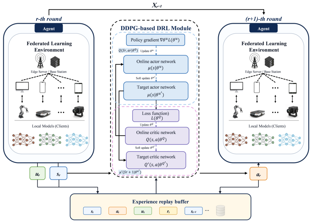
In this section, we introduce the design principles and system framework of the adaptive joint-optimization federated learning algorithm. The system framework is shown in Figure 1 and mainly includes two parts: a federated learning module and a DRL module. The federated learning module mainly includes user-terminal devices and model information, aggregates user model parameters, and outputs a new global model for the next round. The DRL module interacts with the federated learning environment in real time and outputs adaptive decisions. It is mainly responsible for perceiving the training state, dynamically adjusting the parameters of each participating user for the next training round, and updating the neural-network parameters at specific times.

Deep reinforcement learning is an optimization method that obtains feedback from the environment to guide behavior and has clear advantages in fields such as automatic control, robotics, and distributed systems. We first model the adaptive hyperparameter-selection process as a Markov decision process (MDP) suitable for federated learning scenarios to accurately simulate changes in the training state. The Markov decision process is represented by the five-tuple $(\mathcal{S},\mathcal{A},U,P,\beta )$, where $\mathcal{S}$ represents the state set, $\mathcal{A}$ represents the action set, and $\mathrm{U}$ represents the reward function. Each state-action pair $(s_r,a_r)$ yields an immediate reward $u_r=U\left(s_r,a_r\right)$. Here, P is the state-transition probability, indicating the probability of transitioning to a specific state after taking an action in the current state. The discount factor $\beta \in [0,1]$ reflects the decreasing influence of the current reward on future long-term rewards. The main goal of reinforcement learning is to enable the agent to identify appropriate action strategies in different states and maximize the long-term accumulated reward through continuous interaction, namely $u_R={\sum }_{r=1}^R{\beta }^{r-1}{u}_r$. Next, specific definitions are given for the state, action, and reward function of the system considered in this article.

5.1. State Space

At the r-th iteration, the state $s_r$ is composed of the following components:

• The global loss at the r-th iteration: ${\overrightarrow{l}}_r={\displaystyle \frac{{\sum }_{i\in S_r}{l}_r^{\left(i\right)}}{|S_r|}}$, where $l_r^{\left(1\right)},\dots ,l_r^{\left(N\right)}$ correspond to the losses on the local datasets of the users, respectively.
• The global loss at the $(r-1)$-th iteration: ${\overrightarrow{l}}_{r-1}={\displaystyle \frac{{\sum }_{i\in S_{r-1}}{l}_{r-1}^{\left(i\right)}}{|S_{r-1}|}}$.
• The number of local updates at the $(r-1)$-th iteration: ${\tau }_{r-1}$.
• The number of quantization bits at the $(r-1)$-th iteration: $b_{r-1}$.
• The amount of uncompressed information at the $(r-1)$-th iteration: $cn{y}_{r-1}$.
• The compressed communication volume at the $(r-1)$-th iteration: $c{n}_{r-1}$.
• The bandwidth-allocation strategy at the $(r-1)$-th iteration: $B^{r-1}=[B_1^{r-1},\dots ,B_n^{r-1}]$.
• The computational-frequency allocation strategy at the $(r-1)$-th iteration: $g^{r-1}=[g_1^{r-1},\dots ,g_n^{r-1}]$.
• The channel state at the r-th iteration: $h^r=[h_1^r,\dots ,h_n^r]$.

In summary, the state at the r-th iteration is

$$\begin{array}{cc}\hfill s_r=& [{\overline{l}}_r,{\overline{l}}_{r-1},{\tau }_{r-1},b_{r-1},cn{y}_{r-1},c{n}_{r-1},\hfill \\ \hfill & B_1^{r-1},\dots ,B_n^{r-1},g_1^{r-1},\dots ,g_n^{r-1},h_1^r,\dots ,h_n^r].\hfill \end{array}$$

(19)

5.2. Action Space

At the r-th iteration, the action $a_r$ is composed of the following components:

• The change in the number of local updates at the r-th iteration: ${\tau }_r$.
• The change in the number of quantization bits at the r-th iteration: $b_r$, which is mapped to the corresponding quantization level ${\gamma }_r$ according to (8).
• The bandwidth-allocation strategy at the r-th iteration: $B^r=[B_1^r,\dots ,B_n^r]$.
• The computational-frequency allocation strategy at the r-th iteration: $g^r=[g_1^r,\dots ,g_n^r]$.

In summary, the action at the r-th iteration is

$$a_r=\left[{\tau }_r,b_r,B_1^r,\dots ,B_n^r,g_1^r,\dots ,g_n^r\right].$$

(20)

Note that the two discrete variables, i.e., the number of local updates ${\tau }_r$ and the quantization bits $b_r$, are scaled to the respective integer ranges and rounded to the nearest integer using nearest-neighbor rounding. For the continuous variables, $B_n^r$ is projected to simplex via Softmax, and $g_n^r$ is mapped to $[0,g^{\max }]$ via Sigmoid to satisfy the constraints in (18). We adopt the n-way k-shot setting from few-shot learning to simulate heterogeneous data distributions. For each client i, we first draw a base number of classes $n_i\sim \mathrm{Uniform}(\overline{n}-\rho ,\overline{n}+\rho )$, where $\overline{n}$ is the average number of classes per client. $\rho \in \{2,3,5\}$ controls the degree of class-space heterogeneity. We define $\rho$ as the maximum deviation from the mean in both the number of classes and the number of samples per class. A larger $\rho$ leads to greater diversity in both the class space and the data size per class, thus creating a more heterogeneous overall data distribution. For each selected class c of client i, we draw a per-class sample count $k_{i,c}\sim \mathrm{Uniform}(\overline{k}-\rho ,\overline{k}+\rho )$, where $\overline{k}$ is the average number of samples per class. The total number of samples per client is fixed. The client partition is fixed and reused consistently across all experiments. The dataset is randomly partitioned into 80% training and 20% testing samples per client.

5.3. Reward Function

The entire DRL-network training process is guided by rewards. After the parameter server in state $s_r$ executes the parameter-selection strategy specified by action $a_r$, it receives feedback at the end of the training round that evaluates the contribution of this action to the optimization objective; this feedback is called the reward. We denote the reward received at the end of each FL training round by $R_r$. The reward must be carefully designed to minimize the system cost and enable the RL model to help the FL system converge with the highest possible communication efficiency. It is defined as follows:

$$R_r=-\left[{\displaystyle \frac{AE\left(T_r\right)}{T\tau }}+{\displaystyle \frac{L^2{\alpha }^2(\tau -1)(2\tau -1)}{6}}+{\displaystyle \frac{Ld{\alpha }^2\tau }{M{\gamma }^2}}+{\displaystyle \frac{L}{M}}\left(1+{\displaystyle \frac{M-1}{N-1}}\right){\alpha }^2\right].$$

(21)

where constant $A>0$ is a scaling factor introduced to balance the numerical magnitudes between the time-related term and the accuracy-related term in the upper bound.

There are many training algorithms for selecting the optimal action, including value-based and policy-based learning [37]. DDPG is a policy-based deep reinforcement learning method that represents the deterministic policy $\mu \left(s\right)$ using a deep neural network and updates the network parameters using the deterministic policy gradient. It is suitable for reinforcement learning scenarios with large or continuous action spaces. The DDPG training process is shown in Algorithm 1.

Algorithm 1 The Proposed DDPG-Based Resource-Optimization Algorithm

Require: global model ${\overline{x}}_0$, number of user nodes N, number of selected users M, reward discount factor $\beta$, critic network Q, actor network $\mu$, corresponding target networks $Q^{\prime }$ and ${\mu }^{\prime }$, target-network reset interval $step$, maximum local epochs ${\tau }_{\max }$, maximum quantization bits $b_{\max }$, replay buffer size $B_{\mathrm{size}}$, number of episodes E, number of communication rounds per episode R

Ensure: global model ${\overline{x}}_R$

1: Randomly initialize ${\theta }^Q$ and ${\theta }^{\mu }$; set ${\theta }^{Q^{\prime }}\leftarrow {\theta }^Q$, ${\theta }^{{\mu }^{\prime }}\leftarrow {\theta }^{\mu }$  2: Initialize experience replay buffer D with capacity $B_{\mathrm{size}}$  3: Server-side:  4: for $e=1$ to E do  5:    Initialize the global model as ${\overline{x}}_0$  6:    $tmp=0$  7:    for $r=0$ to $R-1$ do  8:      Randomly select $\left|S_r\right|=M$ users from the user set  9:      Send the global model ${\overline{x}}_r$ to the selected users 10:     Receive the loss values from the user nodes 11:     Update the state $s_r$ 12:     Input $s_r$ into the $DDPG$ module to obtain action $a_r$ and the corresponding ${\gamma }_r,{\tau }_r,B_n^r,g_n^r$ 13:      Send ${\tau }_r,b_r,B_n^r,g_n^r$ to all selected users 14:      for each selected user $i\in S_r$ in parallel do 15:           $Y_{\gamma }\left({\Delta }_r^{\left(i\right)}\right)\leftarrow ClientUpdate(i,{\overline{x}}_r,b_r,{\tau }_r,B_n^r,g_n^r)$ 16:      end for 17:      Update the global model to ${\overline{x}}_{r+1}$ according to (10) 18:      Calculate the reward $R_{r-1}$ according to (21) 19:      Store $\left(s_{r-1},a_{r-1},R_r,s_r\right)$ in the experience replay buffer D 20:      Sample experience from D to update the critic network and actor policy network 21: $$ 22:      if $tmp\mathrm{mod}step=0$ then 23:                     ${\theta }^{Q^{\prime }}\leftarrow \tau {\theta }^Q+(1-\tau ){\theta }^{Q^{\prime }}$ 24:                     ${\theta }^{{\mu }^{\prime }}\leftarrow \tau {\theta }^{\mu }+(1-\tau ){\theta }^{{\mu }^{\prime }}$ 25:      end if 26:      $tmp+=1$ 27:     end for 28: end for 29: return the final global model ${\overline{x}}_R$ 30: ClientUpdate($i,{\overline{x}}_r,{\tau }_r,b_r,B_n^r,g_n^r$): 31: Initialize model $x_{r,0}^{\left(i\right)}={\overline{x}}_r$ 32: for $k=1$ to ${\tau }_r$ do 33:     Update the local model as (3) 34: end for 35: Calculate the gradient accumulator ${\Delta }_r^{\left(i\right)}$ according to (5) 36: Parameter quantization is performed according to (6), and the quantization level is $2^{b_r}$

6. Performance Evaluation

To verify the effectiveness of the algorithm, we set the number of participating users N to 13 and select 10 users in each round during training. The experimental environment and parameter settings are summarized in

Table 1. Configuration of the Execution Environment.

Network Structure	Parameter Information
CPU	12th Gen Intel(R) Core(TM) i5-12400F 2.50 GHz
GPU	NVIDIA GeForce GTX 3070
OS	Win 10
Deep learning framework	torch 1.13.0 + cu117
Editor	Pycharm Community 2023.3

and

Table 2. Training hyperparameter settings.

Parameter	Setting
ResNet learning rate	0.001
ResNet batch size	32
DDPG actor learning rate	$1\times {10}^{-4}$
DDPG critic learning rate	$1\times {10}^{-3}$
DDPG mini-batch size	10

, respectively. We selected the widely used NEU-DET dataset [38], which contains a total of 1800 samples, for the experiments.

The standard torchvision ResNet-18 architecture is adopted and initialized from scratch, with its original classification layer replaced by a 512–ReLU–6 head. All images are converted to RGB, resized to $224\times 224$, transformed into tensors, and normalized using a channel-wise mean and standard deviation of $(0.5, 0.5, 0.5)$, without additional data augmentation. The DDPG actor adopts a 48–400–300–22 architecture with LayerNorm and ReLU activations in the hidden layers and a tanh output layer, whereas the critic adopts a 70–400–300–1 architecture with ReLU activations. Exploration is performed by adding Gaussian noise $\mathcal{N}(0, 0.{15}^2)$ to each action component, followed by clipping to $[-1, 1]$. The replay-buffer capacity is 10,000 transitions. The target networks are soft-updated after each DDPG update with a coefficient of $\zeta =0.001$, and the discount factor is set to $\beta =0.99$. For each random seed, the DDPG controller is trained online for one episode consisting of 20 federated communication rounds, and five independent random seeds are evaluated.

To simulate Non-IID (non-independent and identically distributed) data, we introduce n to control the number of classes and k to control the number of instances in each class, following [39]. To investigate the impact of Non-IID data on training performance, we set three levels of dataset heterogeneity across clients. We adopt the concept of n-way k-shot learning from few-shot learning, where n controls the number of classes and k controls the number of training instances in each class. To simulate heterogeneous scenarios, we randomly vary the values of n and k across devices. We first define the average values of n and k and then add random noise to each user’s n and k. The variance of n controls the heterogeneity of the class space, whereas the variance of k controls the imbalance in data size. We define $\rho$ to balance n and k. As $\rho$ increases, the client class distributions and data sizes become more diverse, resulting in greater dataset heterogeneity. For the main $\rho \left(2\right)$ setting, each participating client contains 108 training images. The actual partition gives an average of $\overline{n}=2.2$ observed classes per client and an effective average of $\overline{k}=50.4$ samples per class. The client partition is fixed across all methods, and five independent training seeds (1–5) are used. Therefore, the main Non-IID setting mainly reflects label-distribution heterogeneity rather than client-level sample-size imbalance.

6.1. Simulation of Local Training Frequency and the Quantization Mechanism

To verify the effectiveness of the proposed algorithm, we compare it with three other algorithms under different settings of $\gamma$ and $\tau$. Because the reward functions of the comparison algorithms cannot directly use our proposed reward function, we set their reward function to $R_r=-\left|l_r-{\overline{l}}_{r-1}\right|-\left({\displaystyle \frac{T_r}{C}}\right)$, where C is a constant. The initial number of local updates for the proposed algorithm is 1, the quantization level is $2^{16}$, and the computation-frequency range is 200–400 MHz. To explore the impact of data heterogeneity on algorithm performance, all algorithms are tested under three data-distribution settings, with identical initial computation-frequency and bandwidth-allocation settings. The goal of the proposed algorithm is to maintain high communication efficiency while accelerating convergence, that is, to minimize the training loss in each communication round. Therefore, curves with respect to the number of communication rounds are plotted.

• AdaQuantFL: This is an advanced adaptive compression algorithm that can explicitly calculate the quantization level from loss values. However, it does not consider the impact of the local update frequency.
• Local: The number of local updates $\tau$ is set to 5, which is a median value, and the quantization level $\gamma$ is set to $2^8$.
• Pone: The participating devices perform only one local update in each training round. This method minimizes the impact of model differences among users. The quantization level $\gamma$ is set to $2^8$, which is also a median value.

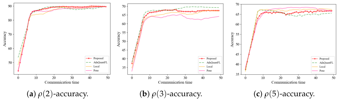
Figure 2 shows the image-classification results obtained using ResNet for datasets with different levels of Non-IID data. The horizontal axis represents the communication round, and the vertical axis represents the test accuracy. The results show that the test accuracy increases as training progresses and stabilizes after a certain number of communication rounds, verifying the effectiveness of the proposed algorithm. In Figure 2a, the Non-IID degree is $\rho \left(2\right)$. The test accuracies of the proposed and comparison algorithms are close, although the proposed algorithm performs slightly better. In Figure 2b, the Non-IID degree is $\rho \left(3\right)$. After 50 communication rounds, the proposed algorithm is slightly inferior to AdaQuantFL in terms of test accuracy but outperforms Local and Pone. The reason is that the proposed algorithm uses a high quantization level in the later stage, which causes greater precision loss. In Figure 2c, the Non-IID degree is $\rho \left(5\right)$. There is little difference among the algorithm curves after convergence. Pone is not optimal at the beginning but achieves the best performance in the middle stage before declining slightly. Local and AdaQuantFL perform best initially, but the accuracy of AdaQuantFL declines in the later stage. The proposed algorithm is inferior to Local in the early stage because it performs fewer local updates than Local, and it is inferior to Pone in the middle stage because of its higher quantization level; however, its accuracy increases again as the number of communication rounds increases. Pone allows each device to perform only one local update, which slows the improvement in accuracy. However, Pone uses as few local updates as possible to minimize model differences among devices. Consequently, its test accuracy eventually reaches the optimal level but declines at the end, indicating that an excessive communication frequency is unnecessary.

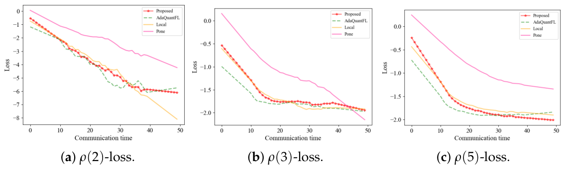
The horizontal axis in Figure 3 represents the number of communication rounds, and the vertical axis represents the training loss. The results show that the training loss decreases as training progresses and stabilizes after a certain number of communication rounds. In Figure 3a, the Non-IID degree is $\rho \left(2\right)$. The training losses of the proposed algorithm and AdaQuantFL decrease more steadily, the training loss of Local decreases more substantially in the later stage, and that of Pone decreases the most slowly. The higher quantization level of the proposed algorithm in the later stage slows the decrease in training loss. In Figure 3b, the Non-IID degree is $\rho \left(3\right)$. The training losses of the proposed algorithm, Local, and AdaQuantFL decrease at similar rates, whereas the training loss of Pone decreases sharply late in training. This result indicates that an appropriate number of local updates can accelerate training-loss convergence compared with excessive reliance on communication. In Figure 3c, the Non-IID degree is $\rho \left(5\right)$. The training losses of the proposed algorithm, Local, and AdaQuantFL decrease at similar rates, consistent with the results in Figure 3b. The only difference is that the training loss of Pone remains higher than those of the other three algorithms.

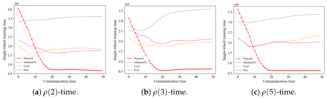
The horizontal axis of each plot in Figure 4 represents the number of communication rounds, and the vertical axis represents time. The results show that the time stabilizes as training progresses. Figure 4 shows similar trends under the three settings, and the proposed algorithm demonstrates a substantial advantage in terms of time. AdaQuantFL consumes the most time, whereas Local and Pone perform similarly. The reason is that all algorithms use the same computation-frequency selection and bandwidth-allocation strategies; therefore, the differences arise from their differences.

As the degree of Non-IID data across devices increases from $\rho \left(2\right)$ to $\rho \left(5\right)$, the algorithm maintains convergence, although the test accuracy decreases. When three classes are assigned to each device, the test accuracy decreases significantly. When five classes are assigned to each device, the performance is similar to that under $\rho \left(3\right)$. Figure 2, Figure 3 and Figure 4 show that the proposed algorithm can effectively reduce the training loss and maintain a small difference in test accuracy while achieving the minimum time cost compared with the other algorithms. In other words, the proposed algorithm achieves the minimum error in the shortest time. Compared with AdaQuantFL, the proposed algorithm achieves faster loss convergence by controlling four variables. Local and Pone use fixed numbers of local updates and quantization levels. The difference between Local and Pone lies in their numbers of local updates. This difference is not obvious in terms of time; however, in terms of training loss, Pone clearly decreases more slowly.

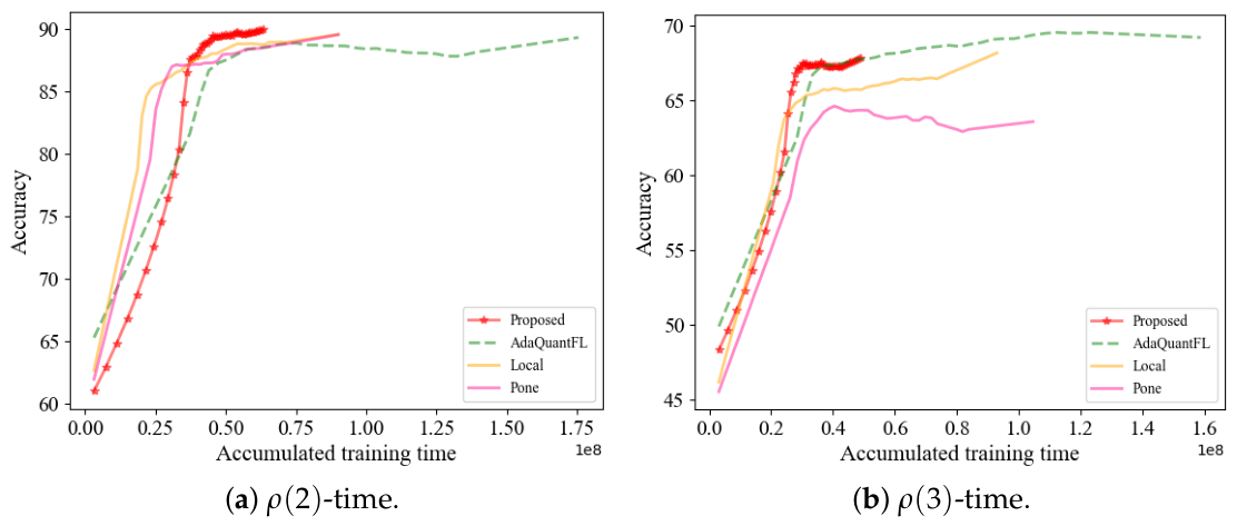
Time is used as the horizontal axis, whereas accuracy and training loss are used as the respective vertical axes to compare the proposed and comparison algorithms under $\rho \left(2\right)$ and $\rho \left(3\right)$, as shown in Figure 5. The proposed algorithm achieves the highest accuracy in the shortest time under both $\rho \left(2\right)$ and $\rho \left(3\right)$, further demonstrating its advantages.

6.2. Simulation of Resource Scheduling

The goal of this chapter remains to minimize the training loss in each round under a given time limit. As shown in the previous experiments, as the Non-IID degree of the data increases, the proposed algorithm adaptively adjusts the number of local updates and the quantization level. Although it is slightly inferior in test accuracy, it has a clear advantage in terms of time. To further investigate the impact of bandwidth allocation and computation-frequency selection on the proposed algorithm, we introduce the following four comparison algorithms. Except for their bandwidth-allocation and computation-frequency selection strategies, these comparison algorithms use the method proposed in this chapter to jointly regulate the number of local updates and the quantization level:

• Fixed Bandwidth Allocation, Optimized Local Computing Capacity (OCA): The computation frequency of the defect-detection equipment is set to 400 MHz, while bandwidth allocation follows the proposed algorithm.
• Fixed Local Computing Capacity, Optimized Bandwidth Allocation (OBA): The bandwidth is equally allocated among the defect-detection devices, while computation-frequency allocation follows the proposed algorithm.
• Equal Client (EC): The bandwidth is equally allocated among the devices, and the computing frequency of each edge device is set to 400 MHz.
• Random Allocation (Random): The computation frequency of each edge device is randomly selected from $[200, 400]$ MHz, and the bandwidth is randomly allocated among the devices.

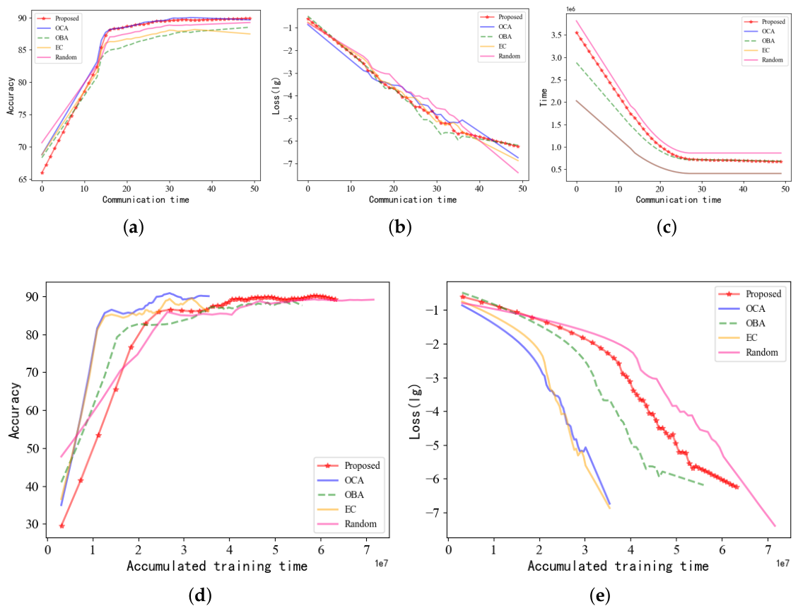
Experiments are conducted under the $\rho \left(2\right)$ setting, and the results are shown in the following figure.

Figure 6a shows how the test accuracies of the proposed and comparison algorithms change as the number of communication rounds increases. The proposed algorithm and OCA exhibit comparable performance and outperform the other comparison algorithms. Figure 6b shows how the training losses of the proposed and comparison algorithms change as the number of communication rounds increases. The performance of the proposed algorithm is close to that of EC. Figure 6c shows how the times of the proposed and comparison algorithms change as the number of communication rounds increases. OCA and EC outperform the proposed algorithm, while the proposed algorithm outperforms Random. As the number of communication rounds increases, the performance of the proposed algorithm catches up with that of OBA. Figure 6d shows how the test accuracies of the proposed and comparison algorithms change over time. EC and OCA achieve high test accuracy in a relatively short time, and the proposed algorithm also achieves satisfactory test accuracy after a period of time, outperforming OBA and Random. Figure 6e shows how the training losses of the proposed and comparison algorithms change over time. EC and OCA perform similarly to, and better than, OBA, the proposed algorithm, and Random.

In summary, OCA and EC perform well, with EC representing the ideal case. OCA sets the computation frequency to its maximum value. The proposed algorithm catches up with EC and OCA, performs on par with OBA, and outperforms Random. These results demonstrate the effectiveness of the proposed algorithm. The proposed algorithm is advantageous because it jointly controls computation-frequency selection and bandwidth allocation through reinforcement learning.

7. Conclusions

This paper proposed an adaptive federated learning framework that jointly optimizes the local update frequency, gradient quantization level, bandwidth allocation, and computing-resource allocation for heterogeneous industrial Internet of Things devices. A convergence upper bound was first derived to characterize the effects of these variables on model error and training time. The joint optimization was then formulated as a Markov decision process and solved using a DDPG-based algorithm. Experiments on the NEU-DET dataset under different Non-IID settings showed that the proposed method maintains competitive classification accuracy while reducing training time. The resource-scheduling results further demonstrated the benefit of jointly adapting communication and computing resources compared with fixed or random allocation strategies. Additionally, we will also explore the integration of energy-aware optimization into the current framework, particularly for battery-constrained IIoT devices.