Individual and Coordinated Mixed-Integer Linear Programming Dispatch of an Industrial Photovoltaic–Battery Prosumer Community on the Bulgarian Day-Ahead Market

Abstract

Industrial consumers increasingly operate photovoltaic (PV) generation and battery energy storage systems (BESS) against volatile day-ahead electricity prices. This paper presents a simulation environment for a community of three heterogeneous industrial prosumers, anchored in twelve months of day-ahead prices from the Bulgarian Independent Energy Exchange (IBEX), commercial hardware envelopes, and the terms of a market offtake contract that indexes remuneration to the day-ahead price, passes negative prices through to the producer, and mandates curtailment in strongly negative periods. A mixed-integer linear programming (MILP) dispatch model with binary charge/discharge modes and endogenous PV curtailment is solved daily in independent and coordinated regimes, under cost-only and capacity-aware objectives, for Sofia and Stara Zagora. On an energy-only basis, before capacity charges, storage turns the community from a net payer (39.1 kEUR/yr grid-only; 13.1 kEUR/yr with PV) into a net earner (8.64 kEUR/yr independent; 10.12 kEUR/yr coordinated), and the battery retrofit more than doubles the merchant plant’s net revenue. Cost-optimal dispatch synchronizes charging and raises the coincident grid peak to 241 kW; a capacity-aware objective cuts it to 133–140 kW (−42–45%) for under 0.9 kEUR/yr foregone income; under the two tested capacity-charge conventions, only the capacity-aware schedule remains net-positive after the modeled charge. The coordination gain grows with the import price adder and remains positive across 15–45 EUR/MWh.

1. Introduction

The decarbonization of the power sector and the rapid uptake of distributed photovoltaic (PV) generation have reshaped the role of electricity consumers. Industrial and commercial sites that once behaved as passive loads increasingly host on-site PV and battery energy storage systems (BESS), turning them into prosumers that both consume and inject energy, while dedicated small merchant PV plants sell their entire output on the market. At the same time, wholesale electricity is settled on day-ahead markets whose prices are highly volatile and, with growing renewable penetration, frequently fall to zero or negative values. The economic value that a prosumer can extract from its assets therefore depends critically on how PV self-consumption, storage dispatch, and—increasingly—production curtailment are scheduled against these price signals.

This shift is explicitly targeted by national and European policy. Directive (EU) 2023/2413 (RED III) raises the binding renewable share and promotes self-consumption and renewable energy communities, while the European Green Deal and the Digital Europe agenda emphasize digital tools—including simulation and digital twins—for managing decentralized energy systems [1,2]. In Bulgaria, the day-ahead market operated by the Independent Bulgarian Energy Exchange (IBEX) moved to 15 min settlement in late 2025, and offtake contracts for small producers are now routinely indexed to the day-ahead clearing price, exposing producers directly to market volatility, negative prices, and curtailment obligations.

Most prior techno-economic studies of prosumer storage focus on a single residential site, use synthetic or short price windows, assume stylized feed-in remuneration, and evaluate rule-based controllers. Comparatively little attention has been paid to (i) industrial prosumers and merchant PV plants dispatched against a full year of real day-ahead prices from a specific market, (ii) remuneration modeled on the terms of an actual offtake contract, including administrative fees, negative-price exposure, and mandatory curtailment, (iii) the difference between independent and coordinated operation of several heterogeneous sites forming an energy community, and (iv) the grid-side effects of cost-optimal scheduling and how to correct them within the same optimization framework.

This paper addresses these gaps through a reproducible simulation environment built entirely on real Bulgarian market data, real commercial equipment envelopes, and a real contractual framework.

The optimization machinery employed here is deliberately standard; the contribution lies in what that machinery is anchored to. The contributions of this work are fivefold. First, we build a year-long, hourly simulation environment for a community of three heterogeneous industrial prosumers using twelve months of real IBEX day-ahead prices, spanning the market’s transition from hourly to 15 min settlement. Second, we anchor the export side in a real market offtake contract—remuneration at the day-ahead price minus a fixed 2.15 EUR/MWh administrative fee, negative-price exposure, and a stop-production obligation—and represent curtailment endogenously in the optimization. Third, we formulate a MILP dispatch model with binary charge/discharge modes and solve it in independent and coordinated regimes, quantifying the value of local energy sharing for a community that includes a real 98.56 kWp merchant PV plant retrofitted with a 261 kWh battery. Fourth, we show that cost-optimal dispatch concentrates imports in the cheapest hours and inflates the coincident grid peak, and that a capacity-aware objective removes this side effect for less than 0.9 kEUR/yr of foregone income. Fifth, we compare two locations—Sofia and Stara Zagora—to quantify the sensitivity of all indicators to the solar resource.

The remainder of the paper is organized as follows. Section 2 reviews related work. Section 3 describes the community, the hardware, the market data and contractual framework, the optimization model, and the evaluation indicators. Section 4 presents the results, Section 5 discusses their implications and limitations, and Section 6 concludes.

2. Related Work

Prosumer energy management has been studied extensively for residential systems, where rule-based and optimization-based controllers schedule PV and storage to maximize self-consumption or minimize cost; Luthander et al. provide a widely cited review of PV self-consumption in buildings [3]. Optimization approaches based on (mixed-integer) linear programming are broadly adopted because they handle storage dynamics, power and energy limits, and time-varying tariffs within a tractable formulation, and they serve as the standard benchmark against which learning-based controllers are evaluated [4]. Studies of commercial and industrial storage add demand-charge management and peak-aware scheduling [5], but typically assume stylized export remuneration rather than the terms of an actual offtake contract.

A second body of work addresses energy communities and peer-to-peer energy sharing, in which several prosumers coordinate to increase collective self-consumption, reduce community import, or provide flexibility services [6,7]. Coordination is generally found to improve aggregate indicators, although the magnitude depends strongly on tariff structure and on the diversity of the participating load and generation profiles. The spread between import and export prices—in our setting, a network-and-supply adder on imports versus an administrative fee on exports—determines the direct monetary value of internal sharing, a dependence that we quantify explicitly on a real contract.

With rising renewable penetration, negative day-ahead prices and producer curtailment have moved from curiosities to routine operating conditions on European markets. Offtake contracts increasingly pass negative prices through to producers and impose stop-production obligations during strongly negative periods, which makes endogenous curtailment a first-class decision variable in dispatch optimization rather than an afterthought. Few community-level studies represent this contractual mechanism explicitly; doing so is one of the distinguishing features of the present model.

Recent studies confirm the growing economic weight of these mechanisms and of coordinated operation. Mercier et al. [8] quantify the arbitrage value of storage on day-ahead markets across Europe with a MILP formulation and show that network fees can erode 20–50% of it; Prokhorov and Dreisbach [9] link rising renewable penetration to the increasing incidence of negative spot prices; Aranzabal et al. [10] develop optimal community management for PV–battery prosumers across energy and ancillary-service markets; and Fotopoulou et al. [11] optimize the day-ahead operating cost of energy communities with explicit cost allocation among members. Capacity-based network charging, which motivates our peak-aware objective, is an established element of European distribution tariff design [12]. Against this background, the present study differs in anchoring dispatch to the full terms of a real Bulgarian offtake contract—including negative-price pass-through and mandatory curtailment—for an industrial community that contains a real merchant plant.

Finally, the digital-twin paradigm frames such models as active, data-synchronized virtual replicas of physical energy systems rather than static simulations [13]. This perspective motivates building the prosumer model around real measured market data, real equipment envelopes, and real contractual terms, so that the environment can later be coupled to live data streams from the physical sites. The present work sits at the intersection of these strands. Its novelty lies not in the MILP formulation itself—which is deliberately standard and well understood—but in the contract-anchored integration: negative-price pass-through and endogenous curtailment taken from an actual offtake contract, twelve months of real IBEX prices spanning the market’s hourly-to-15 min transition, commercial BESS envelopes that bound the dispatch, and individual versus coordinated operation of a heterogeneous industrial community that includes a real merchant PV plant. To the best of our knowledge, no prior study combines these elements on the Bulgarian market.

3. Materials and Methods

3.1. Community and Hardware

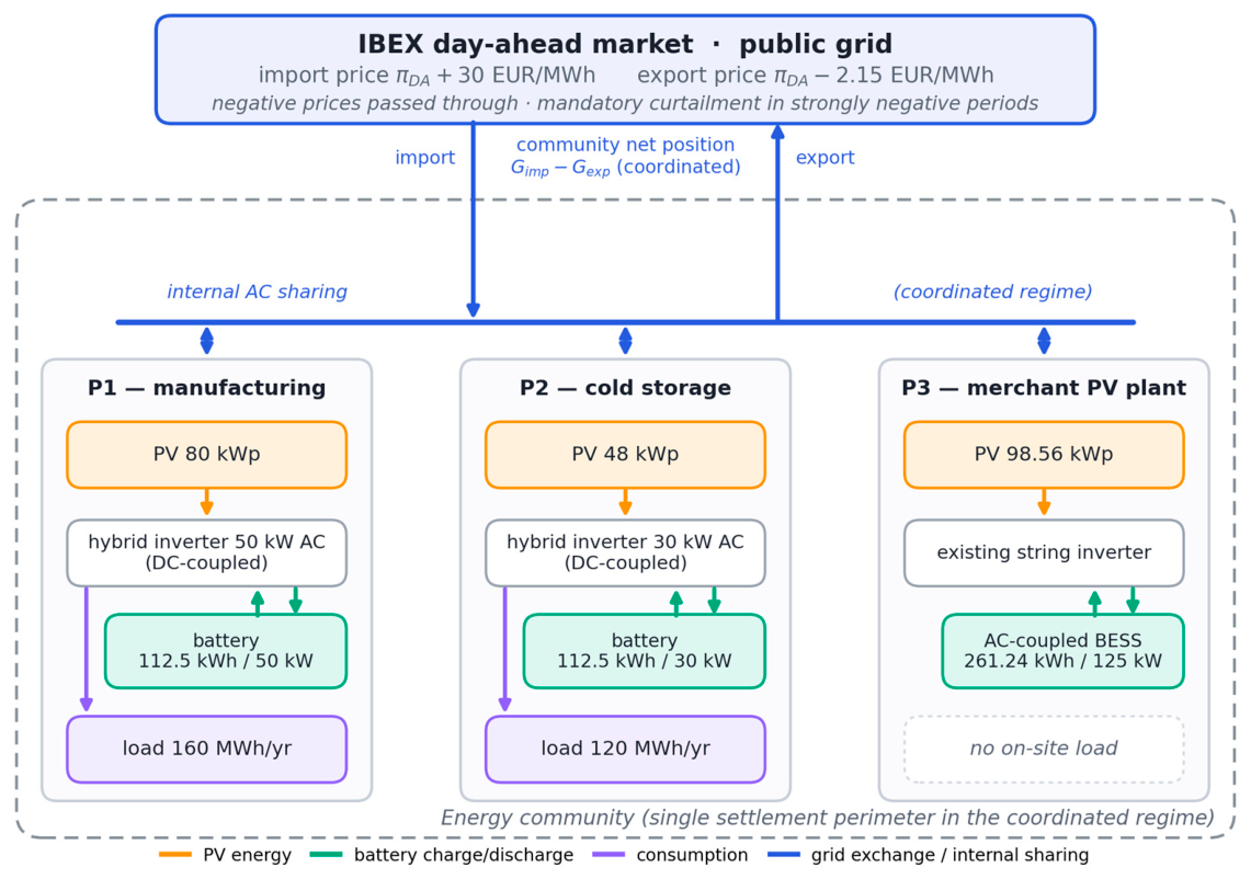
We consider a local energy community of three grid-connected industrial sites (P1–P3) with heterogeneous roles, load profiles, PV arrays and storage systems, all based on commercially available Suntech SunStorage PRO equipment (Suntech, Wuxi, China). Two distinct integration architectures are represented, reflecting the two dominant retrofit paths in practice. The overall architecture—the three sites with their PV, storage and load subsystems, the internal sharing of the coordinated regime, and the market interface with its contractual price terms—is shown schematically in Figure 1.

P1 and P2 are producing consumers: industrial sites with on-site loads that generate, consume, and sell surplus energy. Both use the DC-coupled hybrid architecture of the modular SunStorage PRO storage family [14]: P1 combines the Suntech SunStorage PRO STE-50HT-150 hybrid inverter (50 kW AC output, recommended PV input up to 80 kWp) with the SunStorage PRO STE-112A-DC LiFePO4 cabinet (112.5 kWh, 314 Ah cells, 90% depth of discharge, rated at 8000 cycles, battery charge/discharge efficiency of 97.5% per direction, i.e., approximately 95% round-trip); P2 uses the smaller SunStorage PRO STE-30HT-150 inverter (30 kW AC, up to 48 kWp PV) with an identical STE-112A-DC cabinet. The hybrid inverter couples PV and battery on the DC side and imposes a hard AC output limit, which our model represents explicitly.

P3 is a real merchant PV plant: a 98.56 kWp installation in southern Bulgaria (EVN distribution area) that sells its entire output on the market through an offtake contract and has no significant on-site load. The plant retains its existing string inverter; storage is retrofitted with the AC-coupled Suntech SunStorage PRO STE-261L-125P all-in-one cabinet [15]: 261.24 kWh of LiFePO4 capacity (LFP 314 Ah cells), 125 kW rated power conversion, 95% depth of discharge, ≥8000 cycles, and a system round-trip efficiency of ≥89% including the integrated power conversion stage. Because the cabinet contains no PV inverter, it attaches at the plant’s AC bus—precisely the configuration assumed here, in which existing PV assets are upgraded with storage without replacing the PV inverter. Export at each site is bounded by its connection capacity, taken equal to the installed AC rating.

Table 1. Prosumer community configuration. P1 and P2 are DC-coupled hybrid systems behind industrial loads; P3 is a real merchant PV plant retrofitted with an AC-coupled all-in-one BESS. State-of-charge windows are 10–100% (P1, P2) and 5–100% (P3), consistent with the respective depth-of-discharge ratings.

Site	Equipment	PV (kWp)	Battery	Round-Trip/DoD	Load (MWh/yr)
P1 (manufacturing)	Suntech SunStorage PRO STE-50HT-150 + STE-112A-DC	80	112.5 kWh/50 kW	95%/90%	160
P2 (cold storage)	Suntech SunStorage PRO STE-30HT-150 + STE-112A-DC	48	112.5 kWh/30 kW	95%/90%	120
P3 (merchant PV plant)	Existing inverter + Suntech SunStorage PRO STE-261L-125P (AC-coupled)	98.56	261.24 kWh/125 kW	89%/95%	—

summarizes the configuration.

3.2. Market Data and Contractual Framework

Electricity prices are taken from the day-ahead market of the Independent Bulgarian Energy Exchange (IBEX) [16]. We use the trailing twelve months of available data (6 June 2025 to 5 June 2026, 8760 hourly steps). The market moved from hourly to 15 min market time units on delivery day 1 October 2025 (trading day 30 September 2025), with the transition implemented simultaneously across the European Single Day-Ahead Coupling [17]; quarter-hourly prices are accordingly averaged to hourly resolution. Bulgaria adopted the euro on 1 January 2026 at the irrevocably fixed conversion rate of 1 EUR = 1.95583 BGN [18]; prices published in BGN before euro adoption are converted at this rate, while prices already published in EUR are used directly, yielding a continuous hourly series. The compiled and harmonized dataset used in all experiments is openly available [19]. Over this window, the mean price is 115.0 EUR/MWh, with a minimum of −79.5 EUR/MWh, a maximum of 936.7 EUR/MWh, and 191 h of negative prices.

The export side is modeled on the terms of a real market offtake contract with a licensed electricity trader acting as balancing-group coordinator under the national Electricity Trading Rules [20], of the type now standard for small producers on the Bulgarian market. Produced net active energy is purchased at an indexed price equal to the day-ahead clearing price of the relevant settlement period minus a fixed administrative fee of 2.15 EUR/MWh. Crucially, the contract passes negative prices through to the producer—when the clearing price is negative, the producer pays for injected energy—and obliges the producer to stop production in settlement periods notified as strongly negative. We represent this mechanism endogenously: PV output is a decision variable bounded by the available resource, so the optimizer curtails whenever injection would be value-destroying, i.e., whenever the day-ahead price falls below the 2.15 EUR/MWh fee; this encompasses both the mandatory stop-production obligation in strongly negative periods and voluntary economic curtailment at low positive prices.

We further assume that the metering and contractual arrangement permit the batteries to charge from the grid and that all exported energy is settled at the contract price; where contract terms or guarantees of origin restrict the re-export of grid-charged energy, an additional constraint separating PV-charged from grid-charged energy would be required; the impact of disallowing grid charging is quantified in Section 4.9. Balancing costs, which the contract allocates to the producer within a standard balancing group, are outside the scope of the day-ahead dispatch model and are noted as a limitation. On the consumption side, imports are priced at the day-ahead price plus a network-and-supply adder of 30 EUR/MWh, a representative assumption for industrial supply contracts.

3.3. PV Resource and Load Modeling

PV generation is modeled physically for a south-facing (azimuth 0°) array tilted at 35°. Hourly plane-of-array irradiance is computed from solar geometry and an atmospheric transmittance, scaled by a monthly clearness index and a performance ratio of 0.82, and clipped at the AC rating of the respective inverter. Two locations are evaluated: Sofia (42.70° N), calibrated to a specific annual yield of 1300 kWh/kWp, and Stara Zagora (42.43° N) in the sunnier south—the region where the real P3 plant operates—calibrated to 1390 kWh/kWp; both values are consistent with estimates from the European Commission’s PVGIS tool for these locations [21]. Load profiles for P1 and P2 are representative synthetic time series for the two industrial archetypes (single-shift manufacturing with a daytime peak, and continuous cold storage with a flat profile and a mild night dip), with weekday/weekend modulation, scaled to the annual energies in Table 1; they are intended to be replaced by metered data as the sites are instrumented. P3 carries no load, reflecting the real plant. Specifically, the normalized hourly shape of P1 is s₁(h) = 0.25 + 0.75·max{sin(π(h − 6)/12), 0} with a weekend factor of 0.40 (single-shift manufacturing), and that of P2 is s₂(h) = 0.85 + 0.15 ·cos(π(h − 15)/12) with a weekend factor of 0.92 (continuous cold storage); both shapes are normalized so that the annual energies match Table 1. The sensitivity of the results to these synthetic shapes is tested with alternative industrial profiles in Section 4.9.

3.4. MILP Dispatch Model

Each site is modeled at its AC node with the following hourly variables over a time step Δt = 1 h: grid import g_imp and export g_exp, battery charge p_ch and discharge p_dis, dispatched PV output g_pv (curtailment allowed), stored energy e_t, and a binary mode indicator y_t ∈ {0,1} that forbids simultaneous charging and discharging. Given the day-ahead load L_t and the available PV resource ĝ_pv, the daily cost-minimization problem for one site is:

$$min{\sum }_t\left(g_{imp,t}{\pi }_{imp,t}-g_{exp,t}{\pi }_{exp,t}\right)\Delta t-e_T{\pi }_{avg}$$

(1)

where the import and export prices follow the supply assumption and the offtake contract, respectively:

$${\pi }_{imp,t}={\pi }_{DA,t}+f_{imp},\hspace{1em}\hspace{1em}{\pi }_{exp,t}={\pi }_{DA,t}-f_{adm},$$

(2)

with f_imp = 30 EUR/MWh and f_adm = 2.15 EUR/MWh. Note that π_exp becomes negative whenever the day-ahead price falls below the administrative fee, so injection is then penalized rather than remunerated—the contractual negative-price pass-through. The constraints are:

$$e_t=e_{t-1}+{\eta }_c{p}_{ch,t}\Delta t-{\displaystyle \frac{p_{dis,t}\Delta t}{{\eta }_d}},$$

(3)

$$L_t+p_{ch,t}+g_{exp,t}=g_{pv,t}+p_{dis,t}+g_{imp,t},$$

(4)

$$p_{ch,t}\le P_{bat}{y}_t,\hspace{1em}\hspace{1em}{p}_{dis,t}\le P_{bat}\left(1-y_t\right),$$

(5)

$$0\le g_{pv,t}\le {\widehat{g}}_{pv,t},\hspace{1em}{E}_{min}\le e_t\le E_{max},\hspace{1em}0\le g_{exp,t}\le G_{conn},\hspace{1em}0\le g_{imp,t}\le G_{imp},$$

(6)

$$g_{pv,t}+p_{dis,t}\le P_{inv},$$

(7)

Here η_c and η_d are the charge and discharge efficiencies (η_c = η_d = √η_rt), G_conn is the export connection capacity, and the first condition in (6) makes curtailment an endogenous decision. The import bound in (6) is set to the site’s AC rating plus the battery charging power. Constraint (7) enforces the joint AC output limit of the DC-coupled hybrid inverters at P1 and P2; the AC-coupled battery at P3 has its own power conversion stage and is limited by its rating and the export cap. The two integration architectures thus differ in three respects: (i) at P1 and P2 dispatched PV and battery discharge share the hybrid inverter’s AC stage and jointly compete for its rating through (7), whereas at P3 no joint limit with the PV inverter applies; (ii) conversion losses are lumped into the per-direction efficiencies ηc = ηd = √ηrt, with ηrt = 95% for the DC-coupled cabinets and ηrt = 89% for the AC-coupled system, the lower figure reflecting the additional AC/DC conversion of its integrated power stage; and (iii) grid charging at P3 passes through the cabinet’s own converter, while at P1 and P2 it shares the hybrid inverter within the same AC limit.

The binary constraints (5) make the model a genuine MILP, and their role merits a precise statement. With strictly positive round-trip losses and non-negative prices, simultaneous charging and discharging is never optimal, so the binaries are typically inactive at the optimum and the LP relaxation attains the MILP optimum. The situation changes in degenerate price regimes. When the export price is negative (191 h in our window), the LP relaxation may admit objective-equivalent loss-dissipating charge/discharge cycles even though PV curtailment is available as a free disposal channel; and when the import price itself becomes negative (π_DA < −30 EUR/MWh, 22 h in our window), such simultaneous cycles become strictly profitable, since dissipating imported energy through the round-trip loss is then remunerated. The binary mode constraints exclude both artifacts—the spurious equivalent optima and the strictly profitable energy burning—and likewise remove analogous objective-equivalent degeneracies under the capacity-aware objective introduced below. There is therefore no contradiction with the empirical observation in Section 4.9 that the LP relaxation is tight for the cost-only objective at 15 min resolution: tightness there is a property of the particular price realization, verified ex post against the MILP solution, whereas the binary constraints guarantee physical consistency for any price series, including the negative-price and peak-priced regimes in which the relaxation can fail. Since the daily instances solve in milliseconds, retaining the binaries costs little and removes the need for case-by-case tightness verification.

The final term in (1) assigns a small terminal value to stored energy at the daily mean import price to avoid spurious end-of-horizon discharging; the horizon is one day (24 h), reflecting the day-ahead market, and the state of charge is carried across consecutive days.

In the coordinated regime, the three sites are optimized jointly as an energy community. Only the community net position interacts with the grid, so internal surpluses—including the merchant plant’s output—offset internal deficits before any import or export occurs:

$$G_{imp,t}-G_{exp,t}={\sum }_{p\in P}\left(L_{p,t}+p_{ch,p,t}-g_{pv,p,t}-p_{dis,p,t}\right),$$

(8)

with the per-site constraints (3) and (5)–(7) retained. The objective replaces the per-site grid flows in (1) with the community flows in (8). All instances are solved to proven optimality with the CBC branch-and-bound solver (v2.10) via PuLP (v3.3): a daily single-site instance comprises 168 variables (24 binary) and about 120 constraints, the coordinated instance roughly 550 variables (72 binary) and 360 constraints, and a full annual evaluation (2920 daily MILPs per location) completes in under one minute on a single CPU core (18 ms per instance on average, 0.5 s worst case).

For reproducibility, the remaining dispatch assumptions are stated explicitly. The state of charge is initialized at 50% of capacity on the first simulated day and carried across consecutive days. End-of-day stored energy is valued at the daily mean import price (the terminal term in (1)); Section 4.9 shows that replacing this valuation with a hard end-of-day restoration to 50% changes the annual results by less than 4% and leaves the coordination gain unchanged. Internal sharing in the coordinated regime is a virtual netting of the three AC nodes at the community boundary, Equation (8): battery and inverter losses are borne inside each site, whereas network losses and charges on internally shared energy are not modeled in the base case and are bounded by the wheeling-fee sensitivity of Section 4.9. Finally, the coordination benefit is reported at community level; its allocation among members is a settlement-design choice that can be layered on top of the dispatch—e.g., proportionally to shared volumes or through cooperative-game schemes as in [11]—without altering the optimization itself.

The coordinated regime should be read as an idealized settlement assumption: the three sites are netted within a single perimeter—as in an energy community or aggregator arrangement—and internally shared energy incurs no wheeling or network charges. Realistic settlement frameworks may levy such charges on shared energy, which would reduce the coordination gain proportionally; the sensitivity of the gain to the import price spread (Section 4.1) and to an explicit wheeling fee on shared energy (Section 4.9) bounds this effect. Whether virtual netting of separately metered sites is permitted depends on the applicable regulatory framework [20].

In the Bulgarian context, specifically, the three sites are separately metered grid users with their own supply and offtake contracts. Since 3 February 2026, the national Electricity Trading Rules [20] have included a dedicated framework for shared electricity involving groups of active customers, citizen energy communities and renewable-energy communities—transposing the energy-sharing provisions of RED II and RED III [1]—which regulates the registration of such groups with the network operators, settlement-period metering with remote reading, a two-stage methodology for allocating the shared quantities, their reflection in suppliers’ invoices, and an exemption from transmission-network charges for shared quantities that meet the operator’s connection criteria (State Gazette No. 13 of 3 February 2026). The coordinated regime modeled here should nevertheless be interpreted as an upper-bound settlement case with frictionless community netting: its practical realization depends on eligibility and registration, network topology, the statutory allocation methodology, the contractual arrangements with supplier and offtaker, and the network charges applicable to shared quantities, which our wheeling-fee sensitivity (Section 4.9) captures only in aggregate. The legal possibility of energy sharing thus now exists; what the model idealizes is the absence of the associated frictions and charges.

3.5. Capacity-Aware Objective

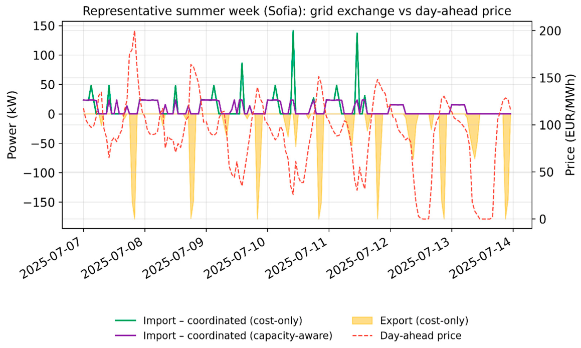
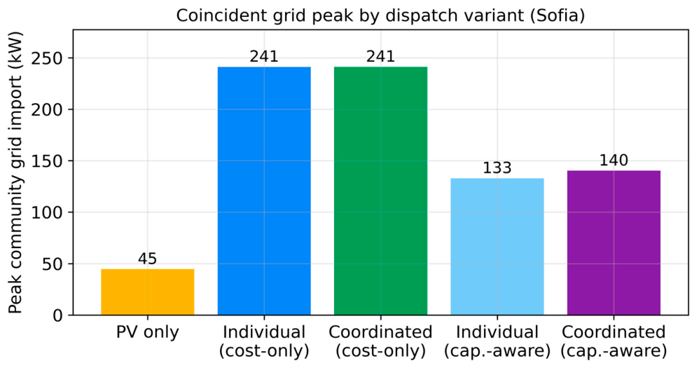
Cost-only dispatch is indifferent to when power is drawn as long as the monetary result is optimal, which concentrates charging in the cheapest hours. To represent connection-capacity limits and demand charges, we extend the objective with a peak term. A daily peak variable p_k bounds the grid import in every hour:

$$p_k\ge g_{imp,t}\hspace{1em}\hspace{1em}\forall t,$$

(9)

and the capacity-aware objective augments the energy cost with the priced peak:

$$min C+c_{cap}{p}_k,$$

(10)

where C denotes the energy-cost objective of (1)—with the community flows of (8) in the coordinated regime, in which case the peak variable bounds the community import G_imp,t instead of the site-level import—and c_cap is the capacity rate.

We use an illustrative capacity-rate parameter of 0.35 EUR/kW per day, rate-equivalent to approximately 10.6 EUR/kW per month. Capacity-based per-kW components are a standard element of European distribution-tariff design [12]; the numerical rate used here is a scenario parameter and is not intended to reproduce a specific regulated tariff. The daily peak penalty is likewise a modeling proxy; Section 4.5 therefore prices the resulting schedules ex post under both daily and equivalent monthly billing, and extending the optimization itself to rolling monthly demand charges is identified as future work in Section 5. In the coordinated regime, the peak variable applies to the community import; in the independent regime, each site limits its own peak. All four combinations (independent/coordinated × cost-only/capacity-aware) are evaluated for both locations.

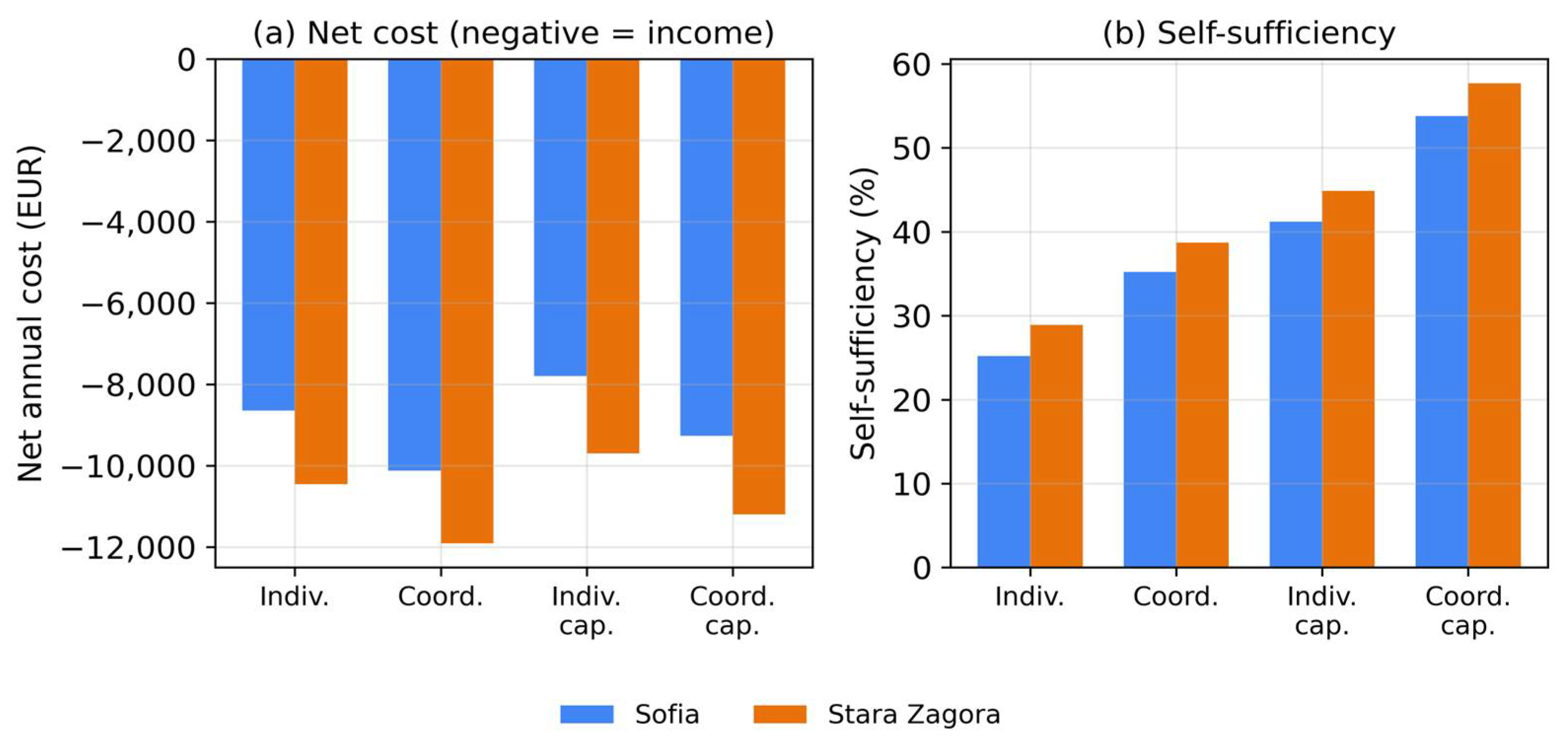
3.6. Scenarios and Indicators

Six configurations are compared per location: grid-only (loads supplied entirely from the grid, no PV revenue), PV-only (PV with negative-price curtailment but no storage), and PV with storage under the four dispatch variants. The evaluation indicators are the net annual energy cost (imports minus export revenue; negative values denote net income), reported separately from capacity charges, which are proportional to the peak; the PV self-consumption ratio SC, defined as the share of PV generation used within the community (one minus exported over generated energy); the self-sufficiency ratio SS, defined as the share of the consuming sites’ demand covered without grid import; the coincident peak community grid import; curtailed PV energy; and the equivalent full battery cycles, computed as total discharged energy divided by battery capacity. Because grid charging is permitted in the base case, SC is interpreted as a net-export-based accounting indicator rather than a strict physical tracing of PV-origin energy. Because the community includes a merchant plant whose business is to export, a low community self-consumption ratio is a structural feature rather than an inefficiency, and we interpret SC accordingly.

4. Results

4.1. Net Annual Cost

Table 2. Net annual community energy cost and coincident peak grid import (Sofia, trailing twelve months of IBEX day-ahead prices). Negative costs denote net income. Capacity-aware rows exclude the capacity payment itself; the ex-post capacity charges of the schedules under daily and monthly billing are reported in Section 4.5.

Configuration	Net Cost (EUR/yr)	Peak (kW)	Note
Grid only (loads, no PV)	+39,096	—	baseline
PV only (with curtailment)	+13,135	45	−66% vs. baseline
PV + BESS, independent (cost-only)	−8642	241	net income
PV + BESS, coordinated (cost-only)	−10,122	241	+1480 EUR vs. indep.
PV + BESS, independent (capacity-aware)	−7795	133	peak −45%
PV + BESS, coordinated (capacity-aware)	−9261	140	peak −42%

and Figure 2 report the net annual energy cost of the community in Sofia. The grid-only baseline—the two industrial loads supplied entirely from the grid—costs 39,096 EUR per year. Adding the three PV systems with contract-compliant curtailment reduces the net cost to 13,135 EUR (−66%). Storage changes the sign of the balance: under independent cost-only dispatch, the community earns a net 8642 EUR per year, and coordination raises the net income to 10,122 EUR—a further gain of 1480 EUR. Coordination is directly profitable under the real contract because every megawatt-hour shared internally avoids the full import price (day-ahead plus 30 EUR/MWh) while foregoing only the contract export price (day-ahead minus 2.15 EUR/MWh), a spread of roughly 32 EUR/MWh on all shared energy. The gain scales with this spread: at import adders of 15, 30 and 45 EUR/MWh the annual coordination gain is 1107, 1480 and 2032 EUR respectively, remaining strictly positive across the tested range.

4.2. Self-Consumption and Self-Sufficiency

Figure 3 shows the effect of coordination and of the objective on energy autonomy. PV self-consumption rises from 32.0% under independent operation to 41.0% under coordination, and the self-sufficiency of the two consuming sites increases from 25.2% to 35.2%. The absolute levels are structurally low because the community includes the merchant plant, whose 128 MWh of annual generation is produced to be sold; coordination redirects part of that output to cover P1 and P2 deficits whenever doing so beats the contract spread. Under the capacity-aware objective, both indicators rise further, to 56.4% and 53.8% respectively, because limiting the import peak implicitly favors serving load from local resources and storage rather than from concentrated cheap-hour imports.

4.3. Annual Energy Balances of the Community Members

Table 3. Annual energy balances of the community members under cost-only dispatch (Sofia, trailing twelve months; MWh/yr; values independently rounded, so sums may differ by ±0.1). The upper block refers to independent dispatch. The lower block refers to coordinated dispatch, in which the sites form a single settlement perimeter (Equation (8)): per-member grid flows are replaced by each member’s net internal position (injection positive), and external grid flows are defined at community level. Battery losses are charged minus discharged energy. PV self-consumption follows the net-export accounting of Section 3.6; it is not meaningful for P3, whose exports exceed its own generation owing to grid-charged arbitrage. Under coordination, per-member self-consumption is not uniquely defined without a tracing or allocation rule and is therefore reported only at community level.

Quantity	P1	P2	P3	Community
■ Independent dispatch
Available PV energy	104.0	62.4	128.1	294.5
Dispatched PV energy	101.9	61.8	124.6	288.4
Curtailed PV energy	2.1	0.6	3.5	6.1
Battery charge	54.6	50.7	112.8	218.1
Battery discharge	51.9	48.2	100.5	200.6
Battery losses	2.7	2.5	12.3	17.5
Grid import	90.9	75.9	42.7	209.4
Grid export	30.1	15.2	155.0	200.3
On-site consumption	160.0	120.0	0.0	280.0
PV self-consumption (%)	71.1	75.6	—	32.0
■ Coordinated dispatch (single settlement perimeter, Equation (8))
Dispatched PV energy	102.0	60.9	126.7	289.7
Curtailed PV energy	2.0	1.5	1.4	4.8
Battery charge	57.3	48.6	110.5	216.4
Battery discharge	54.5	46.2	98.4	199.1
Battery losses	2.8	2.4	12.0	17.3
Net site position at the community boundary (positive values denote surplus)	−60.8	−61.4	+114.7	−7.6
Community grid import	—	—	—	181.4
Community grid export	—	—	—	173.9
PV self-consumption (%)	—	—	—	41.0

complements the economic indicators with the annual energy balances of the three members and of the community as a whole under cost-only dispatch (Sofia). Under independent operation, P1 dispatches 101.9 MWh of its 104.0 MWh available PV resource (2.1 MWh curtailed), cycles 54.6/51.9 MWh through its battery, imports 90.9 MWh and exports 30.1 MWh against an on-site consumption of 160 MWh; P2 exhibits the same pattern at a smaller scale. The load-free merchant plant P3 dispatches 124.6 MWh of PV, imports 42.7 MWh—almost entirely low- and negative-price battery charging—and exports 155.0 MWh, more than its own PV production, the difference being grid-charged arbitrage energy. Battery losses absorb the difference between charged and discharged energy (17.5 MWh community-wide, consistent with the rated efficiencies). Coordination leaves the site-internal quantities nearly unchanged (P1, for instance, dispatches 102.0 MWh of PV and cycles 57.3/54.5 MWh through its battery), but the members’ roles become visible in their net positions at the community boundary: P1 and P2 draw 60.8 and 61.4 MWh net from the community perimeter, while the merchant plant injects 114.7 MWh net into it, covering the bulk of the industrial deficits internally. At community level, re-optimization and internal netting jointly reduce external imports from 209.4 to 181.4 MWh and external exports from 200.3 to 173.9 MWh. These annual changes in the external flows are not identical to the gross internally shared volume, because PV and battery dispatch are themselves re-optimized under coordination; the interval-by-interval gross shared volume—the quantity on which the coordination gain of Section 4.1 is earned and which the wheeling fee of Section 4.9 prices—is approximately 46 MWh per year. In the net-export accounting of Section 3.6, the per-member PV self-consumption is 71.1% for P1 and 75.6% for P2; for P3, the indicator is not meaningful, since the plant exports more energy than it generates.

4.4. Per-Site Analysis and the Value of the Battery Retrofit

Table 4. Per-site net annual cost under independent cost-only dispatch (Sofia). Negative values denote net income. The battery more than doubles the real merchant plant’s revenue under the offtake contract.

Prosumer Site	PV-Only (EUR/yr)	PV + BESS (EUR/yr)	Effect of Storage
P1 (manufacturing)	+11,188	+5892	−47% net cost
P2 (cold storage)	+11,335	+6296	−44% net cost
P3 (merchant plant)	−9388	−20,829	+122% net revenue

decomposes the independent cost-only scenario by site. For the producing consumers, storage roughly halves the net cost relative to PV-only operation (P1: 11,188 → 5892 EUR; P2: 11,335 → 6296 EUR). The most striking result concerns the real merchant plant: PV-only operation under the contract earns 9388 EUR per year, while the 261 kWh AC-coupled retrofit raises the net revenue to 20,829 EUR—an increase of 122%. The battery monetizes intraday price spreads by shifting the plant’s midday output into evening price peaks and by charging from the grid during negative-price hours, in which the plant would otherwise have to curtail; it also absorbs energy that the contract would penalize if injected. This single-site result is operationally promising for the many existing small PV plants operating under indexed offtake contracts, subject to the investment considerations discussed in Section 5.

4.5. Grid Interaction, Curtailment and Peak Demand

Figure 4 shows the community grid exchange over a representative summer week against the day-ahead price. Under the cost-only objective, batteries charge during low- and negative-price hours and during the midday PV surplus, discharge into the evening price peak, and the merchant plant’s exports track the price profile. Because all batteries respond to the same price signal, charging synchronizes in the cheapest hours: the coincident community import peaks at 241 kW, more than five times the 45 kW peak of the PV-only configuration, in both the independent and coordinated regimes—the aggregate battery power (205 kW) plus concurrent load.

Endogenous curtailment behaves as the contract intends: 6.1 MWh of available PV energy is curtailed per year under independent dispatch, falling to 4.8 MWh under coordination and to 1.8 MWh under the capacity-aware coordinated objective, as storage and internal sharing progressively absorb energy that would otherwise be injected at value-destroying prices.

The capacity-aware objective removes the peak side effect. As Figure 5 summarizes, pricing the daily peak cuts the coincident import to 133 kW (independent) and 140 kW (coordinated)—a 42–45% reduction—while the net income falls by only 847–861 EUR per year. Priced ex post at the assumed rate, the coordinated cost-only schedule incurs an annual capacity charge of 20.2 kEUR under daily billing (c_cap·Σ_d p_d over the 365 daily peaks; mean daily peak 158 kW) and 32.3 kEUR under equivalent monthly billing (10.6 EUR/kW per month applied to each month’s maximum import); the capacity-aware schedule reduces these to 3.7 and 8.2 kEUR, respectively (mean daily peak 29 kW). The avoided capacity cost of 16.5–24.1 kEUR per year therefore exceeds the foregone income by more than an order of magnitude under either billing convention, so the capacity-aware schedule is preferable whenever demand charges or binding connection limits apply. Net of these modeled charges, the capacity-aware coordinated schedule remains a net earner of 5.6 kEUR/yr under daily billing and 1.0 kEUR/yr under monthly billing, whereas the cost-only schedule incurs net costs of 10.1 and 22.2 kEUR/yr, respectively. The break-even capacity rate above which the capacity-aware schedule dominates is approximately 0.018 EUR/kW per day (equivalently, 0.38 EUR/kW per month)—about one twentieth of the assumed rate—so this conclusion does not hinge on the assumed magnitude.

4.6. Seasonal Pattern

Figure 6 shows the monthly community energy balance under coordinated cost-only dispatch. The available PV resource peaks in summer at roughly twice the winter level, while the industrial load is nearly flat. Exports consequently concentrate between April and September, when the merchant plant and the midday surpluses of P1 and P2 exceed community demand, whereas imports dominate from November to February. Storage smooths the intraday pattern but cannot bridge the seasonal gap—a well-known structural limit of daily cycle batteries that the figure makes explicit for this community.

4.7. Location Sensitivity: Sofia Versus Stara Zagora

Table 5. Location comparison for the trailing twelve months. The solar resource shifts the economics; the peak behavior is resource-invariant. Cost and income values exclude capacity charges (Section 4.5).

Indicator	Sofia	Stara Zagora	Difference
Specific PV yield (kWh/kWp)	1300	1390	+6.9%
Net cost, PV only (EUR/yr)	+13,135	+11,432	−13.0%
Net income, coordinated (EUR/yr)	10,122	11,905	+17.6%
Net income, coordinated cap.-aware (EUR/yr)	9261	11,194	+20.9%
Self-sufficiency, coord. cap.-aware (%)	53.8	57.7	+3.9 pp
Peak, cost-only/cap.-aware (kW)	241/140	241/140	—

and Figure 7 compare the two locations. The 6.9% higher specific yield of Stara Zagora (1390 versus 1300 kWh/kWp) translates into consistently better economics: net income under coordinated cost-only dispatch rises from 10,122 to 11,905 EUR per year (+17.6%), and self-sufficiency of the consuming sites improves by 3–4 percentage points across all variants. The peak-related conclusions are location-invariant—cost-only peaks of 241 kW and capacity-aware peaks of 132–140 kW in both cities—because the peak is driven by the aggregate battery power responding to the shared price signal, not by the solar resource. Since the real P3 plant is located in the EVN distribution area of southern Bulgaria, the Stara Zagora scenario is the more representative one for the retrofit case, and it strengthens the corresponding result: the battery raises the plant’s annual revenue by a factor of 2.1–2.2 in either resource (

Table 6. Net annual revenue of the real 98.56 kWp merchant plant (P3) with and without the 261 kWh AC-coupled battery retrofit, by location and charging arrangement. Negative values denote net income; the PV-only-charging column is the conservative variant in which grid-charged re-export is disallowed (Section 4.9).

Location (P3 Retrofit)	PV-Only (EUR/yr)	PV + BESS, Grid Charging (EUR/yr)	PV + BESS, PV-Only Charging (EUR/yr)	Uplift
Sofia	−9388	−20,829	−19,719	+110–122%
Stara Zagora	−10,054	−21,545	−20,510	+104–114%

).

4.8. Battery Utilization

Under cost-only dispatch, the batteries perform 462, 429 and 385 equivalent full cycles per year for P1, P2 and P3, respectively, when operated independently, and 484, 411 and 377 cycles when coordinated—slightly more than one cycle per day, consistent with combined solar-shifting and price arbitrage (coordination shifts additional cycling onto the largest hybrid unit). Relative to cost-only coordination, the capacity-aware coordinated schedules are gentler across all three units (361, 349 and 297 cycles), since the community import cap curtails aggressive arbitrage bursts—including the grid-charged arbitrage of the load-free merchant plant. Against the 8000-cycle rating of the LiFePO4 systems, all schedules imply a calendar-limited rather than cycle-limited lifetime, confirming that the reported economics do not rest on unrealistically aggressive cycling.

4.9. Robustness and Sensitivity Analyses

Seven further checks probe the assumptions most likely to be questioned. First, grid charging of the merchant plant’s battery: if P3 is restricted to charging exclusively from its own PV—the conservative reading of the offtake contract—its net annual revenue decreases from 20,829 to 19,719 EUR in Sofia (and from 21,545 to 20,510 EUR in Stara Zagora). Grid-charged arbitrage thus contributes only about 5% of the retrofit revenue, and the headline result is robust to this contractual interpretation: the battery still more than doubles the plant’s income (×2.10; see Table 6).

Second, wheeling charges on internally shared energy: levying a fee of 10 (20) EUR/MWh on every megawatt-hour shared within the community reduces the annual coordination gain from 1480 to 1144 (882) EUR, while the optimally shared volume adapts downward from roughly 46 to 32 (21) MWh. Coordination therefore remains profitable under any wheeling charge below the import–export spread, with the community endogenously scaling back sharing as the fee rises.

Third, settlement resolution: re-solving January–May 2026—the period with native 15 min market data—at quarter-hourly resolution (LP relaxation, verified ex post to be tight for the cost-only objective; see the discussion of the binary constraints (5) in Section 3.4) increases the window net income from 2007 to 3098 EUR under independent operation and from 2487 to 3682 EUR under coordination. Hourly averaging therefore smooths intra-hour price extremes and understates the achievable arbitrage value by roughly 1.1–1.2 kEUR over the five-month window; the annual results reported above are accordingly conservative lower bounds, and the coordination gain is essentially unchanged across resolutions. The coincident peak import is likewise resolution-invariant (241 kW hourly versus 246 kW at 15 min resolution, a 2% difference), since it is set by the aggregate battery power rather than by price granularity.

Fourth, the terminal-state treatment: replacing the terminal valuation of stored energy in (1) with a hard restoration of every battery to 50% state of charge at the end of each day changes the annual result from −8642 to −8312 EUR under independent operation and from −10,122 to −9797 EUR under coordination (−3.8% and −3.2% of net income), while the coordination gain is essentially unchanged (1480 versus 1485 EUR). The end-of-horizon handling therefore does not drive the reported effects.

Fifth, forecast errors: to bound the value of the perfect-foresight assumption, we run a Monte Carlo experiment with 30 realizations per error level (realization i uses random seed 500 + i for σ = 5% and 1000 + i for σ = 10%), in which multiplicative Gaussian day-ahead errors, independent across hours and clipped to ±50%, are imposed on both PV availability and load. Each site commits to the schedule optimized on the forecast; in the realization, the battery follows the committed schedule—so the state-of-charge trajectory remains feasible by construction—dispatched PV is capped by the actual resource, the grid absorbs all deviations, and injection is stopped whenever the contract price is negative. Deviations are valued using the same day-ahead import/export price functions as in the base model; balancing-market prices and imbalance penalties remain excluded. The realized independent-regime income is 8034 ± 8 EUR (mean ± standard deviation; 5–95th percentile range 8024–8048 EUR) at σ = 5% and 7427 ± 19 EUR (7402–7456 EUR) at σ = 10%, versus 8642 EUR under perfect foresight (−7% and −14%). The dispersion across realizations is small because annual aggregation averages out hourly errors; the systematic loss is the cost of committing to schedules built on imperfect forecasts. Day-ahead prices themselves are known at scheduling time, so no price-forecast error is involved. The framework thus remains strongly net-positive on an energy-only basis at the tested 5–10% forecast-error levels, and replacing perfect foresight with forecast-driven and rolling-horizon control remains part of the research program of Section 5.

Sixth, degradation-aware dispatch: we add an explicit throughput cost c_deg per MWh of discharged energy to the objective and re-solve the P3 retrofit case. With a turnkey cost of 300–500 EUR/kWh and the 8000-cycle rating, the full-cycling throughput cost is 42–69 EUR/MWh; since the observed cycling (under 400 equivalent full cycles per year) implies a calendar- rather than cycle-limited life, c_deg = 20–40 EUR/MWh spans the plausible range of the marginal cycling cost. The optimizer responds by cycling less aggressively (324 and 281 instead of 385 equivalent full cycles per year) and the market revenue decreases from 20,829 to 20,409 and 19,561 EUR, respectively; net of the degradation provision itself, the retrofit still earns 18,717 and 16,621 EUR per year—an uplift of +99% and +77% over PV-only operation. The headline conclusion that storage substantially raises the merchant plant’s revenue is therefore robust to degradation costing.

Seventh, alternative industrial load profiles: replacing the base shapes with a two-shift manufacturing plateau at P1 and a nearly flat continuous process at P2 (same annual energies) reduces the absolute income by approximately 17–20% (independent: 8642 → 6956 EUR; coordinated: 10,122 → 8386 EUR), reflecting the weaker price alignment of the alternative shapes, while preserving the sign of the result and changing the coordination premium by less than 4% (1480 → 1430 EUR). The qualitative conclusions—storage turns the community into a net earner on an energy-only basis and coordination adds a further, spread-driven gain—are thus insensitive to the exact profile shape, although the absolute income level does depend on it.

5. Discussion

The results quantify a clear hierarchy of value for an industrial prosumer community under real market conditions. PV with contract-compliant curtailment captures the first tranche, cutting the community’s net cost by two thirds. Storage captures the second and largest tranche, turning the community into a net earner on an energy-only basis by shifting energy from low- and negative-price hours into evening peaks. Coordination adds a third tranche whose magnitude is set by the contract spread: with imports at the day-ahead price plus 30 EUR/MWh and exports at the day-ahead price minus 2.15 EUR/MWh, every internally shared megawatt-hour is worth roughly 32 EUR, which the community realizes on the energy redirected from the merchant plant and the midday surpluses to the industrial loads.

The contractual anchoring changes qualitative conclusions, not just numbers. Under the stylized 90–of-spot export remuneration common in the literature, our earlier experiments found coordination’s monetary benefit to be negligible for export-oriented communities; under the contract, with its narrow export discount and negative-price pass-through, coordination is directly profitable within the modeled day-ahead settlement—with a gain that grows with the import price spread (Section 4.1)—and endogenous curtailment becomes an active lever that storage progressively displaces (from 6.1 to 1.8 MWh per year across variants). Models that ignore the actual remuneration structure can therefore misjudge both the value of cooperation and the role of curtailment.

The retrofit result is the most operationally promising finding. The 98.56 kWp merchant plant, of which there are thousands on indexed offtake contracts across the region, more than doubles its net revenue (+122% in Sofia, +114% in the southern resource) by adding a single commercially available 261 kWh AC-coupled cabinet, without touching the existing PV inverter.

The battery earns on three margins simultaneously: intraday arbitrage on the plant’s own output, grid-charged arbitrage during negative-price hours, and avoided negative-price penalties that would otherwise force curtailment. The reported uplift should accordingly be read as the value under a metering arrangement that permits grid charging and export settlement at the contract price; the conservative PV-only-charging variant (Section 4.9 and Table 6) trims it by only about 5%. These figures are gross operational gains: capital expenditure, degradation beyond cycle counting, balancing costs, taxes and financing are not modeled. The degradation-priced dispatch of Section 4.9 bounds the first of these effects: even with a conservative provision of 40 EUR/MWh of discharged energy, the retrofit retains about three quarters of its gross uplift. As an illustrative order of magnitude only,

Table 7. Illustrative simple-payback sensitivity for the P3 battery retrofit (Sofia, grid-charging variant; gross annual uplift of 11.4 kEUR/yr from Table 6). Illustrative only—not a bankable investment appraisal: degradation beyond cycle counting, balancing costs, taxes and financing are excluded.

Battery CAPEX (EUR/kWh)	System Cost (kEUR, 261.24 kWh)	Gross Annual Uplift (kEUR/yr)	Simple Payback (yr)
300 (low)	78.4	11.4	6.9
400 (medium)	104.5	11.4	9.1
500 (high)	130.6	11.4	11.4

reports the simple payback of the P3 retrofit across a plausible turnkey-cost range for commercial LiFePO4 systems; this is illustrative only, not a bankable investment appraisal, and a rigorous, financed assessment remains future work.

The peak trade-off carries the main system-level lesson. Because cost-only dispatch is blind to power, all batteries charge simultaneously in the cheapest hours and the coincident import peak rises more than fivefold relative to PV-only operation—an outcome that would be expensive under capacity charges and unwelcome for the distribution network. Internalizing the peak reverses the picture at almost no cost: the capacity-aware community keeps over 90% of its income while cutting the peak by 42%, effectively converting itself from a peak amplifier into a provider of peak-shaving flexibility. The asymmetry of the exchange—hundreds of euros of foregone income against 16.5–24.1 kEUR of avoided capacity charges under daily and monthly billing (Section 4.5)—suggests that capacity-aware objectives should be the default for community energy management systems rather than an optional refinement.

Several limitations should be noted. The load profiles of P1 and P2 are representative rather than metered, and the PV resource is modeled rather than measured; both can be replaced by site data without changing the method, and the P3 plant’s metered production will serve exactly this purpose in future work. The base optimization assumes perfect PV and load foresight within each day, while day-ahead prices are treated as known at scheduling time; intraday and balancing dynamics, including the balancing costs that the contract allocates to the producer, are not modeled; the realized-cost impact of imperfect day-ahead forecasts is bounded in Section 4.9. Hourly averaging of the market’s 15 min settlement periods smooths some price extremes and therefore understates arbitrage value; Section 4.9 quantifies this effect and shows that the reported annual economics are conservative lower bounds. Battery degradation is priced implicitly through the cycle count and explicitly through the degradation-priced sensitivity of Section 4.9, the capacity rate is an illustrative scenario assumption, the daily peak term approximates monthly demand charges, and the model represents each site at a single AC node without network physics. The coordinated regime additionally presupposes frictionless community netting; the Bulgarian shared-energy framework in force since February 2026 and the frictions and charges it introduces are discussed in Section 3.4. Within the tested sensitivity ranges, these limitations do not reverse the principal operational findings, although broader parameter ranges or different settlement rules could change both their magnitude and, in some cases, their sign.

These limitations define a coherent research program: ingesting metered load, production and settlement data from the real sites; replacing perfect foresight with forecast-driven and reinforcement-learning controllers benchmarked against the MILP bound; adding balancing-cost and degradation-aware terms; extending the peak formulation to rolling monthly demand charges; and scaling from three sites to larger communities with multi-agent coordination. The simulation environment presented here—measured market prices, contractual terms, commercial hardware envelopes, and a transparent optimization core—is designed to serve as the data-generating foundation for that program.

6. Conclusions

We presented a reproducible, contract-anchored simulation environment for an industrial prosumer community comprising two producing consumers with DC-coupled hybrid storage and a real 98.56 kWp merchant PV plant retrofitted with a 261 kWh AC-coupled battery, dispatched with a daily MILP against one full year of real IBEX day-ahead prices under the terms of a real market offtake contract. Under these conditions, PV with contract-compliant curtailment cut the community’s net annual cost from 39.1 to 13.1 kEUR; on an energy-only basis, before capacity charges, storage turned the community into a net earner (8.64 kEUR/yr independently, 10.12 kEUR/yr coordinated); and the battery retrofit more than doubled the merchant plant’s revenue (+122%; gross of degradation and capital costs, which the degradation-priced sensitivity of Section 4.9 and the payback bounds of Table 7 quantify). Cost-only dispatch inflated the coincident grid peak from 45 to 241 kW, whereas a capacity-aware objective restored it to 133–140 kW while preserving over 90% of the income—an exchange favorable under the tested capacity-charge conventions, under which only the capacity-aware schedule remains net-positive after the modeled charge. The sunnier Stara Zagora resource increased the coordinated-storage income by approximately 17–21% and improved the PV-only net cost by 13%, while leaving the peak behavior unchanged. The environment provides a realistic basis for studying individual and collective prosumer behavior and for developing forecasting and control methods on top of real market and contractual data.