Systematic Evaluation of Top-K Neighborhood in Emotion-Aware Literature Book Recommendation

Abstract

Literature books recommender systems often overlook the vital affective dimensions that dictate reading preferences. To address this, we present an emotion-aware recommendation framework that leverages latent emotional profiles extracted from user reviews. By constructing an emotional embedding space, the system maps the affective resonance of books and aligns them with historical user preferences. This study specifically investigates the sensitivity of neighborhood size, defined as the number of nearest neighbors ($Top-K$), and emotional similarity evaluation thresholds ($\tau$) within affective-based collaborative filtering. Through a systematic empirical evaluation across four nested datasets, we demonstrate that affective recommendation alignment is highly dependent on neighborhood size. Our findings identify $Top-K=3$ as an effective neighborhood parameter, successfully balancing highly affective aligned item acquisition while neutralizing the data noise introduced by larger user clusters. Robustness analysis shows that the proposed framework maintains high affective recommendation alignment under strict similarity constraints.

1. Introduction

Recommender systems in the domain of literature primarily rely on collaborative filtering, which identifies user preferences based on shared interaction histories. However, these methods frequently fail to account for the latent affective dimensions of reading, the emotional state or mood that drives user preference [1]. While item-based features such as genre and author serve as a baseline for similarity, they do not fully capture the qualitative user experience. User reviews represent a critical but underutilized resource in this context, as they contain rich semantic information encompassing opinions, preferences, and emotional reactions [2,3]. Emotion-aware recommender systems seek to bridge this gap by explicitly incorporating users’ affective states and emotional preferences into the recommendation process [4].

Recent advances in affective computing have seen a transition toward transformer-based emotion recognition models and fine-grained sentiment analysis techniques that capture deep contextual nuances [5,6]. While these neural architectures offer high predictive power, they often function as black boxes, demand substantial computational resources, and can overfit to the kind of noisy or informal text that is commonplace in literary reviews. In contrast, lexicon-based emotion frameworks such as structured affective word lists provide high interpretability, computational efficiency and transparent mapping of emotional dimensions.

This paper presents a recommendation framework that integrates latent emotional profiles extracted from user reviews. By adopting a lexicon-driven methodology, we ensure emotional profiles that bridge the gap between interpretable affective analysis and neighborhood-based collaborative filtering. Furthermore, this approach constructs an emotional embedding space to characterize the affective resonance of literary works, aligning them with the user’s historical emotional preferences.

We investigate the affective alignment dynamics within neighborhood-based collaborative filtering. While several studies have examined the influence of neighborhood size on recommendation performance [7,8], the specific dynamics of affect-based filtering when using emotion-aware data remain underexplored [9,10]. This work addresses the above gap through a systematic evaluation of varying neighborhood sizes ($Top-K\in \{1,3,5,7,10\}$), guided by the following research questions:

• RQ1: How does recommendation affective alignment vary systematically with neighborhood size when user similarity is computed exclusively from affective embeddings derived from user reviews?
• RQ2: Does an effective neighborhood size ($Top-K$) exist?
• RQ3: How do emotional similarity thresholds ($\tau$) influence the affective alignment of recommendations generated across varying neighborhood sizes ($Top-K$)?

Our contributions are twofold: we first establish a robust mechanism for mapping literary works to emotional profiles, then provide an empirical analysis of how these profiles improve affective alignment of the recommendations across varying neighborhood sizes and similarity thresholds. The main contributions can be summarized as follows:

• Proposal of a model for representing books and modeling user preferences, which integrates emotions identified in social media reviews and the collaborative filtering recommendation method.
• Systematic evaluation of neighborhood size ($Top-K$) on recommendation affective alignment, demonstrating that affective recommendation alignment varies systematically when user similarity is calculated using emotional embeddings.
• Identification of $Top-K=3$ as an effective neighborhood parameter which balances personalized candidate acquisition against mitigation of noise introduced by larger neighborhoods with less affective alignment.
• A systematic analysis of model robustness through a comparative analysis across four nested datasets and similarity thresholds ($\tau$), confirming that the system maintains high affective recommendation alignment even under stringent threshold constraints.
• A performance comparison against prior approaches [11,12], demonstrating measurable improvements in terms of affective recommendation alignment.

2. Related Work

Modern collaborative filtering frameworks frequently integrate auxiliary data sources such as text, features, or scenarios in order to mitigate sparsity and improve baseline representations. For instance, Karabila et al. [13] designed a model fusing collaborative filtering with a sequential Bi-LSTM network to extract user sentiment from textual reviews, substantially raising personalization accuracy. Similarly, the Emotion-Aware Recommender System (EARS) [4] constructs multi-channel user profiles by optimizing a matrix factorization pipeline using explicit ratings, implicit social networks, and review-driven emotional indicators. Sun and Liu [14] mapped interaction matrices into low-dimensional latent spaces using a hybrid K-Nearest Neighbors (KNN) and non-negative matrix factorization algorithm called KNNCNMF, speeding up execution via efficient dot product similarity. Additionally, handling complex cross-domain environments, Liu et al. [15] introduced MultiFS, an automated multi-scenario feature selection framework that uses hierarchical gate vectors to isolate domain-exclusive features and resolve data distribution imbalances.

Beyond broad feature fusion, the recent literature has shifted from flat similarity pairs towards advanced topological and hierarchical neighborhood definitions. Within graph neural networks, Yan et al. [16] introduced SNE–GCN, which leverages an attention-based mechanism to explicitly aggregate second-order neighbors with first-order edges. This approach enriches node representations while preventing over-smoothing. Alternatively, hierarchical trees and adaptive profiles have been used to capture complex proximity paths; for example, Koohi and Kiani [17] developed a parameter-free neighbor-finding method via subspace clustering that organizes users into a three-level tree based on item interest categories, enabling a specialized metric to discover hidden but indirectly similar users. User context can also be used to dynamically adjust neighbor profiles; Subramaniyaswamy and Logesh [18] proposed an Adaptive KNN (AKNN) model backed by a domain ontology, which splits users into the distinct categories of minion (new users) and prominent (old users) in order to eliminate cold-start limitations.

Crucially, the ultimate performance of these systems remains tightly bound to hyperparameter calibration, particularly regarding the selection and scalability of neighborhood sizes. Examining these baseline limits, Airen and Agrawal [19] evaluated multiple KNN variants on the MovieLens-100K dataset, demonstrating that predictive accuracy stabilizes once the user neighborhood reaches a fixed threshold of $K=40$ neighbors, although the model faces severe runtime bottlenecks at scale. The risk of rigid neighborhood boundaries is also highly evident in cross-domain settings; Kim and Cho [20] applied a KNN collaborative pipeline to restore missing subsurface log data, noting that the optimal neighborhood size K varies drastically per data instance and that standard error calculations fail to isolate a reliable value. Finally, Dokoupil and Peska [8] investigated the structural impacts of fluctuating cluster sizes on collaborative algorithms, demonstrating that different similarity metrics yield entirely separate neighborhood statistics as scales expand. Collectively, these studies establish that the size of a user neighborhood acts as a vital structural determinant of performance rather than a passive hyperparameter, motivating our investigation.

3. System Design

We propose a system for obtaining book recommendations using a collaborative filtering technique and limited neighborhood sizes.

In what follows, we introduce the data model of our proposed system. The book space $\mathcal{B}$ refers to the set of books and the review space $\mathcal{R}$ to the set of reviews, while the review space ${\mathcal{R}}_B$ refers to the set of reviews for book B, $B\in \mathcal{B}$. The user space $\mathcal{U}$ refers to the set of users, while the book space ${\mathcal{B}}_U$ refers to the set of books reviewed by user U, $U\in \mathcal{U}$. Finally, the emotion space $\mathcal{E}$ refers to the set of 35 predefined emotions from [21], as defined in Equation (1).

$$\begin{array}{cc}\mathcal{E}=& \{\mathit{adequate}, \mathit{alone}, \mathit{angry}, \mathit{anxious}, \mathit{apathetic}, \mathit{attached}, \mathit{attracted}, \mathit{average},\\ & \mathit{belittled}, \mathit{bored}, \mathit{burdened}, \mathit{cheated}, \mathit{codependent}, \mathit{demoralized}, \mathit{derailed},\\ & \mathit{ecstatic}, \mathit{embarrassed}, \mathit{entitled}, \mathit{esteemed}, \mathit{fearful}, \mathit{fearless}, \mathit{focused}, \mathit{free},\\ & \mathit{happy}, \mathit{hated}, \mathit{independent}, \mathit{lost}, \mathit{loved}, \mathit{lustful}, \mathit{obsessed}, \mathit{powerless}, \mathit{sad},\\ & \mathit{safe}, \mathit{singled}\mathit{out}, \mathit{surprise}\}\end{array}$$

(1)

A book B is defined as a tuple (Equation (2)):

$$B=(I{D}_B,E{M}_B),B\in \mathcal{B}$$

(2)

where $I{D}_B$ represents the unique identifier of the book and $E{M}_B$ refers to the Book Emotional Representation (Equation (3)), a 35-dimensional vector in which each element $e{m}_i$ represents the density of emotion $e_i\in \mathcal{E}$ across the set of reviews.

$$E{M}_B=[e{m}_1,e{m}_2,\dots ,e{m}_{35}]$$

(3)

The input space $\mathcal{I}$ refers to the set of inputs for the system. An input $\in \mathcal{I}$ is defined as a triple (Equation (4)):

$$input=(B,U,EM-rev)$$

(4)

where $B\in \mathcal{B},U\in \mathcal{U}$, and $EM-rev$ is a 35-dimensional vector (Equation (5)):

$$EM-rev=[f{r}_1,f{r}_2,\dots ,f{r}_{35}]$$

(5)

with $f{r}_i$ representing the density of emotion $e_i\in \mathcal{E}$ within the review text.

The reviews corresponding to user U are defined as a set (Equation (6)):

$${\mathcal{I}}_U=\{(B,U,EM-rev)\in \mathcal{I}\}.$$

(6)

A user U is defined as a tuple (Equation (7)):

$$U=(I{D}_U,E{M}_U),U\in \mathcal{U}$$

(7)

where $I{D}_U$ represents the unique user ID and $E{M}_U$ represents the emotional profile of user U (Equation (8)):

$$E{M}_U=\sum _{(B,U,EM-rev)\in {\mathcal{I}}_U}EM-rev.$$

(8)

Next, we detail the computational pipeline stages. The first step is to apply data cleaning to the reviews, which includes lowercasing, punctuation normalization, tokenization, and stopword removal. Next, the emotional features are extracted. For this, the cleaned text is processed by using an external lexicon-based mapping method to classify the affective content. The lexicon is defined in [21], and has been incorporated and evaluated in prior emotion analysis and psycholinguistic research as a standard source for establishing affective word lists [22,23]. The lexicon contains a set of words and the associated emotions. As a result, each book review is represented as a vector (Equation (9)):

$$EM-rev=[f{r}_1,f{r}_2,\dots ,f{r}_{35}]$$

(9)

where $f{r}_i$ is the frequency of linguistic markers for emotion $e_i\in \mathcal{E}$ identified within the review.

Each component $e{m}_i$ of the Book Emotional Representation is a normalized value representing the relative frequency of the emotions extracted from the book B review corpus ${\mathcal{R}}_B$ (Equation (10)):

$$e{m}_i={\displaystyle \frac{f_i}{{\sum }_{k=1}^{35}{f}_k}},e{m}_i\in [0,1].$$

(10)

The recommendation strategy focuses on retrieving books that align with the preferences of emotionally similar users.

Two users, A and B, share a degree of similarity based on their commonly reviewed books and the similarity of the reviews identified within the shared reviews. This similarity is computed using the cosine similarity (Equation (11)):

$$sim(A,B)={\displaystyle \frac{E{M}_A^{\left(AB\right)}·E{M}_B^{\left(AB\right)}}{\left|\right|E{M}_A^{\left(AB\right)}\left|\right|·\left|\right|E{M}_B^{\left(AB\right)}\left|\right|}}$$

(11)

where $E{M}_A^{\left(AB\right)}$ (Equation (12)) and $E{M}_B^{\left(AB\right)}$ (Equation (13)) are the user emotion vectors on shared books:

$$E{M}_A^{\left(AB\right)}=\sum _{\begin{array}{c}(B,U,EM-rev)\in {\mathcal{I}}_A\\ B\in {\mathcal{B}}_{A\cap B}\end{array}}EM-rev,$$

(12)

$$E{M}_B^{\left(AB\right)}=\sum _{\begin{array}{c}(B,U,EM-rev)\in {\mathcal{I}}_B\\ B\in {\mathcal{B}}_{A\cap B}\end{array}}EM-rev.$$

(13)

For new users, similarity is computed exclusively based on the book currently being reviewed, which is commonly reviewed by the target user and the $top-K$ similar users. In contrast, for registered users, similarity calculation also incorporates previously reviewed books from historical data.

The collaborative filtering recommendation algorithm is presented in Algorithm 1. The algorithm receives as input a user review $(B,U,EM-rev)$.

First, the scores for all users are computed depending on their shared emotions with user U for the commonly reviewed books. Next, the $Top-K$ most similar users are determined. To select the $Top-K$ neighbors, candidate users are ranked in descending order based on their similarity scores. In case of identical scores, the candidates are randomly selected with probabilities proportional to the number of reviews available for each candidate in the dataset.

The book preferences of the $Top-K$ similar users are determined and stored within an array called $books$. The preferences of the $Top-K$ similar users refer to the books that the users have positively reviewed and rated with 4 or 5 stars. In cases where the reviewed book has no prior reviewers, no overlapping user history can be established to find similar users, resulting in an empty list of recommendation candidates ($len\left(books\right)=0$).

We identify three major use cases of performing recommendations, depending on the number of requested recommendations $nREC$ and the number of recommendation candidates identified $len\left(books\right)$:

(i)

$len\left(books\right)=nREC$: The number of recommendation candidates is equal to the number of requested recommendations, which means that the entire list of candidates will be recommended to the user.

(ii)

$len\left(books\right)>nREC$: The number of recommendation candidates is greater than the number of requested recommendations, which means that the system will select $nREC$ candidates from $books$ and provide them as recommendations. The $nREC$ candidates are randomly selected with probabilities proportional to both the similarity of the neighborhood user and the specific rating assigned within the review.

(iii)

$len\left(books\right)<nREC$: The number of recommendation candidates is smaller than the number of requested recommendations, meaning that the $books$ list does not contain enough candidates to satisfy the number of recommendations requested $nREC$. We identify two sub-cases:

a.

$len\left(books\right)=0$: The recommendation list will be filled with $nREC$ completely random books from the dataset.

b.

$len\left(books\right)>0$: The recommendation list will contain the $books$ identified as candidates based on similar users’ preferences, and will be completed with $nREC-len\left(books\right)$ random books from the dataset.

Algorithm 1 Neighbor-Based Collaborative Filtering Recommendation Algorithm

Require: $top-K,nREC,\mathcal{B},\mathcal{U}$   1: Get user input review $(B,U,EM-rev)$   2: for each $user\in \mathcal{U}\setminus U$ do   3:       $score\left[user\right]\leftarrow sim(E{M}_{user},E{M}_U)$   4: end for   5: Create list of $top-K$ most similar users of U based on $score$   6: Identify $books$ enjoyed by similar users   7: if  $len\left(books\right)==nREC$  then   8:       Recommend $books$   9: else 10:       if $len\left(books\right)>nREC$ then 11:             Recommend $nREC$ random books from $books$ 12:       else 13:             while $len\left(books\right)<nREC$ do 14:                  Add in $books$ random book from the books dataset $\mathcal{B}\setminus books$ 15:             end while 16:             Recommend $books$ 17:       end if 18: end if

4. Experimental Results and Discussion

4.1. Dataset Overview

The experimental datasets were collected from the Goodreads website for purely academic purposes using our customized web scraper.

The experimental datasets correspond to the top 100, 500, 1000, and 2000 books tagged by users as “Best Books Ever” in the Goodreads website. Considering that each dataset contains a top list of the specific books category, it follows:

$$Dataset1\subset Dataset2\subset Dataset3\subset Dataset4$$

For experiments, the Goodreads datasets were split into 80% training and 20% testing using stochastic sampling and preservation of the per-book review distribution. The algorithm for the splitting procedure is described in Algorithm 2. The training reviews are used to create the emotional profile of the books, while the testing reviews are used to simulate a population of users writing reviews and seeking book recommendations.

Algorithm 2 Training–Testing Dataset partitioning considering per-book review distribution

Require: Reviews Dataset $\mathcal{R}$, Books Dataset $\mathcal{B}$, Target Test Ratio $r=0.20$ Ensure: Training Partition ${\mathcal{R}}_{\mathrm{train}}$, Testing Partition ${\mathcal{R}}_{\mathrm{test}}$   1: ${\mathcal{R}}_{\mathrm{train}}\leftarrow \varnothing$, ${\mathcal{R}}_{\mathrm{test}}\leftarrow \varnothing$   2: for each book $b\in \mathcal{B}$ do   3:       ${\mathcal{R}}_b\leftarrow \{\mathrm{review}\in \mathcal{R}\mid \mathrm{review}.\mathrm{book}\_\mathrm{id}=b.id\}$   4:       $N_b\leftarrow \left|{\mathcal{R}}_b\right|$   5:       $k_b\leftarrow \lceil N_b\times r\rceil$   6:       ${\mathcal{I}}_{\mathrm{test}}\leftarrow \mathrm{RandomSampleIndices}([0,N_b],\mathrm{count}=k_b)$   7:       for $i=0$ to $N_b-1$ do   8:           if $i\in {\mathcal{I}}_{\mathrm{test}}$ then   9:              ${\mathcal{R}}_{\mathrm{test}}\leftarrow {\mathcal{R}}_{\mathrm{test}}\cup \left\{{\mathcal{R}}_b\left[i\right]\right\}$ 10:           else 11:              ${\mathcal{R}}_{\mathrm{train}}\leftarrow {\mathcal{R}}_{\mathrm{train}}\cup \left\{{\mathcal{R}}_b\left[i\right]\right\}$ 12:           end if 13:       end for 14: end for 15: return  ${\mathcal{R}}_{\mathrm{train}},{\mathcal{R}}_{\mathrm{test}}$

The statistics of the reviews datasets are presented in

Table 1. Review dataset statistics (average values per ten iterations ± standard deviation).

Dataset	Total	Training	Testing
Dataset 1	13,957	11,149 ± 4	2808 ± 4
Dataset 2	70,401	56,223 ± 7	14,178 ± 7
Dataset 3	129,713	103,593 ± 56	26,119 ± 56
Dataset 4	245,015	195,637.9 ± 55	49,377 ± 55

. We observe that as the size of the dataset increases, the deviation of the number of training–testing reviews increases. This is due to the fact that the books are ordered within the “Best Books Ever” category based on book popularity in terms of users interactions, which means that lower-ranking books have a smaller number of reviews.

We classify the experimental subjects into two distinct categories: registered users and new users. Registered users represent individuals who are considered to have previously interacted with the system by writing reviews from the training dataset, allowing the system to model their long-term preferences. Conversely, new users represent a cold-start scenario, having no prior interactions with the system.

Table 2. User type statistics (average values per ten iterations ± standard deviation).

Dataset	Reg. User	New User	Reg. User%	New User%
Dataset 1	2133 ± 17	675 ± 18	76 ± 0.6	24 ± 0.6
Dataset 2	11,119 ± 28	3060 ± 30	78 ± 0.1	22 ± 0.2
Dataset 3	20,700 ± 72	5419 ± 33	79 ± 0.2	21 ± 0.1
Dataset 4	38,943 ± 65	10,434 ± 42	$78\pm$0.1	21 ± 0.1

presents the average user type statistics across the experimental scenarios along with the standard deviations.

4.2. Experimental Setup

To evaluate the performance of the proposed system, we employ Monte Carlo cross-validation (ten iterations). In each iteration, the reviews corpus is partitioned into 80% training reviews and 20% testing reviews, preserving the per-book review distribution.

We define the following parameters for a rigorous definition of our evaluation system:

–

The training reviews space $TrR$ refers to the total number of input reviews which are used for defining the emotional book representation $E{M}_B$.

–

The testing reviews space $TstR$ refers to the total number of input reviews seeking recommendations.

–

A recommendation $f\left(input\right)$ is the output returned by the recommendation algorithm as a set of $nREC$ books $B\in \mathcal{B}$ (Equation (14)):

$$f:TstR\to {\mathcal{B}}^{nREC},f\left(input\right)=(r_1,r_2,\dots ,r_{nREC}).$$

(14)

We use the following performance measures to evaluate our system: Coverage, Randomness Degree Assessment, and Affective Alignment Rate. While traditional collaborative filtering evaluation relies on historical item ratings evaluated via ranking metrics, our framework focuses on evaluating affective alignment and retrieval of user emotions. A limitation of this approach is that it evaluates the consistency of alignment with the emotional profile rather than the validation of independent predictive preference.

–

The Coverage (catalog coverage) determines the proportion of books from $\mathcal{B}$ that the system is able to recommend at least once across one iteration using the recommendation algorithm (Equation (15)).

$$Coverage={\displaystyle \frac{{\bigcup }_{input\in TstR}f\left(input\right)}{\left|\mathcal{B}\right|}}$$

(15)

–

The Randomness Degree Assessment (RDA) determines the level of stochastic influence in the recommendation process by categorizing results into three distinct categories:

• General Recommendation (GRL) corresponds to the case in which the set of books enjoyed by similar users contains at least $nREC$ books; this is Algorithm 1 use case $len\left(books\right)\ge nREC$.
• Random Fill Recommendation (RF) corresponds to the case in which the set of books enjoyed by similar users contains books, but they are fewer in number than $nREC$, meaning that the list of recommendations needs to be completed using a set of random books from the dataset; this is Algorithm 1 use case $0<len\left(books\right)<nREC$.
• Fully Random Recommendation (FR) corresponds to the case in which the set of books enjoyed by similar users is empty, and the user is recommended a completely random set of $nREC$ books; this is Algorithm 1 use case $len\left(books\right)=0$.

–

The Affective Alignment Rate ($AAR$) shows the proportion of recommendations $f\left(input\right)$ identified as recommendations with affective alignment based on the user’s emotional history. A recommendation $r_x$, $x\in \{1,2,\dots ,nREC\}$ is considered to possess affective alignment if the emotional profile of the recommended book matches the emotional profile of the user above a certain similarity threshold $\tau$. The similarity is computed using the cosine similarity (Equation (16)). To improve readability, the Affective Alignment Rate is reported as a percentage (Equation (17)).

$$AAR={\displaystyle \frac{{\sum }_{(B,U,EM-rev)\in TstR}{\sum }_{x=1}^{nREC}\mathbb{I}(\frac{E{M}_U·E{M}_{rx}}{\left|\right|E{M}_U\left|\right|·\left|\right|EMrx\left|\right|}\ge \tau )}{\left|TstR\right|·nREC}}$$

(16)

$$AAR(\%)=AAR\ast 100$$

(17)

4.3. Experimental Results

In order to rigorously evaluate the proposed system, we conduct a comprehensive neighborhood size sensitivity analysis and benchmark analysis. We consider the $Top-K$ similar users $K\in \{1,3,5,7,10\}$ and number of requested recommendations $nREC=5$.

4.3.1. Coverage

For the coverage evaluation measure, we obtain 100% across all test scenarios. This means that regardless of the dataset used (Dataset i, $i\in \{1,2,3,4\}$) or number of similar users considered ($Top-K\in \{1,3,5,7,10\}$), all of the books from the dataset were suggested as recommendations at least once across all experimental scenarios. However, it is important to note that this 100% coverage is partly sustained by the system’s fallback mechanism (Algorithm 1, line 13), which introduces stochastic selection when the recommendation candidate pool is sparse.

4.3.2. Randomness Degree Assessment ($RDA$)

The $RDA$ statistics (

Table 3. Randomness Degree Assessment ($RDA$) statistics (average values per ten iterations ± standard deviation).

Dataset	K	GRL	GRL%	RF	RF%	FR	FR%
Dataset 1	1	982 ± 29	35 ± 1.0	832 ± 23	30 ± 0.8	995 ± 20	35 ± 0.7
	3	1979 ± 27	70 ± 1.0	400 ± 23	14 ± 0.8	430 ± 13	15 ± 0.4
	5	2266 ± 16	81 ± 0.6	178 ± 11	6 ± 0.4	364 ± 11	13 ± 0.4
	7	2349 ± 12	84 ± 0.4	106 ± 5	4 ± 0.2	354 ± 11	13 ± 0.4
	10	2384 ± 12	85 ± 0.4	76 ± 7	3 ± 0.3	349 ± 11	12 ± 0.4
Dataset 2	1	6507 ± 36	46 ± 0.3	3018 ± 56	21 ± 0.4	4653 ± 60	33 ± 0.4
	3	10,645 ± 38	75 ± 0.3	1252 ± 21	9 ± 0.1	2281 ± 52	16 ± 0.4
	5	11,516 ± 52	81 ± 0.4	693 ± 27	5 ± 0.2	1969 ± 57	14 ± 0.4
	7	11,783 ± 52	83 ± 0.4	517 ± 17	4 ± 0.1	1878 ± 50	13 ± 0.3
	10	11,929 ± 48	84 ± 0.4	422 ± 13	3 ± 0.1	1827 ± 45	13 ± 0.3
Dataset 3	1	13,031 ± 80	50 ± 0.3	4740 ± 91	18 ± 0.3	8348 ± 71	32 ± 0.3
	3	19,907 ± 83	76 ± 0.2	1993 ± 53	8 ± 0.2	4220 ± 63	16 ± 0.2
	5	21,254 ± 79	80 ± 0.2	1185 ± 34	5 ± 0.1	3681 ± 64	15 ± 0.3
	7	21,696 ± 71	83 ± 0.2	909 ± 29	3 ± 0.1	3515 ± 55	14 ± 0.2
	10	21,941 ± 71	84 ± 0.2	738 ± 27	3 ± 0.1	3440 ± 52	13 ± 0.2
Dataset 4	1	25,361 ± 96	51 ± 0.2	8084 ± 69	16 ± 0.1	15,932 ± 105	32 ± 0.2
	3	37,100 ± 84	75 ± 0.1	3742 ± 63	8 ± 0.1	8535 ± 38	17 ± 0.1
	5	39,501 ± 82	80 ± 0.1	2453 ± 43	5 ± 0.1	7423 ± 41	15 ± 0.1
	7	40,393 ± 81	82 ± 0.1	1923 ± 37	4 ± 0.1	7061 ± 29	14 ± 0.1
	10	40,905 ± 77	83 ± 0.1	1590 ± 27	3 ± 0.1	6883 ± 24	14 ± 0.1

) reveal a significant performance shift when transitioning from $Top-K=1$ to $Top-K=3$. At $Top-K=1$, the system exhibits a high reliance on stochastic recommendation strategies ($RF$ and $FR$), suggesting that a single-neighbor neighborhood is insufficient to populate the requested list of $nREC=5$ recommendations with personalized content. This indicates that a $Top-K=1$ configuration frequently requires the inclusion of non-personalized random items in order to meet the recommendation volume requirement.

Conversely, expanding the neighborhood to $Top-K=3$ results in an increase in $GRL$ and concomitant decline in stochastic fallback ($FR$ and $RF$). This trend persists as $Top-K$ increases, demonstrating that larger neighborhood sizes provide a broader candidate pool; in this way, the system’s ability to extract personalized neighbor-derived recommendations is enhanced.

The marginal gains in personalized recommendation coverage between $Top-K=7$ and $Top-K=10$ are significantly lower than the initial improvements observed when transitioning from $Top-K=1$ to $Top-K=3$. While metrics such as GRL percentage continue to exhibit upward trends at higher $Top-K$ values, larger neighborhood sizes risk introducing noise dilution by incorporating users with weak similar or low affective alignment. Consequently, we identify $Top-K\in \{3,5\}$ as the most effective parameter range in terms of balancing strong GRL performance with the precision of the candidate set.

Furthermore, we observe that $GRL$ improves as the corpus volume increases. As the underlying book catalog grows across datasets, the system gains access to a more diverse spectrum of neighbor-reviewed items, reducing the system’s dependence on random selection. It is also noteworthy that the $GRL\%$, $RF\%$ and $FR\%$ rates remain relatively consistent for fixed $Top-K$ values across experimental datasets. This observation implies that the system’s reliance on stochastic filling is primarily a function of neighborhood sparsity—the degree of overlap in book preferences between users—rather than the absolute size of the catalog.

4.3.3. Affective Alignment Rate

For lower threshold values $\tau <0.5$, all recommendations are identified as having affective alignment, as the permissive nature of the threshold admits items with negligible emotional alignment. Consequently,

Table 4. Affective Alignment Rate ($AAR$) statistics (%) (average values per ten iterations ± standard deviation), showing comparisons between $Top-K$ configurations across datasets and $\tau$ thresholds. The bold values indicate the top performance achieved by our setting ($Top-K=3$) across different $Top-K$ configurations.

Dataset	K	$\mathit{\tau }\ge 0.5$	$\mathit{\tau }\ge 0.6$	$\mathit{\tau }\ge 0.7$	$\mathit{\tau }\ge 0.8$	$\mathit{\tau }\ge 0.9$
Dataset 1	1	100.0 ± 0.0	99.9 ± 0.0	97.9 ± 0.2	88.1 ± 0.2	55.7 ± 0.5
	3	100.0 ± 0.0	99.9 ± 0.0	97.9 ± 0.1	88.3 ± 0.3	56.2 ± 0.5
	5	100.0 ± 0.0	99.9 ± 0.0	98.0 ± 0.1	88.2 ± 0.3	55.9 ± 0.5
	7	100.0 ± 0.0	99.9 ± 0.0	98.0 ± 0.2	88.3 ± 0.4	55.8 ± 0.4
	10	100.0 ± 0.0	99.8 ± 0.1	98.0 ± 0.2	88.1 ± 0.4	56.0 ± 0.5
Dataset 2	1	100.0 ± 0.0	99.6 ± 0.0	97.8 ± 0.1	88.1 ± 0.2	52.6 ± 0.2
	3	100.0 ± 0.0	99.7 ± 0.0	97.8 ± 0.1	88.4 ± 0.1	53.4 ± 0.2
	5	100.0 ± 0.0	99.7 ± 0.0	97.8 ± 0.0	88.4 ± 0.1	53.3 ± 0.2
	7	100.0 ± 0.0	99.7 ± 0.0	97.8 ± 0.0	88.3 ± 0.2	53.1 ± 0.2
	10	100.0 ± 0.0	99.7 ± 0.0	97.8 ± 0.1	88.2 ± 0.2	52.8 ± 0.2
Dataset 3	1	99.9 ± 0.0	99.2 ± 0.0	96.6 ± 0.1	86.0 ± 0.1	51.1 ± 0.2
	3	99.9 ± 0.0	99.2 ± 0.0	96.8 ± 0.1	86.7 ± 0.2	52.2 ± 0.2
	5	99.9 ± 0.0	99.2 ± 0.0	96.8 ± 0.1	86.6 ± 0.1	52.0 ± 0.2
	7	99.9 ± 0.0	99.2 ± 0.0	96.8 ± 0.1	86.5 ± 0.1	51.8 ± 0.2
	10	99.9 ± 0.0	99.2 ± 0.0	96.8 ± 0.1	86.5 ± 0.1	51.6 ± 0.2
Dataset 4	1	99.8 ± 0.0	99.0 ± 0.0	96.1 ± 0.0	84.9 ± 0.1	49.0 ± 0.1
	3	99.8 ± 0.0	99.1 ± 0.0	96.4 ± 0.0	85.8 ± 0.1	50.5 ± 0.1
	5	99.8 ± 0.0	99.1 ± 0.0	96.4 ± 0.0	85.8 ± 0.1	50.4 ± 0.2
	7	99.8 ± 0.0	99.1 ± 0.0	96.4 ± 0.1	85.8 ± 0.1	50.3 ± 0.1
	10	99.8 ± 0.0	99.1 ± 0.0	96.4 ± 0.1	85.7 ± 0.1	50.0 ± 0.1

reports the $AAR$ results for $\tau \ge 0.5$. All reported values represent the mean across Monte Carlo cross-validation (ten iterations), including standard deviation, computed across all experimental datasets and varying Top-K neighborhood sizes.

We observe that the results on Datasets 1 and 2 are slightly better than those on Datasets 3 and 4, which is expected considering the nested dataset structure $Dataset1\subset Dataset2\subset Dataset3\subset Dataset4$. This suggests that Datasets 1 and 2 contain a higher density of emotionally distinct reviews, allowing the model to form more precise neighborhood clusters compared to the potentially noisier Datasets 3 and 4.

As $\tau$ increases, the $AAR$ values systematically decrease; this is attributed to the increasingly stringent requirements for emotional similarity between the recommended items and the target user’s profile.

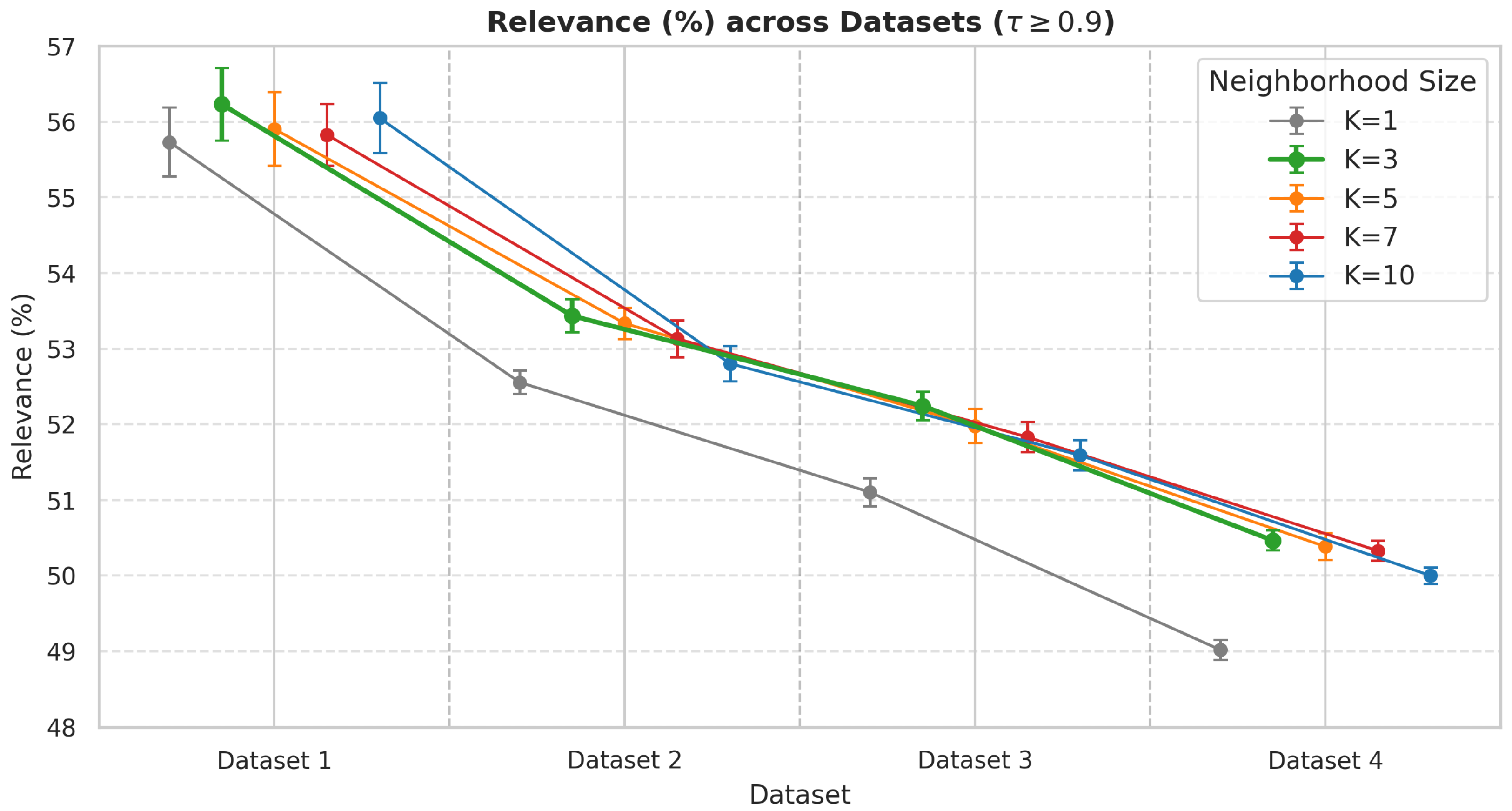
Nevertheless, the consistent $AAR(\%)$$\ge 50\%$ at high thresholds ($\tau \ge 0.9$) demonstrates the efficacy of the proposed emotional collaborative filtering approach in providing recommendations that are highly aligned with the user’s emotional profile.

Regarding the neighborhood size $Top-K$, the results indicate that $Top-K=1$ consistently produces the lowest $AAR$. This is expected because the system’s reliance on a single most similar user limits the candidate pool, frequently forcing the inclusion of non-affective aligned items. The same phenomenon is further evidenced by the $RDA$ results. Conversely, increasing $Top-K$ expands the candidate set, facilitating more robust aggregation of preferences from a wider spectrum of similar users, thereby increasing the probability of identifying items with greater affective alignment.

Notably, at high thresholds ($\tau \ge 0.9$), the $AAR$ values across all neighborhood sizes ($Top-K\in \{1,3,5,7,10\}$) plateau within overlapping standard deviations across all datasets. This indicates that affective recommendation alignment is robust to neighborhood size under strict emotional constraints.

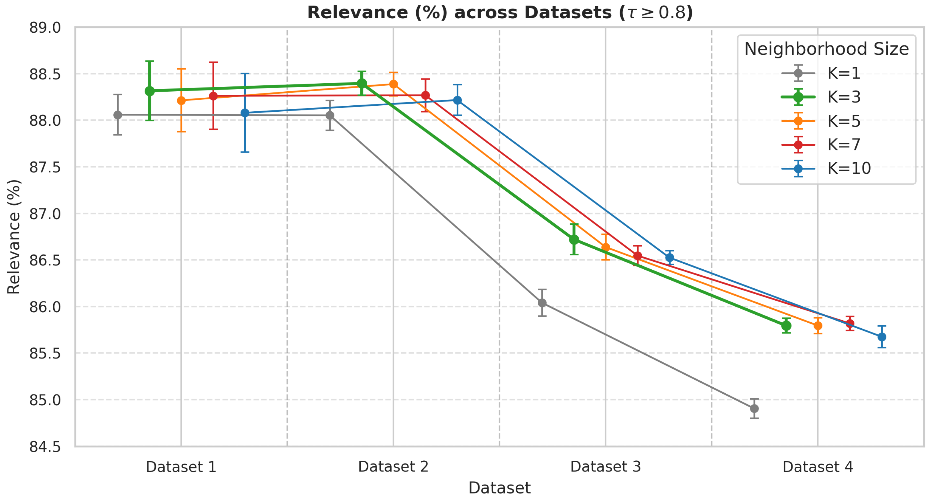
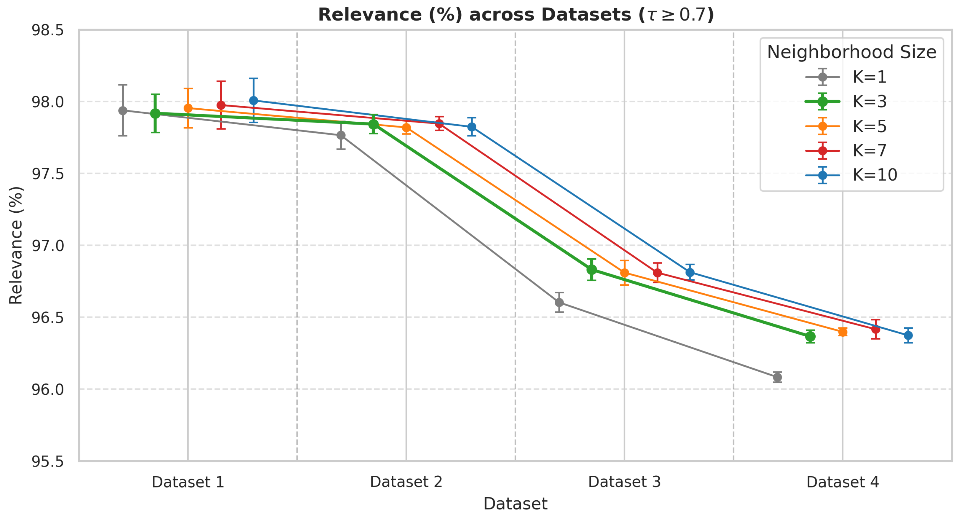
In order to better visualize the trade-offs across neighborhood sizes and threshold levels, we plot the average $AAR$ scores alongside their standard deviation intervals in Figure 1, Figure 2 and Figure 3 (corresponding to $\tau \in \{0.7,0.8,0.9\}$). As illustrated by the prominent green trajectory, our empirical evaluation reveals that $Top-K=3$ achieves the highest $AAR$ score most frequently across the datasets and $\tau$ thresholds, closely followed by $Top-K=5$. Consequently, we identify $Top-K=3$ as an effective neighborhood parameter that maintains stable performance levels while operating within a narrow and high-fidelity user cluster. This configuration provides sufficient information for targeted recommendations without expanding into larger neighborhood sizes that risk noise dilution. These visual and numerical findings reveal that a narrow $Top-K=3$ neighborhood maintains greater affective recommendation alignment, as restricting aggregation to the three most similar users minimizes the noise and dilution of affective alignment that is associated with broader neighborhoods.

4.3.4. Statistical Analysis

To rigorously evaluate the trade-offs across neighborhood sizes, we conduct two-sided paired significance tests comparing the baseline $Top-K=3$ configuration against alternative configurations ($Top-K\in \{1,5,7,10\}$) across all datasets, iterations, and similarity thresholds ($\tau$), with the results shown in

Table 5. Pairwise statistical comparisons between baseline $Top-K=3$ and alternative $Top-K\in \{1,5,7,10\}$ configurations across datasets and $\tau$ thresholds. Each cell displays the mean difference ($\Delta ={\overline{X}}_{Top-K=3}-{\overline{X}}_{Top-K}$), unadjusted $95\%$ confidence interval $[{\mathrm{CI}}_{\mathrm{lower}},{\mathrm{CI}}_{\mathrm{upper}}]$, and Holm–Bonferroni adjusted p-value ($p_{\mathrm{adj}}$) from paired t-tests (Monte Carlo cross-validation $N=10$ iterations). p-value corrections are calculated independently per dataset. Cells highlighted in green indicate statistical significance ($p_{\mathrm{adj}}<0.05$), while orange indicates moderate significance statistical significance ($0.05\le p_{\mathrm{adj}}<0.10$) and red indicates non-significance ($p_{\mathrm{adj}}\ge 0.10$). A positive $\Delta$ indicates that baseline $Top-K=3$ achieved higher affective alignment than the comparison configuration. $NA$ indicates configurations with perfect scores (100% Affective Alignment Rate) across all iterations, making paired testing uncomputable.

Dataset	K	$\mathit{\tau }=0.5$	$\mathit{\tau }=0.6$	$\mathit{\tau }=0.7$	$\mathit{\tau }=0.8$	$\mathit{\tau }=0.9$
Dataset 1	1	$NA$	$-0.005$ $[-0.027,0.018]$ ($p_{\mathrm{adj}}=1.000$)	$-0.020$ $[-0.162,0.122]$ ($p_{\mathrm{adj}}=1.000$)	$+0.256$ $[0.023,0.489]$ ($p_{\mathrm{adj}}=0.485$)	$+0.499$ $[0.135,0.862]$ ($p_{\mathrm{adj}}=0.203$)
	5	$NA$	$-0.006$ $[-0.046,0.034]$ ($p_{\mathrm{adj}}=1.000$)	$-0.036$ $[-0.150,0.079]$ ($p_{\mathrm{adj}}=1.000$)	$+0.102$ $[-0.174,0.378]$ ($p_{\mathrm{adj}}=1.000$)	$+0.326$ $[0.082,0.570]$ ($p_{\mathrm{adj}}=0.215$)
	7	$NA$	$-0.011$ $[-0.049,0.028]$ ($p_{\mathrm{adj}}=1.000$)	$-0.057$ $[-0.181,0.067]$ ($p_{\mathrm{adj}}=1.000$)	$+0.053$ $[-0.267,0.373]$ ($p_{\mathrm{adj}}=1.000$)	$+0.402$ $[0.010,0.795]$ ($p_{\mathrm{adj}}=0.553$)
	10	$NA$	$+0.030$ $[-0.014,0.074]$ ($p_{\mathrm{adj}}=1.000$)	$-0.089$ $[-0.174,-0.004]$ ($p_{\mathrm{adj}}=0.553$)	$+0.236$ $[-0.149,0.620]$ ($p_{\mathrm{adj}}=1.000$)	$+0.180$ $[-0.067,0.428]$ ($p_{\mathrm{adj}}=1.000$)
Dataset 2	1	$-0.004$ $[-0.010,0.003]$ ($p_{\mathrm{adj}}=1.000$)	$+0.015$ $[-0.008,0.038]$ ($p_{\mathrm{adj}}=1.000$)	$+0.078$ $[0.002,0.153]$ ($p_{\mathrm{adj}}=0.627$)	$+0.343$ $[0.192,0.493]$ ($p_{\mathrm{adj}}=0.010$)	$+0.878$ $[0.731,1.025]$ ($p_{\mathrm{adj}}<0.001$)
	5	$-0.006$ $[-0.013,0.000]$ ($p_{\mathrm{adj}}=0.634$)	$-0.018$ $[-0.035,-0.002]$ ($p_{\mathrm{adj}}=0.524$)	$+0.023$ $[-0.033,0.079]$ ($p_{\mathrm{adj}}=1.000$)	$+0.008$ $[-0.137,0.152]$ ($p_{\mathrm{adj}}=1.000$)	$+0.101$ $[-0.076,0.277]$ ($p_{\mathrm{adj}}=1.000$)
	7	$-0.008$ $[-0.015,-0.000]$ ($p_{\mathrm{adj}}=0.634$)	$-0.005$ $[-0.029,0.020]$ ($p_{\mathrm{adj}}=1.000$)	$-0.003$ $[-0.070,0.064]$ ($p_{\mathrm{adj}}=1.000$)	$+0.127$ $[-0.044,0.299]$ ($p_{\mathrm{adj}}=1.000$)	$+0.303$ $[0.175,0.430]$ ($p_{\mathrm{adj}}=0.008$)
	10	$-0.003$ $[-0.011,0.004]$ ($p_{\mathrm{adj}}=1.000$)	$-0.008$ $[-0.029,0.014]$ ($p_{\mathrm{adj}}=1.000$)	$+0.019$ $[-0.026,0.064]$ ($p_{\mathrm{adj}}=1.000$)	$+0.179$ $[0.052,0.305]$ ($p_{\mathrm{adj}}=0.173$)	$+0.631$ $[0.533,0.729]$ ($p_{\mathrm{adj}}<0.001$)
Dataset 3	1	$+0.019$ $[0.009,0.030]$ ($p_{\mathrm{adj}}=0.038$)	$+0.051$ $[0.029,0.072]$ ($p_{\mathrm{adj}}=0.006$)	$+0.228$ $[0.169,0.287]$ ($p_{\mathrm{adj}}<0.001$)	$+0.681$ $[0.534,0.828]$ ($p_{\mathrm{adj}}<0.001$)	$+1.142$ $[1.016,1.268]$ ($p_{\mathrm{adj}}<0.001$)
	5	$-0.004$ $[-0.016,0.008]$ ($p_{\mathrm{adj}}=1.000$)	$-0.026$ $[-0.062,0.010]$ ($p_{\mathrm{adj}}=1.000$)	$+0.021$ $[-0.026,0.069]$ ($p_{\mathrm{adj}}=1.000$)	$+0.083$ $[-0.070,0.236]$ ($p_{\mathrm{adj}}=1.000$)	$+0.268$ $[0.098,0.438]$ ($p_{\mathrm{adj}}=0.067$)
	7	$-0.004$ $[-0.016,0.008]$ ($p_{\mathrm{adj}}=1.000$)	$+0.002$ $[-0.023,0.028]$ ($p_{\mathrm{adj}}=1.000$)	$+0.021$ $[-0.046,0.089]$ ($p_{\mathrm{adj}}=1.000$)	$+0.174$ $[0.054,0.295]$ ($p_{\mathrm{adj}}=0.095$)	$+0.414$ $[0.301,0.527]$ ($p_{\mathrm{adj}}<0.001$)
	10	$-0.009$ $[-0.014,-0.005]$ ($p_{\mathrm{adj}}=0.015$)	$-0.005$ $[-0.033,0.023]$ ($p_{\mathrm{adj}}=1.000$)	$+0.018$ $[-0.050,0.087]$ ($p_{\mathrm{adj}}=1.000$)	$+0.195$ $[0.074,0.316]$ ($p_{\mathrm{adj}}=0.063$)	$+0.654$ $[0.532,0.777]$ ($p_{\mathrm{adj}}<0.001$)
Dataset 4	1	$+0.016$ $[0.004,0.029]$ ($p_{\mathrm{adj}}=0.230$)	$+0.067$ $[0.043,0.090]$ ($p_{\mathrm{adj}}=0.002$)	$+0.284$ $[0.254,0.313]$ ($p_{\mathrm{adj}}<0.001$)	$+0.891$ $[0.806,0.975]$ ($p_{\mathrm{adj}}<0.001$)	$+1.445$ $[1.314,1.576]$ ($p_{\mathrm{adj}}<0.001$)
	5	$-0.009$ $[-0.020,0.002]$ ($p_{\mathrm{adj}}=0.789$)	$-0.010$ $[-0.034,0.015]$ ($p_{\mathrm{adj}}=1.000$)	$-0.031$ $[-0.063,0.000]$ ($p_{\mathrm{adj}}=0.530$)	$+0.000$ $[-0.045,0.046]$ ($p_{\mathrm{adj}}=1.000$)	$+0.081$ $[-0.057,0.219]$ ($p_{\mathrm{adj}}=1.000$)
	7	$-0.011$ $[-0.025,0.003]$ ($p_{\mathrm{adj}}=0.789$)	$-0.018$ $[-0.044,0.008]$ ($p_{\mathrm{adj}}=0.945$)	$-0.049$ $[-0.091,-0.008]$ ($p_{\mathrm{adj}}=0.313$)	$-0.023$ $[-0.085,0.039]$ ($p_{\mathrm{adj}}=1.000$)	$+0.136$ $[0.004,0.268]$ ($p_{\mathrm{adj}}=0.489$)
	10	$-0.017$ $[-0.027,-0.006]$ ($p_{\mathrm{adj}}=0.091$)	$-0.017$ $[-0.034,0.001]$ ($p_{\mathrm{adj}}=0.558$)	$-0.007$ $[-0.046,0.033]$ ($p_{\mathrm{adj}}=1.000$)	$+0.119$ $[0.012,0.226]$ ($p_{\mathrm{adj}}=0.401$)	$+0.464$ $[0.313,0.615]$ ($p_{\mathrm{adj}}=0.001$)

. The $NA$ values indicate configurations in which both $Top-K=3$ and alternative configurations achieved 100% Affective Alignment Rate across all iterations, resulting in an undefined paired test.

For each pairwise test, the null hypothesis ($H_0$) states that there is no difference in mean performance between $Top-K=3$ and alternative configurations ($H_0:{\mu }_{op-K=3}-{\mu }_{Top-K}=0$), while the alternative hypothesis ($H_1$) states that a significant difference exists ($H_1:{\mu }_{op-K=3}-{\mu }_{Top-K}\ne 0$). The unit of analysis is the mean Affective Alignment Rate score per iteration. To satisfy the paired-sample requirement, the exact same $N=10$ Monte Carlo cross-validation data partitions were evaluated across all $Top-K$ configurations. Approximate normality of the paired differences ($\Delta =X_{Top-K=3}-X_{Top-K}$) was confirmed using Shapiro–Wilk tests ($\alpha =0.05$). To control the family-wise error rates, p-values were adjusted using the Holm–Bonferroni procedure applied independently within each experimental dataset ($p_{\mathrm{adj}}$). The reported 95% confidence intervals are unadjusted for multiple testing in order to reflect sample-level precision. All statistical tests, multiple testing corrections, $95\%$ confidence intervals, and effect size calculations were executed in Python (v3.12.13) using scipy.stats (v1.16.3) and statsmodels (v0.14.6).

As illustrated by the performance trends and confirmed by our statistical analysis, $Top-K=3$ frequently establishes itself as a competitive parameter. Specifically, at stricter thresholds ($\tau \ge 0.8$ and $0.9$), pairwise comparisons confirm that $Top-K=3$ yields statistically significant improvements ($p<0.05$, highlighted in green in Table 5), especially on larger size datasets. While certain configurations show statistically indistinguishable performance ($p\ge 0.05$, shown in red), $Top-K=3$ is consistently shown to be an effective parameter at the highest thresholds $\tau$.

4.3.5. Comparative Analysis Against Non-Emotional Baselines

To evaluate whether emotional representations enhance affective alignment compared to non-emotional recommendation mechanisms, we benchmark the $Top-K=3$ affective model against three non-emotional baselines:

• Popularity-based recommendation: Selects globally popular items regardless of affective user history.
• Random recommendation: Uniformly selects items across the item space.
• Genre-based recommendation: Leverages non-emotional structural item metadata (genres).

All models were evaluated across the experimental datasets and affective strictness thresholds ($\tau \in \{0.5,0.6,0.7,0.8,0.9\}$) using Affective Alignment Rate ($AAR$) as the evaluation measure.

Table 6. Comparisons of Affective Alignment Rate $AAR$ (%) (average values per ten iterations ± standard deviation) between $Top-K=3$ and baselines (Popularity, Random, and Genre) across datasets and $\tau$ thresholds.

Dataset	Method	$\mathit{\tau }\ge 0.5$	$\mathit{\tau }\ge 0.6$	$\mathit{\tau }\ge 0.7$	$\mathit{\tau }\ge 0.8$	$\mathit{\tau }\ge 0.9$
Dataset 1	$Top-K=3$	100.0 ± 0.0	99.9 ± 0.0	97.9 ± 0.1	88.3 ± 0.3	56.2 ± 0.5
	Popularity	100.0 ± 0.0	99.6 ± 0.0	96.0 ± 0.0	71.5 ± 0.0	32.6 ± 0.0
	Random	100.0 ± 0.0	99.9 ± 0.0	97.9 ± 0.1	87.4 ± 0.2	54.2 ± 0.3
	Genres	100.0 ± 0.0	100.0 ± 0.0	99.4 ± 0.0	91.8 ± 0.2	71.1 ± 0.2
Dataset 2	$Top-K=3$	100.0 ± 0.0	99.7 ± 0.0	97.8 ± 0.1	88.4 ± 0.1	53.4 ± 0.2
	Popularity	100.0 ± 0.0	99.7 ± 0.0	97.6 ± 0.0	87.2 ± 0.0	50.3 ± 0.0
	Random	100.0 ± 0.0	99.6 ± 0.0	97.3 ± 0.1	86.1 ± 0.1	47.8 ± 0.2
	Genres	100.0 ± 0.0	99.9 ± 0.0	99.0 ± 0.0	93.8 ± 0.1	70.1 ± 0.2
Dataset 3	$Top-K=3$	99.9 ± 0.0	99.2 ± 0.0	96.8 ± 0.1	86.7 ± 0.2	52.2 ± 0.2
	Popularity	100.0 ± 0.0	99.5 ± 0.0	97.5 ± 0.0	86.9 ± 0.0	44.4 ± 0.0
	Random	99.8 ± 0.0	99.0 ± 0.0	95.7 ± 0.1	83.3 ± 0.1	45.6 ± 0.2
	Genres	100.0 ± 0.0	99.7 ± 0.0	98.1 ± 0.1	91.3 ± 0.1	66.3 ± 0.1
Dataset 4	$Top-K=3$	99.8 ± 0.0	99.1 ± 0.0	96.4 ± 0.0	85.8 ± 0.1	50.5 ± 0.1
	Popularity	99.9 ± 0.0	99.3 ± 0.0	96.2 ± 0.0	75.0 ± 0.0	32.9 ± 0.0
	Random	99.8 ± 0.0	98.8 ± 0.0	95.0 ± 0.0	81.3 ± 0.1	42.1 ± 0.1
	Genres	100.0 ± 0.0	99.7 ± 0.0	98.3 ± 0.0	91.8 ± 0.1	67.1 ± 0.1

and

Table 7. Pairwise statistical comparisons between $Top-K=3$ and baselines (Popularity, Random, and Genre) across datasets and $\tau$ thresholds. Each cell displays the mean difference ($\Delta ={\overline{X}}_{Top-K=3}-{\overline{X}}_{baseline}$), $95\%$ confidence interval $[{\mathrm{CI}}_{\mathrm{lower}},{\mathrm{CI}}_{\mathrm{upper}}]$, and Holm–Bonferroni adjusted p-value ($p_{\mathrm{adj}}$) from paired t-tests (Monte Carlo cross-validation $N=10$ iterations). Cells highlighted in green indicate that $Top-K=3$ performed significantly better ($\Delta >0,p_{\mathrm{adj}}<0.05$), red indicates that $Top-K=3$ performed significantly worse ($\Delta <0,p_{\mathrm{adj}}<0.05$), and gray indicates no statistically significant difference ($p_{\mathrm{adj}}\ge 0.05$). $NA$ indicates configurations with perfect scores across all iterations, making paired testing uncomputable.

Dataset	Method	$\mathit{\tau }=0.5$	$\mathit{\tau }=0.6$	$\mathit{\tau }=0.7$	$\mathit{\tau }=0.8$	$\mathit{\tau }=0.9$
Dataset 1	Popularity	$NA$	$+0.224$ $[0.195,0.252]$ ($p_{\mathrm{adj}}<0.001$)	$+1.898$ $[1.801,1.996]$ ($p_{\mathrm{adj}}<0.001$)	$+16.790$ $[16.574,17.007]$ ($p_{\mathrm{adj}}<0.001$)	$+23.588$ $[23.227,23.949]$ ($p_{\mathrm{adj}}<0.001$)
	Random	$NA$	$-0.017$ $[-0.057,0.023]$ ($p_{\mathrm{adj}}=0.735$)	$-0.003$ $[-0.143,0.137]$ ($p_{\mathrm{adj}}=0.962$)	$+0.908$ $[0.619,1.197]$ ($p_{\mathrm{adj}}<0.001$)	$+2.051$ $[1.636,2.466]$ ($p_{\mathrm{adj}}<0.001$)
	Genres	$NA$	$-0.136$ $[-0.166,-0.105]$ ($p_{\mathrm{adj}}<0.001$)	$-1.482$ $[-1.581,-1.383]$ ($p_{\mathrm{adj}}<0.001$)	$-3.521$ $[-3.712,-3.330]$ ($p_{\mathrm{adj}}<0.001$)	$-14.916$ $[-15.312,-14.521]$ ($p_{\mathrm{adj}}<0.001$)
Dataset 2	Popularity	$-0.021$ $[-0.025,-0.016]$ ($p_{\mathrm{adj}}<0.001$)	$-0.084$ $[-0.101,-0.068]$ ($p_{\mathrm{adj}}<0.001$)	$+0.221$ $[0.172,0.270]$ ($p_{\mathrm{adj}}<0.001$)	$+1.155$ $[1.059,1.250]$ ($p_{\mathrm{adj}}<0.001$)	$+3.140$ $[2.978,3.303]$ ($p_{\mathrm{adj}}<0.001$)
	Random	$+0.009$ $[0.003,0.016]$ ($p_{\mathrm{adj}}=0.032$)	$+0.104$ $[0.085,0.122]$ ($p_{\mathrm{adj}}<0.001$)	$+0.540$ $[0.475,0.606]$ ($p_{\mathrm{adj}}<0.001$)	$+2.315$ $[2.214,2.416]$ ($p_{\mathrm{adj}}<0.001$)	$+5.679$ $[5.444,5.913]$ ($p_{\mathrm{adj}}<0.001$)
	Genres	$-0.020$ $[-0.024,-0.016]$ ($p_{\mathrm{adj}}<0.001$)	$-0.249$ $[-0.271,-0.228]$ ($p_{\mathrm{adj}}<0.001$)	$-1.142$ $[-1.199,-1.085]$ ($p_{\mathrm{adj}}<0.001$)	$-5.358$ $[-5.439,-5.276]$ ($p_{\mathrm{adj}}<0.001$)	$-16.636$ $[-16.844,-16.428]$ ($p_{\mathrm{adj}}<0.001$)
Dataset 3	Popularity	$-0.055$ $[-0.065,-0.044]$ ($p_{\mathrm{adj}}<0.001$)	$-0.316$ $[-0.339,-0.294]$ ($p_{\mathrm{adj}}<0.001$)	$-0.675$ $[-0.728,-0.622]$ ($p_{\mathrm{adj}}<0.001$)	$-0.160$ $[-0.280,-0.041]$ ($p_{\mathrm{adj}}=0.042$)	$+7.836$ $[7.703,7.970]$ ($p_{\mathrm{adj}}<0.001$)
	Random	$+0.088$ $[0.073,0.102]$ ($p_{\mathrm{adj}}<0.001$)	$+0.263$ $[0.227,0.298]$ ($p_{\mathrm{adj}}<0.001$)	$+1.088$ $[1.021,1.155]$ ($p_{\mathrm{adj}}<0.001$)	$+3.413$ $[3.252,3.574]$ ($p_{\mathrm{adj}}<0.001$)	$+6.661$ $[6.479,6.843]$ ($p_{\mathrm{adj}}<0.001$)
	Genres	$-0.057$ $[-0.069,-0.045]$ ($p_{\mathrm{adj}}<0.001$)	$-0.469$ $[-0.490,-0.449]$ ($p_{\mathrm{adj}}<0.001$)	$-1.301$ $[-1.351,-1.252]$ ($p_{\mathrm{adj}}<0.001$)	$-4.588$ $[-4.702,-4.474]$ ($p_{\mathrm{adj}}<0.001$)	$-14.033$ $[-14.147,-13.919]$ ($p_{\mathrm{adj}}<0.001$)
Dataset 4	Popularity	$-0.080$ $[-0.088,-0.073]$ ($p_{\mathrm{adj}}<0.001$)	$-0.227$ $[-0.246,-0.208]$ ($p_{\mathrm{adj}}<0.001$)	$+0.212$ $[0.180,0.245]$ ($p_{\mathrm{adj}}<0.001$)	$+10.773$ $[10.714,10.831]$ ($p_{\mathrm{adj}}<0.001$)	$+17.575$ $[17.478,17.673]$ ($p_{\mathrm{adj}}<0.001$)
	Random	$+0.055$ $[0.044,0.067]$ ($p_{\mathrm{adj}}<0.001$)	$+0.286$ $[0.261,0.311]$ ($p_{\mathrm{adj}}<0.001$)	$+1.415$ $[1.373,1.458]$ ($p_{\mathrm{adj}}<0.001$)	$+4.518$ $[4.421,4.614]$ ($p_{\mathrm{adj}}<0.001$)	$+8.356$ $[8.225,8.488]$ ($p_{\mathrm{adj}}<0.001$)
	Genres	$-0.143$ $[-0.150,-0.135]$ ($p_{\mathrm{adj}}<0.001$)	$-0.586$ $[-0.607,-0.564]$ ($p_{\mathrm{adj}}<0.001$)	$-1.906$ $[-1.948,-1.865]$ ($p_{\mathrm{adj}}<0.001$)	$-5.960$ $[-6.033,-5.888]$ ($p_{\mathrm{adj}}<0.001$)	$-16.658$ $[-16.770,-16.546]$ ($p_{\mathrm{adj}}<0.001$)

report the $AAR$ values and statistical pairwise comparisons using paired t-tests with Holm–Bonferroni correction ($N=10$ Monte Carlo iterations).

$Top-K=3$ demonstrates statistically significant superiority ($p_{\mathrm{adj}}<0.001$) over the Random baseline across nearly all thresholds and datasets, reaching performance gains up to $\Delta =+8.356$ at $\tau =0.9$. When compared against the Popularity baseline, $Top-K=3$ yields affective alignment gains at stricter thresholds ($\tau \ge 0.7$), outperforming Popularity by up to $\Delta =+23.588$ on Dataset 1 ($p_{\mathrm{adj}}<0.001$). At lower strictness thresholds ($\tau \le 0.6$), Popularity achieves slight superiority, reflecting that broadly popular items cover wide emotional baselines when affective constraints are loose.

While the naive non-emotional baselines (Random and Popularity) drop sharply in $AAR$ as $\tau$ increases, $Top-K=3$ maintains significantly higher $AAR$ scores at medium-to-high strictness levels ($\tau \ge 0.7$). This proves that explicit emotional modeling does not merely filter items to satisfy affective criteria arbitrarily; rather, it identifies items that have both affective alignment and relevance to the user.

Comparison against the Genre baseline reveals a nuanced trade-off: while $Top-K=3$ reliably outpaces the naive heuristics, the non-emotional Genre baseline achieves higher raw alignment scores across all configurations ($\Delta <0,p_{\mathrm{adj}}<0.001$). This indicates that coarse metadata categories (book genres) naturally encode implicit affective clusters, serving as a highly competitive non-emotional proxy.

4.3.6. Comparative Analysis Against Prior Work

We further compare the proposed collaborative filtering system against prior work [11], utilizing the exact same dataset to evaluate the trade-offs between content-based and collaborative filtering in terms of catalog coverage. In addition, a comparison using Dataset 3 and the collaborative filtering technique considers both single-source Goodreads reviews (SS) and multi-source Goodreads and Amazon reviews (MS) [12].

The evaluation of catalog coverage against [11] reveals a distinct divergence between the two paradigms as the dataset size increases. While the content-based approach exhibits a clear decay in coverage, dropping from 95% to 84% as the dataset size increases, the collaborative filtering algorithm maintains robust 100% coverage across all test tiers. However, this high coverage is partly sustained by the algorithm’s fallback mechanism, which introduces randomized item selection to handle sparse recommendation pools. Consequently, while content-based filtering becomes progressively constrained to a concentrated subset of items, the collaborative filtering results should be interpreted with consideration of this fallback behavior.

Next, to assess the structural behavior and exploration capabilities of our algorithm, we compare its Randomness-Degree Assessment against prior benchmarks established in [12].

A comparison of our current findings with the results presented in [12] demonstrates an improvement in the system’s ability to generate personalized recommendations. While [12] reported that multi-source reviews achieved a $GRL$ of $81\%$, with stochastic fallback rates of $5\%$ ($RF$) and $14\%$ ($FR$), respectively, our current model presents higher affective alignment scores under larger neighborhood size configurations. Specifically, by increasing the neighborhood size to $Top-K=10$, we observe an increase in $GRL$ to $84\%$, accompanied by a reduction in stochastic fallback to $3\%$ for $RF$ and $13\%$ for $FR$. These results suggest that optimizing the neighborhood size ($Top-K$) effectively leverages the available data to enhance personalized recommendations beyond the limits identified in previous work.

5. Conclusions

In this contribution, we present an emotion-aware collaborative filtering framework designed to capture the latent affective dimensions of reading by extracting emotional embedding spaces from social media reviews. Unlike traditional metadata models, in this system the similarity between users is computed exclusively based on the emotions they share with respect to the same book(s). To validate the proposed framework, we conduct a neighborhood size sensitivity analysis alongside extensive evaluations across four book datasets of varying sizes collected from the Goodreads website.

With respect to RQ1, our systematic evaluations demonstrate that recommendation affective alignment varies dynamically and predictably with neighborhood size ($Top-K\in \{1,3,5,7,10\}$) when relying solely on affective embeddings. The results confirm that calculating user similarity from emotional text data provides a structurally sound signal for collaborative filtering pipelines.

For RQ2, our neighborhood size sensitivity analysis identifies $Top-K=3$ as an effective neighborhood parameter. This tightly constrained cluster size successfully balances acquisition of candidate users with affective alignment against mitigation of the semantic noise introduced by larger neighborhoods with lower affective alignment.

Finally, for RQ3, the evaluation demonstrates that the framework maintains high affective recommendation alignment even under stringent emotional similarity thresholds ($\tau$). At high thresholds ($\tau \ge 0.9$), the Affective Alignment Rate values across all neighborhood sizes ($Top-K\in \{1,3,5,7,10\}$) plateau within overlapping standard deviations across experimental datasets. Notably, $Top-K=3$ achieves the highest $AAR$ score most frequently across datasets and $\tau$ levels, closely followed by $Top-K=5$. This identifies $Top-K=3$ as an effective neighborhood parameter that maintains stable performance levels while operating within a narrow high-fidelity user cluster. Moreover, when comparing the results with former experiments utilizing multi-source reviews, we observe an increase in personalized recommendations ($GRL$) from the previously reported $81\%$ to $84\%$, alongside a decrease in stochastic fallback rates. This indicates that these neighborhood dimensions can effectively leverage data depth even beneath strict thresholds.

While the proposed framework demonstrates robust stability and adaptability under stringent threshold constraints, several pathways remain for future exploration. Moving forward, we intend to expand our experimental studies to evaluate the system’s sensitivity across different recommendation list lengths ($nREC$). Additionally, we plan to broaden our evaluation framework to measure further metrics, specifically focusing on how neighborhood adjustments affect the diversity and novelty of the recommended items.

References

1. Hossein Arabi, V.B.; Shuib, N.L.M. A Context-Aware Personalized Hybrid Book Recommender System. J. Web Eng. 2020, 19, 405–428. [Google Scholar] [CrossRef] [Scilit]
2. Alatrash, R.; Priyadarshini, R. Fine-grained Sentiment-enhanced Collaborative Filtering-based Hybrid Recommender System. J. Web Eng. 2023, 22, 983–1036. [Google Scholar] [CrossRef] [Scilit]
3. Tamada, T.; Saga, R. Book Recommender System Using CNN Capturing Feature of Synopses and Reviews. In Proceedings of the HCI International 2022–Late Breaking Papers: Interacting with eXtended Reality and Artificial Intelligence; Chen, J.Y.C., Fragomeni, G., Degen, H., Ntoa, S., Eds.; Springer: Cham, Switzerland, 2022; pp. 518–530. [Google Scholar] [CrossRef] [Scilit]
4. Qian, Y.; Zhang, Y.; Ma, X.; Yu, H.; Peng, L. EARS: Emotion-aware recommender system based on hybrid information fusion. Inf. Fusion 2019, 46, 141–146. [Google Scholar] [CrossRef] [Scilit]
5. Devlin, J.; Chang, M.W.; Lee, K.; Toutanova, K. BERT: Pre-training of Deep Bidirectional Transformers for Language Understanding. In Proceedings of the 2019 Conference of the North American Chapter of the Association for Computational Linguistics: Human Language Technologies, Volume 1 (Long and Short Papers); ACL: Stroudsburg, PA, USA, 2019; pp. 4171–4186. [Google Scholar] [CrossRef] [Scilit]
6. Vaswani, A.; Shazeer, N.; Parmar, N.; Uszkoreit, J.; Jones, L.; Gomez, A.N.; Kaiser, Ł.; Polosukhin, I. Attention is All you Need. In Proceedings of the NIPS’17: Proceedings of the 31st International Conference on Neural Information Processing Systems; Curran Associates, Inc.: Red Hook, NY, USA, 2017; pp. 6000–6010. [Google Scholar]
7. Ai, J.; Cai, Y.; Su, Z.; Peng, D.; Zhao, F. Measuring similarity based on user activeness in recommender systems to improve algorithm scalability. Eng. Appl. Artif. Intell. 2023, 126, 106842. [Google Scholar] [CrossRef] [Scilit]
8. Dokoupil, P.; Peska, L. The Effect of Similarity Metric and Group Size on Outlier Selection & Satisfaction in Group Recommender Systems. In Proceedings of the Adjunct Proceedings of the 31st ACM Conference on User Modeling, Adaptation and Personalization; ACM: New York, NY, USA, 2023; pp. 296–301. [Google Scholar] [CrossRef] [Scilit]
9. Kim, T.Y.; Ko, H.; Kim, S.H.; Kim, H.D. Modeling of Recommendation System Based on Emotional Information and Collaborative Filtering. Sensors 2021, 21, 1997. [Google Scholar] [CrossRef] [Scilit] [PubMed]
10. Kweon, W.; Kang, S.; Jang, S.; Yu, H. Top-Personalized-K Recommendation. In Proceedings of the ACM Web Conference 2024; ACM: New York, NY, USA, 2024; pp. 3388–3399. [Google Scholar] [CrossRef] [Scilit]
11. Luțan, E.R.; Bădică, C. Systematic Features Selection in Content-Based Filtering Books Recommender System. In Proceedings of the 2025 IEEE International Conference on Systems, Man, and Cybernetics (SMC); IEEE: Piscataway, NJ, USA, 2025; pp. 6708–6713. [Google Scholar] [CrossRef] [Scilit]
12. Luţan, E.R.; Bădică, C. Literature Books Recommender System using Collaborative Filtering and Multi-Source Reviews. In Proceedings of the 19th Conference on Computer Science and Intelligence Systems FedCSIS 2024; Polish Information Processing Society: Warsaw, Poland, 2024; pp. 225–230. [Google Scholar] [CrossRef] [Scilit]
13. Karabila, I.; Darraz, N.; El-Ansari, A.; Alami, N.; El Mallahi, M. Enhancing Collaborative Filtering-Based Recommender System Using Sentiment Analysis. Future Internet 2023, 15, 235. [Google Scholar] [CrossRef] [Scilit]
14. Sun, Y.; Liu, Q. Collaborative filtering recommendation based on K-nearest neighbor and non-negative matrix factorization algorithm. J. Supercomput. 2024, 81, 79. [Google Scholar] [CrossRef] [Scilit]
15. Liu, D.; Yang, C.; Tang, X.; Wang, Y.; Lyu, F.; Luo, W.; He, X.; Ming, Z.; Zhao, X. MultiFS: Automated Multi-Scenario Feature Selection in Deep Recommender Systems. In Proceedings of the 17th ACM International Conference on Web Search and Data Mining; ACM: New York, NY, USA, 2024; pp. 434–442. [Google Scholar] [CrossRef] [Scilit]
16. Yan, T.; Cao, L.; Chai, P.; Yu, S. Improving collaborative filtering with SNE–GCN: A second-order neighbor enhanced graph convolutional network. Multimed. Syst. 2024, 30, 160. [Google Scholar] [CrossRef] [Scilit]
17. Koohi, H.; Kiani, K. A new method to find neighbor users that improves the performance of Collaborative Filtering. Expert Syst. Appl. 2017, 83, 30–39. [Google Scholar] [CrossRef] [Scilit]
18. Subramaniyaswamy, V.; Logesh, R. Adaptive KNN based Recommender System through Mining of User Preferences. Wirel. Pers. Commun. 2017, 97, 2229–2247. [Google Scholar] [CrossRef] [Scilit]
19. Airen, S.; Agrawal, J. Movie Recommender System Using K-Nearest Neighbors Variants. Natl. Acad. Sci. Lett. 2022, 45, 75–82. [Google Scholar] [CrossRef] [Scilit]
20. Kim, M.J.; Cho, Y. Imputation of missing values in well log data using k-nearest neighbor collaborative filtering. Comput. Geosci. 2024, 193, 105712. [Google Scholar] [CrossRef] [Scilit]
21. DeRose, S.J. The Compass DeRose Guide to Emotion Words. 2005. Available online: http://www.derose.net/derose/steve/resources/emotionwords/ewords.html (accessed on 10 June 2026).
22. Citron, F.M.M.; Weekes, B.S.; Ferstl, E.C. How are affective word ratings related to lexicosemantic properties? Evidence from the Sussex Affective Word List. Appl. Psycholinguist. 2014, 35, 313–331. [Google Scholar] [CrossRef] [Scilit]
23. Årup Nielsen, F. A New ANEW: Evaluation of a Word List for Sentiment Analysis in Microblogs. In Proceedings of the ESWC2011 Workshop on ‘Making Sense of Microposts’: Big Things Come in Small Packages; Cornell University: Ithaca, NY, USA, 2011; pp. 93–98. [Google Scholar]
Figure 1. Comparison of Affective Alignment Rate ( A A R ) across datasets for τ 0.7 . The highlighted green trajectory represents T o p - K = 3 , illustrating performance relative to the considered T o p - K configurations.
Electronics 15 03710 g001
Figure 2. Comparison of Affective Alignment Rate ( A A R ) across datasets for τ 0.8 . The highlighted green trajectory represents the effective neighborhood parameter T o p - K = 3 .
Electronics 15 03710 g002
Figure 3. Comparison of Affective Alignment Rate ( A A R ) across datasets for τ 0.9 . The highlighted green trajectory represents the effective neighborhood parameter T o p - K = 3 .
Electronics 15 03710 g003