Acoustic Distance-Based System for In-Swarm Low-Cost Underwater Navigation

Abstract

This paper presents the design and simulation-based validation of an acoustic navigation system intended for operation within a swarm of underwater vehicles. The system is deployed on a mobile leader unit, while the remaining vehicles, referred to as followers, navigate relative to the leader. The proposed solution utilises two or three acoustic transmitters mounted at the front and rear, and, in the option with three transmitters, also in the middle of the leader platform. These transmitters periodically emit acoustic signals that are received by the follower vehicles. By measuring the time-of-flight of the received signals, followers estimate their distances to the transmitters. This dual(triple)-range information, combined with Kalman filter dead-reckoning, enables relative position estimation with respect to the leader, supporting coordinated swarm movement without reliance on external positioning infrastructure such as GPS, which is unavailable underwater. The system was evaluated in a simulation environment across multiple scenarios with varying levels of distance-measurement error. Rather than modelling detailed acoustic signal propagation, the study focuses on assessing the robustness of the positioning method to measurement inaccuracies. The results demonstrate that the proposed configuration provides useful relative positioning accuracy under a range of error conditions and identifies the operating conditions in which its performance deteriorates, supporting the feasibility of the proposed approach for leader–follower coordination in underwater swarms.

1. Introduction

Exploration of the underwater environment has been gaining increasing attention in recent years, driven by scientific, industrial, and environmental needs such as seabed mapping, resource exploration, infrastructure inspection, and ecosystem monitoring. Underwater vehicles play a key role in enabling these activities, especially in areas that are difficult or impossible for human divers to access. Historically, underwater operations have relied on Remotely Operated Vehicles (ROVs), which are tethered to a surface vessel and controlled by human operators. While effective, ROVs are limited by their dependence on umbilical cables and operator workload. This has led to the growing adoption of Autonomous Underwater Vehicles (AUVs), which can execute pre-programmed missions without continuous human supervision. More recently, research has increasingly focused on AUV swarms, in which multiple vehicles cooperate to perform tasks more efficiently, robustly, and at larger spatial scales than a single unit could achieve.

Navigation is a fundamental requirement for coordinated operation within a swarm of underwater vehicles, as each unit must be able to determine its position and maintain spatial relationships with others. Traditionally, underwater navigation has relied on external infrastructure, most commonly acoustic positioning systems such as Long Baseline (LBL), Short Baseline (SBL), and Ultra-Short Baseline (USBL) [1,2,3,4]. These systems provide position estimates by referencing fixed transducers deployed in the environment or mounted on surface vessels. While they can achieve high accuracy, their applicability is inherently limited to localised areas where the necessary infrastructure can be installed and maintained. Moreover, such systems are typically stationary and do not adapt to the movement of the vehicles, making them less suitable for dynamic, large-scale swarm operations that require mobility and flexibility beyond predefined operational zones.

Another class of approaches relies on onboard sensing and does not require external infrastructure. In dead-reckoning navigation [5,6], the vehicle estimates its position by integrating measurements of its own velocity, heading, and depth over time. Similarly, Simultaneous Localisation and Mapping (SLAM) techniques [7,8,9] estimate the vehicle’s position by observing and mapping features of the surrounding environment, for example, the seabed, using onboard sensors. Both approaches typically provide position estimates in a global reference frame, which can then be shared among vehicles via a communication system. However, these methods exhibit important limitations in the context of swarm operations.

In dead-reckoning, estimation errors accumulate over time, leading to drift that causes the relative positions of vehicles to diverge, making long-term coordinated operation difficult. In the case of SLAM, reliable operation requires proximity to the seabed (or other observable structures), as well as specialised sensing equipment such as multibeam echosounders, which can be costly and are not always available. Furthermore, SLAM performance depends on the presence of sufficiently distinctive environmental features, which may not exist in all operational scenarios. As a result, relying solely on global position estimates from these methods may be insufficient to maintain coherent swarm behaviour over extended periods, motivating the use of relative navigation techniques within the swarm.

In-swarm navigation can also be realised using onboard perception systems such as Forward Looking Sonar (FLS) and optical cameras [10,11,12,13,14,15], which enable vehicles to detect and localise nearby objects by estimating their bearing and range. In principle, this allows each vehicle to directly observe other members of the swarm and maintain relative positioning without relying on external infrastructure or global references. However, in practice, these approaches face significant challenges. For FLS, especially in shallow-water environments, acoustic measurements are heavily affected by reflections from the seabed and the dynamically changing water surface, as acoustic waves reflect from any boundary with a different acoustic impedance. As a result, sonar images contain numerous spurious echoes and clutter, making it difficult to reliably distinguish other vehicles from environmental features. Additionally, the detection range is limited, particularly for small, low-cost vehicles with weak acoustic signatures. When vehicles move in the same direction at similar depths, each vehicle primarily observes the rear of the preceding one, which produces only a small sonar return. Consequently, the effective FLS range is typically limited to about 15 m, and only under favourable conditions can it reach approximately 20 m. Optical cameras face even stricter limitations, as their performance strongly depends on water clarity; in turbid environments such as the Baltic Sea, the effective range is often restricted to approximately 5–7 m. These constraints significantly limit the robustness and scalability of perception-based in-swarm navigation.

To address the limitations of perception-based approaches, several acoustic relative localisation methods have been proposed for underwater multi-vehicle systems. The most common solutions rely on acoustic beaconing, in which a leader or an external beacon periodically transmits navigation signals serving as references for the remaining vehicles [16,17]. In such systems, follower vehicles are typically equipped with USBL-like receiver arrays, enabling simultaneous estimation of both the range and bearing to the acoustic source. Although these approaches provide accurate relative localisation, they require multi-element hydrophone arrays and sophisticated signal-processing algorithms, making each follower relatively expensive and limiting the scalability of large underwater swarms.

Another important class of methods is cooperative localisation, in which multiple vehicles exchange navigation information and jointly estimate their positions [2,3,18,19]. Such approaches generally improve localisation accuracy and robustness but require several vehicles to actively participate in the localisation process by transmitting acoustic messages. As a result, the acoustic communication load and energy consumption increase with the number of participating vehicles. Moreover, simultaneous acoustic transmissions may lead to packet collisions or mutual interference unless carefully coordinated using multiple-access techniques, such as time-division scheduling. Although such mechanisms can effectively prevent communication conflicts, they also increase the time required to collect measurements from all vehicles, thereby reducing the achievable localisation update rate and limiting the scalability of large underwater swarms.

Recent surveys have highlighted the growing interest in low-cost underwater swarm localisation while emphasising the need to reduce the hardware complexity of individual vehicles [20,21]. Existing USBL-based and cooperative localisation approaches provide accurate relative positioning but generally require either multi-element acoustic receiver arrays installed on each follower or active participation of multiple vehicles in the localisation process. Consequently, reducing the hardware complexity and cost of follower vehicles while preserving accurate relative localisation remains an important challenge in the development of scalable underwater swarms.

In contrast to the above approaches, this paper proposes an alternative in-swarm navigation method based on a simple acoustic system designed with cost and scalability in mind. The system is installed on a leader vehicle, which serves as a reference point for all follower units in a leader–follower configuration. It consists of only two or three acoustic transmitters mounted at the front, rear, and optionally in the middle of the leader. These transmitters periodically emit signals that are received by the followers, enabling them to estimate distances to all sources and, consequently, their relative position with respect to the leader.

A key advantage of the proposed solution is that the more complex and potentially expensive components, i.e., multiple transmitters, are located exclusively on the leader, which is unique within the swarm. In contrast, each follower is equipped with only a single, low-cost acoustic receiver, rather than a more complex USBL-like array. This significantly reduces the hardware requirements for follower vehicles, making the system more economically viable and better suited for large-scale deployments. As a result, the proposed approach offers improved scalability for applications where minimising the cost of individual swarm units is critical, while still eliminating the need for perception-based systems such as FLS or cameras.

This simplification, however, comes at the expense of localisation capability. Unlike systems equipped with hydrophone arrays, a single omnidirectional receiver cannot estimate the direction of arrival of the acoustic signal using beamforming or TDOA techniques. Consequently, follower localisation must rely exclusively on range measurements to the leader transmitters, making the achievable localisation accuracy more dependent on the relative geometry between the leader and the follower. The purpose of this work is therefore to determine whether this reduction in sensing capability still provides sufficient localisation performance for practical leader–follower swarm navigation and to identify the operating conditions under which its limitations become significant.

The main contributions of this paper are twofold. First, the paper proposes and evaluates a low-cost acoustic navigation architecture for underwater leader–follower swarms, specifically designed for inexpensive follower vehicles equipped with only a single omnidirectional hydrophone. Second, the paper systematically analyses the localisation performance of this architecture under different operating conditions, identifying both its achievable accuracy and the operational conditions under which its performance deteriorates.

It should also be emphasised that the objective of this work is not to develop a new acoustic localisation algorithm or a new state-estimation method. Instead, the proposed localisation procedure combines well-established geometric localisation and Kalman filtering within the presented navigation architecture. The research challenge addressed in this work is to determine whether the reduced sensing capability resulting from the use of a single omnidirectional hydrophone per follower still provides sufficient localisation performance for practical underwater formation keeping. Consequently, the contribution of the paper lies not in proposing a new localisation estimator, but in evaluating the trade-off between hardware simplicity, computational complexity and localisation performance, and in establishing practical design guidelines by identifying the operating conditions, geometric configurations and acoustic update intervals under which the proposed navigation architecture can be reliably employed.

Although the proposed navigation architecture relies on acoustic range measurements, a detailed underwater acoustic propagation model was intentionally omitted from the simulation framework. Instead, range measurements were represented by a stochastic error model. This simplification was adopted because the objective of this work is not to investigate the acoustic ranging subsystem itself, but to evaluate the performance of the proposed low-cost navigation architecture under different ranging accuracy conditions.

Moreover, the proposed system is intended for underwater swarms operating at relatively short inter-vehicle distances and at similar, typically shallow, depths, where the direct propagation path is expected to dominate and the influence of sound-speed stratification, ray bending, and multipath propagation is significantly reduced.

The adopted stochastic error model therefore represents the overall uncertainty of the acoustic range measurements, allowing the proposed navigation architecture to be evaluated under different ranging accuracy conditions without introducing assumptions specific to a particular underwater environment or acoustic ranging technique.

The rest of the paper is organised as follows: Section 2 specifies the proposed system, Section 3 reports the verification experiments, and the last section summarises the paper.

2. System

The system proposed in the paper, called Low-cost Acoustic In-Swarm Navigation (LAISN), is intended for a swarm of underwater vehicles organised in a leader–follower architecture. The distances between the leader and followers are small, typically less than 100 m, and the vehicles move close to the surface. The leader is a vehicle equipped with advanced navigation sensors and is responsible for guiding the swarm along a predefined trajectory toward a target location. In contrast, the follower vehicles are designed to be low-cost and equipped only with simple, less accurate sensors, such as MEMS-based inertial units, electromagnetic logs, and pressure sensors. Due to these limitations, followers can operate independently only over short distances, and for longer missions, they rely on tracking the leader.

To enable coordinated motion, followers maintain a formation defined by the leader, which may change depending on the operational scenario. For example, in cluttered environments or narrow passages, a column linear formation is preferred, while in tasks such as seabed exploration, a wider formation allows for increased coverage. Maintaining such formations requires each follower to know its position within the swarm. In the approach proposed in this paper, each follower estimates its position exclusively relative to the leader and does not rely on information about other followers. By treating the leader as a reference point, each vehicle can maintain its assigned position in the formation, defined by a desired distance and bearing relative to the leader, taking the leader’s heading into account.

The LAISN is designed to provide relative positioning of follower vehicles with respect to the leader. The leader is equipped with two or three acoustic transmitters ($N^T=2$ or 3), while each follower carries a single acoustic receiver. The transmitters are mounted at the front, rear and, in the three-transmitter configuration, at the centre of the leader. The leader periodically emits acoustic signals, each containing the transmission timestamp and information about the leader’s heading, speed, and position. Assuming time synchronisation between the leader and the followers (e.g., using high-precision clocks), each follower estimates its distances to the leader transmitters based on signal time-of-flight measurements. The follower vehicles do not participate in the acoustic localisation process as transmitters. Although they may exchange acoustic information for other purposes, such transmissions are assumed to be separated from the localisation signals in frequency, time, or by another multiple-access mechanism and therefore do not interfere with the proposed system. Consequently, mutual acoustic interference between follower vehicles is neglected.

The estimated distances are then used to determine the follower’s relative position with respect to the leader. The resulting position estimate is treated as a measurement and provided to a Kalman filter. In addition to the acoustic-based position estimate, the filter incorporates the follower’s own navigation measurements, including its speed and heading. The uncertainty associated with the acoustic position estimate is explicitly modelled and may vary depending on the measurement conditions. When this uncertainty becomes excessive, the acoustic position estimate may be down-weighted or rejected by the filter, ensuring robust and stable state estimation. Formally, the LAISN is specified below.

In the proposed system, a linear Kalman filter was deliberately selected instead of an Extended Kalman Filter in order to minimise computational complexity and facilitate implementation on inexpensive follower vehicles with limited processing resources.

2.1. Main Loop

The LAISN assumes the following evolution of the follower state:

$${\mathbf{x}}_{k|k-1}=\mathbf{A}{\mathbf{x}}_{k-1|k-1}+{\mathbf{w}}_{k-1}$$

(1)

$${\mathbf{x}}_k=\left[\begin{array}{c}{x}_k\\ y_k\\ v_{x,k}\\ v_{y,k}\end{array}\right],\mathbf{A}=\left[\begin{array}{cccc}1& 0& \Delta t& 0\\ 0& 1& 0& \Delta t\\ 0& 0& 1& 0\\ 0& 0& 0& 1\end{array}\right],{\mathbf{w}}_{k-1}\sim \mathcal{N}(\mathbf{0},\mathbf{Q}),\mathbf{Q}={\sigma }_a^2\left[\begin{array}{cccc}{\displaystyle \frac{\Delta t^4}{4}}& 0& {\displaystyle \frac{\Delta t^3}{2}}& 0\\ 0& {\displaystyle \frac{\Delta t^4}{4}}& 0& {\displaystyle \frac{\Delta t^3}{2}}\\ {\displaystyle \frac{\Delta t^3}{2}}& 0& \Delta t^2& 0\\ 0& {\displaystyle \frac{\Delta t^3}{2}}& 0& \Delta t^2\end{array}\right]$$

where $(x_k,y_k)$, $(v_{x,k},v_{y,k})$ are the position and speed of the follower at kth LAISN step, ${\sigma }_a$ is the standard deviation assigned to the unknown vehicle acceleration, and $\Delta t$ is the timestep.

The LAISN iteratively determines the follower state in three successive steps: prediction, position update, and speed update. The first step is the prediction step:

$${\widehat{\mathbf{x}}}_k^{-}=\mathbf{A}{\widehat{\mathbf{x}}}_{k-1}$$

(2)

$${\mathbf{P}}_k^{-}=\mathbf{A}{\mathbf{P}}_{k-1}{\mathbf{A}}^T+\mathbf{Q}$$

(3)

$${\mathbf{P}}_k\in {\mathbb{R}}^{4\times 4}{\mathbf{P}}_0=\left[\begin{array}{cccc}{p}_{\mathrm{pos}\text{\_}\mathrm{std}}^2& 0& 0& 0\\ 0& p_{\mathrm{pos}\text{\_}\mathrm{std}}^2& 0& 0\\ 0& 0& p_{\mathrm{vel}\text{\_}\mathrm{std}}^2& 0\\ 0& 0& 0& p_{\mathrm{vel}\text{\_}\mathrm{std}}^2\end{array}\right]$$

where $p_{\mathrm{pos}\text{\_}\mathrm{std}}$, $p_{\mathrm{vel}\text{\_}\mathrm{std}}$ are initial vehicle position and speed uncertainties, whereas ${\sigma }_a$, which is a parameter of $\mathbf{Q}$, is determined as follows:

$${\sigma }_a=\alpha ({\gamma }_v+{\gamma }_{\theta })+{\sigma }_a^0$$

(4)

where ${\sigma }_a^0$ is a predefined acceleration standard deviation, $\alpha$ is a weighting parameter, and ${\gamma }_v,{\gamma }_{\theta }\in \langle 0,1\rangle$ are coefficients describing the intensity of speed and heading changes, respectively. These coefficients are calculated independently for the leader and the follower. For each vehicle $q\in \{Leader,Follower\}$, the speed variation coefficient is determined as

$${\gamma }_v^q\left(k\right)={\displaystyle \frac{\left|v^q\left(k\right)-v^q(k-1)\right|}{v_{\max }^q}},$$

(5)

where $v^q\left(k\right)$ and $v^q(k-1)$ denote the current and previous vehicle speeds, respectively, and $v_{\max }^q$ is the maximum vehicle speed. The value used in the Kalman filter is

$${\gamma }_v\left(k\right)=\max \left\{{\gamma }_v^{Leader}\left(k\right),{\gamma }_v^{Follower}\left(k\right)\right\}.$$

(6)

Similarly, the heading variation coefficient is calculated as

$${\gamma }_{\theta }^q\left(k\right)={\displaystyle \frac{{\Delta }_{\theta }\left({\theta }^q\left(k\right),{\theta }^q(k-1)\right)}{{180}^{\circ }}},$$

(7)

where ${\Delta }_{\theta }(·,·)$ denotes the smallest absolute angular difference between two headings. The value used in the Kalman filter is

$${\gamma }_{\theta }\left(k\right)=\max \left\{{\gamma }_{\theta }^{Leader}\left(k\right),{\gamma }_{\theta }^{Follower}\left(k\right)\right\}.$$

(8)

Both coefficients are normalised to the interval $\langle 0,1\rangle$, where 0 corresponds to steady motion with no changes in speed or heading, while values approaching 1 indicate increasingly dynamic manoeuvres of either the leader or the follower. Consequently, the acceleration process noise of the Kalman filter automatically increases whenever significant changes in vehicle motion are detected.

The second step of the LAISN, performed at each step k upon receipt of the leader’s messages, is the position update:

$${\mathbf{y}}_k^{\left(p\right)}={\mathbf{z}}_k^{\left(p\right)}-{\mathbf{H}}_p{\widehat{\mathbf{x}}}_k^{-}$$

(9)

$${\mathbf{S}}_k^{\left(p\right)}={\mathbf{H}}_p{\mathbf{P}}_k^{-}{\mathbf{H}}_p^T+{\mathbf{R}}_{p,k}$$

(10)

$${\mathbf{K}}_k^{\left(p\right)}={\mathbf{P}}_k^{-}{\mathbf{H}}_p^T{\left({\mathbf{S}}_k^{\left(p\right)}\right)}^{-1}$$

(11)

$${\widehat{\mathbf{x}}}_k^{\left(p\right)}={\widehat{\mathbf{x}}}_k^{-}+{\mathbf{K}}_k^{\left(p\right)}{\mathbf{y}}_k^{\left(p\right)}$$

(12)

$${\mathbf{P}}_k^{\left(p\right)}=(\mathbf{I}-{\mathbf{K}}_k^{\left(p\right)}{\mathbf{H}}_p){\mathbf{P}}_k^{-}{(\mathbf{I}-{\mathbf{K}}_k^{\left(p\right)}{\mathbf{H}}_p)}^T+{\mathbf{K}}_k^{\left(p\right)}{\mathbf{R}}_p{\left({\mathbf{K}}_k^{\left(p\right)}\right)}^T$$

(13)

where the measured follower position ${\mathbf{z}}_k^{\left(p\right)}$, position observation matrix ${\mathbf{H}}_p$, and effective measurement covariance matrix ${\mathbf{R}}_p$ are defined as follows:

$${\mathbf{z}}_k^{\left(p\right)}=\left[\begin{array}{c}{z}_{x,k}\\ z_{y,k}\end{array}\right],{\mathbf{H}}_p=\left[\begin{array}{cccc}1& 0& 0& 0\\ 0& 1& 0& 0\end{array}\right],{\mathbf{R}}_{p,k}=\left[\begin{array}{cc}{\sigma }_{p,k}^2& 0\\ 0& {\sigma }_{p,k}^2\end{array}\right].$$

The way ${\mathbf{z}}_k^{\left(p\right)}$ and the parameter ${\sigma }_{p,k}$ are determined depends on the selected LAISN configuration, i.e., the number of transmitters mounted on the leader, and is described in the following two sections. Although ${\mathbf{R}}_{p,k}$ enters the Kalman filter measurement update in the same form as a conventional measurement covariance matrix, its elements are not derived from an analytical statistical model of the geometric localisation error. Instead, ${\sigma }_{p,k}$ is an empirically tuned confidence parameter used to control the relative weight assigned to the position observation during the filter update. Its values were selected empirically to minimise the overall localisation error of the complete navigation system.

The last third step in the LAISN is the speed update:

$${\mathbf{y}}_k^{\left(v\right)}={\mathbf{z}}_k^{\left(v\right)}-{\mathbf{H}}_v{\widehat{\mathbf{x}}}_k^{\left(p\right)}$$

(14)

$${\mathbf{S}}_k^{\left(v\right)}={\mathbf{H}}_v{\mathbf{P}}_k^{\left(p\right)}{\mathbf{H}}_v^T+{\mathbf{R}}_v$$

(15)

$${\mathbf{K}}_k^{\left(v\right)}={\mathbf{P}}_k^{\left(p\right)}{\mathbf{H}}_v^T{\left({\mathbf{S}}_k^{\left(v\right)}\right)}^{-1}$$

(16)

$${\widehat{\mathbf{x}}}_k={\widehat{\mathbf{x}}}_k^{\left(p\right)}+{\mathbf{K}}_k^{\left(v\right)}{\mathbf{y}}_k^{\left(v\right)}$$

(17)

$${\mathbf{P}}_k=(\mathbf{I}-{\mathbf{K}}_k^{\left(v\right)}{\mathbf{H}}_v){\mathbf{P}}_k^{\left(p\right)}{(\mathbf{I}-{\mathbf{K}}_k^{\left(v\right)}{\mathbf{H}}_v)}^T+{\mathbf{K}}_k^{\left(v\right)}{\mathbf{R}}_v{\left({\mathbf{K}}_k^{\left(v\right)}\right)}^T$$

(18)

where the follower speed ${\mathbf{z}}_k^{\left(v\right)}$ projected on the $(X,Y)$ space (${\mu }_V$ and ${\mu }_{\theta }$ are measured on follower speedometer and compas (log and IMU), respectively), speed observation matrix ${\mathbf{H}}_v$, and covariance matrix ${\mathbf{R}}_v$ are defined as follows:

$${\mathbf{z}}_k^{\left(v\right)}=\left[\begin{array}{c}{\mu }_V\sin {\mu }_{\theta }\\ {\mu }_V\cos {\mu }_{\theta }\end{array}\right],{\mathbf{H}}_v=\left[\begin{array}{cccc}0& 0& 1& 0\\ 0& 0& 0& 1\end{array}\right],{\mathbf{R}}_v=\mathbf{J}{\Sigma }_{V,\theta }{\mathbf{J}}^T$$

$$\mathbf{J}=\left[\begin{array}{cc}{\displaystyle \frac{\partial v_x}{\partial v}}& {\displaystyle \frac{\partial v_x}{\partial \theta }}\\ {\displaystyle \frac{\partial v_y}{\partial v}}& {\displaystyle \frac{\partial v_y}{\partial \theta }}\end{array}\right]=\left[\begin{array}{cc}\sin {\mu }_{\theta }& {\mu }_V\cos {\mu }_{\theta }\\ \cos {\mu }_{\theta }& -{\mu }_V\sin {\mu }_{\theta }\end{array}\right],{\Sigma }_{V,\theta }=\left[\begin{array}{cc}{\sigma }_V^2& 0\\ 0& {\sigma }_{\theta }^2\end{array}\right]$$

$$v\sim \mathcal{N}({\mu }_V,{\sigma }_V^2),\theta \sim \mathcal{N}({\mu }_{\theta },{\sigma }_{\theta }^2)$$

Finally, the whole LAISN can be specified as follows:

$$({\widehat{\mathbf{x}}}_{k-1},{\mathbf{P}}_{k-1})\stackrel{\mathrm{predict}}{⟶}({\widehat{\mathbf{x}}}_k^{-},{\mathbf{P}}_k^{-})\stackrel{\mathrm{position}\left(\mathrm{optionally}\right)}{⟶}({\widehat{\mathbf{x}}}_k^{\left(p\right)},{\mathbf{P}}_k^{\left(p\right)})\stackrel{\mathrm{speed}}{⟶}({\widehat{\mathbf{x}}}_k,{\mathbf{P}}_k)$$

where

$$({\widehat{\mathbf{x}}}_k^{\left(p\right)},{\mathbf{P}}_k^{\left(p\right)})=\left\{\begin{array}{cc}\mathrm{pos}\text{\_}\mathrm{update}({\widehat{\mathbf{x}}}_k^{-},{\mathbf{P}}_k^{-}),\hfill & \mathrm{if}\mathrm{position}\mathrm{measurement}\hfill \\ & \mathrm{available}\mathrm{and}\mathrm{reliable}\hfill \\ ({\widehat{\mathbf{x}}}_k^{-},{\mathbf{P}}_k^{-}),\hfill & \mathrm{otherwise}\hfill \end{array}\right.$$

2.2. Position Update—Two Transmitters

This LAISN option, say LAISN-2, assumes $N^T=2$, that is, two transmitters on the leader: one at the front and another at the rear. The transmitters send cyclic acoustic messages every $\Delta t_D>\Delta t$ seconds that contain the leader’s heading, speed, position and a timestamp. To prevent message collisions, both transmitters use different frequencies (or they send messages one after another at very short intervals known to the follower).

The position ${\mathbf{z}}^{\left(p\right)}$ is calculated based on distances $D_1$ (distance to the rear transmitter) and $D_2$ (distance to the front transmitter), which can be measured after the messages from both leader transmitters are received. The fixed locations of the transmitters are defined in the leader body-fixed coordinate frame. Using the current global position of the leader and its heading ${\theta }_L$, transmitted in the acoustic messages, the global positions $P_{1,T}$ and $P_{2,T}$ of both transmitters are determined. All positions used by the localisation procedure and the Kalman filter are expressed in this common global coordinate frame. Knowing the positions $P_{1,T}$ and $P_{2,T}$ and the distances $D_1$ and $D_2$, two circles can be determined: one centred at $P_{1,T}$ with radius $D_1$, and the other centred at $P_{2,T}$ with radius $D_2$. If $P_{1,T}$, $P_{2,T}$, and $D_1$, $D_2$ are error-free, then both circles have either $N=1$ intersection point denoted as $P_{0,I}$ or $N=2$ points denoted as $P_{1,I}$ and $P_{2,I}$. The first case occurs if the relative bearing B between the leader and follower is 0 or 180 degrees. In other cases, $N=2$.

Since $D_1$ and $D_2$, as well as $P_{1,T}$ and $P_{2,T}$, are subject to error, in extreme cases, a situation can occur where $N=0$, meaning the circles have no intersection points. This situation can occur when the relative bearing B is close to 0 or 180 degrees.

The number of intersection points N affects the way ${\mathbf{z}}_k^{\left(p\right)}$ and ${\sigma }_{p,k}$ is calculated as follows:

$${\mathbf{z}}^{\left(p\right)}=\left\{\begin{array}{cc}{P}_{D_1}\hfill & N=0\mathrm{or}(N=2\mathrm{and}{D}^{P_{1,I},P_{2,I}}<T)\hfill \\ P_{0,I}\hfill & N=1\hfill \\ P_{1\left(2\right),I}\hfill & \mathrm{otherwise}\hfill \end{array}\right.$$

(19)

$${\sigma }_p=\left\{\begin{array}{cc}0\hfill & N=0\mathrm{or}N=1\mathrm{or}(N=2\mathrm{and}{D}^{P_{1,I},P_{2,I}}<T)\hfill \\ \beta /D^{P_{1,I},P_{2,I}}\hfill & \mathrm{otherwise}\hfill \end{array}\right.$$

(20)

where

• $P_{D_1}=movePoint(P_{1,T},D_1,reverseHeading\left({\theta }_L\right))$;
• $movePoint(p,d,h)$ moves a point p in the direction h by a distance d;
• $reverseHeading\left(h\right)$ returns a reversed heading to h;
• ${\theta }_L$ is leader’s heading;
• $D^{P_{1,I},P_{2,I}}=|\parallel (x^{-},y^{-})-P_{1,I}\parallel -\parallel (x^{-},y^{-})-P_{2,I}\parallel |$;
• $P_{1\left(2\right),I}=\arg {\min }_{P_i\in \{P_{1,I},P_{2,I}\}}\parallel (x^{-},y^{-})-P_i\parallel$;
• T is threshold.

The threshold T is used to detect situations in which the two intersection points are almost equally consistent with the predicted vehicle position provided by the Kalman filter. When $D^{P_{1,I},P_{2,I}}<T$, the prediction is nearly equidistant from both intersection points, indicating that the geometric localisation is ambiguous. Such situations occur when the follower is located close to the longitudinal axis of the leader, for which the two circle intersections become nearly symmetric with respect to the predicted position. In this case, the algorithm intentionally assumes that the follower is positioned directly behind the leader and therefore treats the geometric localisation as unambiguous. Consequently, the geometric uncertainty parameter is reduced to ${\sigma }_p=0$.

2.3. Position Update—Three Transmitters

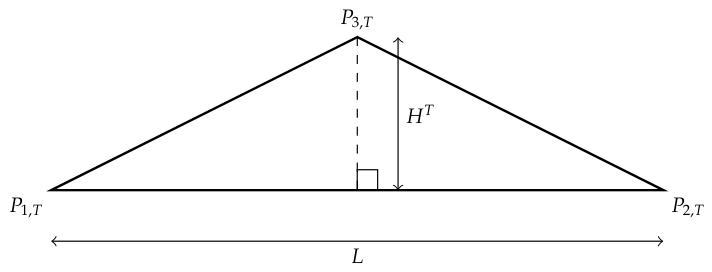
This LAISN option has two variants, namely, LAISN-3(1) and LAISN-3(2). Both variants assume that, in addition to the two transmitters located at either end of the leader, i.e., at $P_{1,T}$ and $P_{2,T}$, there is another transmitter halfway between $P_{1,T}$ and $P_{2,T}$. This transmitter, located at $P_{3,T}$, is, however, separated from the $P_{1,T}$–$P_{2,T}$ base by a distance $H^T$, forming an isosceles triangle with it—see Figure 1.

2.3.1. LAISN-3(1)

LAISN-3(1) is basically an option of LAISN-2 in which the position update is performed three times: first for the pair of transmitters $P_{1,T}$ and $P_{2,T}$, then for $P_{1,T}$ and $P_{3,T}$, and finally for $P_{2,T}$ and $P_{3,T}$. The three resulting position observations: ${\mathbf{z}}^{(p,1)}$, ${\mathbf{z}}^{(p,2)}$, and ${\mathbf{z}}^{(p,3)}$ are not statistically independent because the corresponding transmitter pairs share range measurements and common leader information. LAISN-3(1) deliberately neglects these correlations and performs three consecutive position updates without propagating the cross-covariances between the observations. Thus, this procedure should not be interpreted as a statistically consistent fusion of independent measurements, but as a simplified sequential-update strategy adopted within the proposed low-complexity navigation architecture. This approach can be written as follows:

$$({\widehat{\mathbf{x}}}_k^{-},{\mathbf{P}}_k^{-})\stackrel{{\mathrm{pos}}_1}{\to }({\widehat{\mathbf{x}}}_k^{(p,1)},{\mathbf{P}}_k^{(p,1)})\stackrel{{\mathrm{pos}}_2}{\to }({\widehat{\mathbf{x}}}_k^{(p,2)},{\mathbf{P}}_k^{(p,2)})\stackrel{{\mathrm{pos}}_3}{\to }({\widehat{\mathbf{x}}}_k^{(p,3)},{\mathbf{P}}_k^{(p,3)})$$

2.3.2. LAISN-3(2)

Unlike LAISN-3(1), LAISN-3(2) performs a single position update and works in several steps. First, the values $N^{\left(i\right)}$, $i=1,\dots ,3$ are calculated for each pair of transmitters. If $N^{\left(i\right)}=0$ for each pair, then LAISN-3(2) assumes that the follower’s position is exactly behind the leader by a distance $D_1$. i.e.,: ${\mathbf{z}}^{\left(p\right)}=P_{D_1}=movePoint(P_{1,T},D_1,reverseHeading\left({\theta }_L\right))$. Otherwise, LAISN-3(2) proceeds to the next step in which it calculates ${\mathbf{z}}^{\left(p\right)}$ and ${\sigma }_p$ for each pair of transmitters in a LAISN-2-like way:

$${\mathbf{z}}^{(p,i)}=\left\{\begin{array}{cc}{P}_{0,I}^{(k,l)}\hfill & N^{(k,l)}=1\hfill \\ P_{D_{(k,l)}}\hfill & N^{(k,l)}=2\mathrm{and}{D}^{P_{1,I},P_{2,I},(k,l)}<T\hfill \\ P_{1\left(2\right),I}^{(k,l)}\hfill & \mathrm{otherwise}\hfill \end{array}\right.,i=1,\dots ,3$$

(21)

$${\sigma }_{p,i}=\left\{\begin{array}{cc}0\hfill & N^{(k,l)}=1\mathrm{or}\hfill \\ \hfill & N^{(k,l)}=2\mathrm{and}{D}^{P_{1,I},P_{2,I},(k,l)}<T\hfill \\ \beta /D^{P_{1,I},P_{2,I},(k,l)}\hfill & \mathrm{otherwise}\hfill \end{array}\right.,i=1,\dots ,3$$

(22)

where

• $k,l=1,2$ for $i=1$, $k,l=1,3$ for $i=2$, and $k,l=2,3$ for $i=3$;
• $P_{0,I}^{(k,l)}$ is the single intersection point of circles k, l with centres at $P_{k,T}$ and $P_{l,T}$ and radii $D_k$ and $D_l$, respectively;
• $N^{(k,l)}$ is the number of intersection points of circles k, l;
• $P_{D_{(k,l)}}$ is the point behind the leader located on the line defined by points $P_{k,T}$, $P_{l,T}$:

  $$P_{D_{(k,l)}}=\left\{\begin{array}{cc}movePoint(P_{1,T},D_1,reverseHeading\left({\theta }_{P_{2,T}\to P_{1,T}}\right))\hfill & k,l=1,2\hfill \\ movePoint(P_{1,T},D_1,reverseHeading\left({\theta }_{P_{3,T}\to P_{1,T}}\right))\hfill & k,l=1,3\hfill \\ movePoint(P_{2,T},D_2,reverseHeading\left({\theta }_{P_{2,T}\to P_{3,T}}\right))\hfill & k,l=2,3\hfill \end{array}\right.$$
• $D^{P_{1,I},P_{2,I},(k,l)}=|\parallel (x^{-},y^{-})-P_{1,I}^{(k,l)}\parallel -\parallel (x^{-},y^{-})-P_{2,I}^{(k,l)}\parallel |$, and $P_{1,I}^{(k,l)}$, $P_{2,I}^{(k,l)}$ are two intersection point of circles k, l;
• $P_{1\left(2\right),I}^{(k,l)}=\arg {\min }_{P_i\in \{P_{1,I}^{(k,l)},P_{2,I}^{(k,l)}\}}\parallel P_i-(x^{-},y^{-})\parallel$.

The final step of LAISN-3(2) is to aggregate the three pairwise position estimates into a single position observation ${\mathbf{z}}^{\left(p\right)}$ and the associated confidence parameter ${\sigma }_p$:

$${\mathbf{z}}^{\left(p\right)}=(z_1^{\left(p\right)},z_2^{\left(p\right)})=\left(\xi ({\mathbf{Z}}_1^{\left(p\right)},{\Sigma }_p,\mathbf{N}),\xi ({\mathbf{Z}}_2^{\left(p\right)},{\Sigma }_p,\mathbf{N})\right)$$

(23)

$$\xi ({\mathbf{Z}}_k^{\left(p\right)},{\Sigma }_p,\mathbf{N})={\displaystyle \frac{{\sum }_{\begin{array}{c}i=1\\ N^{\left(i\right)}>0\end{array}}^3\frac{1}{1+{\sigma }_{p,i}}{z}_k^{(p,i)}}{{\sum }_{\begin{array}{c}i=1\\ N^{\left(i\right)}>0\end{array}}^3\frac{1}{1+{\sigma }_{p,i}}}}$$

(24)

$${\sigma }_p={\displaystyle \frac{1}{3}}{\displaystyle \sum _{i=1}^3}{\sigma }_{p,i}$$

(25)

where ${\Sigma }_p=\langle {\sigma }_{p,1},{\sigma }_{p,2},{\sigma }_{p,3}\rangle$, $\mathbf{N}=\langle N^{\left(1\right)},N^{\left(2\right)},N^{\left(3\right)}\rangle$, and ${\mathbf{Z}}_k^{\left(p\right)}=\langle z_k^{(p,1)},z_k^{(p,2)},z_k^{(p,3)}\rangle$, $k=1,2$, is the vector of k-th components of measurements ${\mathbf{z}}^{(p,i)}$.

It should be noted that the three pairwise position estimates used in the above aggregation are statistically correlated because they share range measurements and common leader information. The weighting rule in (24) and the calculation of ${\sigma }_p$ in (25) do not explicitly propagate the corresponding cross-covariances. Consequently, ${\sigma }_p$ should not be interpreted as a statistically derived standard deviation of the aggregated position estimate. Instead, it is an empirically defined confidence parameter used to control the weight assigned to the resulting position observation in the subsequent Kalman filter update. LAISN-3(2) therefore represents a simplified engineering fusion procedure rather than a statistically optimal fusion of correlated position estimates. This simplification was deliberately adopted to preserve the simple structure of the proposed navigation procedure, and its effectiveness was assessed empirically through the simulation experiments presented in this paper.

2.3.3. Other Possible LAISN-3 Variants

In addition to the two LAISN variants based on the three distance measurements specified above, two other variants were tested. However, because they proved very ineffective, they were not included in the paper.

The first omitted variant considers only one of the three available measurement baselines. This is the baseline with the highest measurement certainty. This certainty is estimated, as in LAISN-3(1) and LAISN-3(2), primarily by analysing parameter N and using distance $D^{P_{1,I},P_{2,I}}$. If $N=1$, then the given base is characterised by high certainty. If $N=2$, the certainty depends on the distance $D^{P_{1,I},P_{2,I}}$. The greater this distance, the greater the certainty. Of course, $N=0$ indicates very low certainty.

The second omitted variant is based primarily on the main baseline $P_{1,T}-P_{2,T}$. The remaining baselines are used only in two situations. The first is $N=0$ and the second is $D^{P_{1,I},P_{2,I}}<T$ for the main baseline.

2.4. Position Gross Errors

LAISN assumes the possibility of detecting gross errors in the estimated position, resulting mainly from acoustic signal reflections from the wavy sea surface. As mentioned above, LAISN assumes that the vehicle swarm moves close to the surface, which means other gross error sources, such as refraction, can be omitted with high probability.

Gross error detection involves estimating the distance the vehicle can travel at a given speed and whether the estimated position exceeds this distance. If this is the case, a gross error is present, and the position update step is rejected.

3. Experiments

3.1. Settings

To evaluate the effectiveness of the proposed system, a series of simulation-based experiments was conducted. The testing framework consisted of eight missions involving two vehicles: a leader and a follower. The leader, equipped with the system’s transmitting components (two/three acoustic transmitters), followed a predefined L-shaped trajectory on each mission, first moving east, then north, at a constant speed of 1 m/s. The total length of the leader’s path was 1000 m.

The initial position and velocity of both vehicles were assumed to be known accurately. This assumption reflects the intended operational scenario in which the vehicles start their mission at the surface, where their position and velocity can be determined using satellite navigation before submergence. These values are then used to initialise the navigation filter. Consequently, LAISN is intended to maintain the follower navigation solution after submergence rather than to determine an unknown initial position from acoustic range measurements alone. In the simulations, this surface-based initialisation was represented by setting the initial position and velocity uncertainties to zero.

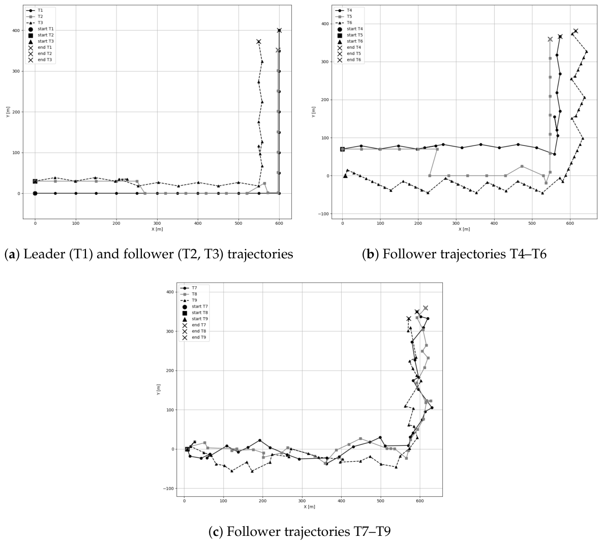
In contrast, the trajectory of the follower differed in each mission. These trajectories were generated randomly while satisfying a set of constraints, including the maximum allowable distance to the leader (50 or 100 m (a compact swarm is assumed in which the maximum distance between members does not exceed 100 m)), the distance between waypoints (shorter or longer), and the difference between the leader’s and follower’s headings (similar headings or drastic differences possible). Additionally, the follower operates with varying speeds across missions, with an upper limit of 3 m/s. All trajectories are depicted in Figure 2.

All simulations were conducted in the horizontal plane, i.e., without explicitly modelling the Z coordinate. The proposed system assumes that each follower knows both its own depth and the leader’s current depth. Consequently, the vertical separation between the two vehicles is known, and only the relative position in the horizontal $XY$ plane must be estimated. (One possible implementation assumes that the leader periodically transmits its current depth together with the acoustic messages, while both the leader and each follower measure their own depth using high-accuracy pressure sensors. Other mechanisms providing equivalent depth information may also be used and are outside the scope of this work).

Pressure sensors used in underwater vehicles provide highly accurate depth measurements and are not affected by the cumulative drift characteristic of dead-reckoning navigation systems. Consequently, the combined uncertainty in the leader and follower depths is expected to remain small compared with the horizontal localisation errors considered in this study.

Although the Z coordinate was not explicitly included in the geometric localisation model, the influence of small depth-related errors was not completely neglected. In the fourth stage of the simulation study, in which the influence of range-measurement errors was analysed, the imposed range errors were intentionally increased. This conservative assumption was introduced to account not only for the uncertainty of the acoustic ranging process itself, but also for small discrepancies between the actual and assumed depths of the leader and follower. Consequently, although the localisation algorithm was evaluated in a two-dimensional environment, the adopted range-error model implicitly accounted for the expected effects of realistic depth inaccuracies.

The vehicle motion was intentionally modelled using a simplified kinematic model, assuming a constant angular velocity of 10 deg/s during turning manoeuvres and a constant acceleration/deceleration of 0.2 m/s² during speed changes. These values were adopted as representative manoeuvring parameters and were kept constant throughout all validation scenarios. This simplification was intentional because the objective of this work was not to analyse vehicle dynamics or optimise motion parameters, but to evaluate the performance of the proposed low-cost leader–follower navigation architecture under a wide range of operating conditions. By using the same kinematic model in all simulations, the influence of vehicle dynamics was eliminated as an additional variable, allowing the localisation performance of the navigation architecture to be assessed in a consistent manner.

During each mission, the relative positions, relative bearings and relative velocities between the leader and the follower varied continuously. Acceleration and deceleration phases occurred whenever the vehicle speed changed, whereas constant-velocity motion was assumed after the desired speed had been reached. Consequently, the proposed low-cost leader–follower navigation system was evaluated over a broad range of relative motion conditions while avoiding unnecessary complexity associated with high-fidelity vehicle dynamics.

Since the relative localisation accuracy depends primarily on the geometry between the leader and the follower rather than on the detailed dynamic response of the vehicles, the adopted kinematic model was considered sufficient for evaluating the influence of the analysed system parameters on localisation performance.

The simulations also accounted for imperfections in navigation sensors. The leader was assumed to be equipped with a high-precision navigation system; therefore, its motion parameters in most simulation scenarios were treated as ground truth with no added noise. The exception was the scenario in which the influence of errors generated by the leader’s sensors was examined. In contrast, the follower’s measurements were always affected by noise, including errors in speed, heading, depth, and the distances to the transmitters mounted on the leader. The measurements performed by the vehicles and their errors were as follows:

$$v=\left|v_{\mathrm{true}}+\mathcal{N}({\mu }_v^S,{\sigma }_v^S)\right|$$

(26)

$$\theta ={\theta }_{true}+{\mu }_{\theta }^S+\left|\mathcal{N}({\mu }_{\theta }^S,{\sigma }_{\theta }^S)-{\mu }_{\theta }^S\right|$$

(27)

$$D_i=D_{i,\mathrm{true}}+{\tau }_i·\mathcal{U}(0,1)+{\displaystyle \frac{\psi ·D_{i,\mathrm{true}}}{{\max }_{j=1}^{N^T}{D}_j}}.$$

(28)

Equation (26), describing the measurement of the forward speed v, assumes that the speed remains strictly non-negative and that the measurement errors follow a Gaussian distribution. As a result, the measured value may be either lower or higher than the true speed, reflecting symmetric noise characteristics typical for such sensors.

A different situation is observed for the measurement of $\theta$, defined in Equation (27). In this case, the measured value is always greater than the true value and, moreover, exceeds ${\mu }_{\theta }^S$. This corresponds to a scenario in which inertial sensors exhibit a unidirectional drift. Consequently, the errors in $\theta$ are not Gaussian, in contrast to the assumptions commonly made in standard filtering approaches such as LAISN.

The range values $D_i$, $i=1,\dots ,N^T$ used by the localisation algorithm are modelled according to (28). The adopted error model represents the overall uncertainty affecting the range measurements, including the uncertainty of the acoustic ranging process itself, the cumulative effect of depth-measurement errors in both the leader and the follower, and residual time-synchronisation errors between the leader and follower clocks.

The model consists of two error components. The first component, controlled by ${\tau }_i$, is independent for each transmitter, allowing asymmetric range errors to be simulated. Such asymmetry may result, for example, from differences in acoustic propagation conditions affecting individual transmitters or from the vehicle geometry when the leader is not perfectly level, causing individual transmitters to be located at different depths relative to the point at which the leader depth is measured. The second component depends on the true distance and on the random variable $\psi \sim \mathcal{N}({\mu }_D^S,{\sigma }_D^S)$, which is common to all transmitters and represents the correlated part of the ranging error. Together, these two components enable both symmetric and asymmetric ranging-error scenarios to be reproduced, which can significantly affect the localisation accuracy of the proposed LAISN system.

In the experiments reported further, the parameters ${\tau }_i$, ${\mu }_D^S$, and ${\sigma }_D^S$ were not calibrated for any specific underwater environment. Instead, they were gradually increased over predefined ranges to represent progressively deteriorating ranging conditions. Consequently, lower parameter values correspond to higher-quality acoustic range measurements, whereas higher values represent increasing ranging uncertainty caused by any combination of environmental or system-related factors. This approach allows the robustness of the proposed navigation architecture to be evaluated independently of a particular acoustic propagation model or operating environment.

It should be noted that the adopted model does not explicitly simulate underwater acoustic propagation phenomena such as multipath propagation, sound-speed stratification or ray bending. As discussed in the Introduction, the proposed LAISN system is intended for swarms operating at relatively short inter-vehicle distances and similar depths, where the direct propagation path is expected to dominate. Consequently, these effects are represented implicitly through the adopted stochastic ranging-error model rather than by modelling the acoustic propagation process itself.

Numerical values of all simulation parameters are as follows: simulation and LAISN step $\Delta t$ = 0.1 s, distance measurement timestep $\Delta t_D$ = 1, 5 or 10 s, $\alpha =8$, ${\sigma }_a^0=60$, $p_{po{s}_{s}td}=0$, $p_{ve{l}_{s}td}=0$, T = 0.1 or 10, $\beta$ = 0.1 or 100, ${\mu }_v=v$, ${\sigma }_v={\sigma }_v^S$ = 0.2 m/s, ${\mu }_{\theta }=\theta$, ${\sigma }_{\theta }={\sigma }_{\theta }^S=2$ deg, ${\mu }_v^S=0.2$ m/s, ${\mu }_{\theta }^{S,\mathrm{follower}}=5$ deg, ${\mu }_{\theta }^{S,\mathrm{leader}}$= 0, 2.5, or 5 deg, $\tau$ = 0.01, 0.03 or 0.06 m, ${\mu }_D^S$ = 0.1 or 0.3 m, ${\sigma }_D^S$ = 0.01 or 0.05 m, the distance of the third leader’s transmiter to the base $P_{1,T}-P_{2,T}$$H^T$ = 0.1 or 0.2 m, the length of the leader L = 1 or 2 m.

All parameters crucial for LAISN performance, such as $\alpha$, ${\sigma }_a^0$, T, and $\beta$, were selected manually without any optimisation process. Regarding vehicle speed measurement errors, the values ${\mu }_v^S=0.2$ m/s and ${\sigma }_v^S=0.2$ m/s were determined based on experience with electromagnetic speed logs and are considered highly probable errors. Even larger errors occurred during tests with a real vehicle equipped with such a log, but these were exceptional situations. Heading errors—${\mu }_{\theta }^{S,\mathrm{follower}}=5$ deg, ${\sigma }_{\theta }^S=2$ deg — correspond to a situation in which the combined use of accelerometers and magnetometers keeps the error in check, preventing it from growing significantly beyond 5 degrees. As before, this limit results from experience with good-quality, inexpensive inertial sensors. In the case of distance errors, the values ${\mu }_D^S$ = 0.1 or 0.3 m, ${\sigma }_D^S=0.01$ or 0.05 m result from preliminary tests of the proposed system in a swimming pool using Aquarian Audio hydrophones model AS-1 as a transmitting transducer and model S1n as a receiving transducer, and obtaining an average measurement error of 43.4 mm. The adopted error values are intentionally higher than those obtained for the laboratory system to assess the quality of the LAISN under less favourable acoustic signal propagation conditions and at larger distances between the leader and the follower.

3.2. Results

The study was divided into five stages, in which the influence of the following factors on the accuracy of the LAISN was examined: follower trajectory (T2–T9)—Stage 1; the distance-measurement timestep $\Delta t_D$—Stage 2; arrangement of leader’s transmitters (L, $H^T$)—Stage 3; distance errors ($\tau$, ${\mu }_D^S$, ${\sigma }_D^S$)—Stage 4; leader’s heading errors (${\mu }_{\theta }^{S,\mathrm{leader}}$)—Stage 5. To evaluate the LAISN at each stage, the system was run 60 times for each trajectory and set of parameters to account for the influence of randomness on measurement errors. The LAISN evaluation involved determining the maximum and mean errors for the estimated position $E^P=\parallel (x_{true},y_{true})-(\widehat{x},\widehat{y})\parallel$ and relative bearing $E^B=angleDiff(B_{true},\widehat{B})$, from all 60 runs, where $angleDiff$ is the difference between two angles.

3.2.1. Stage 1

This stage was run with the following parameters: $L=2$ m, $\Delta t$ = 0.1 s, $\Delta t_D$ = 1 s, $\tau$ = 0.01, ${\mu }_D^S$ = 0.1$,{\sigma }_D^S$ = 0.05 and its results are given in

Table 1. Results of Stage 1.

	${\mathit{E}}_{\mathit{max}}^{\mathit{P}}$[m]	${\mathit{E}}_{\mathit{max}}^{\mathit{B}}$[deg]	${\mathit{E}}_{\mathit{mean}}^{\mathit{P}}$[m]	${\mathit{E}}_{\mathit{mean}}^{\mathit{S}}$[deg]	${\mathit{\sigma }}^{\mathit{P}}$[m]	${\mathit{\sigma }}^{\mathit{B}}$[deg]
T2 LAISN-2	5.12	6.38	1.24	1.26	1.35	1.41
T2 LAISN-3(1)	7.54	10.55	1.35	1.42	1.51	1.62
T2 LAISN-3(2)	5.11	6.82	1.26	1.28	1.47	1.49
T3 LAISN-2	1.93	1.8	0.32	0.27	0.31	0.29
T3 LAISN-3(1)	2.79	2.50	0.44	0.39	0.44	0.40
T3 LAISN-3(2)	2.05	1.91	0.32	0.27	0.32	0.29
T4 LAISN-2	1.83	1.54	0.37	0.23	0.33	0.21
T4 LAISN-3(1)	2.17	1.87	0.40	0.26	0.35	0.27
T4 LAISN-3(2)	1.88	1.58	0.38	0.24	0.32	0.23
T5 LAISN-2	6.95	4.85	0.37	0.24	0.56	0.41
T5 LAISN-3(1)	12.81	8.70	0.53	0.36	1.23	0.86
T5 LAISN-3(2)	6.49	4.54	0.37	0.24	0.57	0.41
T6 LAISN-2	4.09	10.84	0.29	0.48	0.38	0.89
T6 LAISN-3(1)	5.69	27.35	0.50	0.98	0.68	1.92
T6 LAISN-3(2)	4.11	11.54	0.29	0.48	0.36	0.94
T7 LAISN-2	6.78	8.44	0.65	0.81	0.84	1.02
T7 LAISN-3(1)	11.60	16.57	1.53	1.92	1.94	2.53
T7 LAISN-3(2)	8.10	10.36	0.67	0.84	0.86	1.16
T8 LAISN-2	6.02	28.14	0.8	1.19	0.93	2.24
T8 LAISN-3(1)	9.55	28.71	1.52	2.16	1.77	2.78
T8 LAISN-3(2)	6.12	60.06	0.81	1.26	0.92	2.18
T9 LAISN-2	7.49	16.77	0.75	0.61	0.78	0.91
T9 LAISN-3(1)	12.43	29.00	1.18	1.01	1.77	2.03
T9 LAISN-3(2)	7.39	15.26	0.75	0.61	0.76	0.88

, and Figure 3.

Regarding the test trajectories, the table shows that T3 and T4 are the easiest for LAISN. These trajectories contain few turns, and, what is more, the turns are very gentle. Another important feature of these trajectories is that the follower is never directly behind the leader, meaning there is no situation where $B=180$ deg.

The table also shows that adding a third transmitter on the leader did not improve the results; this is the situation we are addressing in LAISN-3(2). In LAISN-3(1), it even worsened the results. The result obtained by LAISN-3(1) may be due to the fact that this variant of LAISN treats all measurements equally, even though the base length in the case of pairs $P_{1,T}$–$P_{3,T}$ and $P_{2,T}$–$P_{3,T}$ is smaller than in the case of the basic pair $P_{1,T}$–$P_{2,T}$, which affects the measurement accuracy.

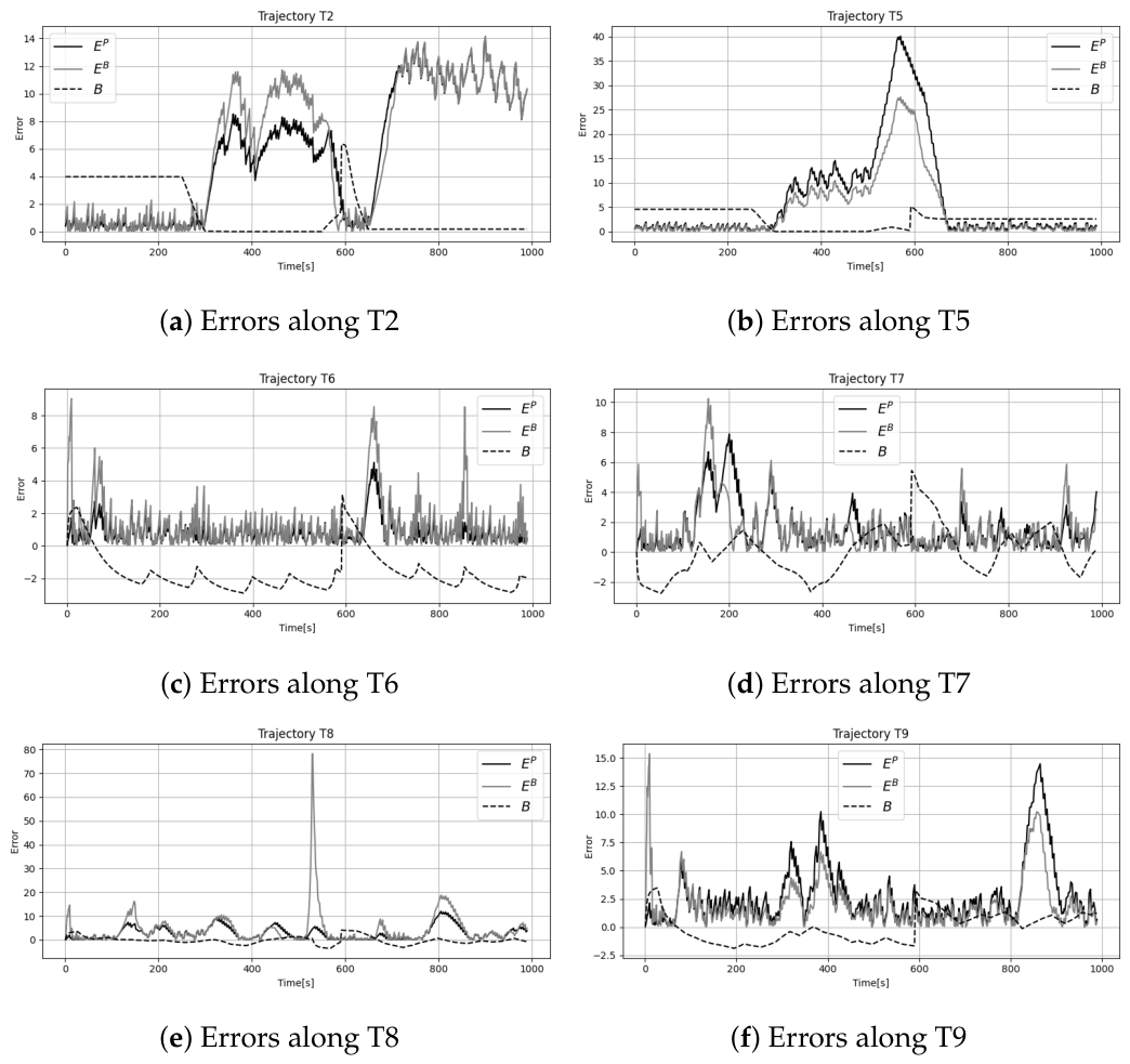
A more detailed analysis of the LAISN-2 results, that is, the best variant in Stage 1, for all the trajectories except T3 and T4, is given in Figure 3. The graphs in the figure, in addition to the $E^P$ and $E^B$ errors, also include the actual B, scaled to the <−10, 10> range. This means that B = 10 in the graphs is actually B = 360 deg, B = 0 in the graphs is actually B = 180 deg, and B = −10 in the graph is actually B = 0 deg. This procedure was necessary so that B could be presented together with errors that fall within narrower ranges than B.

All of the graphs show that the largest errors occur for B close to 180 deg. Four different situations are then possible:

• $N=1$, which is the ideal situation, and it is unlikely to be a reason for the errors—there is one point of intersection of the circles exactly behind the leader, so there is no doubt about the position of the follower;
• $N=2$, where one intersection point is selected as the follower location, but this selection is characterised by a high uncertainty resulting from the small distance between both points $D^{P_{1,I},P_{2,I}}$—high measurement uncertainty causes LAISN to focus more on the prediction and speed/heading measurements which are also subject to a high error;
• $N=2$, ${\sigma }_p=0$ and very small $D^{P_{1,I},P_{2,I}}$ which moves follower position centrally behind the leader—even though there are two potential points where the follower can be located, these points are so close to each other that it is difficult to choose the right one and LAISN assumes that it is one point, i.e., $N=1$, selecting only one of these points in this situation, i.e., the one closer to the estimated position $(x^{-},y^{-})$, often led to even larger errors;
• $N=0$, which, like in the previous case, forces the follower position to be adjusted to a position centrally behind the leader, accepting the possible error.

Despite the errors, the obtained results, with the exception of T8 and LAISN-3(1), appear satisfactory, especially since the largest errors appear quickly and quickly disappear to small values close to the mean errors.

In the case of T8, there is one point on the trajectory for which the $E^P$ error is still small, but the $E^B$ error increases to alarmingly large values—see Figure 3e. This occurs at the same point for all 60 runs. In this case, the follower speed is the culprit. This speed, which is approximately 1 m/s for most of the trajectory, briefly increases to 3 m/s at the point of the largest $E^B$ error. Combining this momentary acceleration with a follower heading error greater than ${\mu }_{\theta }^S=5$ deg, results in a rapid increase in the $E^B$ error. However, this increase is temporary and lasts about 30 s.

3.2.2. Stage 2

This stage was performed for three parameter settings: (i) $\Delta t=0.1$ s, $\Delta t_D=5$ s, (ii) $\Delta t=0.1$ s, $\Delta t_D=10$ s, and (iii) $\Delta t=1$ s, $\Delta t_D=10$ s. The parameter $\Delta t$ denotes the execution interval of the localisation algorithm, during which the follower updates its state estimate using the available onboard navigation sensors and, whenever available, the latest acoustic range measurements. The parameter $\Delta t_D$ denotes the effective interval between consecutive acoustic localisation updates. Although this interval may result from a reduced transmission rate selected by the leader, it may also represent packet losses, missed signal detections or other communication-related effects that prevent the follower from receiving consecutive acoustic measurements. Consequently, the adopted values of $\Delta t_D$ should be interpreted as the effective localisation update interval rather than the physical transmission interval of the acoustic messages. From the perspective of the localisation algorithm, these situations are equivalent because, in all cases, the state estimate is propagated using only the onboard navigation sensors until the next valid acoustic measurement becomes available.

In this stage $\Delta t_D$ was limited to the range from 1 s to 10 s. The lower bound of 1 s was not imposed by the proposed localisation algorithm but reflects practical considerations associated with underwater acoustic communication, including communication load and energy consumption. Since the objective of this work was to investigate the influence of update frequency on navigation performance rather than communication system design, shorter update intervals were not considered. The upper bound of 10 s was selected to investigate the practical operating limit of the proposed navigation architecture under increasingly infrequent navigation updates. As demonstrated in the simulation results, update intervals of approximately 10 s represent the upper limit for reliable operation, particularly during manoeuvring conditions, whereas shorter intervals are required to maintain formation stability.

Apart from the values of $\Delta t$ and $\Delta t_D$, all remaining simulation parameters were identical to those used in the previous stage.

The results of this stage are presented in

Table 2. Maximum errors in Stage 2.

	$\mathbf{\Delta }\mathit{t}$ = 0.1 s, $\mathbf{\Delta }{\mathit{t}}_{\mathit{D}}$ = 5 s		$\mathbf{\Delta }\mathit{t}$ = 0.1 s, $\mathbf{\Delta }{\mathit{t}}_{\mathit{D}}$ = 10 s		$\mathbf{\Delta }\mathit{t}$ = 1 s, $\mathbf{\Delta }{\mathit{t}}_{\mathit{D}}$ = 10 s
	${\mathit{E}}_{\mathit{max}}^{\mathit{P}}$[m]	${\mathit{E}}_{\mathit{max}}^{\mathit{B}}$[deg]	${\mathit{E}}_{\mathit{max}}^{\mathit{P}}$[m]	${\mathit{E}}_{\mathit{max}}^{\mathit{B}}$[deg]	${\mathit{E}}_{\mathit{max}}^{\mathit{P}}$[m]	${\mathit{E}}_{\mathit{max}}^{\mathit{B}}$[deg]
T2 LAISN-2	13.6	12.02	31.13	31.07	12.16	17.0
T2 LAISN-3(2)	14.00	12.54	29.61	29.13	70.17	81.20
T3 LAISN-2	2.12	1.96	9.91	7.72	7.26	5.26
T3 LAISN-3(2)	2.16	2.13	9.41	7.79	92.16	108.54
T4 LAISN-2	1.97	2.24	9.12	8.69	4.24	5.14
T4 LAISN-3(2)	1.95	2.12	8.68	8.65	47.60	38.55
T5 LAISN-2	5.36	3.77	19.63	14.88	15.05	10.79
T5 LAISN-3(2)	6.26	3.61	24.98	19.23	109.81	71.83
T6 LAISN-2	4.15	11.0	35.32	85.55	17.29	46.26
T6 LAISN-3(2)	4.69	12.14	34.03	85.87	62.79	138.03
T7 LAISN-2	8.36	10.29	40.29	77.27	40.3	71.84
T7 LAISN-3(2)	9.58	12.56	40.95	77.45	43.92	85.43
T8 LAISN-2	7.82	87.78	22.99	140.63	25.16	104.56
T8 LAISN-3(2)	8.19	91.00	23.07	144.15	56.90	179.99
T9 LAISN-2	5.83	16.52	10.82	18.45	24.64	23.68
T9 LAISN-3(2)	5.79	17.12	14.74	17.46	63.37	76.82

,

Table 3. Mean errors in Stage 2.

	$\mathbf{\Delta }\mathit{t}$ = 0.1 s, $\mathbf{\Delta }{\mathit{t}}_{\mathit{D}}$ = 5 s		$\mathbf{\Delta }\mathit{t}$ = 0.1 s, $\mathbf{\Delta }{\mathit{t}}_{\mathit{D}}$ = 10 s		$\mathbf{\Delta }\mathit{t}$ = 1 s, $\mathbf{\Delta }{\mathit{t}}_{\mathit{D}}$ = 10 s
	${\mathit{E}}_{\mathit{mean}}^{\mathit{P}}$[m]	${\mathit{E}}_{\mathit{mean}}^{\mathit{B}}$[deg]	${\mathit{E}}_{\mathit{mean}}^{\mathit{P}}$[m]	${\mathit{E}}_{\mathit{mean}}^{\mathit{B}}$[deg]	${\mathit{E}}_{\mathit{mean}}^{\mathit{P}}$[m]	${\mathit{E}}_{\mathit{mean}}^{\mathit{B}}$[deg]
T2 LAISN-2	2.04	1.93	9.65	9.02	3.04	3.29
T2 LAISN-3(2)	2.19	2.04	9.45	8.87	18.29	19.92
T3 LAISN-2	0.47	0.33	2.96	1.6	1.65	1.15
T3 LAISN-3(2)	0.48	0.34	3.05	1.62	29.27	25.31
T4 LAISN-2	0.48	0.25	2.9	1.18	1.06	0.57
T4 LAISN-3(2)	0.48	0.26	2.95	1.17	21.02	10.36
T5 LAISN-2	0.55	0.27	5.62	2.16	1.95	1.04
T5 LAISN-3(2)	0.57	0.28	6.13	2.36	23.19	9.18
T6 LAISN-2	0.52	0.89	16.36	23.8	3.02	5.47
T6 LAISN-3(2)	0.53	0.91	16.62	24.21	25.46	35.44
T7 LAISN-2	0.98	1.06	14.2	16.36	6.04	7.47
T7 LAISN-3(2)	1.04	1.09	15.51	18.22	15.99	21.46
T8 LAISN-2	1.1	1.96	8.19	12.21	6.2	8.61
T8 LAISN-3(2)	1.17	2.05	8.35	12.58	17.51	26.40
T9 LAISN-2	0.77	0.63	4.16	2.64	3.22	2.47
T9 LAISN-3(2)	0.78	0.64	4.64	2.87	24.90	18.28

and

Table 4. Standard deviations in Stage 2.

	$\mathbf{\Delta }\mathit{t}$ = 0.1 s, $\mathbf{\Delta }{\mathit{t}}_{\mathit{D}}$ = 5 s		$\mathbf{\Delta }\mathit{t}$ = 0.1 s, $\mathbf{\Delta }{\mathit{t}}_{\mathit{D}}$ = 10 s		$\mathbf{\Delta }\mathit{t}$ = 1 s, $\mathbf{\Delta }{\mathit{t}}_{\mathit{D}}$ = 10 s
	${\sigma }_{{\mathit{E}}^{\mathit{P}}}$[m]	${\sigma }_{{\mathit{E}}^{\mathit{B}}}$[deg]	${\sigma }_{{\mathit{E}}^{\mathit{P}}}$[m]	${\sigma }_{{\mathit{E}}^{\mathit{B}}}$[deg]	${\sigma }_{{\mathit{E}}^{\mathit{P}}}$[m]	${\sigma }_{{\mathit{E}}^{\mathit{B}}}$[deg]
T2 LAISN-2	2.14	2.22	6.21	6.01	3.52	3.62
T2 LAISN-3(2)	2.43	2.19	6.36	5.75	14.39	21.39
T3 LAISN-2	0.26	0.31	1.48	1.46	0.85	0.76
T3 LAISN-3(2)	0.29	0.28	1.56	1.41	17.70	18.10
T4 LAISN-2	0.22	0.19	1.58	1.56	0.64	0.35
T4 LAISN-3(2)	0.27	0.23	1.55	1.51	9.43	9.96
T5 LAISN-2	0.51	0.27	3.72	2.19	1.42	0.98
T5 LAISN-3(2)	0.49	0.31	3.81	2.24	21.66	10.54
T6 LAISN-2	0.45	1.32	7.99	15.41	3.33	4.52
T6 LAISN-3(2)	0.49	1.28	8.08	15.29	13.82	16.20
T7 LAISN-2	1.01	1.47	9.15	16.99	5.28	6.87
T7 LAISN-3(2)	1.10	1.42	9.22	17.21	10.01	15.38
T8 LAISN-2	0.95	4.56	4.19	15.89	6.94	8.25
T8 LAISN-3(2)	1.03	4.74	4.28	16.02	11.60	29.40
T9 LAISN-2	0.61	1.05	1.145	1.81	2.03	1.84
T9 LAISN-3(2)	0.65	1.19	1.85	1.83	15.39	11.98

and include the performance of the two most effective LAISN variants in the previous stage, i.e., LAISN-2 and LAISN-3(2). They reveal that increasing $\Delta t_D$ to 5 s does not significantly affect the deterioration in estimate accuracy. The problem only appears at $\Delta t_D$ = 10 s. In this case, position and bearing errors increase to unacceptable levels for an in-swarm localisation system, with position errors reaching 30–40 m and relative bearing errors reaching 30–140 deg. The exceptions are T2, T3, T4, and T5 trajectories, which are stable in heading and follower speed, and the scenario with $\Delta t$ = 1 s and the LAISN-2 application. In this case, both the maximum and mean errors are noticeably smaller than in the other cases.

The tables also confirm what was achieved in Stage 1: no noticeable improvement in LAISN performance after adding an additional leader’s transmitter. For most of the cases studied, the accuracy of LAISN-2 and LAISN-3(2) is similar, but the difference appears for $\Delta t$ = 1 s and $\Delta t_D$ = 10 s. In this case, the advantage of LAISN-2 over LAISN-3(2) is undeniable.

The detailed results of LAISN-2 are also given in Figure 4 and Figure 5. They reveal that if B = 0 (180 deg) over most of the trajectory (trajectory T2), then frequent position updates are necessary, as was the case in Stage 1. Otherwise, as shown in Figure 4a, even a position update interval of $\Delta t_D$ = 5 s ultimately results in a rapid increase in error. In this figure, the error over 1 km is 14 m, but it will continue to grow rapidly. In the remaining cases, although the error is larger than for $\Delta t_D$ = 1 s and spikes are still visible near B = 0 (180 deg), there is no situation in which the error begins to grow rapidly and uncontrollably.

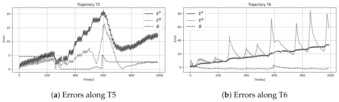
Increasing $\Delta t_D$ to 10 s, and leaving $\Delta t$ at 0.1 s, except for trajectories T3 and T4, which remain consistently away from B = 0 (180 deg), results in a gradual, successive increase in error. This error is not very large over 1km because the largest error $E^P$ in this setting, as shown in Table 2, occurs for T7 and amounts to 40 m. However, there is a visible trend towards an increase in this error, as shown in Figure 5 for trajectories T5 and T6. The same situation occurs for the remaining trajectories, excluding the previously mentioned T3 and T4.

As mentioned above, the situation can be improved by increasing $\Delta t$ to 1 s—see Figure 6. However, this improvement applies only to the previously mentioned trajectories T2, T3, T4, and T5, in which the follower does not perform major manoeuvres and maintains a stable speed.

3.2.3. Stage 3

This stage was run for two different settings: $L=1$ m, $H^T=0.1$ m, and $L=2$ m, $H^T=0.2$ m. In both cases, $\Delta t_D=5$ s. The remaining parameters were the same as in Stage 1.

The results for $L=1$ m are presented in

Table 5. Results in Stage 3 for $L=1$ m, $H^T=0.1$ m.

	${\mathit{E}}_{\mathit{max}}^{\mathit{P}}$[m]	${\mathit{E}}_{\mathit{max}}^{\mathit{B}}$[deg]	${\mathit{E}}_{\mathit{mean}}^{\mathit{P}}$[m]	${\mathit{E}}_{\mathit{mean}}^{\mathit{S}}$[deg]	${\mathit{\sigma }}^{\mathit{P}}$[m]	${\mathit{\sigma }}^{\mathit{B}}$[deg]
T2 LAISN-2	12.52	11.09	2.22	2.11	2.01	1.98
T2 LAISN-3(2)	13.42	11.97	1.94	1.88	2.29	2.12
T3 LAISN-2	2.61	2.32	0.56	0.43	0.38	0.39
T3 LAISN-3(2)	2.82	2.60	0.58	0.45	0.37	0.37
T4 LAISN-2	2.57	2.38	0.59	0.35	0.33	0.27
T4 LAISN-3(2)	2.40	2.23	0.60	0.35	0.34	0.29
T5 LAISN-2	8.2	5.83	0.76	0.41	0.71	0.46
T5 LAISN-3(2)	6.41	4.53	0.71	0.39	0.66	0.43
T6 LAISN-2	4.84	12.49	0.56	0.96	0.54	1.35
T6 LAISN-3(2)	5.50	11.94	0.60	1.04	0.59	1.44
T7 LAISN-2	8.55	10.78	1.08	1.14	1.15	1.45
T7 LAISN-3(2)	9.34	11.64	1.24	1.29	1.28	1.56
T8 LAISN-2	8.43	88.97	1.27	2.1	1.16	4.44
T8 LAISN-3(2)	9.09	86.41	1.36	2.27	1.14	4.48
T9 LAISN-2	7.52	15.8	0.98	0.78	0.83	1.25
T9 LAISN-3(2)	7.24	16.30	1.00	0.79	0.88	1.27

and show that, compared to a previous system configuration, shortening the system base to 1m degrades performance only slightly.

Moving $P_{3,T}$ farther from the base to $H^T=0.2$ m, with the leader length again set to 2 m, had practically no effect on system accuracy—see

Table 6. Results in Stage 3 for $L=2$ m, $H^T=0.2$ m.

	${\mathit{E}}_{\mathit{max}}^{\mathit{P}}$[m]	${\mathit{E}}_{\mathit{max}}^{\mathit{B}}$[deg]	${\mathit{E}}_{\mathit{mean}}^{\mathit{P}}$[m]	${\mathit{E}}_{\mathit{mean}}^{\mathit{S}}$[deg]	${\mathit{\sigma }}^{\mathit{P}}$[m]	${\mathit{\sigma }}^{\mathit{B}}$[deg]
T2 LAISN-3(2)	14.34	13.35	1.95	1.85	2.43	2.21
T3 LAISN-3(2)	2.36	2.20	0.48	0.34	0.30	0.29
T4 LAISN-3(2)	1.92	2.34	0.49	0.26	0.28	0.24
T5 LAISN-3(2)	5.78	3.70	0.56	0.28	0.51	0.32
T6 LAISN-3(2)	5.11	12.27	0.56	0.98	0.55	1.40
T7 LAISN-3(2)	9.18	11.77	1.07	1.10	1.11	1.41
T8 LAISN-3(2)	6.92	89.65	1.24	2.27	1.08	5.05
T9 LAISN-3(2)	6.59	17.19	0.83	0.68	0.72	1.25

. The changes compared to the $H^T=0.1$ m version are almost imperceptible.

Research into further extensions of $H^T$ to values of 0.3, 0.4 m, etc., was discontinued due to the impracticality of such solutions. $H^T=0.3$ or 0.4 m would have required extending the transmitter beyond the leader’s hull, which would have drastically increased drag and, consequently, leader performance.

3.2.4. Stage 4

At this stage, the leader length returned to L = 2 m, and $\Delta t_D$ remained at 5 s. In this case, the parameters responsible for the distance-measurement error were modified. First, a scenario was analysed in which the distance-measurement error for all transmitters was increased with respect to Stage 1 while remaining identical for each transmitter. To achieve this, ${\mu }_D^S$ and ${\sigma }_D^S$ were increased to 0.3 m and 0.05 m, respectively.

The adopted error values were intentionally selected to represent not only the uncertainty of the acoustic ranging process itself, but also the cumulative influence of small depth-estimation errors of both the leader and the follower. Although LAISN assumes that the current depths of both vehicles are available, these values are still affected by finite measurement accuracy. Consequently, the increased ranging error used in this stage should be interpreted as a conservative equivalent error that combines the acoustic ranging uncertainty with the expected influence of realistic depth inaccuracies.

Assuming that the maximum distance between the leader and the follower is 100 m, and considerably smaller during most of the mission, while the swarm operates at relatively shallow depths where the influence of sound-speed stratification is limited, a distance-measurement error of 0.3 m can be considered relatively large, although still realistic based on the authors’ experience with underwater acoustic measurements.

Despite the increase in distance measurement errors associated with each transmitter to levels that should have caused a noticeable degradation in system accuracy, the effect was barely noticeable, with only a slight increase in mean errors.

In the next step, the previous ${\mu }_D^S$ and ${\sigma }_D^S$ values were restored, while $\tau$ was increased first to 0.03 and then to 0.06. As a result, the measurement errors associated with different transmitters became increasingly asymmetric. Such asymmetry may arise for at least two reasons. First, although relatively unlikely, individual acoustic signals may propagate along slightly different paths due to local environmental conditions, resulting in different ranging errors for different transmitters. Second, when the leader is not perfectly level—i.e., its pitch angle differs from zero—individual transmitters may be located at different depths relative to the point at which the leader depth is measured. Consequently, although all range measurements are affected by the acoustic ranging error, the depth-related error component may differ for individual transmitters. Therefore, different transmitters may exhibit different effective ranging errors.

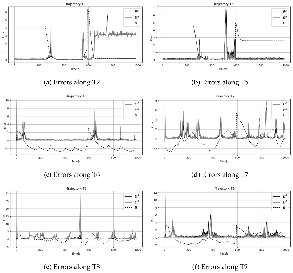
As expected, increasing $\tau$ degraded the localisation accuracy, although the deterioration remained relatively small. A more pronounced effect was observed only when $\tau =0.06$ was assigned to one transmitter and $\tau =0.01$ to the remaining transmitters, corresponding to a strongly asymmetric distribution of effective ranging errors.

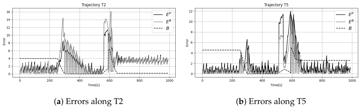
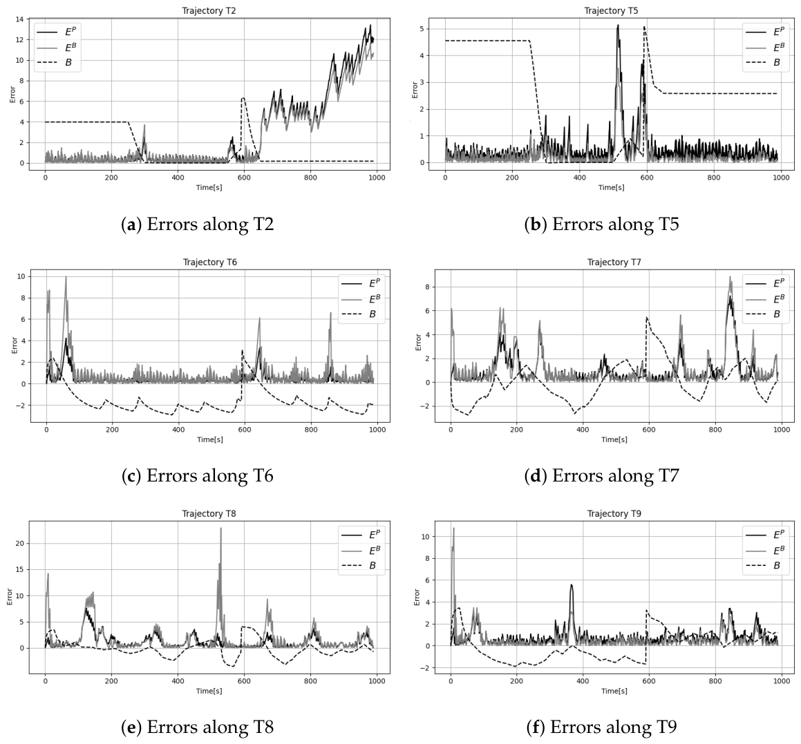
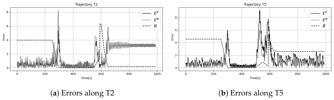
The results for this setting are presented in

Table 7. Results in Stage 4.

	${\mathit{E}}_{\mathit{max}}^{\mathit{P}}$[m]	${\mathit{E}}_{\mathit{max}}^{\mathit{B}}$[deg]	${\mathit{E}}_{\mathit{mean}}^{\mathit{P}}$[m]	${\mathit{E}}_{\mathit{mean}}^{\mathit{S}}$[deg]	${\mathit{\sigma }}^{\mathit{P}}$[m]	${\mathit{\sigma }}^{\mathit{B}}$[deg]
T2 LAISN-2	14.23	14.38	4.35	4.68	4.5	4.75
T2 LAISN-3(2)	6.80	9.43	1.58	1.67	1.38	1.46
T3 LAISN-2	3.59	3.20	0.9	0.8	0.58	0.57
T3 LAISN-3(2)	6.51	5.86	1.26	1.12	1.11	1.00
T4 LAISN-2	3.68	3.27	1.06	0.69	0.62	0.48
T4 LAISN-3(2)	4.47	3.77	1.17	0.78	0.83	0.64
T5 LAISN-2	40.08	27.54	5.16	3.49	9.86	6.63
T5 LAISN-3(2)	12.61	8.96	1.32	0.90	1.61	1.15
T6 LAISN-2	5.16	13.30	0.83	1.42	0.82	1.86
T6 LAISN-3(2)	6.78	12.87	0.77	1.30	0.60	1.45
T7 LAISN-2	9.10	14.58	1.52	1.65	1.72	2.37
T7 LAISN-3(2)	14.36	20.72	2.08	2.48	1.96	2.45
T8 LAISN-2	11.59	91.35	2.30	3.70	2.38	6.40
T8 LAISN-3(2)	10.01	85.75	2.05	3.23	1.65	4.82
T9 LAISN-2	14.22	16.40	2.12	1.58	2.52	1.99
T9 LAISN-3(2)	15.38	16.79	2.71	2.09	2.47	2.06

and Figure 7 and Figure 8, which show a general deterioration in performance for each trajectory regardless of LAISN variant. However, the most interesting effect was observed for trajectories T2 and T5, which are characterised by long sections in which the follower moves exactly behind the leader ($B=180$ deg). It turned out that these trajectories, due to large asymmetries in distance measurements, pose a significant problem for LAISN-2 (see Figure 7a,b). At the same time, LAISN-3(2) achieves significantly better results for the same trajectories (see Figure 8).

The advantage of LAISN-3(2) over LAISN-2 for large asymmetries in distance measurement errors most likely stems from the fact that LAISN-3(2), unlike LAISN-2, has three sources of position information, i.e., baselines: $P_{1,T}$–$P_{2,T}$, $P_{1,T}$–$P_{3,T}$, and $P_{2,T}$–$P_{3,T}$. The distance measurement to $P_{1,T}$, due to $\tau =0.06$, is significantly less accurate than for $P_{2,T}$ and $P_{3,T}$, for which $\tau =0.01$. This makes the position measurement based on $P_{1,T}$, i.e., baselines $P_{1,T}$–$P_{2,T}$, and $P_{1,T}$–$P_{3,T}$, significantly less accurate than the measurement based on the less noisy baseline $P_{2,T}$–$P_{3,T}$. LAISN-2 relies on only one strongly noisy baseline $P_{1,T}$–$P_{2,T}$, which generates a large error. In contrast, LAISN-3(2) uses all three baselines, including one that is the least disturbed.

3.2.5. Stage 5

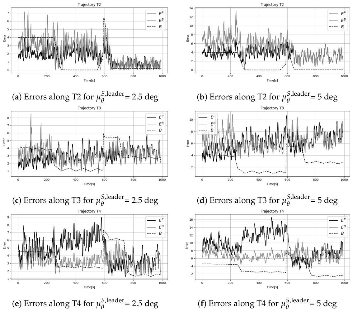
The aim of this stage was to investigate the sensitivity of the LAISN to leader heading errors, which cause all measurement baselines $P_{1,T}$–$P_{2,T}$, $P_{1,T}$–$P_{3,T}$, and $P_{2,T}$–$P_{3,T}$ to rotate by an error angle. The leader heading error was generated according to (27) with ${\mu }_{\theta }^{S,\mathrm{leader}}$ = 2.5 or 5 deg. The remaining parameters were the same as in Stage 1. Results of this stage are given in

Table 8. Results in Stage 5 for ${\mu }_{\theta }^{S,\mathrm{leader}}$= 2.5 deg.

	${\mathit{E}}_{\mathit{max}}^{\mathit{P}}$[m]	${\mathit{E}}_{\mathit{max}}^{\mathit{B}}$[deg]	${\mathit{E}}_{\mathit{mean}}^{\mathit{P}}$[m]	${\mathit{E}}_{\mathit{mean}}^{\mathit{S}}$[deg]	${\mathit{\sigma }}^{\mathit{P}}$[m]	${\mathit{\sigma }}^{\mathit{B}}$[deg]
T2 LAISN-2	4.67	8.30	1.57	2.20	0.81	1.49
T2 LAISN-3(2)	4.83	8.68	1.58	2.20	0.83	1.50
T3 LAISN-2	6.73	8.69	2.89	3.06	0.95	0.99
T3 LAISN-3(2)	6.63	8.70	2.90	3.07	0.96	1.01
T4 LAISN-2	10.44	8.22	4.57	3.25	1.73	0.86
T4 LAISN-3(2)	10.84	8.87	4.59	3.26	1.71	0.86
T5 LAISN-2	9.12	7.40	4.00	3.06	1.25	1.12
T5 LAISN-3(2)	8.06	6.54	4.00	3.05	1.21	1.00
T6 LAISN-2	5.50	12.91	2.19	3.30	0.95	1.34
T6 LAISN-3(2)	5.92	13.12	2.21	3.33	0.98	1.37
T7 LAISN-2	9.37	11.21	2.34	2.92	1.28	1.65
T7 LAISN-3(2)	8.77	10.74	2.36	2.91	1.29	1.63
T8 LAISN-2	9.88	53.37	2.54	3.52	1.64	2.35
T8 LAISN-3(2)	10.06	65.84	2.58	3.59	1.68	2.45
T9 LAISN-2	13.48	17.51	4.04	3.00	2.05	1.65
T9 LAISN-3(2)	13.24	16.84	4.04	3.00	2.02	1.53

and

Table 9. Results in Stage 5 for ${\mu }_{\theta }^{S,\mathrm{leader}}$ = 5 deg.

	${\mathit{E}}_{\mathit{max}}^{\mathit{P}}$[m]	${\mathit{E}}_{\mathit{max}}^{\mathit{B}}$[deg]	${\mathit{E}}_{\mathit{mean}}^{\mathit{P}}$[m]	${\mathit{E}}_{\mathit{mean}}^{\mathit{S}}$[deg]	${\mathit{\sigma }}^{\mathit{P}}$[m]	${\mathit{\sigma }}^{\mathit{B}}$[deg]
T2 LAISN-2	8.31	13.64	3.66	5.17	1.11	2.26
T2 LAISN-3(2)	9.30	13.65	3.63	5.12	1.20	2.24
T3 LAISN-2	11.37	12.55	6.04	6.44	1.51	1.42
T3 LAISN-3(2)	11.75	12.87	6.08	6.49	1.52	1.42
T4 LAISN-2	18.64	13.58	9.36	6.70	3.05	1.28
T4 LAISN-3(2)	19.82	12.92	9.36	6.69	3.13	1.25
T5 LAISN-2	14.31	11.69	8.28	6.39	1.74	1.33
T5 LAISN-3(2)	13.66	11.08	8.26	6.37	1.69	1.36
T6 LAISN-2	9.47	15.54	4.01	6.09	1.69	1.91
T6 LAISN-3(2)	9.57	14.32	4.02	6.09	1.66	1.84
T7 LAISN-2	11.53	14.23	4.41	5.73	1.89	2.27
T7 LAISN-3(2)	11.98	14.73	4.38	5.67	1.89	2.24
T8 LAISN-2	14.44	54.63	4.48	6.17	2.63	3.11
T8 LAISN-3(2)	13.45	27.51	4.47	6.14	2.57	2.80
T9 LAISN-2	20.17	17.87	8.02	5.99	3.01	1.68
T9 LAISN-3(2)	20.58	17.81	8.04	5.99	3.04	1.71

, and Figure 9.

As might be expected, the leader’s heading error led to a general deterioration in LAISN accuracy across all variants. The continuous influence of this error, which persisted throughout the entire length of each trajectory, increased not only the maximum errors, which typically appear briefly and then disappear, but especially the mean errors, indicating the importance of accurate heading measurement by the swarm leader.

The enormous impact of incorrect heading measurements made by the leader is particularly evident in trajectories T3 and T4 (see Figure 9), which, until now, due to staying away from $B=180$ deg, were the most resistant to various types of errors and parameter-setting issues. This is due to the fact that in their case, due to the large distance $D^{P_{1,I},P_{2,I}}$, there is a high certainty of position measurement, which is unfortunately rotated by the angle of the leader’s heading error.

4. Conclusions

This paper presented a low-cost acoustic navigation system intended to support leader–follower coordination in underwater vehicle swarms. The approach relies on two/three acoustic transmitters mounted on the leader, enabling followers to estimate their relative position using distance measurements and onboard filtering.

The system was evaluated in simulations under various operating conditions, providing insight into its localisation performance and limitations.

The results lead to several practical conclusions. First, the smallest errors in position and relative bearing B occur when followers operate laterally relative to the leader rather than directly behind it ($B=180$ deg). Therefore, from the perspective of localisation accuracy, formation geometries in which followers operate laterally relative to the leader are preferable to configurations in which they remain directly behind it. The results also indicate that manoeuvres producing substantial changes in relative bearing are associated with increased localisation errors and should therefore be taken into account when designing the leader–follower motion and control strategy.

Second, the acoustic measurement update interval has a substantial influence on localisation accuracy. Increasing $\Delta t_D$ from 5 to 10 s resulted in considerably larger mean position and relative-bearing errors across the investigated trajectories, with particularly strong degradation observed in scenarios involving more demanding changes in relative motion and geometry. Therefore, an acoustic update interval of 10 s cannot be recommended for the considered navigation architecture, whereas an interval of 5 s or less provides substantially better localisation performance under the investigated conditions.

Third, reducing the distance between the leader’s transmitters (i.e., the measurement baseline) does not significantly affect localisation accuracy, provided other error sources remain unchanged.

Fourth, introducing a third transmitter can improve localisation performance in the presence of asymmetric measurement errors. However, when such asymmetry is absent, the additional transmitter provides no benefit and may even degrade localisation accuracy.

Finally, inaccuracies in the leader’s heading measurement have a strong impact on the relative positioning of followers. To mitigate this effect, it is recommended that, if available, the leader transmits an estimate of heading uncertainty along with its navigation data, allowing followers to account for this information within their estimation framework.

The present study focuses on the localisation performance of the proposed navigation architecture. Its integration with a closed-loop formation controller and the resulting formation-control performance constitute the next stage of system validation.

References

1. Kinsey, J.C.; Eustice, R.M.; Whitcomb, L.L. A Survey of Underwater Vehicle Navigation: Recent Advances and New Challenges. In Proceedings of the IFAC Conference of Manoeuvering and Control of Marine Craft, Lisbon, Portugal, 20–22 September 2006. [Google Scholar]
2. Bahr, A.; Leonard, J.J.; Fallon, M. Cooperative Localization for Autonomous Underwater Vehicles. J. Robot. Res. 2009, 28, 714–728. [Google Scholar] [CrossRef] [Scilit]
3. Zhang, B.; Ji, D.; Liu, S.; Zhu, X.; Xu, W. Autonomous Underwater Vehicle navigation: A review. Ocean Eng. 2023, 273, 113861. [Google Scholar] [CrossRef] [Scilit]
4. Paull, L.; Saeedi, S.; Seto, M.; Li, H. AUV Navigation and Localization: A Review. IEEE J. Ocean. Eng. 2014, 39, 131–149. [Google Scholar] [CrossRef] [Scilit]
5. Klein, I.; Diamant, R. Dead Reckoning for Trajectory Estimation of Underwater Drifters. J. Mar. Sci. Eng. 2020, 8, 205. [Google Scholar] [CrossRef] [Scilit]
6. Gharib, M.R.; Fard, M.A.; Koochi, A. Error Analysis of Dead Reckoning Navigation System by Considering Uncertainties in an Underwater Vehicle’s Sensors. J. Navig. 2024, 77, 18–36. [Google Scholar] [CrossRef] [Scilit]
7. Rahman, S.; Quattrini Li, A.; Rekleitis, I. SVIn2: A multi-sensor fusion-based underwater SLAM system. Int. J. Robot. Res. 2022, 41, 1022–1042. [Google Scholar] [CrossRef] [Scilit]
8. Zhang, J.; Xie, Y.; Ling, L.; Folkesson, J. A fully-automatic side-scan sonar simultaneous localization and mapping framework. IET Radar Sonar Navig. 2023, 18, 674–683. [Google Scholar] [CrossRef] [Scilit]
9. Zhang, J.; Han, F.; Han, D.; Yang, J.; Zhao, W.; Li, H. Integration of Sonar and Visual–Inertial Systems for SLAM in Underwater Environments. IEEE Sens. J. 2024, 24, 16792–16804. [Google Scholar] [CrossRef] [Scilit]
10. Bodi, M.; Möslinger, C.; Thenius, R.; Schmickl, T. BEECLUST used for exploration tasks in Autonomous Underwater Vehicles. IFAC-PapersOnLine 2015, 48, 819–824. [Google Scholar] [CrossRef] [Scilit]
11. Petritoli, E.; Cagnetti, M.; Leccese, F. Simulation of Autonomous Underwater Vehicles (AUVs) Swarm Diffusion. Sensors 2020, 20, 4950. [Google Scholar] [CrossRef] [Scilit] [PubMed]
12. Bechlioulis, C.P.; Giagkas, F.; Karras, G.C.; Kyriakopoulos, K.J. Robust Formation Control for Multiple Underwater Vehicles. Front. Robot. AI 2019, 6, 90. [Google Scholar] [CrossRef] [Scilit] [PubMed]
13. Praczyk, T. Using Hill Climb Assembler Encoding neural networks to control follower vehicles in an underwater swarm. Appl. Soft Comput. 2024, 160, 111647. [Google Scholar] [CrossRef] [Scilit]
14. Praczyk, T. Neural leader–follower swarm control algorithm for underwater vehicles. Neural Comput. Appl. 2025, 37, 1433–3058. [Google Scholar] [CrossRef] [Scilit]
15. Ni, D.; Ko, H.; Nagpal, R. Leader-Follower 3D Formation for Underwater Robots. In Proceedings of the Distributed Autonomous Robotic Systems; Nilles, A., Petersen, K.H., Lam, T.L., Prorok, A., Rubenstein, M., Otte, M., Eds.; Springer: Cham, Switzerland, 2026; pp. 243–258. [Google Scholar]
16. Fischell, E.M.; Rypkema, N.R.; Schmidt, H. Relative Autonomy and Navigation for Command and Control of Low-Cost Autonomous Underwater Vehicles. In Proceedings of the IEEE/OES Autonomous Underwater Vehicles (AUV); IEEE: New York, NY, USA, 2014; pp. 1–7. [Google Scholar] [CrossRef] [Scilit]
17. Rypkema, N.R.; Schmidt, H.; Fischell, E.M. Synchronous-Clock Range-Angle Relative Acoustic Navigation: A Unified Approach to Multi-AUV Localization, Command, Control, and Coordination. Field Robot. 2022, 2, 774–806. [Google Scholar] [CrossRef] [Scilit]
18. Bo, X.; Razzaqi, A.A.; Farid, G. A Review on Optimal Placement of Sensors for Cooperative Localization of AUVs. J. Sens. 2019, 2019, 4276987. [Google Scholar] [CrossRef] [Scilit]
19. Yan, J.; Chen, T.; Guan, X.; Yang, X.; Luo, X. Autonomous Undersea Vehicle Cooperative Control: Current Research Status and Development Trends. J. Unmanned Undersea Syst. 2023, 31, 108–120. [Google Scholar] [CrossRef]
20. Jiang, Y.; Renner, B.C. Low-Cost Underwater Swarm Acoustic Localization: A Review. IEEE Access 2024, 12, 25779–25796. [Google Scholar] [CrossRef] [Scilit]
21. Campagnaro, F.; Steinmetz, F.; Renner, B.C. Survey on Low-Cost Underwater Sensor Networks: From Niche Applications to Everyday Use. J. Mar. Sci. Eng. 2023, 11, 125. [Google Scholar] [CrossRef] [Scilit]
Figure 1. Arrangement of three transmitters on the leader in LAISN-3.
Electronics 15 03709 g001
Figure 2. Trajectories of the leader and follower. They are shown in the Cartesian coordinate system. The coordinate origin is located at (0, 0), with the positive x- and y-axes corresponding to the horizontal and vertical plot axes, respectively.
Electronics 15 03709 g002
Figure 3. Example results of LAISN-2 in Stage 1.
Electronics 15 03709 g003
Figure 4. Example results of LAISN-2 in Stage 2 for Δ t D = 5 s.
Electronics 15 03709 g004
Figure 5. Example results of LAISN-2 in Stage 2 for Δ t = 0.1 s and Δ t D = 10 s.
Electronics 15 03709 g005
Figure 6. Example results of LAISN-2 in Stage 2 for Δ t = 1 s and Δ t D = 10 s.
Electronics 15 03709 g006
Figure 7. Results of LAISN-2 in Stage 4 for asymmetric distance measurement errors.
Electronics 15 03709 g007
Figure 8. Example results of LAISN-3(2) in Stage 4.
Electronics 15 03709 g008
Figure 9. Example results of LAISN-3(2) in Stage 5.
Electronics 15 03709 g009