Cotton Leaf Disease Detection via Dual-Backbone CNN-Transformer Fusion with Quantitative XAI Comparison

Abstract

Deep learning has shown promise for cotton leaf disease detection, yet two critical gaps remain. First, most studies rely on a single model (Convolutional Neural Network-CNN or Transformer) and do not explore how to effectively fuse these complementary architectures. Second, eXplainable AI (XAI) methods are often used qualitatively, lacking objective benchmarks to guide method selection. To address these gaps, we evaluate six backbone models, comprising four CNNs (ResNet50, EfficientNet-B0, DenseNet121, and MobileNetV2) and two Vision Transformers (ViT-Base and DeiT-Small), on the Kaggle cotton leaf disease dataset, which contains 1711 images across four classes. We then systematically investigate five CNN–Transformer fusion strategies, namely concatenation, attention, weighted, ensemble, and variance-based fusion, to identify the most effective approach for disease classification. The best-performing individual models are DenseNet121 (92.40% accuracy) and ViT-Base (96.49% accuracy). Classification metrics include accuracy, balanced accuracy, precision/recall, F1-score, Cohen’s kappa, MCC, AUC, bootstrap confidence intervals, and McNemar tests. Computational efficiency (FLOPs, inference time, model size) is also reported. Concatenation fusion achieves the highest performance (accuracy = 99.42%, 95% CI: 98.2–100%, weighted F1 = 0.994, MCC = 0.992). For explainability, we quantitatively compare six XAI techniques, GradCAM, GradCAM++, ScoreCAM, LayerCAM, EigenCAM, and AblationCAM, using the pointing game, IoU, AUC, and localization accuracy. EigenCAM yields the best overall explainability score. This study demonstrates that simple feature concatenation between dual backbones (CNN + Transformer) is highly effective for cotton leaf disease detection and provides a benchmark for XAI method selection in plant pathology.

1. Introduction

Cotton is one of the most important cash crops worldwide, serving as a primary source of natural fiber for the textile industry and contributing significantly to the economies of many countries [1]. However, cotton yields and quality are severely affected by numerous diseases, including bacterial blight, Fusarium wilt, and cotton leaf curl virus [2]. Because traditional disease diagnosis relies heavily on visual inspection by agricultural experts, this process is subjective, slow, labor-intensive, and difficult to scale [3]; therefore, development of intelligent and automated disease detection systems has become a priority in precision farming.

Deep learning (DL) architectures, specifically Convolutional Neural Networks (CNNs), have achieved state-of-the-art performance in extracting discriminative features from raw cotton leaf images [3,4]. Despite these advances, conventional CNN architectures possess inherent limitations. Standard CNNs struggle to model long-range dependencies and global context because convolution operations primarily capture local patterns within fixed receptive fields [5]. This limitation is problematic for plant pathology; disease symptoms often manifest as subtle texture variations distributed across multiple regions of a leaf, requiring models that can understand both local lesion characteristics and broader contextual information.

Recent studies have adopted Vision Transformers (ViTs), which employ self-attention mechanisms to model global interactions among image patches, thereby capturing long-range contextual dependencies more effectively [6]. However, Transformers are not without limitations. Their performance often depends on large-scale training data and substantial computational resources, and they may overlook fine-grained local details that are naturally captured by convolutional operations. Consequently, relying solely on either CNNs or Transformers may prevent the full exploitation of complementary feature representations.

To overcome these limitations, some recent works have proposed hybrid CNN–Transformer models, which combine the convolutional layers with Transformer blocks to use both local texture information and global contextual representation [6]. Nonetheless, most previous works focus on developing new hybrid architectures or attention modules but apply only a single method for the fusion of networks. Consequently, it remains uncertain whether the benefits are a result of the backbone architecture or of the particular feature fusion method adopted. In addition, there is still no study comparing different ways to combine CNN and Transformer within the same experimental protocol for the classification of diseases on cotton leaves. This limitation makes it difficult to identify which fusion mechanism provides the best trade-off between classification accuracy, computational efficiency, and model interpretability.

Another critical limitation of the existing approaches is the “black-box” nature of DL models, which limits transparency and trustworthiness [7]. In agricultural applications, explainability is particularly important because farmers, agronomists, and agricultural stakeholders require confidence that model predictions are based on biologically meaningful disease symptoms rather than spurious background correlations [8]. To address this, Explainable Artificial Intelligence (XAI) techniques have been widely adopted to visualize model attention and identify image regions that contribute most strongly to classification decisions. However, current agricultural XAI literature relies primarily on qualitative visual inspections (e.g., heatmaps) and does not perform objective quantitative evaluations [4]. This lack of rigorous benchmarking makes it impossible to systematically compare competing XAI methodologies or verify which technique provides the most statistically reliable localization of plant lesions.

This study extends our previously published work, which utilized meta-heuristic feature selection algorithms to optimize cotton leaf disease classification from DL representations [9]. While that foundational study established a robust baseline for cotton disease classification, it was constrained to standalone architectures and did not investigate hybrid CNN–Transformer configurations, feature fusion dynamics, or quantitative and qualitative explainability evaluation. The framework proposed here explicitly addresses these dimensions by co-optimizing predictive capacity and model explainability.

The proposed framework addresses two important research gaps in the current literature. First, unlike most existing hybrid CNN–Transformer studies that focus on designing a single architecture, this work systematically compares five fusion methods within a unified experimental framework, keeping the backbone models fixed. This enables the influence of the fusion mechanism itself to be analyzed independently of architectural variations, providing practical insights into the most effective strategy for cotton leaf disease classification. Second, although XAI techniques have been widely adopted in agricultural DL, their evaluation has been largely limited to qualitative visual inspection of heatmaps. In contrast, this work establishes a comprehensive explainability benchmarking framework that combines qualitative analysis with quantitative evaluation using Pointing Game, IoU, AUC, and Localization Accuracy. By jointly evaluating predictive performance, computational efficiency, and explainability, the proposed framework provides a more comprehensive benchmark for developing reliable and interpretable AI systems for precision agriculture.

The main contributions of this work are summarized as follows:

• We perform a comprehensive comparative analysis of four CNN architectures (ResNet50 [10], EfficientNet-B0 [11], DenseNet121 [12], and MobileNetV2 [13]) and two Vision Transformer (ViT-Base [14] and DeiT-Small [15]) models for cotton leaf disease classification using a diverse set of classification and computational efficiency metrics.
• We establish a unified benchmarking framework that systematically compares five fundamentally different CNN–Transformer fusion strategies, namely concatenation fusion [16], attention fusion [17], weighted prediction fusion [18], ensemble fusion [19], and variance-based fusion, using identical backbone models. This enables an unbiased assessment of the influence of the fusion mechanism independently of the backbone architecture.
• We introduce a variance-based feature refinement strategy that selects informative feature dimensions according to activation variability, reducing feature redundancy while preserving discriminative information.
• We conduct extensive performance evaluation using accuracy, balanced accuracy, precision, recall, F1-score, Cohen’s kappa, Matthews correlation coefficient, AUC, and bootstrap confidence intervals.
• We provide a comprehensive computational complexity analysis of all individual and fusion models in terms of FLOPs, trainable parameters, inference time, and model size, facilitating practical deployment considerations.
• We perform one of the first quantitative benchmarking studies of representative XAI techniques (GradCAM [20], GradCAM++ [21], Score-CAM [22], Layer-CAM [23], Eigen-CAM [24], and Ablation-CAM [25]) for cotton leaf disease diagnosis using Pointing Game, IoU, AUC, and Localization Accuracy metrics.

2. Related Work

Initial studies demonstrated the effectiveness of Convolutional Neural Networks (CNNs) for cotton disease detection. One of the earliest CNN-based frameworks employed GoogleNet and ResNet50 architectures for lesion recognition in field-acquired cotton leaf images. The approach significantly outperformed traditional machine learning methods such as SVM, KNN, ANN, and neuro-fuzzy classifiers [26]. Subsequent research focused on improving classification performance through transfer learning (TL), feature engineering, and optimization techniques. A meta-DL framework combining CNN architectures with meta-learning strategies achieved good performance on a dataset containing healthy and diseased cotton leaves, demonstrating improved generalization capability compared with conventional CNN models [27]. Similarly, TL combined with serial feature fusion and genetic algorithm-based feature selection was employed to identify cotton diseases from a self-collected dataset [28]. A newly developed dataset consisting of 2137 original images and over 7000 augmented samples was used to train an InceptionV3 model  [29].

A CNN-based model trained using K-fold cross-validation achieved satisfactory performance for detecting bacterial blight, spider mite, and leaf miner infestations in cotton plants [30]. More recently, ensemble-based CNN architectures have demonstrated remarkable performance across multiple cotton disease datasets. CottonLeafNet, an attention-enhanced CNN ensemble, achieved good accuracy while maintaining computational efficiency suitable for web-based deployment and real-time field applications [31]. Similarly, hybrid TL frameworks based on EfficientNet and InceptionResNet architectures have achieved classification accuracies around 98% while incorporating explainability mechanisms to enhance model transparency [32].

Recent studies have demonstrated the effectiveness of Transformer architectures for cotton disease classification. A comprehensive evaluation of multiple Transformer models, including Vision Transformers (ViTs), Swin Transformer, DeiT, and T2T-ViT, reported near-perfect classification performance on cotton leaf disease datasets when combined with stratified K-fold validation and transfer learning strategies [33]. Similarly, a large-scale cotton leaf dataset study compared several convolutional and Transformer-based architectures and found that ViT achieved the best performance  [34].

Several hybrid frameworks have recently demonstrated superior performance compared with standalone CNN or Transformer models. For example, a hybrid potato leaf disease architecture, PLDNet, integrated DenseNet-based convolutional feature extraction with a Transformer-based attention module and demonstrated strong performance across the PlantVillage and Mendeley datasets, highlighting the potential of combining local convolutional representations with global attention mechanisms for improved generalization [35]. Similarly, a hybrid framework combining EfficientNet-B7 for spatial feature extraction with ViT-B16 for global contextual modeling achieved higher performance than the corresponding standalone baselines on a large-scale dataset comprising 21,534 images from 38 plant disease and healthy classes [36]. ConvTransNet-S integrated convolutional feature extraction with lightweight self-attention mechanisms and multi-scale feature fusion and achieved the best accuracy on the PlantVillage dataset while substantially reducing computational complexity [37]. Likewise, a hybrid CNN-ViT architecture designed for cotton disease and pest classification outperformed individual CNN and Transformer counterparts [38]. Similar findings were reported by ConViT-based models that combined convolutional inductive biases with Transformer attention mechanisms, resulting in improved generalization and higher classification performance than standalone CNN and ViT architectures [39].

Recently, researchers have proposed the ResViT-152 architecture integrated convolutional feature extraction with Transformer-based global attention and achieved robust cross-dataset generalization across multiple crop disease datasets while simultaneously improving model interpretability through XAI techniques [40]. Furthermore, recent studies have introduced explainable hybrid frameworks such as XCottL-FebViT, which combines CNN-based hierarchical feature extraction with lightweight Transformer self-attention while incorporating explainability mechanisms to improve model transparency [41].

Recent studies have increasingly incorporated XAI into plant disease diagnosis to improve the transparency and practical reliability of DL models. For example, an adaptive PSO-LemonNetX framework combined DL, PSO-based feature selection, and LIME explanations for lemon disease classification, demonstrating the potential of integrating predictive performance, feature optimization, and explainability within a lightweight agricultural diagnosis system [4]. In hyperspectral disease analysis for complex intercropping systems, Transformer-based spectral–spatial feature extraction was combined with optimization and multiple XAI techniques, including LIME, SHAP, and Grad-CAM, while the consistency between activation maps and expert-marked disease regions was quantitatively evaluated using the Dice score [42]. Recent work has also highlighted the importance of reducing background bias in explainable plant disease classification. A bias-aware orange fruit disease framework employed LIME analysis to identify irrelevant background attributions and introduced background standardization to substantially reduce background-focused explanations, demonstrating that high classification accuracy alone does not necessarily guarantee reliable visual explanations [8]. In addition, frameworks integrating XAI techniques such as Grad-CAM, LIME, SHAP, and feature-importance analysis have demonstrated the potential to improve transparency and trustworthiness in cotton disease diagnosis systems [31,32,41,43].

Although current hybrid CNN–Transformer models consistently demonstrate the advantages of combining complementary local and global representations, several important research gaps remain. Existing studies typically propose and evaluate a single hybrid architecture or fusion design, with performance assessment primarily centered on classification accuracy. Comprehensive investigations comparing multiple CNN–Transformer fusion mechanisms under identical experimental conditions are still scarce. Similarly, recent studies have increasingly incorporated XAI techniques into plant disease diagnosis, and some have begun quantitatively validating explanation consistency against disease-relevant or expert-marked regions [42]. However, systematic benchmarking of multiple XAI methods using a common experimental setting and multiple complementary quantitative localization metrics remains limited. Consequently, it is still difficult to determine which explanation technique provides the most reliable and practically useful visual explanations for agricultural disease diagnosis. These limitations motivate the proposed framework, which systematically compares multiple CNN–Transformer fusion strategies and quantitatively evaluates different XAI methods using objective explanation-quality criteria. A tabular representation summarizing the above attributes and comparing the proposed approach with other existing ones is provided in

Table 1. Comparison of existing cotton leaf disease classification studies and the proposed framework.

Ref.	Method	CNN	Transformer	Hybrid	Feature Selection/ Optimization	XAI	Quantitative XAI	Accuracy (%)
[26]	GoogleNet, ResNet50	✓	×	×	×	×	×	89.20
[27]	Meta Deep Learning Framework	✓	×	×	Meta Learning	×	×	98.53
[29]	InceptionV3	✓	×	×	×	×	×	96.03
[28]	ResNet101 + GA + SVM	✓	×	×	✓	×	×	98.80
[30]	CNN + K-fold Validation	✓	×	×	×	×	×	96.40
[37]	ConvTransNet-S	✓	✓	✓	×	×	×	98.85
[34]	Vision Transformer (ViT)	×	✓	×	×	×	×	96.72
[40]	ResViT-152	✓	✓	✓	×	✓	×	99.23
[38]	CNN-ViT Hybrid	✓	✓	✓	×	×	×	98.50
[33]	ViT, Swin, DeiT, T2T-ViT	×	✓	×	×	×	×	99.99
[44]	Review of Hybrid CNN-ViT Models	✓	✓	Conceptual	×	×	×	–
[39]	ConViT Hybrid Architecture	✓	✓	✓	×	×	×	85.00
[45]	VGG16-based Framework	✓	×	×	×	×	×	99.99
[43]	ResNet50 + CE-GWO + RF	✓	×	×	✓	✓	×	99.00
[32]	EfficientNetB3 + InceptionResNetV2	✓	×	Hybrid CNN	×	✓	×	98.00
[41]	XCottL-FebViT	✓	✓	✓	×	✓	×	99.93
[31]	CottonLeafNet Ensemble	✓	×	Ensemble	×	✓	×	99.43
[35]	PLDNet (DenseNet + Transformer Attention)	✓	✓	✓	×	×	×	99.54
[36]	EfficientNet-B7 + ViT-B16 Hybrid	✓	✓	✓	×	×	×	98.13
[4]	PSO-LemonNetX + LIME	✓	×	×	PSO-based Feature Selection	✓	×	97.01
[42]	Transformer + EGPO + CSSNet	×	✓	×	EGPO-based Feature Selection	✓	✓	–
[8]	DeepOrangeNet + LIME	✓	×	×	Grid Search	✓	Quantitative Background Attribution Analysis	98.45
Proposed	Multi-Fusion CNN–Transformer Framework (DenseNet121 + ViT-Base)	✓	✓	✓	Variance-Based Fusion	✓	✓	99.42 (concatenation fusion) and 98.83 (variance-based fusion)

✓ = Feature/capability present; × = Feature/capability not present.

.

3. Methodology

We propose a dual-backbone framework that fuses features from a DL model and a ViT for cotton leaf disease classification, combined with an extensive evaluation of XAI methods. The methodology consists of three main stages: (i) training and evaluating six individual DL models (four CNNs, two ViTs) to select the best-performing CNN and transformer; (ii) developing and comparing five fusion strategies that combine the selected backbones; and (iii) performing a qualitative and quantitative benchmark of six XAI techniques to assess model interpretability. The complete workflow of the proposed framework is illustrated in Figure 1.

3.1. Dataset Description

The experiments were conducted using the publicly available Cotton Leaf Disease dataset obtained from Kaggle. The dataset consists of 1711 RGB images representing four categories of cotton leaf conditions: bacterial blight, curl virus, fusarium wilt, and healthy leaves. The images were collected under natural field conditions, resulting in considerable variations in illumination, background clutter, viewing angle, leaf orientation, and disease severity. These variations make the dataset more representative of real agricultural environments while increasing the difficulty of the classification task.

Table 2. Distribution of images in the cotton leaf disease dataset.

Class	Number of Images
Curl virus	418
Bacterial blight	448
Fusarium wilt	419
Healthy	426
Total	1711

summarizes the class distribution of the dataset, whereas Figure 2 shows representative samples from the dataset. The dataset is relatively balanced, with each class containing approximately 400–450 images, reducing the risk of severe class imbalance during model training and evaluation.

3.2. Image Preprocessing and Data Augmentation

To ensure consistent input representation across all DL architectures, we resized each image to $224\times 224$ pixels. We used several data augmentation strategies to improve model generalization and reduce overfitting. These augmentations included random horizontal flipping, random rotation, and color jittering operations.

Formally, let the input image be represented as $I\in {\mathbb{R}}^{H\times W\times C}$, where H, W, and C denote the image height, width, and number of color channels, respectively. The augmented image $\widehat{I}$ is obtained by applying a composite transformation operator:

$$\widehat{I}=\mathcal{T}\left(I\right),$$

(1)

where $\mathcal{T}(·)$ denotes the composite augmentation operator consisting of geometric and photometric transformations. After augmentation, the pixel intensities were normalized using the ImageNet channel-wise mean and standard deviation values as follows:

$$I_{\mathrm{norm}}={\displaystyle \frac{\widehat{I}-\mu }{\sigma }},$$

(2)

where $\mu =[0.485,0.456,0.406]$ and $\sigma =[0.229,0.224,0.225]$ denote the channel-wise mean and standard deviation, respectively.

3.3. Dataset Splitting

We divided the dataset into mutually exclusive training, validation, and test subsets before model development to support a fair and reproducible evaluation. We first manually separated a fixed test set comprising 10% of the images from each class using stratified sampling to preserve the original class distribution. This test set remained completely unseen throughout the entire development process and was used only once for evaluation after all models had been fully trained and optimized.

The remaining 90% of the data set formed the training pool and were further divided into training and validation subsets using stratified random sampling with a fixed random seed of 42 to ensure reproducibility. Specifically, 80% of the training pool was allocated for model training, while the remaining 20% was reserved for validation. Consequently, the overall distribution of the dataset corresponds to 72% for training, 18% for validation, and 10% for testing (

Table 3. Number of images in the training, validation, and test subsets.

Class	Training (72%)	Validation (18%)	Test (10%)	Total
Curl virus	301	75	42	418
Bacterial blight	322	81	45	448
Fusarium wilt	302	75	42	419
Healthy	307	77	42	426
Total	1232	308	171	1711

). We determined the number of images in each subset by applying stratified sampling independently within each disease class, where we multiplied the class-wise image counts by the corresponding split ratios and rounded to the nearest integer while preserving the original class distribution.

We performed dataset splitting at the image level because the publicly available dataset does not provide plant-level or acquisition-session identifiers that would enable grouping images by the same plant or acquisition event. Consequently, although there is mutual exclusivity of the images at the subset level and despite the fact that stratified sampling was performed in order to maintain class distribution, it was not possible to check for a completely separate occurrence of images coming from the same plant or from very similar acquisitions. Likewise, near duplicate images or visual correlations in the dataset cannot be ruled out completely. Thus, the independent test set represents the generalization performance in the dataset, but more independent datasets would need to be tested for broader real-world generalization.

3.4. Deep Feature Extraction

We used four state-of-the-art CNN architectures, namely ResNet50 [10], EfficientNet-B0 [11], DenseNet121 [12], and MobileNetV2 [13]. We initialized these architectures with ImageNet-pretrained weights to use TL and accelerate convergence on the limited agricultural dataset. Given an input image $I_{norm}$, the CNN backbone extracts hierarchical spatial features represented as

$$F_{cnn}={\varphi }_{cnn}\left(I_{norm}\right),$$

(3)

where ${\varphi }_{cnn}(·)$ denotes the CNN feature extraction function,  $F_{cnn}\in {\mathbb{R}}^{d_c}$ represents the extracted feature vector, and $d_c$ denotes the dimensionality of the feature vector produced by the corresponding CNN backbone. We extracted the CNN feature vector from the global average pooling layer preceding the final classification head.

In addition to CNN models, we used two transformer-based architectures, i.e.,  ViT-Base [14] and DeiT-Small [15]. Unlike CNNs, transformer models utilize self-attention mechanisms to capture global contextual relationships across the entire image. The transformer feature representation is formulated as

$$F_{trans}={\varphi }_{trans}\left(I_{norm}\right),$$

(4)

where ${\varphi }_{trans}(·)$ denotes the transformer feature extraction process and $F_{trans}\in {\mathbb{R}}^{d_t}$ represents the transformer embedding vector. The self-attention mechanism employed in transformer architectures is mathematically expressed as

$$\mathrm{Attention}(Q,K,V)=\mathrm{Softmax}\left({\displaystyle \frac{Q{K}^T}{\sqrt{d_k}}}\right)V,$$

(5)

where Q, K, and V represent query, key, and value matrices, respectively, while $d_k$ denotes the dimensionality of the key vectors.

3.5. Hybrid Feature Fusion Framework

To utilize the complementary strengths of CNN and transformer architectures, we investigated five different fusion strategies in this work. The complete workflow of the proposed CNN–Transformer fusion framework is summarized in Algorithm 1.

Algorithm 1 Dual-Backbone CNN-Transformer Fusion for Cotton Leaf Disease Classification.

Require:  Training set ${\mathcal{D}}_{train}$, validation set ${\mathcal{D}}_{val}$, test set ${\mathcal{D}}_{test}$; pre-trained CNN models ${\mathcal{M}}_{CNN}$ (ResNet50, EfficientNet-B0, DenseNet121, MobileNetV2) and Transformer models ${\mathcal{M}}_{TR}$ (ViT-Base, DeiT-Small); number of epochs $E_{ind}=12$, $E_{fus}=15$; batch size $B=8$; learning rate $\eta =1\times {10}^{-4}$; patience $p=3$. Ensure:  Best fusion model ${\mathcal{F}}^{*}$ and its classification metrics.  1: Phase 1: Individual model training  2: for each $m\in {\mathcal{M}}_{CNN}\cup {\mathcal{M}}_{TR}$ do  3:       Initialize m with ImageNet weights; freeze all layers except classification head.  4:       Train m on ${\mathcal{D}}_{train}$ for $E_{ind}$ epochs with early stopping on ${\mathcal{D}}_{val}$.  5:       Evaluate m on ${\mathcal{D}}_{test}$; record accuracy, F1, $\kappa$, MCC, AUC, and computational cost (FLOPs, inference time, model size).  6: end for  7: Select best CNN $c^{*}$ and best Transformer $t^{*}$ by test accuracy.  8: Phase 2: Feature extraction ${\mathrm{\Phi }}_{CNN}\left(x\right)$: forward x through $c^{*}$ to penultimate layer (after GAP), return feature vector $f_c\in {\mathbb{R}}^{d_c}$. ${\mathrm{\Phi }}_{TR}\left(x\right)$: forward x through $t^{*}$ to penultimate layer (mean pooling over patches), return feature vector $f_t\in {\mathbb{R}}^{d_t}$.  9: Phase 3: Fusion model construction and training 10: for each fusion method $\mathcal{F}\in \{\mathrm{Concat},\mathrm{Attn},\mathrm{Weighted},\mathrm{Ensemble},\mathrm{Variance}\text{-}\mathrm{Based}\mathrm{Fusion}\}$ do 11:       if $\mathcal{F}$ is Variance-Based Fusion then 12:             Sample $N=30$ images from ${\mathcal{D}}_{train}$. 13:             Compute $f_c^{\left(i\right)}$, $f_t^{\left(i\right)}$ for each sample. 14:             Calculate per-dimension standard deviation ${\sigma }_j$ across samples for $f_c$, ${\tau }_k$ for $f_t$. 15:             Normalize each to $[0,1]$; keep indices where normalized variance > 70th percentile (top 30% features). 16:             Build mask $M_c$, $M_t$ to select only those features. 17:       end if 18:       Create fusion model $\mathcal{F}$ combining $c^{*}$ and $t^{*}$ (concatenation, attention, weighted sum, averaging, or masked concatenation). 19:       Train $\mathcal{F}$ on ${\mathcal{D}}_{train}$ for $E_{fus}$ epochs with early stopping on ${\mathcal{D}}_{val}$ using cross-entropy loss, AdamW optimizer, and ReduceLROnPlateau scheduler. 20:       Evaluate $\mathcal{F}$ on ${\mathcal{D}}_{test}$: obtain predictions $\widehat{y}$, probabilities p, and all metrics (including bootstrap 95% CI for accuracy and McNemar test against best method). 21: end for 22: Phase 4: Best model selection 23: Identify ${\mathcal{F}}^{*}=\arg {\max }_{\mathcal{F}}\mathrm{accuracy}\left(\mathcal{F}\right)$. return ${\mathcal{F}}^{*}$, detailed performance tables and figures.

3.5.1. Concatenation Fusion [16]

In this strategy, the CNN and Transformer feature vectors are concatenated to form a unified feature representation:

$$F_{\mathrm{fusion}}=\left[F_{\mathrm{cnn}}\oplus F_{\mathrm{trans}}\right],$$

(6)

where ⊕ denotes vector concatenation. The fused feature representation is subsequently passed through a multilayer perceptron (MLP) classifier [46] consisting of fully connected layers, ReLU activation functions, and dropout regularization.

3.5.2. Attention-Based Fusion [17]

We use an attention-based fusion strategy to dynamically learn the relative importance of CNN and Transformer representations using a cross-attention mechanism. To enable effective interaction between heterogeneous feature spaces, both feature vectors are first projected into a common latent representation space.

Given the CNN feature vector $F_{\mathrm{cnn}}\in {\mathbb{R}}^{d_{\mathrm{cnn}}}$ and the Transformer feature vector $F_{\mathrm{trans}}\in {\mathbb{R}}^{d_{\mathrm{trans}}}$, the projected representations are computed as

$${\widehat{F}}_{\mathrm{cnn}}=W_{\mathrm{cnn}}{F}_{\mathrm{cnn}},$$

(7)

$${\widehat{F}}_{\mathrm{trans}}=W_{\mathrm{trans}}{F}_{\mathrm{trans}},$$

(8)

where $W_{\mathrm{cnn}}\in {\mathbb{R}}^{d\times d_{\mathrm{cnn}}}$ and $W_{\mathrm{trans}}\in {\mathbb{R}}^{d\times d_{\mathrm{trans}}}$ are learnable projection matrices, and d  denotes the shared latent dimensionality.

Subsequently, the query, key, and value representations are generated as

$$Q=W_Q{\widehat{F}}_{\mathrm{cnn}},$$

(9)

$$K=W_K{\widehat{F}}_{\mathrm{trans}},$$

(10)

$$V=W_V{\widehat{F}}_{\mathrm{trans}},$$

(11)

where $W_Q$, $W_K$, and $W_V$ are learnable projection matrices for the query, key, and value transformations, respectively.

3.5.3. Weighted Prediction Fusion [18]

We used the weighted prediction fusion strategy, which combines the prediction logits generated by the CNN and Transformer branches using a learnable weighting coefficient:

$$Z_{fusion}=\alpha Z_{trans}+(1-\alpha )Z_{cnn},$$

(12)

where $Z_{cnn}$ and $Z_{trans}$ denote the output logits of the CNN and Transformer models, respectively, while $\alpha \in [0,1]$ represents a trainable fusion coefficient optimized during backpropagation.

3.5.4. Ensemble Fusion [19]

We used the ensemble fusion strategy, which combines the prediction probabilities obtained from the CNN and Transformer branches using probability averaging:

$$P_{ensemble}={\displaystyle \frac{P_{cnn}+P_{trans}}{2}},$$

(13)

where $P_{cnn}$ and $P_{trans}$ denote the softmax probability outputs of the CNN and Transformer models, respectively. The final predicted class is determined as

$$\widehat{y}=\arg \underset{c}{\max }\left(P_{ensemble}^{\left(c\right)}\right),$$

(14)

where $P_{ensemble}^{\left(c\right)}$ represents the ensemble probability corresponding to class c.

3.5.5. Variance-Based Fusion

We used a variance-based feature selection strategy before feature fusion to improve computational efficiency and reduce redundant information. We estimated feature importance by analyzing the statistical variability of feature activations extracted from the CNN and Transformer branches. Specifically, the standard deviation of each feature dimension was computed across training samples. Features exhibiting higher activation variability were assumed to contain greater discriminative information for plant disease classification. The selected feature subset is defined as

$$F_{selected}=\{f_i\mid \sigma \left(f_i\right)>\tau \},$$

(15)

where $\sigma \left(f_i\right)$ denotes the standard deviation of the i-th feature dimension and $\tau$ represents the selection threshold corresponding to the top $30\%$ of features. The threshold was selected based on preliminary experiments on the validation set, in which retaining the top $30\%$ of features yielded the best trade-off between classification performance and computational efficiency.

After feature selection, the refined CNN and Transformer feature representations were concatenated and forwarded to the classification network.

3.6. Explainability Framework

To improve model transparency and interpretability, we employed six gradient-based and activation-based explainability techniques, including Grad-CAM, Grad-CAM++, ScoreCAM, LayerCAM, EigenCAM, and AblationCAM.

To provide an objective comparison of XAI techniques, we adopted a quantitative evaluation framework comprising four complementary metrics: Pointing Game, Intersection over Union (IoU), Area Under the Receiver Operating Characteristic Curve (AUC), and localization accuracy. Given a heatmap $H\in {\mathbb{R}}^{H\times W}$ produced by an XAI method and a binary ground-truth mask $G\in {\{0,1\}}^{H\times W}$ indicating disease-affected regions, the Pointing Game metric assesses whether the maximum activation location falls within the diseased area:

$$\mathrm{PG}(H,G)=\left\{\begin{array}{cc}1,\hfill & \mathrm{if}G\left[\arg \max \right(H\left)\right]>0,\hfill \\ 0,\hfill & \mathrm{otherwise}.\hfill \end{array}\right.$$

(16)

The IoU metric measures the spatial overlap between the binarized heatmap and the ground-truth mask:

$$\mathrm{IoU}(H,G)={\displaystyle \frac{|H_b\cap G|}{|H_b\cup G|}},$$

(17)

where $H_b$ denotes the binarized heatmap. The AUC evaluates the ranking quality of heatmap activations relative to ground-truth disease regions:

$$\mathrm{AUC}(H,G)={\int }_0^1\mathrm{TPR}\left(t\right)d\mathrm{FPR}\left(t\right),$$

(18)

where TPR and FPR denote the true positive and false positive rates across varying thresholds. The localization accuracy measures the proportion of the disease regions covered by the top $k\%$ of heatmap activations:

$$\mathrm{LA}(H,G)={\displaystyle \frac{|H_{\mathrm{top}k}\cap G|}{\left|G\right|}},$$

(19)

with $k=20\%$ in our experiments. The threshold value used was chosen based on preliminary experiments, whereby the top 20% heatmap activations offered a balance between disease-related regions and background regions that should be excluded.

Given that the dataset for cotton leaf diseases lacks pixel-level annotations, we decided to create artificial ground-truth masks using a two-element model. The main element is an ellipse whose focus is at the center of the image, with the semi-major axis equal to one-third of the width and the semi-minor axis equal to one-fourth of the height. Secondary elements involve the creation of random circular patches with sizes between 10 and 30 pixels. This mask generation strategy simulates the spatial characteristics of leaf diseases, which typically manifest as localized lesions distributed across the leaf surface.

All four metrics were calculated for each of the XAI techniques for each image that was used. The average value was then calculated for all the images. This was done for all the XAI techniques. We therefore obtained a total of four values for each XAI technique. To determine the overall ranking of the XAI methods, we calculated the average of these four metrics. The complete procedure for generating the XAI explanations, computing the quantitative evaluation metrics, and ranking the explainability methods is summarized in Algorithm 2.

Algorithm 2 Quantitative Comparison of XAI Methods for Model Interpretability

Require:  Best fusion model ${\mathcal{F}}^{*}$ (from Algorithm 1); test set ${\mathcal{D}}_{test}$; K classes ($K=4$); number of samples per class $S=3$; set of XAI methods $\mathcal{X}=\{\mathrm{GradCAM},\mathrm{GradCAM}++,\mathrm{ScoreCAM},\mathrm{LayerCAM},\mathrm{EigenCAM},\mathrm{AblationCAM}\}$; target layer L (last convolutional layer of CNN backbone). Ensure:  Quantitative scores and ranking for each XAI method.  1: Data preparation  2: Randomly select S images from each class in ${\mathcal{D}}_{test}$ → total $N=K\times S$ images.  3: for each selected image I with true class $y_{true}$ do  4:       Preprocess I to $224\times 224$ and normalize (ImageNet stats).  5:       Generate synthetic ground-truth mask G: central ellipse + random circular spots (3–8 spots, radius 10–30 pixels).  6:       Store I, $y_{true}$, and G.  7: end for  8: Saliency map generation  9: for each image I in the selected set do 10:       Forward I through ${\mathcal{F}}^{*}$ to obtain predicted class $y_{pred}$. 11:       for each XAI method ${\mathcal{X}}_m\in \mathcal{X}$ do 12:             Compute saliency map $H_m$ using ${\mathcal{X}}_m$ with target $y_{pred}$ and layer L. 13:             Resize $H_m$ to $224\times 224$ (if needed) and normalize to $[0,1]$. 14:             Overlay $H_m$ on I for visualisation (stored separately). 15:       end for 16: end for 17: Quantitative evaluation 18: for each image I and each method ${\mathcal{X}}_m$ do 19:       Pointing Game: $PG=1\left[\arg \max H_m\in G\right]$. 20:       IoU: binarise $H_m$ at threshold 0.5 → B; $\mathrm{IoU}={\displaystyle \frac{|B\cap G|}{|B\cup G|}}$. 21:       AUC: treat $H_m$ as score map, G as binary ground truth; compute ROC-AUC. 22:       Localisation Accuracy: $LA={\displaystyle \frac{{\sum }_{(u,v)}1[H_m(u,v)>\tau ]·G(u,v)}{\left|G\right|}}$, where $\tau$ is the 80th percentile of $H_m$ (top 20% pixels). 23: end for 24: Aggregation and ranking 25: for each method ${\mathcal{X}}_m$ do 26:       Compute mean ${\mu }_{PG}$, ${\mu }_{IoU}$, ${\mu }_{AUC}$, ${\mu }_{LA}$ across all images. 27:       Combined score $C_m=({\mu }_{PG}+{\mu }_{IoU}+{\mu }_{AUC}+{\mu }_{LA})/4$. 28: end for 29: Rank methods by $C_m$ (higher is better). Generate boxplots per metric and bar chart of $C_m$.       return Ranking list, average metrics table, and saliency map gallery.

4. Results

This section evaluates the performance of the proposed framework through systematic experimental trials. All experiments were conducted with system specifications summarized in

Table 4. System specifications.

Component	Specification
CPU	Intel® CoreTM i5-5200U
GPU	None (CPU-only implementation)
RAM	8 GB
Storage	500 GB HDD + 232 GB SSD
Operating System	Windows 10 (64-bit)
Deep Learning Framework	PyTorch

. Furthermore, the experiments were implemented using PyTorch (v1.13.0) [47] and the timm library for Transformer models. All models were trained with the hyperparameters shown in

Table 5. Hyperparameter configuration.

Parameter	Value
Image Size	$224\times 224$ pixels
Batch Size	8
Learning Rate	$1\times {10}^{-4}$
Weight Decay	$1\times {10}^{-5}$
Optimizer	AdamW
LR Scheduler	ReduceLROnPlateau (factor = 0.5, patience = 2)
Early Stopping Patience	3 epochs
Epochs (Individual Models)	12
Epochs (Fusion Models)	15

.

4.1. Implementation Details

All experiments were implemented using the PyTorch deep learning framework and executed on a desktop computer equipped with an Intel^® Core™ i5-5200U CPU, 8 GB RAM, and running Windows 10 (64-bit). No dedicated GPU was used during model training or evaluation (Table 4).

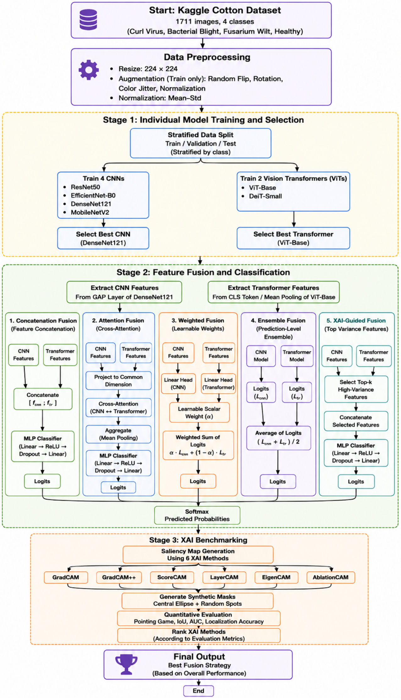
To ensure a fair comparison among the investigated backbone networks, identical optimization settings were employed for all individual models, including ResNet50, EfficientNet-B0, DenseNet121, MobileNetV2, ViT-Base, and DeiT-Small. Specifically, all models were trained using the AdamW optimizer with an initial learning rate of $1\times {10}^{-4}$, a batch size of 8, weight decay of $1\times {10}^{-5}$, the ReduceLROnPlateau learning-rate scheduler (factor = 0.5, patience = 2), and early stopping with a patience of three epochs. Individual backbone networks were trained for 12 epochs, while the proposed fusion models were trained for 15 epochs.

All backbone models were initialized using ImageNet pretrained weights provided by the PyTorch torchvision library. The original classification layer of each network was replaced with a task-specific classification head corresponding to the four cotton leaf disease classes, and the entire network was fine-tuned during training.

On the CPU-only system described in Table 4, the measured training time for the individual backbone models ranged from approximately 19 to 105 min per training run, depending on the architecture. Among the evaluated models, MobileNetV2 required the least training time (approximately 19 min), whereas ViT-Base required the longest (approximately 105 min), reflecting the higher computational requirements of the Transformer architecture. These measurements are representative of the training time observed across the evaluated backbone models.

To ensure full reproducibility, we set a fixed random seed of 42 for all experiments. The same seed was used for dataset splitting, model initialization, and bootstrap resampling. The model-selection procedure consisted of first training all individual CNN and Transformer models on the training set, evaluating them on the validation set, and selecting the best-performing CNN and Transformer based on validation accuracy. These selected backbones were then used as fixed feature extractors for all fusion models, which were trained and evaluated under identical conditions. The final best fusion model was selected based on test accuracy.

4.2. Evaluation Metrics

The following notation is used throughout the evaluation metrics: $TP$, $TN$, $FP$, and $FN$ denote true positives, true negatives, false positives, and false negatives, respectively. C represents the number of classes, while $T{P}_i$ and $F{N}_i$ indicate the true positives and false negatives for class i. For Cohen’s Kappa, $p_o$ denotes the observed agreement and $p_e$ represents the expected agreement by chance. In the ROC-based metrics, TPR and FPR denote the true positive rate and false positive rate, respectively. For XAI evaluation, H and M represent the heatmap and binary ground-truth mask, respectively.

Table 6. Summary of evaluation metrics used for classification performance, computational efficiency, and feature selection.

Metric	Description	Formula/Units
Classification Performance
Accuracy	Proportion of correct predictions	${\displaystyle \frac{TP+TN}{TP+TN+FP+FN}}$
Balanced Accuracy	Average recall per class	${\displaystyle {\displaystyle \frac{1}{C}}{\displaystyle \sum _{i=1}^C}{\displaystyle \frac{T{P}_i}{T{P}_i+F{N}_i}}}$
Precision (macro/weighted)	Weighted average of precision per class	${\displaystyle {\displaystyle \frac{1}{C}}{\displaystyle \sum _{i=1}^C}{\displaystyle \frac{T{P}_i}{T{P}_i+F{P}_i}}}$
Recall (macro/weighted)	Weighted average of recall per class	${\displaystyle {\displaystyle \frac{1}{C}}{\displaystyle \sum _{i=1}^C}{\displaystyle \frac{T{P}_i}{T{P}_i+F{N}_i}}}$
F1-Score (macro/weighted)	Harmonic mean of precision and recall	$2·{\displaystyle \frac{\mathrm{Precision}·\mathrm{Recall}}{\mathrm{Precision}+\mathrm{Recall}}}$
Cohen’s Kappa	Agreement between predictions and ground truth	${\displaystyle \frac{p_o-p_e}{1-p_e}}$
MCC	Correlation coefficient for multi-class	${\displaystyle \frac{TP·TN-FP·FN}{\sqrt{(TP+FP)(TP+FN)(TN+FP)(TN+FN)}}}$
AUC (macro/weighted)	Area under the ROC curve	${\displaystyle {\int }_0^1\mathrm{TPR}\left(\mathrm{FPR}\right)d\mathrm{FPR}}$
95% Bootstrap CI	Confidence interval for accuracy	Percentile bootstrap (500 resamples)
Computational Efficiency
FLOPs	Floating-point operations per forward pass	Giga/Mega FLOPs (GFLOPs/MFLOPs)
Parameters	Number of trainable weights	Million/Thousand (M/K)
Inference Time	Time to process one image	Milliseconds (ms)
Model Size	Disk space occupied by model	Megabytes (MB)
Explainability (XAI) Metrics
Pointing Game	Accuracy of the max heatmap point within the ground-truth mask	${\displaystyle \frac{\mathrm{hit}}{\mathrm{total}}}$
Intersection over Union (IoU)	Overlap between binarised heatmap and mask	${\displaystyle \frac{|\mathrm{H}\cap \mathrm{M}|}{|\mathrm{H}\cup \mathrm{M}|}}$
AUC (heatmap vs. mask)	ROC AUC between heatmap intensities and binary mask	${\displaystyle {\int }_0^1\mathrm{TPR}\left(\mathrm{FPR}\right)d\mathrm{FPR}}$
Localization Accuracy	Coverage of top-20% heatmap regions inside mask	${\displaystyle \frac{\sum {\mathrm{H}}_{\mathrm{top}20}·\mathrm{M}}{\sum \mathrm{M}}}$

summarizes the diverse set of metrics used in this work, their descriptions, and the corresponding formula or unit.

4.3. Performance Evaluation

The experimental results demonstrate the effectiveness of the proposed CNN–Transformer fusion framework for cotton leaf disease classification. For the 95% bootstrap confidence intervals reported in the results tables throughout this section, we employed the percentile bootstrap method with 500 resampling iterations. In each iteration, we randomly sampled test set predictions with replacement at the individual image level, recomputed the accuracy on the resampled set, and then constructed the confidence bounds using the 2.5th and 97.5th percentiles of the resulting bootstrap distribution.

At first, we evaluated the effectiveness of six different DL architectures, namely four CNNs and two Transformer-based neural networks. The detailed classification performance is reported in

Table 7. Classification performance of individual deep learning models. Performance metrics include Accuracy (Acc.), 95% Confidence Interval lower bound (CI L), 95% Confidence Interval upper bound (CI H), Balanced Accuracy (Bal.), Macro Precision (P(M)), Weighted Precision (P(W)), Macro Recall (R(M)), Weighted Recall (R(W)), Macro F1-score (F1(M)), Weighted F1-score (F1(W)), Cohen’s Kappa ($\kappa$), Matthews Correlation Coefficient (MCC), Macro Area Under the Receiver Operating Characteristic Curve (AUC(M)), and Weighted Area Under the Receiver Operating Characteristic Curve (AUC(W)).

Model	Acc.	CI L	CI H	Bal.	P(M)	P(W)	R(M)	R(W)	F1(M)	F1(W)	Kappa	MCC	AUC(M)	AUC(W)
CNN-ResNet50	85.96	81.3	91.2	85.87	0.8659	0.8648	0.8587	0.8596	0.8590	0.8589	0.8127	0.8147	0.9673	0.9671
CNN-EfficientNet-B0	91.81	87.7	95.3	91.75	0.9179	0.9182	0.9175	0.9181	0.9176	0.9181	0.8908	0.8908	0.9875	0.9876
CNN-DenseNet121	92.40	88.3	96.2	92.34	0.9262	0.9264	0.9234	0.9240	0.9237	0.9241	0.8986	0.8993	0.9858	0.9859
CNN-MobileNetV2	90.06	85.4	94.7	90.04	0.9016	0.9017	0.9004	0.9006	0.8997	0.8999	0.8674	0.8682	0.9815	0.9814
Transformer-ViT-Base	96.49	93.0	98.8	96.43	0.9648	0.9650	0.9643	0.9649	0.9642	0.9646	0.9532	0.9534	0.9994	0.9995
Transformer-DeiT-Small	87.13	82.1	91.8	87.10	0.8885	0.8881	0.8710	0.8713	0.8731	0.8732	0.8284	0.8328	0.9818	0.9819

, while the computational characteristics of the individual models are summarized in

Table 8. Computational complexity analysis of individual deep learning models.

Model	FLOPs	Parameters	Inference Time (ms)	Model Size (MB)
CNN-ResNet50	4.132 G	23.516 M	140.33	89.91
CNN-EfficientNet-B0	413.870 M	4.013 M	57.13	15.47
CNN-DenseNet121	2.896 G	6.958 M	149.67	26.86
CNN-MobileNetV2	326.212 M	2.229 M	40.67	8.63
Transformer-ViT-Base	16.848 G	85.611 M	346.87	327.31
Transformer-DeiT-Small	4.241 G	21.572 M	106.07	82.66

.

Out of all the individual models, Transformer-ViT-Base showed the best results in terms of accuracy with values of $96.49\%$ for accuracy, $0.9642$ for the macro F1 score, $0.9534$ for MCC, and $0.9995$ for weighted AUC. This proves the excellent representational learning capability of Transformer architectures for complex disease recognition tasks. In contrast, CNN-based models demonstrated comparatively lower performance, although DenseNet121 and EfficientNet-B0 achieved competitive results with accuracies above 90%. MobileNetV2 exhibited the lowest computational complexity, making it suitable for lightweight deployment scenarios. However, this reduction in complexity was accompanied by a moderate decrease in classification performance. Although ViT-Base achieved the best predictive performance among all individual models, it also incurred the highest computational cost and an inference time of $346.87$ ms.

The detailed classification performance and computational complexity analysis of the fusion models are presented in

Table 9. Classification performance of the proposed fusion strategies. Performance metrics include Accuracy (Acc.), 95% Confidence Interval lower bound (CI L), 95% Confidence Interval upper bound (CI H), Balanced Accuracy (Bal.), Macro Precision (P(M)), Weighted Precision (P(W)), Macro Recall (R(M)), Weighted Recall (R(W)), Macro F1-score (F1(M)), Weighted F1-score (F1(W)), Cohen’s Kappa ($\kappa$), Matthews Correlation Coefficient (MCC), Macro Area Under the Receiver Operating Characteristic Curve (AUC(M)), and Weighted Area Under the Receiver Operating Characteristic Curve (AUC(W)).

Fusion Approach	Acc.	CI L	CI H	Bal.	P(M)	P(W)	R(M)	R(W)	F1(M)	F1(W)	$\mathit{\kappa }$	MCC	AUC(M)	AUC(W)
Concatenation Fusion	99.42	98.2	100	99.40	0.9942	0.9943	0.9940	0.9942	0.9940	0.9942	0.9922	0.9922	0.9999	0.9999
Attention Fusion	97.08	94.7	99.4	97.10	0.9717	0.9722	0.9710	0.9708	0.9709	0.9710	0.9610	0.9613	0.9996	0.9996
Weighted Fusion	95.32	91.8	98.2	95.28	0.9531	0.9532	0.9528	0.9532	0.9528	0.9531	0.9376	0.9377	0.9979	0.9980
Ensemble Fusion	97.66	95.3	99.4	97.66	0.9770	0.9774	0.9766	0.9766	0.9765	0.9767	0.9688	0.9690	0.9998	0.9998
variance-based fusion	98.83	97.1	100	98.81	0.9884	0.9886	0.9881	0.9883	0.9880	0.9882	0.9844	0.9845	0.9997	0.9997

and

Table 10. Computational complexity analysis of the proposed fusion models.

Fusion Approach	FLOPs	Parameters	Inference Time (ms)	Model Size (MB)
Concatenation Fusion	19.745 G	93.612 M	552.74	358.18
Attention Fusion	19.744 G	93.055 M	516.54	357.06
Weighted Fusion	19.744 G	92.569 M	503.00	354.20
Ensemble Fusion	19.744 G	92.569 M	500.81	354.17
variance-based fusion	19.744 G	92.733 M	557.74	354.83

, respectively. The fusion results demonstrated substantial performance improvements over all standalone architectures, confirming that CNN and Transformer representations provide complementary discriminative information. In particular, the concatenation fusion strategy achieved the best overall performance with an accuracy of $99.42\%$, macro F1-score of $0.9940$, MCC of $0.9922$, and weighted AUC of $0.9999$.

To ensure full transparency, we examined the exact classification outcomes for the best-performing Concatenation Fusion model. Out of the 171 test samples, 170 were correctly classified, and only 1 was misclassified, yielding an accuracy of 99.42%. The single error corresponded to a healthy leaf sample that was incorrectly predicted as curl_virus. This near-perfect classification performance is consistent with the bootstrapped 95% confidence interval of 98.2–100.0% reported in Table 9 and confirms the robustness of the proposed fusion approach.

The variance-based fusion strategy also achieved highly competitive performance with an accuracy of $98.83\%$ and MCC of $0.9845$, demonstrating that explainability-driven feature refinement can effectively reduce redundant representations while preserving highly informative disease-related features. Similarly, the ensemble fusion strategy achieved strong classification performance with an accuracy of $97.66\%$, suggesting that prediction-level aggregation improves robustness and generalization. In contrast, weighted fusion exhibited comparatively lower performance than feature-level fusion methods, indicating that directly combining logits may not fully exploit the complementary spatial and contextual representations learned by CNN and transformer backbones.

Although the fusion approaches significantly improved classification performance, they also introduced higher computational complexity due to the simultaneous utilization of dual backbones. All fusion models required approximately $19.7$G FLOPs and more than 92M trainable parameters. Among the fusion strategies, ensemble fusion achieved the lowest inference time of $500.81$ ms, while the variance-based fusion model exhibited the highest inference cost because of the additional feature refinement operations. Nevertheless, the substantial improvement in predictive performance justifies the increased computational overhead, particularly for high-accuracy agricultural disease diagnosis systems.

It is important to note that for computational complexity analysis, the parameter counts and FLOPs were calculated for the final model architectures used in the experiments. For each pretrained backbone, the original ImageNet classification head was replaced with the task-specific classification layer before training. Accordingly, the reported computational statistics for the fusion models include the parameters and operations of both modified backbone networks together with the additional fusion and task-specific classification layers, where applicable. The reported counts (Table 8 and Table 10) therefore do not represent the original ImageNet models with their original classification heads.

Overall, the obtained results confirm that integrating CNN-based local feature extraction with Transformer-based global contextual modeling substantially improves cotton leaf disease classification performance. The proposed fusion framework consistently outperformed all standalone architectures across all evaluation metrics, while the concatenation fusion strategy achieved the best balance between discriminative capability and classification robustness. These findings demonstrate the effectiveness of hybrid CNN–Transformer learning for intelligent agricultural disease diagnosis systems.

4.4. Explainability Analysis

To investigate how different explainability techniques identify disease-relevant regions while suppressing irrelevant background information, we performed a qualitative comparison using six widely adopted XAI methods: GradCAM, GradCAM++, ScoreCAM, LayerCAM, EigenCAM, and AblationCAM. We selected representative samples from the cotton leaf disease dataset to visually examine the spatial distribution of model attention.

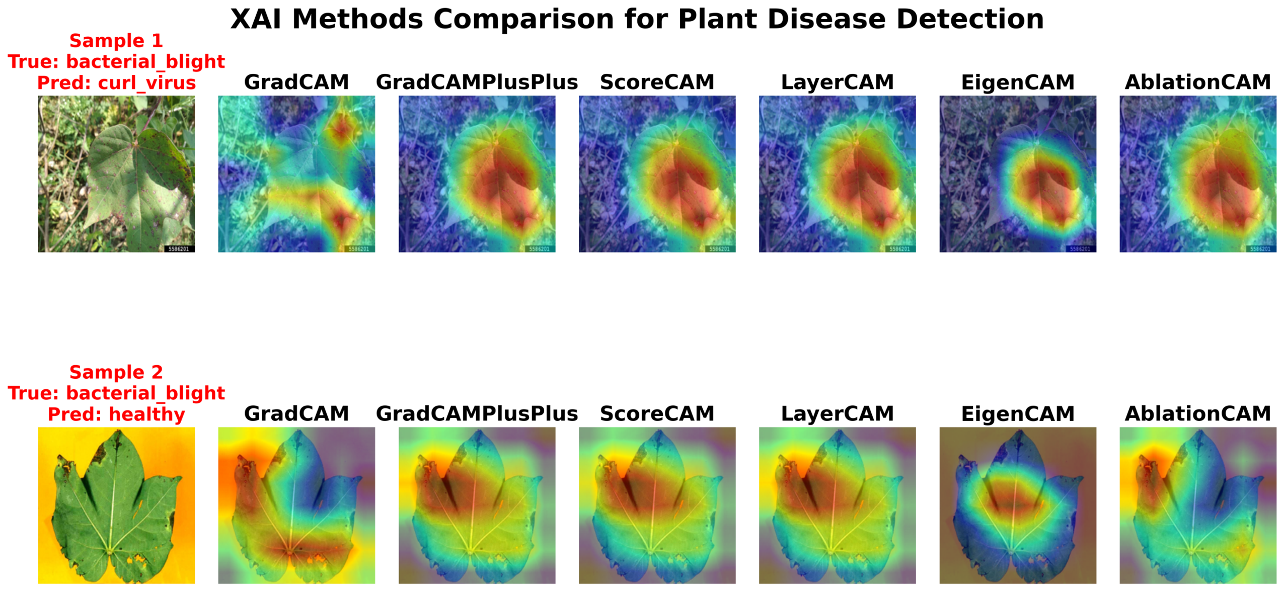
Figure 3 presents the explanation maps generated by the six approaches for three representative test images, all correctly classified as bacterial blight. The figure is organized with each row corresponding to a test sample, and columns displaying the original image, followed by the heatmaps from each XAI method.

There is one important observation that can be made about background suppression after performing qualitative analysis. Techniques like GradCAM, GradCAM++, ScoreCAM, LayerCAM, and AblationCAM consistently resulted in activation maps that overlapped into the background area. The presence of this noise showed that the methods do, at times, give high importance to areas that are not leaf parts, thus making their explanations for localizing the diseases inconsistent. However, the EigenCAM algorithm produces very restricted and accurate activation maps only within the leaf area. By producing zero or negligible attention outside the leaf area, EigenCAM effectively eliminates false-positive attributions from the background.

Even though these models have background leakage, GradCAM++ and ScoreCAM have sharper activations of the lesion-specific features within the leaf, but their inability to eliminate the background interference means that they are not suitable for exact mapping of the disease. The EigenCAM model is the best since it combines both plant anatomy and lesion features. This behavior suggests that EigenCAM inherently captures the model’s spatial grounding more faithfully, making it particularly suitable for plant disease detection where distinguishing the target object (the leaf) from the background is essential for trustworthy explanations.

Overall, while GradCAM++ and ScoreCAM provide strong intra-leaf localization, EigenCAM outperforms them in terms of spatial contextuality by avoiding irrelevant background activations. The quantitative metrics reported in the bottom table further substantiate these visual observations.

Furthermore, to objectively assess the localization performance of the six XAI methods, we performed a quantitative evaluation using four complementary metrics: Pointing Game, IoU, AUC, and localization accuracy. These metrics evaluate different aspects of explanation quality: Pointing Game measures whether the maximum activation falls within the ground-truth region; IoU quantifies spatial overlap between binarized explanations and disease regions; AUC assesses the overall ranking of pixel importance; and Localization Accuracy measures the coverage of ground-truth regions by the top-k% most activated pixels.

Table 11. Average quantitative metrics for six XAI methods across all test samples. Bold values indicate the best performance for each metric.

Method	Pointing Game	IoU	AUC	Localization Accuracy
GradCAM	0.583	0.330	0.674	0.336
GradCAM++	0.500	0.451	0.742	0.413
ScoreCAM	0.417	0.435	0.750	0.413
LayerCAM	0.417	0.433	0.748	0.441
EigenCAM	0.750	0.457	0.806	0.613
AblationCAM	0.500	0.322	0.638	0.301

presents the average performance of each method across all test samples. The results reveal distinct performance characteristics across methods, with EigenCAM consistently achieving the highest scores in the most critical metrics.

EigenCAM exhibits superior performance compared to other methods based on all four criteria and proves its ability to localize diseases more precisely. EigenCAM scores 0.750 in the Pointing Game criterion, meaning that in 75% of test cases, this method is able to detect the most discriminative part of the disease location area. This method significantly outperforms GradCAM and AblationCAM, scoring 0.583 and 0.500, respectively. However, EigenCAM achieves the best IoU (0.457), AUC (0.806), and Localization Accuracy (0.613), implying that the attention maps generated by it not only successfully localize the areas affected by diseases but also maintain fine-grained alignment with the ground truth.

While gradient-based algorithms like GradCAM and GradCAM++ utilize the propagation of gradients through the network which are themselves subject to problems related to noisy and vanishing gradients, EigenCAM calculates the first principal component of the activations of the target convolutional layer. In doing so, it extracts the most prominent variation in the feature space, thus successfully filtering out any background noise to concentrate only on the most discriminative features. As a result, the explanation maps produced by EigenCAM are extremely precise and contextually accurate due to their high scores.

GradCAM++ and ScoreCAM exhibit competitive performance, particularly in terms of AUC (0.742 and 0.750, respectively) and IoU (0.451 and 0.435). GradCAM++ ranks second to the highest IoU, implying that the gradient weighting method used by GradCAM++ produces attention maps with high spatial agreement with the diseased regions. ScoreCAM, where gradients are replaced by forward pass perturbation scores, performs very well in ranking pixel importance (AUC = 0.750).

LayerCAM and GradCAM fall somewhere in the middle, with GradCAM obtaining the best score of the Pointing Game (0.583) among all approaches except EigenCams, whereas IoU and localization accuracy scores (both 0.330) remain quite low for GradCAM. It indicates that while GradCAM correctly locates the correct region most of the time, its attention regions usually tend to be large and not as precisely located around the lesion boundaries.

Among all models, the AblationCAM demonstrates the worst result by showing the smallest IoU (0.322), AUC (0.638), and localization score (0.301). Such a result can be caused by the fact that AblationCAM uses iterative ablation of the feature maps and, therefore, is sensitive to the perturbation methods used.

Ranking results shown in

Table 12. Ranking of XAI methods based on combined performance across all four metrics. The combined score is computed as the average of normalized metric values.

Rank	Method	Combined Score
1	EigenCAM	0.906
2	GradCAM++	0.707
3	ScoreCAM	0.700
4	LayerCAM	0.695
5	GradCAM	0.682
6	AblationCAM	0.564

represent an integrated approach that takes into account all four criteria altogether. EigenCAM becomes the clear leader with an overall score of 0.906, outperforming GradCAM++ by a wide margin (GradCAM++ achieves second place with a value of 0.707).

Interestingly, the qualitative observations align well with the quantitative findings. EigenCAM’s strict confinement of attention to leaf surfaces, as visually observed in Figure 3, is quantitatively validated by its superior IoU and localization accuracy scores. The background leakage observed in GradCAM, GradCAM++, ScoreCAM, LayerCAM, and AblationCAM is reflected in their lower IoU values, as the spurious background activations reduce the spatial overlap with ground-truth disease regions.

These findings have significant implications for the selection of appropriate XAI techniques in agricultural AI applications. Although GradCAM-based techniques are commonly used on account of their ease and efficiency, the thorough analysis conducted by us reveals that EigenCAM is far superior in terms of reliability and accuracy. EigenCAM is well suited for practical applications where plants are often photographed within their natural environment because of its capacity to ignore background distractions while still being highly sensitive to disease-related features. The method’s inherent ability to capture the most salient feature variations through principal component analysis provides a principled approach to explainability that is less susceptible to the limitations of gradient-based or perturbation-based methods. In summary, the quantitative evaluation establishes EigenCAM as the most effective XAI method for cotton leaf disease classification, achieving superior performance across all evaluated metrics.

5. Discussion

The experimental findings yield a number of important conclusions concerning the effectiveness of CNN–Transformer fusion, the significance of different fusion techniques, and the practical application of XAI-based approaches to classification of cotton leaf diseases. In contrast to earlier studies where emphasis is placed on the development of new hybrid models, this study evaluates various fusion methods within one experimental setup. In conclusion, the major contribution of this study is therefore not the introduction of a fundamentally new CNN, Transformer, fusion, or XAI algorithm, but the systematic empirical investigation of established fusion strategies and explainability methods under a unified experimental protocol.

5.1. Interpretation of CNN–Transformer Fusion Performance

The higher efficiency of the concatenation method of fusion is possible due to the property of maintaining complementarity between CNN and Transformer-based representations. Indeed, CNNs possess natural advantages in identifying local spatial relationships within images in terms of textures, lesions, and other fine disease structure information. In contrast, Transformers learn dependencies across the image areas by means of self-attention processes. Thus, using the simple concatenation of the output of DenseNet121 and ViT-Base models, we maintain all the information in both feature spaces without any additional assumptions concerning feature weights. This observation explains why concatenation fusion achieved the highest classification performance, obtaining an accuracy of 99.42%, MCC of 0.9922, and weighted AUC of 0.9999.

Contrarily, attention-based fusion performed poorly (97.08%), despite being an adaptable method of feature combination. This indicates that for this particular dataset of cotton diseases, learning selective interactions between CNN and Transformer features leads to inhibition of some information that would otherwise be helpful for classification. Similarly, weighted prediction fusion and ensemble fusion operate at the decision level rather than the feature representation level. While this makes them more reliable, they fail to explore the interaction between low-level spatial features and high-level contextual features.

The variance-based feature fusion strategy achieved competitive performance (98.83%), demonstrating that reducing redundant feature dimensions can preserve most discriminative information. However, its slightly lower accuracy compared with full feature concatenation suggests that some discarded high-variance-independent features may still contribute useful information for disease discrimination. These findings highlight that feature reduction strategies should carefully balance computational efficiency and information preservation.

Overall, the results have shown that the success of using CNN–Transformer fusion is not only a matter of combining two different neural architectures, but also a matter of retaining complementary feature representation created by these architectures. The results reveal that a simple fusion at the feature level could lead to high performance when the aim is to achieve optimal classification performance, whereas more selective fusion mechanisms may become advantageous when computational constraints are prioritized.

5.2. Explainability Performance and Practical Implications

Quantitative XAI Evaluation shows that various techniques have different localization abilities. Though gradient-based techniques like GradCAM and GradCAM++ are widely used due to their simplicity and fast processing, the results show that EigenCAM is the most precise one for localization among all others for the cotton disease recognition problem. EigenCAM reached the highest values of all scores combined (0.906), as well as of Pointing Game score (0.750), Intersection over Union (IoU) (0.457), Area Under Curve (AUC) (0.806), and Localization Accuracy (0.613).

EigenCAM’s superiority in performance may be attributed to the activation-based approach employed by it since it involves the extraction of the principal component from the feature activations as opposed to the use of gradients for propagation. Hence, EigenCAM will be immune to noise in the gradient and will produce more reliable activation maps, especially when considering images of agriculture where there are changes in background, lighting, and leaves.

However, it should be noted that GradCAM++ and ScoreCAM have shown comparable localization results as well, especially in terms of IoU and AUC scores. The use of such methods is quite beneficial for cases where computational simplicity and compatibility with already trained CNN models are highly desired. Taking into consideration the practical aspect of agriculture, the explanation of the model decision is very important since it provides an opportunity to ensure that the model concentrates on biologically significant symptoms of the disease, rather than other features of the picture.

It is important to note that the quantitative XAI assessment in this work was performed using synthetic reference masks because publicly available pixel-level lesion annotations for the studied cotton leaf dataset were unavailable. Although these masks provide a consistent and uniform evaluation framework, their simplified geometric structure and spatial distribution may introduce evaluation bias and may favor XAI methods whose activation patterns overlap more closely with the constructed reference regions. In particular, they may not adequately represent the irregular lesion boundaries, variable severity levels, and heterogeneous spatial distributions observed in real cotton leaf diseases. Therefore, the resulting XAI rankings, including the superior performance observed for EigenCAM, should be interpreted as preliminary evidence under the present evaluation setting rather than definitive confirmation of real-world disease-localization superiority. Future studies should validate these findings using representative subsets of images with pixel-level lesion masks annotated or verified by agricultural domain experts.

5.3. Accuracy, Computational Cost, and Deployment Considerations

From the findings of the experiments, there is an observable trade-off between the performance of the predictions and computation. The most accurate concatenation fusion method had considerably better prediction accuracy compared to the CNN and Transformer models individually; however, this was attained through an increase in the complexity of computations. Particularly, the dual backbone fusion system utilizes 19.7 GFLOPs, more than 93 million parameters, and takes 552.74 ms for inference per image using the presented CPU configuration. In contrast, the MobileNetV2 takes 40.67 ms and uses 2.23 million parameters. Although the concatenation fusion model improves the classification accuracy from 90.64% for MobileNetV2 to 99.42%, this gain of 8.78 percentage points comes at the cost of approximately $13.6\times$ higher CPU inference latency and substantially greater model complexity. Therefore, whether this trade-off is justified depends on the deployment scenario: the additional accuracy may be valuable in cloud-based or expert-assisted diagnostic systems where reliability is prioritized, whereas MobileNetV2 or other lightweight alternatives may be more suitable for real-time, resource-constrained field deployment.

Based on the results, it can be stated that the proposed framework is more appropriate to be used in those areas where there is a need to focus more on prediction performance and explainability of the model, such as a cloud-based farming support system or any system that involves disease identification using experts’ help. In contrast, resource-constrained field devices may require lightweight alternatives. For practical deployment on edge devices, future optimization strategies such as knowledge distillation, model pruning, quantization, and lightweight CNN–Transformer architectures could reduce computational requirements while maintaining acceptable diagnostic accuracy.

The use of ImageNet-based transfer learning should also be taken into account when scaling the proposed framework to novel agricultural applications. The benefits of transfer learning are obvious in situations where labeled agricultural data is limited, but the disparity between natural images and plant pathology images could have an impact on generalization. Future research should investigate self-supervised agricultural pre-training strategies and cross-domain adaptation approaches to reduce dependency on generic ImageNet representations.

5.4. Limitations and Future Research Directions

First, the experiments were conducted on a single dataset containing 1711 images, with 171 images reserved for the independent test set. Although stratified splitting and a separate test set were used, the relatively limited dataset size and the high capacity of the dual-backbone fusion model may increase the risk that the reported 99.42% accuracy is influenced by dataset-specific characteristics, including background, illumination, acquisition conditions, or other non-pathological visual cues. In addition, because the publicly available dataset does not provide plant-level or acquisition-session identifiers, complete separation of potentially correlated images across the subsets could not be verified, and the possibility of near-duplicate images cannot be completely excluded. Therefore, the current results should be interpreted as strong performance on the studied dataset rather than definitive evidence of broad real-world generalization. Future studies should validate the proposed framework using larger and independently collected datasets, stratified cross-validation, multiple geographical regions, and acquisition settings with appropriate plant-level or session-level separation.

Second, the proposed dual-backbone system is more computationally expensive than lightweight CNN systems. Even though the added complexity yields better classification accuracy and feature representation, future research should focus on developing more efficient hybrid architectures suitable for real-time field deployment.

Third, the present model considers only visual disease classification. In real agricultural fields, there are many different factors that contribute to the onset of diseases, which include climatic conditions, soil types, and the passage of time. Integrating visual information with environmental and temporal data may enable more comprehensive disease monitoring and early risk prediction systems.

Fourth, the investigated backbone models rely on ImageNet-pretrained weights through transfer learning. Although this initialization facilitates effective learning from the relatively limited cotton disease dataset, the learned representations originate from a natural-image domain and may not fully capture crop- and disease-specific characteristics. Consequently, the performance and adaptation efficiency of the proposed framework may depend on the compatibility between the source-domain representations and the target agricultural domain. Future research should therefore investigate domain-specific pretraining, self-supervised learning on large-scale agricultural imagery, and training strategies that reduce dependence on generic ImageNet representations.

Finally, although the presented XAI analysis provides quantitative evidence for comparing explanation methods, validation with expert-provided lesion annotations remains an important future direction. Furthermore, the applicability of the proposed framework to other crop species has not been experimentally validated in the present study. Differences in leaf morphology, disease appearance, imaging conditions, and symptom characteristics across crops may affect both classification performance and the behavior of the XAI methods. Therefore, evaluation on diverse crop species and disease datasets is necessary to determine whether the observed performance and explainability characteristics generalize beyond cotton.

6. Conclusions

In this study, we presented a systematic empirical framework for evaluating CNN–Transformer fusion and explainability strategies for cotton leaf disease classification. Rather than proposing a fundamentally new CNN, Transformer, fusion mechanism, or XAI algorithm, the primary contribution of this work is the controlled comparison of established approaches under a unified experimental protocol. By keeping the backbone models fixed while evaluating multiple fusion strategies, computational characteristics, and XAI methods, the study provides empirical evidence regarding the relative effectiveness, efficiency, and explainability of these approaches for agricultural disease classification.

Through extensive experimentation on the Kaggle cotton leaf disease dataset, we demonstrated several key findings. First, among individual architectures, ViT-Base achieved superior performance ($96.49\%$ accuracy) compared to the best CNN model, DenseNet121 ($92.40\%$), highlighting the advantage of global contextual modeling for plant disease recognition. However, CNN architectures remain valuable for capturing fine-grained local disease characteristics, with EfficientNet-B0 demonstrating an excellent trade-off between accuracy ($91.81\%$) and computational efficiency ($57.13$ ms inference time, $15.47$ MB model size).

Second, our systematic evaluation of five fusion strategies revealed that simple feature concatenation of CNN and transformer representations achieved the highest classification performance ($99.42\%$ accuracy, 95% CI: $98.2$–$100\%$, MCC = $0.9922$) and outperformed all standalone models. The concatenation strategy’s effectiveness can be attributed to its ability to preserve the full representational capacity of both architectures without imposing restrictive assumptions about feature interactions. The proposed variance-based fusion method, which retains only the top $30\%$ most variable features, achieved an accuracy of $98.83\%$. This means it is possible to eliminate redundant features through the XAI process without sacrificing discriminative power.

Third, our extensive computational analysis showed that there are certain trade-offs involved when deploying in real life. Although fusion models offer better performance in terms of accuracy, they also come with a huge amount of computational cost (around $19.7$ GFLOPs, >92M parameters, and 500–558 ms inference time) compared to lightweight CNN models such as MobileNetV2 (326 MFLOPs, $2.23$M parameters, $40.67$ ms). These results offer practical insights into choosing the right architecture given the deployment restrictions, from resource-limited edge devices to high performance cloud-based inference solutions.

Fourth, using one of the first benchmarking efforts on XAI approaches for cotton leaf disease detection, we show that EigenCAM consistently outperforms gradient approaches on all considered metrics (Pointing Game: $0.750$, IoU: $0.457$, AUC: $0.806$, Localization Accuracy: $0.613$). This finding has important implications for the selection of explanation methods in precision agriculture, where the reliability of visual explanations directly impacts stakeholder trust and adoption.

The practical implications of our findings extend beyond cotton disease detection. The proposed framework’s dual-backbone architecture and rigorous evaluation methodology can be readily adapted to other agricultural disease diagnosis tasks, crop monitoring systems, and plant phenotyping applications where both local lesion characteristics and global contextual information are essential for accurate diagnosis. The quantitative XAI benchmarking framework provides a reproducible methodology for evaluating explanation quality across different tasks and datasets, addressing a critical gap in the agricultural AI literature.

Despite the promising results, several limitations need to be acknowledged. The dataset, while representative of real-field conditions with variations in illumination, background, and disease severity, is relatively modest in size (1711 images). Although we employed data augmentation and TL to mitigate overfitting, the framework’s generalization to larger and more diverse datasets, multiple growing seasons, and geographical regions remains to be validated. Moreover, the artificial ground-truth masks employed to assess the XAI models could potentially lack sufficient consideration of the irregular nature of the lesions caused by natural infections. The use of experts’ annotations of disease regions at the pixel level would be recommended in future research on validating the XAI benchmarking outcomes.

Future research will focus on extending the framework toward multi-temporal disease progression analysis and multi-class severity grading, while developing lightweight hybrid model variants optimized for real-time and edge deployment through knowledge distillation, network quantization, and efficient feature fusion. We also plan to investigate multimodal agricultural intelligence by integrating visual features with local meteorological, soil, and temporal information for more comprehensive and proactive disease risk assessment. In addition, the proposed framework and XAI benchmarking methodology will be evaluated across diverse cotton datasets and extended to other crop and plant disease classification tasks to assess its cross-crop generalization. Structurally, adaptive fusion mechanisms, including dynamic routing and mixture-of-experts architectures, will be explored to improve the balance between predictive performance and computational efficiency. Finally, user studies with agricultural experts will be conducted to evaluate the practical utility, interpretability, and trustworthiness of the generated explanations under realistic field conditions.