Co-Management of Communication and Computational Energy in Wirelessly Connected Mobile Robots

Abstract

Battery-powered mobile robots that rely on an edge server for perception spend energy in three places at once: the on-board processor, the radio front end and the drivetrain. These budgets are normally optimised separately, which is a mistake, as lowering the processor clock pushes work onto the wireless link, transmitting into a poor channel costs far more than waiting for a better one, and where the robot drives determines what the channel will be. We formulate the co-management of all three as a minimisation of long-run average energy for a fleet sharing an access point and subject to task deadlines, a power budget and a mission-progress constraint that forces every policy under comparison to cover the same ground. The resulting stochastic mixed-integer non-convex program is made tractable by a Lyapunov drift-plus-penalty argument that decomposes it into four per-slot subproblems: a square-root clock rule, a water-filling transmit-power rule with an explicit on/off test, a join-the-shorter-queue offloading split, and a short lookahead over admissible speeds. The policy needs no channel or workload statistics and attains an A per-task deadline mechanism, feasibility floors on the clock and transmit decisions, and closes the gap between queue-stability guarantees and individual task deadlines, which drift arguments alone do not bound. The policy needs no channel or workload statistics and attains an $\left[O\right(1/V),O(V\left)\right]$ energy–delay tradeoff, stated under precisely qualified assumptions. In a per-task simulation study against six baselines, the policy reduced combined communication and computation power by 25% relative to the strongest deadline-compliant baseline ($p<{10}^{-4}$) at equal mission progress, and was the only scheme to hold deadline violations below 0.5% across the full load range, where every baseline exceeded 16% at high load.

1. Introduction

A warehouse robot running visual odometry, obstacle segmentation and a local planner is, from the point of view of its battery, three appliances in one chassis. The drivetrain moves it. The processor turns sensor frames into a model of the world. The radio keeps it in touch with whatever infrastructure it depends on. Each of these has been studied hard on its own. Motion planners that minimise mechanical work are a mature topic; dynamic voltage and frequency scaling (DVFS) has been standard practice in embedded processors for two decades; and the wireless community has produced extensive literature on energy-efficient transmission. What has received much less attention is the fact that on a robot these three budgets are strongly coupled, and that optimising them separately forgoes substantial energy savings.

The coupling is easy to state. Suppose a robot must process a 2 $\mathrm{M}$$\mathrm{bit}$ sensor frame every 100 $\mathrm{m}$$\mathrm{s}$. It can do the work on board, in which case the processor must run near its maximum clock, and the dynamic power, which grows roughly with the cube of the frequency, becomes the dominant term. Or it can ship the frame to an edge server, in which case the processor idles but the radio must sustain several megabits per second. The cost of doing that depends entirely on the channel. At a favourable position a few milliwatts suffice; in a shadowed corner of the same building, the same throughput may require the full transmit budget, or may be unattainable at any power. And the channel is not exogenous, because the robot is the thing that moves. A path that is two metres longer but stays in the line of sight of the access point can be cheaper overall than the geometrically shortest one, even after paying for the extra locomotion.

Existing work tends to cut through this in one of two ways. The mobile edge computing (MEC) literature treats the device as a stationary or arbitrarily moving user, and optimises the offloading decision jointly with the radio resources. It takes the mobility as given, however, and ignores the mechanical energy entirely [1,2]. The robotics literature, conversely, has produced sophisticated energy-aware planners that treat communication as either free or as a hard connectivity constraint. Both simplifications are reasonable in their own settings. Neither is adequate for a battery-limited robot whose perception pipeline is heavy enough that the computation and communication terms are comparable to the locomotion term, which, as the measurements in recent field studies suggest, is increasingly the normal case rather than an exotic one [3].

This paper takes the position that communication energy and computational energy on a mobile robot should be managed by a single controller, and that the robot’s own motion belongs in the same loop. We call this co-management. The contribution is not a new offloading heuristic but a formulation in which the three budgets appear as arguments of one objective, together with an online algorithm that solves it without requiring any statistics of the channel or the workload.

1.1. Contributions

The paper makes three contributions.

(1) A three-domain co-management formulation and its decomposition. We formulate the joint management of processor, radio and drivetrain energy for a robot fleet as one long-run average minimisation subject to task-deadline, power, bandwidth and mission-progress constraints (Section 4), and show that although the problem is stochastic, non-convex and mixed-integer, a Lyapunov argument decomposes it into four per-slot subproblems that are solvable in closed form or by small enumeration (Section 5). Relative to the established Lyapunov offloading literature [4,5,6,7,8,9,10], which optimises computation against communication for a device whose mobility is exogenous, the novelty is not the drift machinery but what enters the drift: a third, controlled decision variable (speed) that shapes the channel process itself, and a mission-progress virtual queue that makes the resulting comparison well posed. The consequences are technical as well as conceptual—the standard i.i.d. optimality argument no longer applies unmodified, and Section 5 states precisely what survives (stability unconditionally; near-optimality relative to a fixed speed profile) rather than asserting the usual bound.

(2) Per-task deadline enforcement, which drift arguments do not provide. Mean-rate stability bounds time-average backlogs, not the tails that a control loop actually cares about, and we show the gap is real rather than theoretical: the unguarded drift-minimising rules strand individual tasks for tens of seconds while every time-average looks healthy. Section 5.6 adds explicit per-task feasibility floors on the clock and transmit decisions, which hold measured violations below 0.5% across the load range. This also reveals a regime the unconstrained theory does not describe: beyond a critical V the floors become the binding control and energy rises with V instead of falling.

(3) A per-task evaluation of the single-AP algorithm, reported with its negative results. Against eight baselines, with end-to-end latency accounted per task, confidence intervals, significance tests, ablation and sensitivity, we show the algorithm of contributions (1)–(2) cuts communication and computation power by 25% against the strongest deadline-compliant baseline while holding violations below 0.5% where every baseline exceeds 16%, and we report what did not work alongside what did: the channel-lookahead term contributes no measurable saving in this scenario class, and the deadline machinery degrades under bursty arrivals. Beyond this core result, Section 6 additionally reports two generality checks rather than further contributions: the formulation extends to multi-AP, multi-edge deployment without algorithmic change, and the routing rule remains preferable to two learned alternatives. These checks establish scope, not novelty, and are reported as such. The complete simulator, seeds and configurations are released, and every figure regenerates from them.

1.2. Organisation

Section 2 reviews the relevant literature and identifies the gap. Section 3 sets up the system model, including the three energy models and the queueing dynamics. Section 4 states the optimisation problem and explains why it is hard. Section 5 develops the co-management algorithm and analyses it. Section 6 reports the evaluation. Section 7 discusses what the results do and do not establish, along with the limitations of the study, and Section 8 concludes the paper.

2. Related Work

2.1. Computation Offloading and Mobile Edge Computing

The idea that a resource-poor device can save energy by sending work to a better-provisioned machine predates edge computing by some margin. Kumar and Lu framed the question sharply, offloading pays only when the communication cost is smaller than the computation cost avoided, which is a statement about the ratio of data volume to computational intensity [11]. MAUI [12] and CloneCloud [13] turned this into working systems that partition applications at run time, and Miettinen and Nurminen provided the measurements that anchored the energy models everyone subsequently used [14]. Surveys by Dinh et al. [15] and, for the edge era, by Mao et al. [1], Mach and Becvar [2], Shi et al. [16], Taleb et al. [17] and Wang et al. [18] map the design space in detail.

A third perspective treats the radio access network itself as the object of energy optimisation. Cell-free architectures distribute many access points under joint control, and when they also carry a sensing function the resulting integrated sensing and communication (ISAC) system must allocate power across sensing and communication objectives at once; energy-efficient designs for cell-free ISAC serving urban air mobility are a recent instance, and they share with our problem both the structure of the objective, long-run energy minimisation under service-quality constraints, and the difficulty that the constraint set is non-convex [19]. The distinction is where the decision variables live. The literature optimises the infrastructure’s beamforming and power allocation for a given set of user demands; we optimise the terminal’s scheduling of its own three energy domains for a given infrastructure. The two compose naturally, and the multi-AP extension of Section 6.14 is precisely the point of contact: a cell-free deployment would supply the per-AP association and bandwidth structure that Section 6.14 adds by hand, and a robot fleet would supply the demand model such an infrastructure needs.

A complementary line of work attacks the communication energy problem at the physical layer rather than at the scheduler, either by improving the channel itself or by hardening it. Reconfigurable intelligent surfaces reshape the propagation environment, and self-powered absorptive designs do so under a harvested-energy budget, which makes the surface a net-zero addition to the link rather than another powered node [20]; distributed time-modulated arrays pursue a related goal at the transmitter, using time-modulation to shape radiation in angle and thereby to secure the link for distributed IoT nodes [21]. These techniques are orthogonal to, and composable with, what we do here: they alter the mapping from transmit power to achievable rate, the function $r_i\left(t\right)$ of (8), whereas our controller takes that mapping as given and decides how much power to spend and when. A deployment that improved the channel by such means would change the numerical value of the communication–computation exchange rate, and hence how much work the co-manager routes to the radio, but not the structure of any of the four subproblems. We regard the combination as a promising direction, particularly where security constraints make some links preferable to others and the routing rule of (24) would need a secrecy term alongside its energy and queue terms.

Within that space, the strand closest to our work is the joint optimisation of radio and computational resources. Wang et al. combined partial offloading with DVFS and showed that the two decisions interact [22]. Chen et al. analysed multi-user offloading as a game and established convergence to a Nash equilibrium [23]. Zhang et al. derived energy-optimal scheduling under a stochastic channel [24], and Huang et al. gave one of the earliest Lyapunov-based dynamic offloading algorithms [4]. Mao and co-authors extended the Lyapunov approach to energy-harvesting devices [5] and then to multi-user systems with joint radio and computational management [6], Kwak et al. solved a closely related problem with the same machinery [7], and Guo et al. added cooperative task scheduling [25]. Delay-optimal rather than energy-optimal scheduling was treated by Liu et al. [26].

Sardellitti et al. treated the joint radio-and-computation allocation as a non-convex program and solved it by successive convex approximation in the single-cell and then the multicell case [27], and Wang et al. derived the joint offloading and computing solution for wireless powered systems [28]. The Lyapunov strand has continued to develop: Guo et al. handled partial offloading with harvested energy [8], Tong et al. applied the same machinery to energy-saving offloading for IoT devices [9], and Bi et al. combined drift-plus-penalty with deep reinforcement learning, using the Lyapunov term to retain a stability guarantee that a purely learned policy would lack [10]. That last hybrid is philosophically close to what we do, in that it insists on keeping the guarantee.

Our per-slot subproblems for the processor and the radio are recognisably descendants of this line of work, and we make no claim of novelty for them individually. What is different here is the third dimension.

2.2. Energy in Mobile Robotics and Cloud Robotics

Cloud and edge robotics, offloading robot computation to remote infrastructure was surveyed by Kehoe et al. [29] and, more recently and with an edge emphasis, by Chowdhury and Parasuraman [30]. The systems concerns are well understood and ROS [31] has made the plumbing routine. The interesting question is when to offload, and here the robotics literature has produced answers that the MEC literature largely has not, because it takes mobility seriously.

The closest antecedents to our formulation are the papers of Rahman and colleagues, who explicitly incorporated motion and connectivity into the offloading decision, first for a single robot [32] and then for a multi-robot system with robot-to-robot sharing [33]. They solve the resulting problem with a multi-layer genetic algorithm. This is effective but offline: the decisions are computed for a known route against estimated bandwidth, and the method does not come with a stability or optimality guarantee. Chinchali et al. took a learning-based route, training offloading policies for cloud robotics with reinforcement learning [34] rather than by solving an explicit optimisation [35], and Wang et al. applied deep reinforcement learning to mobility-aware offloading for swarms [36]. Learned policies handle model mismatch gracefully, which is a real advantage, but they need training data from the deployment and give no worst-case guarantee, a serious drawback when the tasks in question have hard control deadlines.

Two other threads deserve mention. The first is measurement-driven work on AMR energy: Liu et al. built E2M, a middleware that schedules computer-vision pipelines on real robots according to their energy cost [37], and later characterised whole-platform AMR energy in the open [38]. This work supplies the empirical grounding that optimisation papers in this area, including ours, tend to lack.

The second is the recent study of Baruffa and Rugini, who assign radio and computation resources jointly across a fleet of mobile robots offloading AI tasks, formulating a non-linear integer program and solving it with a sequential-minimisation heuristic benchmarked against a genetic algorithm [39]. Of the recent literature this is the closest in setting to ours, featuring a robot fleet, shared radio and compute, and joint assignment, but the objective differs in a way that matters. They minimise average latency under stationary conditions in short windows, with no energy term and no representation of the robots’ motion. Our objective is energy, over an infinite horizon, with the motion in the loop. The two are complementary rather than competing: their assignment layer decides where a task goes among several base stations and data centres, which our single-AP formulation does not model, while our controller decides how much of it to send and at what cost, which theirs does not.

On the systems side, the OROS work of Groshev et al. is notable for actually measuring the effect on hardware: they orchestrate 5G resources and ROS services jointly across a fleet and report substantial energy savings from offloading demanding computation and gating idle sensors [3]. Their results are the strongest empirical evidence we know of that the coupling this paper models is worth exploiting.

2.3. The Gap

Summarising, the MEC literature gives us principled, guarantee-bearing online algorithms for the computation–communication tradeoff, but treats mobility as an exogenous process that happens to the device. The robotics literature recognises that the device chooses its own channel by choosing where to drive, but addresses the resulting problem with offline search, with learned policies that do not come with stability guarantees, or as in the closest recent work [39], under a latency objective in which energy does not appear at all. Neither body of work provides an online, low-complexity controller that manages all three energy domains under a provable performance bound, and neither is careful about the confound that an adaptive-speed policy can appear energy-efficient merely by doing less work.

Table 1. Positioning relative to the most directly comparable studies. Note that the guarantees in the last column are not all against the same objective: most of these studies minimise energy, whereas Baruffa and Rugini [39] minimise latency.

Study	Comp.	Comm.	Motion	Online	Guarantee
Wang et al. [22]	✓	✓	–	–	optimality (static)
Chen et al. [23]	✓	✓	–	–	Nash equilibrium
Mao et al. [6]	✓	✓	–	✓	$\left[O\right(1/V),O(V\left)\right]$
Kwak et al. [7]	✓	✓	–	✓	$\left[O\right(1/V),O(V\left)\right]$
Rahman et al. [33]	✓	✓	✓	–	heuristic (GA)
Chinchali et al. [35]	✓	✓	–	✓	none (learned)
Groshev et al. [3]	✓	✓	✓	✓	none (empirical)
Bi et al. [10]	✓	✓	–	✓	$\left[O\right(1/V),O(V\left)\right]$
Baruffa & Rugini [39]	✓	✓	–	–	near-opt. (latency)
This work	✓	✓	✓	✓	$\left[O\right(1/V),O(V\left)\right]$

positions this paper against the most directly comparable studies. Closing that gap is the object of the rest of the paper.

3. System Model

3.1. Network, Timing and Workload

We consider a set $\mathcal{N}=\{1,\dots ,N\}$ of wheeled mobile robots operating in a bounded planar workspace. A single access point (AP), co-located with an edge server, sits at the origin. Time is slotted, with slots indexed by $t\in \{0,1,2,\dots \}$ and of common duration $\tau$. The slot is chosen short enough that the channel and the robot’s position are effectively constant within it, and long enough to carry a meaningful amount of work; in the evaluation, $\tau =100 \mathrm{m}\mathrm{s}$, which matches the control period of a typical perception-in-the-loop navigation stack.

At the start of slot t, robot i produces $A_i\left(t\right)$ bits of sensor data that must be processed before a deadline $D^{max}$. We assume only that $A_i\left(t\right)$ is i.i.d. across slots with a finite mean ${\lambda }_i$ and a bounded support $A_i\left(t\right)\le A^{max}$; no distributional knowledge is used anywhere in the algorithm. Processing one bit requires L CPU cycles, a quantity that is measurable offline for a given pipeline and is roughly constant for a fixed model and input resolution.

The robot may process a fraction $1-{\theta }_i\left(t\right)$ of the arrival on board and offload the remaining ${\theta }_i\left(t\right)\in [0,1]$ to the edge server. Two data queues track the consequences: a computation queue $Q_i\left(t\right)$ holding bits awaiting local processing, and a transmission queue $Z_i\left(t\right)$ holding bits awaiting transmission. Writing $D_i^{\mathrm{c}}\left(t\right)$ and $D_i^{\mathrm{o}}\left(t\right)$ for the bits actually served by the processor and the radio in slot t, the dynamics are:

$$\begin{array}{cc}\hfill Q_i(t+1)& ={[Q_i\left(t\right)+\left(1-{\theta }_i\left(t\right)\right)A_i\left(t\right)-D_i^{\mathrm{c}}\left(t\right)]}^{+},\hfill \end{array}$$

(1)

$$\begin{array}{cc}\hfill Z_i(t+1)& ={[Z_i\left(t\right)+{\theta }_i\left(t\right)A_i\left(t\right)-D_i^{\mathrm{o}}\left(t\right)]}^{+},\hfill \end{array}$$

(2)

where ${\left[x\right]}^{+}=max\{x,0\}$. The ordering within a slot is arrival-first: a task generated at the head of slot t is routed immediately, joins its queue, and is eligible for service in the same slot. Equations (1) and (2) state exactly this convention, and Algorithm 1 implements it in the same order (route, then serve). The alternative convention, in which service precedes the arrival, is also common; the two differ only by a bounded one-slot offset in the backlogs and lead to the same drift bound with a slightly different constant B, but mixing them, writing the dynamics one way and implementing them the other, as an earlier version of this work did, makes the analysis and the implementation describe different systems, so we fix the convention here once and use it everywhere.

Algorithm 1. Co-management of communication, computation and locomotion energy

1: Input: $V>0$, $\mu >0$, horizon H, coverage map $\overline{h}\left(·\right)$  2: Init: $Q_i\left(0\right)=Z_i\left(0\right)=G_i\left(0\right)=0$ for all $i\in \mathcal{N}$  3: for each slot $t=0,1,2,\dots$ do  4:        observe $A_i\left(t\right)$, $h_i\left(t\right)$, ${\mathbf{x}}_i\left(t\right)$, ${\mathbf{u}}_i\left(t\right)$ for all i  5:        allocate bandwidth $\left\{b_i\left(t\right)\right\}$ (bisection on $\nu$, or equal share)  6:        for all  $i\in \mathcal{N}$  in parallel do  7:              ${\theta }_i\left(t\right)\leftarrow ⊮\{Z_i\left(t\right)\le Q_i\left(t\right)\}$                                                                    ▹ Equation (24)  8:              $Q_i\leftarrow Q_i+(1-{\theta }_i)A_i\left(t\right)$;    $Z_i\leftarrow Z_i+{\theta }_i{A}_i\left(t\right)$  9:               $f_i\left(t\right)\leftarrow$ square-root rule with gating and deadline floor              ▹ Equation (20) 10:              $p_i\left(t\right)\leftarrow$ guarded water-filling                                         ▹ Equations (22) and (23) 11:              $v_i\left(t\right)\leftarrow$ lookahead enumeration over $\mathcal{V}$                                          ▹ Equation (25) 12:              apply $(f_i,p_i,v_i)$; measure served bits $D_i^{\mathrm{c}}\left(t\right)$, $D_i^{\mathrm{o}}\left(t\right)$ 13:              update $Q_i,Z_i,G_i$ by Equations (1), (2) and (15) 14:        end for 15: end for

End-to-End Latency

A task’s latency is not a single queueing term, and modelling the server side as a constant would understate it. We therefore define the end-to-end latency of task j generated by robot i as the elapsed time from its arrival to the instant its result is available on board,

$$D_{ij}=w_{ij}^{\mathrm{c}}+x_{ij}^{\mathrm{c}}\left(\mathrm{local}\right),D_{ij}=w_{ij}^{\mathrm{z}}+x_{ij}^{\mathrm{tx}}+w_{ij}^{\mathrm{e}}+x_{ij}^{\mathrm{e}}+x_{ij}^{\mathrm{dl}}\left(\mathrm{offloaded}\right),$$

(3)

where $w_{ij}^{\mathrm{c}}$ and $w_{ij}^{\mathrm{z}}$ are the waiting times in the local and transmit queues, $x_{ij}^{\mathrm{c}}$ the local execution time, $x_{ij}^{\mathrm{tx}}$ the transmission time, $w_{ij}^{\mathrm{e}}$ the waiting time in the edge server’s queue, $x_{ij}^{\mathrm{e}}=A_{ij}L/f_{\mathrm{e}}$ its execution time there, and $x_{ij}^{\mathrm{dl}}$ the return-link delay for the result. The edge server is modelled explicitly as a shared FIFO resource of finite rate $f_{\mathrm{e}}$ serving the whole fleet, and the return link as a finite-rate channel carrying a result of size $\varrho A_{ij}$ with $\varrho \ll 1$. Server-side congestion is therefore endogenous: when many robots offload at once, $w_{ij}^{\mathrm{e}}$ grows and the offloading decision acquires the congestion externality that a constant-$\delta$ model hides.

3.2. Local Computation

The on-board processor supports DVFS. Let $f_i\left(t\right)$ denote the clock frequency selected in slot t, constrained to $\left\{0\right\}\cup [f^{min},f^{max}]$. Over one slot the processor retires $f_i\left(t\right)\tau$ cycles, hence

$$D_i^{\mathrm{c}}\left(t\right)=min\left\{{\displaystyle \frac{f_i\left(t\right)\tau }{L}},Q_i\left(t\right)\right\}\mathrm{bits}.$$

(4)

The power drawn by a CMOS core at frequency f and the matching supply voltage is conventionally written as the sum of a dynamic term proportional to the cube of the frequency and a static term. A processor that is clock- or power-gated, however, does not draw zero power: it retains leakage, and the surrounding platform (memory controllers, sensor interfaces) keeps drawing current. We therefore use an explicitly gated, piecewise model,

$$P_i^{\mathrm{c}}\left(f_i\left(t\right)\right)=\left\{\begin{array}{cc}\kappa f_i{\left(t\right)}^3+P^{\mathrm{act}},\hfill & f_i\left(t\right)>0\left(\mathrm{active}\right),\hfill \\ P^{\mathrm{idle}},\hfill & f_i\left(t\right)=0\left(\mathrm{gated}\right),\hfill \end{array}\right.$$

(5)

with $\kappa$ the effective switched capacitance of the chip [5,22] and $0<P^{\mathrm{idle}}<P^{\mathrm{act}}$. Treating the gated state as free, as is sometimes done, makes gating look costless and biases any policy towards excessive idling; the energy accounting in Section 6 charges $P^{\mathrm{idle}}$ for every sub-interval in which the core is not running, and the radio is charged an analogous $P^{\mathrm{rx}}$ when it is not transmitting. The cubic law is an approximation; it holds while voltage scales linearly with frequency, and flattens once the supply reaches its floor, but it captures the essential fact that slowing a processor down is superlinearly rewarding, which is what drives the solution in Section 5. If the core is busy for ${\tau }_i^{\mathrm{b}}\left(t\right)\le \tau$ of the slot and gated for the remainder, the computation energy is

$$E_i^{\mathrm{c}}\left(t\right)=\left(\kappa f_i{\left(t\right)}^3+P^{\mathrm{act}}\right){\tau }_i^{\mathrm{b}}\left(t\right)+P^{\mathrm{idle}}\left(\tau -{\tau }_i^{\mathrm{b}}\left(t\right)\right).$$

(6)

3.3. Wireless Communication

Let ${\mathbf{x}}_i\left(t\right)\in {\mathbb{R}}^2$ be the position of robot i and $d_i\left(t\right)=\parallel {\mathbf{x}}_i\left(t\right)\parallel$ its distance from the AP. The instantaneous channel power gain is modelled as the product of a distance-dependent term, a shadowing term and a small-scale fading term,

$$h_i\left(t\right)=g_0{d}_i{\left(t\right)}^{-\alpha }{10}^{\xi \left({\mathbf{x}}_i\left(t\right)\right)/10}{\varsigma }_i\left(t\right),$$

(7)

where $g_0$ is the reference gain at 1 $\mathrm{m}$, $\alpha$ the path loss exponent, ${\varsigma }_i\left(t\right)$ a unit-mean exponential random variable representing Rayleigh fading, and $\xi \left(·\right)$ a zero-mean log-normal shadowing field of standard deviation ${\sigma }_{\mathrm{sh}}$. It is important for what follows that $\xi$ is written as a function of position rather than of time: shadowing in an indoor or industrial environment is spatially correlated, with a decorrelation distance on the order of several metres [40]. A robot that travels a few metres therefore moves into a materially different shadowing condition, whereas one that stays put does not. This is precisely the mechanism by which locomotion and communication are coupled, and a model with i.i.d. shadowing would miss it entirely.

Robots share a system bandwidth W under OFDMA. Robot i receives a fraction $b_i\left(t\right)\ge 0$ with ${\sum }_i{b}_i\left(t\right)\le 1$, and transmits at power $p_i\left(t\right)\in [0,p^{max}]$. The achievable rate is

$$r_i\left(t\right)=b_i\left(t\right)W{log}_2\left(1+{\displaystyle \frac{p_i\left(t\right)h_i\left(t\right)}{b_i\left(t\right)W{N}_0}}\right),$$

(8)

with $N_0$ the noise power spectral density including the receiver noise figure, so that $D_i^{\mathrm{o}}\left(t\right)=min\{r_i\left(t\right)\tau ,Z_i\left(t\right)\}$.

The energy the radio consumes is not simply the radiated energy. A practical front end draws power from the amplifier, whose efficiency $\eta <1$ scales the radiated power, and from the rest of the chain—mixers, synthesiser, converters—which draws a roughly constant $P^{\mathrm{ckt}}$ whenever the transmitter is active. Hence

$$E_i^{\mathrm{m}}\left(t\right)=\left({\displaystyle \frac{p_i\left(t\right)}{\eta }}+P^{\mathrm{ckt}}\right){\tau }_i^{\mathrm{tx}}\left(t\right)+P^{\mathrm{rx}}\left(\tau -{\tau }_i^{\mathrm{tx}}\left(t\right)\right),$$

(9)

where ${\tau }_i^{\mathrm{tx}}\left(t\right)$ is the fraction of the slot spent transmitting and $P^{\mathrm{rx}}$ is the receive/idle power of the transceiver. The discontinuity at $p_i=0$ is not a technicality to be smoothed away. Because $P^{\mathrm{ckt}}$ is paid regardless of how little is radiated, transmitting a trickle of data is disproportionately expensive, and the optimal policy has a genuine on/off structure: the robot either transmits at a well-chosen positive power or stays silent and waits for a better slot. Any formulation that omits $P^{\mathrm{ckt}}$ will recommend perpetual low-power transmission, which is the wrong answer on real hardware.

3.4. Locomotion

For a differential-drive platform moving at speed v on level ground, the mechanical and electrical power is well approximated by a quadratic

$$P^{\mathrm{v}}\left(v\right)={\beta }_0+{\beta }_{1}v+{\beta }_2{v}^2,$$

(10)

in which ${\beta }_0$ collects the idle draw of the motor drivers and the computing platform’s baseline, ${\beta }_{1}v$ captures rolling resistance, and ${\beta }_2{v}^2$ the aerodynamic and drivetrain losses. The speed is selected from a finite admissible set $\mathcal{V}$, reflecting the discrete gear or velocity set-points that a real motion controller exposes, and $E_i^{\mathrm{v}}\left(t\right)=P^{\mathrm{v}}\left(v_i\left(t\right)\right)\tau$.

Two features of (10) matter later. First, $P^{\mathrm{v}}$ is convex in v, so for a fixed distance to be covered, constant speed minimises locomotion energy; any policy that varies its speed pays a premium in this term and must earn it back elsewhere. Second, ${\beta }_0>0$ means that dawdling is not free; a robot that crawls to stay in a good coverage spot burns idle power for longer.

Equation (10) describes level-ground translation, and a deployed robot experiences more than that. Gradients add a term $mgsin\varphi v$ for slope $\varphi$, signed and potentially regenerative downhill; turning adds a yaw-rate cost that for a differential drive is approximately ${\beta }_3\left|\omega \right|+{\beta }_4{\omega }^2$; and payload enters through the mass m, scaling the rolling-resistance and acceleration terms. Each is a function of the commanded motion alone, so a richer model $P^{\mathrm{v}}(v,\omega ,\varphi ,m)$ substitutes directly into (11) and changes nothing in the derivations of Section 5: the locomotion subproblem remains an enumeration over the admissible set, merely evaluated on a longer argument list, and the other three subproblems never see $P^{\mathrm{v}}$ at all. What the extension changes is the value of the trade being made, in a direction that should favour co-management rather than undermine it. On a gradient or under payload the marginal cost of a metre travelled rises, so pausing to exploit a good channel becomes comparatively cheaper than driving through a bad one. The qualitative ordering of schemes in Section 6 should therefore be robust, since it is driven by the computation–communication exchange, which is untouched. We stop short of claiming this quantitatively: only a terrain-aware evaluation on hardware could settle it, and Section 7 lists it as a limitation.

3.5. Total Energy and Mission Progress

The total energy drawn by robot i in slot t is

$$E_i\left(t\right)=E_i^{\mathrm{c}}\left(t\right)+E_i^{\mathrm{m}}\left(t\right)+E_i^{\mathrm{v}}\left(t\right).$$

(11)

A subtlety arises as soon as $v_i\left(t\right)$ becomes a decision variable. Minimising (11) without further constraint has a trivial solution: park the robot. Worse, when comparing algorithms, a policy that happens to drive more slowly will report lower energy while accomplishing less, and the comparison will be meaningless. We therefore require every robot to sustain a nominal mission speed $v^{\mathrm{nom}}$ in the long-run average sense,

$$\underset{T\to \infty }{lim}{\displaystyle \frac{1}{T}}{\displaystyle \sum _{t=0}^{T-1}}\mathbb{E}\left[v_i\left(t\right)\right]\ge v^{\mathrm{nom}},$$

(12)

which fixes the distance covered while leaving the policy free to decide when to cover it. That freedom is the whole point: a robot may pause in a well-covered spot to flush its transmit queue and make up the distance afterwards. Constraint (12) keeps the comparison in Section 6 honest, and we enforce it with a virtual queue in Section 4.

A long-run average constraint would be unsatisfactory if a robot could accumulate unbounded distance debt while waiting for a good channel, so it is worth stating what bounds the debt in the short term. Two mechanisms do. The first is structural: the progress queue $G_i\left(t\right)$ of (15) enters the speed subproblem multiplied by $\mu$, so the pressure to move grows linearly with the debt already accrued, and once $\mu G_i\left(t\right)\tau (v^{\mathrm{nom}}-v)$ exceeds the largest attainable communication gain $Z_i\left(t\right){\overline{r}}_i\tau$ the maximum speed is selected regardless of the channel. Since $Z_i$ is itself bounded by (29), this gives a deterministic ceiling

$$G_i\left(t\right)\le G^{max}:={\displaystyle \frac{Z^{max}{\overline{r}}^{max}}{\mu (v^{\mathrm{nom}}-v^{min})}},$$

(13)

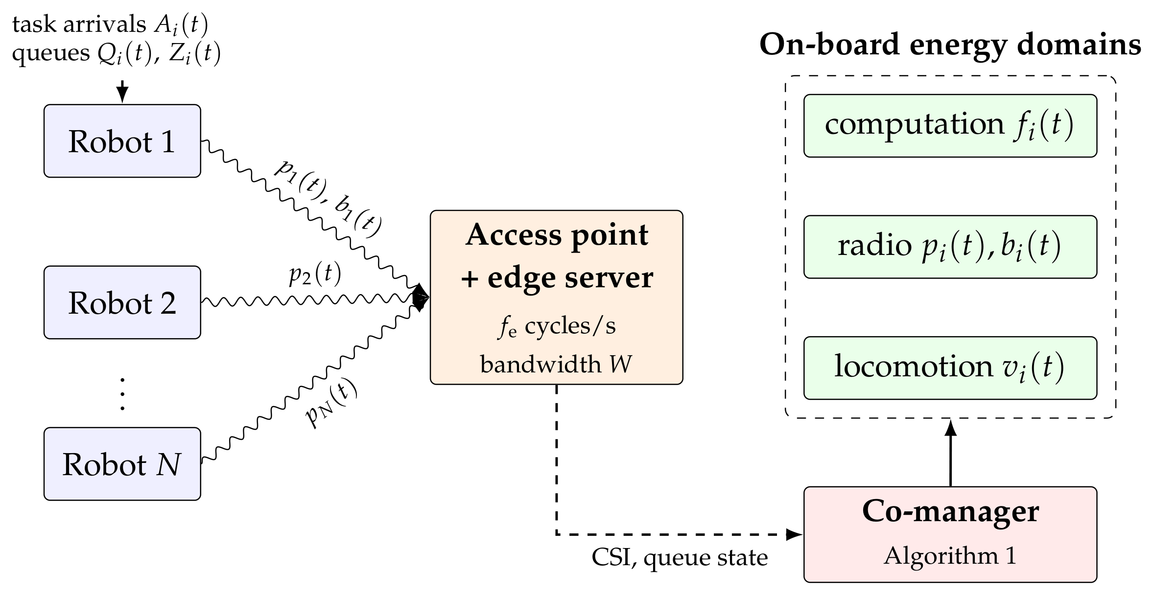
beyond which no channel condition can hold the robot back; with the parameters of Section 6 this is a debt of a few metres: a handful of seconds of travel. The second mechanism applies when the mission carries a hard temporal structure, a docking slot, a rendezvous, and a delivery window. Such a deadline has exactly the form of a task deadline and allows the treatment of Section 5.6: a feasibility floor $v_i^{\mathrm{dl}}\left(t\right)=$ (distance remaining)/(time remaining), clipped to $\mathcal{V}$ and applied as $v_i\left(t\right)=max\{v_i^{\star }\left(t\right),v_i^{\mathrm{dl}}\left(t\right)\}$. Under this floor the communication term can only exploit slack the mission has genuinely left unused, and a robot behind schedule stops trading motion for channel quality altogether. The evaluation did not need the floor with waypoint tours and hard arrival times (13), as these were never approached, but it is what we would recommend wherever mission timing is contractual rather than best-effort.

Table 2. Notation.

Symbol	Units	Meaning
$N,\tau ,t$	–, s, –	number of robots, slot duration, slot index
$A_i\left(t\right)$	bit	sensor data generated by robot i in slot t
L	cycle/bit	computational intensity of the processing pipeline
${\theta }_i\left(t\right)$	–	fraction of the arrival routed to the edge server
$Q_i\left(t\right),Z_i\left(t\right)$	bit	computation and transmission queue backlogs
$G_i\left(t\right)$	m	mission-progress virtual queue (distance debt)
$f_i\left(t\right)$	Hz	processor clock frequency
$\kappa ,P^{\mathrm{sta}}$	–, W	effective switched capacitance, static compute power
$p_i\left(t\right),b_i\left(t\right)$	W, –	transmit power, fraction of bandwidth
$W,N_0$	Hz, W/Hz	system bandwidth, noise PSD incl. noise figure
$h_i\left(t\right)$	–	channel power gain, Equation (7)
$\eta ,P^{\mathrm{ckt}}$	–, W	amplifier efficiency, RF circuit power
$v_i\left(t\right),\mathcal{V}$	m/s	speed and its admissible set
${\beta }_0,{\beta }_1,{\beta }_2$	W, W s/m, W s2/m2	locomotion power coefficients
$v^{\mathrm{nom}}$	m/s	nominal mission speed, Equation (12)
V	–	Lyapunov weight trading energy against delay
$\mu$	–	weight of the mission-progress virtual queue
$D^{max}$	s	end-to-end task deadline

lists the notation and Figure 1 presents the Co-management architecture.

4. Problem Formulation

4.1. The Co-Management Problem

Collect the decisions of slot t in $\mathbf{\Theta }\left(t\right)={\{{\theta }_i\left(t\right),f_i\left(t\right),p_i\left(t\right),b_i\left(t\right),v_i\left(t\right)\}}_{i\in \mathcal{N}}$. The co-management problem is

$$\begin{array}{cc}\hfill \mathbf{\left(}\mathbf{P}\mathbf{1}\mathbf{\right)}\underset{\{\mathbf{\Theta }(t\left)\right\}}{min}& \overline{E}:=\underset{T\to \infty }{lim\; sup}{\displaystyle \frac{1}{T}}{\displaystyle \sum _{t=0}^{T-1}}\sum _{i\in \mathcal{N}}\mathbb{E}\left[E_i\left(t\right)\right]\hfill \end{array}$$

(14a)

$$\begin{array}{cc}\hfill \mathrm{s}.\mathrm{t}.& Q_i\mathrm{and}{Z}_i\mathrm{are}\mathrm{mean}\text{-}\mathrm{rate}\mathrm{stable},\forall i,\hfill \end{array}$$

(14b)

$$\begin{array}{cc}\hfill & \underset{J\to \infty }{\mathrm{lim\; sup}}\frac{1}{J}{\sum }_{j=1}^{J}Pr\left[D_{ij}>D^{max}\right]\le {\epsilon }_{\mathrm{d}},\forall i,\hfill \end{array}$$

(14c)

$$\begin{array}{cc}\hfill & \underset{T\to \infty }{\lim }\frac{1}{T}{\sum }_t\mathbb{E}\left[v_i\left(t\right)\right]\ge v^{\mathrm{nom}},\forall i,\hfill \end{array}$$

(14d)

$$\begin{array}{cc}\hfill & {\sum }_{i\in \mathcal{N}}{b}_i\left(t\right)\le 1,b_i\left(t\right)\ge 0,\forall t,\hfill \end{array}$$

(14e)

$$\begin{array}{cc}\hfill & 0\le p_i\left(t\right)\le p^{max},f_i\left(t\right)\in \left\{0\right\}\cup [f^{min},f^{max}],\forall i,t,\hfill \end{array}$$

(14f)

$$\begin{array}{cc}\hfill & {\theta }_i\left(t\right)\in [0,1],v_i\left(t\right)\in \mathcal{V},\forall i,t.\hfill \end{array}$$

(14g)

Constraint (14c) states the deadline requirement explicitly, as a bound ${\epsilon }_{\mathrm{d}}$ on the long-run fraction of tasks whose end-to-end latency (3) exceeds $D^{max}$. It is worth being precise about why it has to appear separately rather than being inherited from the stability constraint (14b). Mean-rate stability bounds the time-average backlog, and Little’s law converts that into an average sojourn time; neither says anything about the tail. A policy can hold the mean backlog low while starving individual tasks indefinitely, and in fact, the drift-plus-penalty rules of Section 5 do exactly that if left unguarded: because the routing rule sends work to whichever queue is shorter and the clock rule serves a short queue slowly, a task can sit in the local queue for tens of seconds while the average backlog looks healthy. We observed precisely this failure in an earlier version of this work. Section 5.6 therefore adds an explicit per-task mechanism, and Section 6 reports measured per-task violation rates rather than a backlog-derived proxy.

4.2. Why (P1) Is Hard

Three separate difficulties compound here.

The problem is stochastic and non-anticipative. The arrivals $A_i\left(t\right)$ and the fading ${\varsigma }_i\left(t\right)$ are revealed slot by slot, and the objective is a long-run average, so an offline optimum would require the entire realisation in advance. Dynamic programming over the joint state, queue backlogs, positions, and channel gains for N robots is hopeless for any realistic N.

The per-slot problem is non-convex and mixed-integer. The speed $v_i\left(t\right)$ lives in a discrete set; the transmit energy (9) is discontinuous at the origin; and the objective couples continuous variables through the rate expression.

Finally, and most awkwardly, the decisions are coupled across time through the physical state. Choosing $v_i\left(t\right)$ changes ${\mathbf{x}}_i(t+1)$, which changes $h_i(t+1)$ through the shadowing field, which changes the cost of every subsequent transmission. Unlike the queue coupling, which the Lyapunov method handles cleanly, this is a coupling through a continuous exogenous field that the robot samples as it moves.

We deal with the first two exactly, in the sense that the algorithm of Section 5 comes with a provable bound, and with the third approximately, by a finite lookahead.

4.3. Virtual Queues

Constraint (14d) is a time-average inequality, not a per-slot one, so we convert it into a queue. Define the mission-progress queue

$$G_i(t+1)={[G_i\left(t\right)+\left(v^{\mathrm{nom}}-v_i\left(t\right)\right)\tau ]}^{+},$$

(15)

which accumulates, in metres, the distance the robot owes relative to driving at $v^{\mathrm{nom}}$ throughout. A standard argument shows that mean-rate stability of $G_i$ is equivalent to satisfaction of (14d) [41]. The robot may therefore fall behind temporarily, pausing to exploit a good link, but the growing debt increases the pressure to speed up, and the constraint is met in the limit.

Writing $\mathbf{\Theta }\left(t\right)=\left(\mathbf{Q}\right(t),\mathbf{Z}(t),\mathbf{G}(t\left)\right)$ for the full queue state, we take the quadratic Lyapunov function

$$\mathcal{L}\left(\mathbf{\Theta }\left(t\right)\right)={\displaystyle \frac{1}{2}}\sum _{i\in \mathcal{N}}\left(Q_i{\left(t\right)}^2+Z_i{\left(t\right)}^2+\mu G_i{\left(t\right)}^2\right),$$

(16)

where $\mu >0$ reconciles the units of the progress queue (metres) with those of the data queues (bits). The one-slot conditional drift is $\Delta (\mathbf{\Theta }(t\left)\right)=\mathbb{E}\left[\mathcal{L}\right(\mathbf{\Theta }(t+1))-\mathcal{L}(\mathbf{\Theta }\left(t\right))\mid \mathbf{\Theta }(t\left)\right]$.

5. The Co-Management Algorithm

5.1. Drift-Plus-Penalty Bound

Squaring (1), (2) and (15), using ${\left({\left[x\right]}^{+}\right)}^2\le x^2$ and the boundedness of arrivals and service rates, and collecting the constant terms into

$$B={\displaystyle \frac{1}{2}}\sum _{i\in \mathcal{N}}\left({\left(A^{max}\right)}^2+{\left(D^{\mathrm{c},\max }\right)}^2+{\left(D^{\mathrm{o},\max }\right)}^2+\mu {\tau }^2{\left(v^{\mathrm{nom}}\right)}^2+\mu {\tau }^2{v}_{max}^2\right),$$

(17)

we obtain the standard drift-plus-penalty inequality: for any $V>0$,

$$\begin{array}{cc}\hfill & \Delta \left(\mathbf{\Theta }\left(t\right)\right)+V\mathbb{E}\left[{\sum }_i{E}_i\left(t\right)|\mathbf{\Theta }\left(t\right)\right]\le B\hfill \\ \hfill & +\mathbb{E}\left[{\sum }_{i}V{E}_i\left(t\right)-Q_i\left(t\right)D_i^{\mathrm{c}}\left(t\right)-Z_i\left(t\right)D_i^{\mathrm{o}}\left(t\right)|\mathbf{\Theta }\left(t\right)\right]\hfill \\ \hfill & +\mathbb{E}\left[{\sum }_i{Q}_i\left(t\right)\left(1-{\theta }_i\left(t\right)\right)A_i\left(t\right)+Z_i\left(t\right){\theta }_i\left(t\right)A_i\left(t\right)|\mathbf{\Theta }\left(t\right)\right]\hfill \\ \hfill & +\mathbb{E}\left[{\sum }_i\mu G_i\left(t\right)\left(v^{\mathrm{nom}}-v_i\left(t\right)\right)\tau |\mathbf{\Theta }\left(t\right)\right].\hfill \end{array}$$

(18)

The algorithm is the usual opportunistic one: observe $\mathbf{\Theta }\left(t\right)$, the arrivals and the channel gains, and choose the decisions that minimise the right-hand side of (18) in this slot. Because no expectation is needed to do that, the policy requires no statistics of $A_i$ or $h_i$.

What makes the resulting problem tractable is that the right-hand side separates. The terms involving $f_i$, those involving $(p_i,b_i)$, those involving ${\theta }_i$ and those involving $v_i$ do not interact within a slot except through the shared bandwidth constraint (14e), which couples the $b_i$ across robots but nothing else. We therefore solve four subproblems.

5.2. Subproblem 1: Processor Clock

Dropping terms that do not involve $f_i$ and substituting (4) and (5), the frequency in slot t solves

$$\underset{f_i\in \left\{0\right\}\cup [f^{min},f^{max}]}{min}V\left(\kappa f_i^3+P^{\mathrm{sta}}\right)\tau -Q_i\left(t\right){\displaystyle \frac{f_i\tau }{L}}.$$

(19)

Proposition 1 (Square-root clock rule).

Assume $Q_i\left(t\right)\ge f^{max}\tau /L$, so the backlog is not exhausted within the slot. The minimiser of (19) over the continuous branch is

$$f_i^{\star }\left(t\right)=min\left\{f^{max},\sqrt{{\displaystyle \frac{Q_i\left(t\right)}{3V\kappa L}}}\right\},$$

(20)

and the processor should be gated off entirely, $f_i^{\star }\left(t\right)=0$, whenever the value of (19) at $f_i^{\star }$ exceeds zero.

Proof. 

The objective is strictly convex on $[f^{min},f^{max}]$ with derivative $3V\kappa f_i^2\tau -Q_i\tau /L$, which vanishes at $f_i=\sqrt{Q_i/\left(3V\kappa L\right)}$; clipping to the box gives (20). The isolated point $f_i=0$ has objective value 0 and must be compared separately, which yields the gating test. □

Proposition 1 is worth reading physically. The clock tracks the square root of the backlog, so the processor speeds up as work piles up but with strongly diminishing aggression, exactly the behaviour one wants given that power grows cubically. The clock also falls as $V^{-1/2}$: a deployment that cares more about energy than latency runs its processor slower and lets queues grow, which is the energy–delay tradeoff appearing in a single scalar.

5.3. Subproblem 2: Transmit Power and Bandwidth

The radio terms give

$$\underset{\{p_i,b_i\}}{min}\sum _{i\in \mathcal{N}}\left[V\left({\displaystyle \frac{p_i}{\eta }}+P^{\mathrm{ckt}}\right)\tau -Z_i\left(t\right)b_{i}W{log}_2\left(1+{\displaystyle \frac{p_i{h}_i\left(t\right)}{b_{i}W{N}_0}}\right)\tau \right]\mathrm{s}.\mathrm{t}.\sum _i{b}_i\le 1,$$

(21)

subject to $0\le p_i\le p^{max}$.

Lemma 1.

The function $(p,b)\mapsto bW{log}_2\left(1+ph/\left(bW{N}_0\right)\right)$ is jointly concave on $\{p\ge 0,b>0\}$.

Proof. 

It is the perspective $b\varphi (p/b)$ of the concave function $\varphi \left(u\right)=W{log}_2(1+uh/\left(W{N}_0\right))$, and the perspective operation preserves concavity ([42] Section 3.2.6). □

Hence (21) is a convex program on the continuous branch and can be solved by partial dualisation of the bandwidth constraint. Attaching a multiplier $\nu \ge 0$ to ${\sum }_i{b}_i\le 1$ decouples the robots, and for a fixed $b_i$ the inner minimisation over $p_i$ has a closed form.

Proposition 2 (Guarded water-filling).

For fixed $b_i>0$, the minimiser of (21) over $p_i\in [0,p^{max}]$ on the active branch is

$${\tilde{p}}_i\left(t\right)=min\left\{p^{max},{\left[b_{i}W\left({\displaystyle \frac{Z_i\left(t\right)\eta }{Vln2}}-{\displaystyle \frac{N_0}{h_i\left(t\right)}}\right)\right]}^{+}\right\},$$

(22)

and the transmitter is activated only if doing so is worthwhile,

$$p_i^{\star }\left(t\right)={\tilde{p}}_i\left(t\right)\mathrm{if}V({\tilde{p}}_i/\eta +P^{\mathrm{ckt}})\tau <Z_i\left(t\right){\tilde{r}}_i\tau ,p_i^{\star }\left(t\right)=0otherwise,$$

(23)

where ${\tilde{r}}_i$ is the rate (8) evaluated at ${\tilde{p}}_i$.

Proof. 

Setting the derivative of the i-th summand of (21) with respect to $p_i$ to zero gives $V/\eta =Z_i{h}_i/\left(N_{0}ln2(1+p_i{h}_i/\left(b_{i}W{N}_0\right))\right)$, which rearranges to (22); convexity makes the stationary point the minimiser, and clipping handles the box. The circuit term makes the objective discontinuous at $p_i=0$, so the value at the origin must be compared explicitly, giving (23). □

Equation (22) is a water-filling rule in which the water level $Z_i\eta /(Vln2)$ is set by the transmit backlog rather than by a power budget: a robot with a lot of queued data raises its level and tolerates a worse channel, while a robot with little to send transmits only when $h_i>V{N}_{0}ln2/\left(Z_i\eta \right)$. The guard (23) is what keeps the radio from dribbling. Together they produce the qualitative behaviour that motivated the paper, a robot in a shadowed spot with a modest backlog simply waits.

Caution is required before dualising the bandwidth constraint. The per-robot objective is convex only on the active branch $p_i>0$; the fixed activation cost $P^{\mathrm{ckt}}$ makes the full objective, with the on/off decision included, non-convex, and strong duality cannot be invoked for it. What can be said is the following. For a fixed on/off pattern the problem is convex by Lemma 1, the dual function (a pointwise minimum of affine functions of $\nu$) is concave, and bisection on $\nu$ recovers the $ϵ$-optimal allocation for that pattern in $O(log(1/ϵ\left)\right)$ iterations [43]; the on/off pattern itself is then resolved per robot by the explicit comparison (23) at the recovered allocation. The composition is a coordinate-style heuristic for the mixed problem, not a global optimum, and a duality gap of at most $NV{P}^{\mathrm{ckt}}\tau$ the total activation cost that the relaxation can misattribute separates it from the true minimum. Since the per-slot problem is itself only one term of an infinite-horizon bound, we regard the gap as one more additive constant absorbed into B, and we verify in Section 6 that the implemented allocator does minimise the per-slot objective it is asked to minimise. The implementation used throughout Section 6 is this bisection, so the evaluated policy is the policy analysed here; the equal-share allocation appears only as an ablation variant, where interestingly it performs slightly better in closed loop, a point Section 6.8 returns to.

5.4. Subproblem 3: Offloading Split

The arrival terms in (18) involving ${\theta }_i$ are $Q_i\left(t\right)(1-{\theta }_i)A_i\left(t\right)+Z_i\left(t\right){\theta }_i{A}_i\left(t\right)$, linear in ${\theta }_i$; taken alone they yield a pure join-the-shorter-queue rule, ${\theta }_i=1$ iff $Z_i\left(t\right)\le Q_i\left(t\right)$. An earlier version of this work used exactly that rule, and it is instructive to record why it is insufficient. Join-the-shorter-queue is the drift minimiser only when the marginal cost of serving a bit is the same in both pipes; here it is not. A bit served locally costs $(P^{\mathrm{c}}\left(f\right)-P^{\mathrm{idle}})L/f$ joules while a bit transmitted costs $(p/\eta +P^{\mathrm{ckt}}-P^{\mathrm{rx}})/r$ joules, and the two differ by an order of magnitude depending on the channel. Since the routing decision also determines which pipe’s energy term in (18) the arrival will eventually activate, the correct per-slot comparison includes both the queue pressure and V times the marginal energy of the destination pipe:

$${\theta }_i^{\star }\left(t\right)=\left\{\begin{array}{cc}1,\hfill & V{e}_i^{\mathrm{o}}\left(t\right)+Z_i\left(t\right)\le V{e}_i^{\mathrm{c}}\left(t\right)+Q_i\left(t\right),\hfill \\ 0,\hfill & \mathrm{otherwise},\hfill \end{array}\right.$$

(24)

where $e_i^{\mathrm{c}}\left(t\right)$ and $e_i^{\mathrm{o}}\left(t\right)$ are the current marginal energies per bit of the local and offload paths, evaluated at the operating points of subproblems 1 and 2. The rule additionally vetoes the offload path for a task whose transmission, server execution and return could not complete within $D^{max}$ even if started immediately; Section 5.6 develops this. The rule is bang-bang, which raises the question of chattering when the two sides of (24) are nearly equal and the backlogs fluctuate rapidly. Two standard softenings are available and both preserve the drift bound: a hysteresis dead-band, in which the previously selected pipe is retained unless the alternative is better by a margin ${\varrho }_{\mathrm{h}}max\left\{\right|J_i^{\mathrm{c}}|,|J_i^{\mathrm{o}}\left|\right\}$, and threshold randomisation, in which the two pipes are chosen with probabilities interpolating linearly across a dead-band of the same width, so that a fractional split is realised in expectation. Because both agree with (24) outside the band and the band can be made arbitrarily narrow, the added drift is bounded by ${\varrho }_{\mathrm{h}}{A}^{max}{max}_i\{Q_i,Z_i\}$ per slot and vanishes with ${\varrho }_{\mathrm{h}}$. We evaluate both in Section 6.10; the short answer is that they are harmless but, in this system, unnecessary; the queue-time-scale separation between the slot and the backlog dynamics means the raw rule does not in fact chatter enough to matter.

5.5. Subproblem 4: Speed Selection

The remaining terms give the locomotion subproblem. A robot’s speed affects the drift in two ways: directly through the progress queue, and indirectly through the channel it will experience over the coming slots. We capture the latter with a finite lookahead of H slots along the current heading:

$$v_i^{\star }\left(t\right)=\underset{v\in \mathcal{V}}{arg\; min}\left\{V{P}^{\mathrm{v}}\left(v\right)\tau +\mu G_i\left(t\right)\left(v^{\mathrm{nom}}-v\right)\tau -Z_i\left(t\right){\overline{r}}_i\left(v\right)\tau \right\},$$

(25)

where

$${\overline{r}}_i\left(v\right)={\displaystyle \frac{1}{H}}{\displaystyle \sum _{k=1}^H}r\left(p_i^{\star }\left(t\right),b_i\left(t\right),\overline{h}\left({\mathbf{x}}_i\left(t\right)+kv\tau {\mathbf{u}}_i\left(t\right)\right)\right)$$

(26)

is the mean rate predicted along the heading ${\mathbf{u}}_i\left(t\right)$, evaluated using the large-scale gain $\overline{h}$ only; that is, path loss and the shadowing field, with the fading averaged out. Obtaining $\overline{h}$ requires a coverage map of the workspace, which in practice is either built during a commissioning pass or accumulated online from the robots’ own RSSI reports; this is routine in industrial deployments and we treat the map as given.

The three terms of (25) say something quite intuitive. The first prices the locomotion energy. The second is the pressure from accumulated distance debt, which grows whenever the robot lingers and eventually forces it to move. The third is the value of the data it could push through the link along each candidate path, weighted by how much data is waiting. A robot with an empty transmit queue ignores the third term and simply drives; one holding a large backlog will decline to drive into a shadowing dip until it has cleared enough of it, then make the distance up later.

Since $\left|\mathcal{V}\right|$ is small, six set-points in our experiments, the minimisation is a direct enumeration, and the lookahead (26) needs only a handful of samples of the coverage map.

5.6. Per-Task Deadline Enforcement

The rules derived so far stabilise the queues and control the average backlog, but constraint (14c) is a statement about individual tasks, and drift arguments do not deliver it. Worse, the rules can actively work against it: the routing rule diverts arrivals away from a congested pipe, the clock rule serves a short queue slowly, and the combination can strand a handful of tasks in a nearly-empty local queue for tens of seconds while every time-average looks healthy. We observed exactly this pathology, individual sojourn times close to 80 $\mathrm{s}$ against a mean of 170 $\mathrm{m}$$\mathrm{s}$ before adding the mechanism of this subsection.

The mechanism is a pair of feasibility floors, evaluated per-slot from the FIFO order of the queues. For the local queue, the smallest clock that keeps every queued task feasible is

$$f_i^{\mathrm{dl}}\left(t\right)=min\left\{f^{max},\underset{j\in {\mathcal{Q}}_i\left(t\right)}{max}{\displaystyle \frac{L{\sum }_{k⪯j}{a}_k\left(t\right)}{{[D^{max}-(t-t_j^{\mathrm{arr}})-\tau ]}^{+}}}\right\},$$

(27)

where $a_k\left(t\right)$ are the residual bits of the tasks at or ahead of position j, and the clock actually applied is $max\{f_i^{\star }\left(t\right),f_i^{\mathrm{dl}}\left(t\right)\}$ with $f_i^{\star }$ from Proposition 1. For the transmit queue, the guard of Proposition 2 is overridden, and the radio transmits at $p^{max}$ whenever the head-of-line task’s remaining slack, the net of a reserve for server execution and the return link, falls below two slots. The routing veto in (24) plays the complementary preventive role.

Two remarks. First, the floors are exact for the local path, whose service rate is deterministic given f, but necessarily approximate for the offload path, whose transmission time depends on the fading; the reserve absorbs the typical error and the residual appears as the small measured violation rates of Section 6. Second, the floors interact with the energy–delay tradeoff in a way the unconstrained theory does not predict: beyond a critical V the square-root rule alone would let queues grow, the floor (27) engages more and more often, and total energy rises with V instead of falling. The unconstrained $\left[O\right(1/V),O(V\left)\right]$ curve is therefore truncated in practice at the V where the deadline mechanism becomes the binding control, and the useful operating range is below it.

5.7. Algorithm Summary and Complexity

Algorithm 1 collects the four rules. Its per-slot cost is $O\left(N(log(1/ϵ)+H|\mathcal{V}\left|\right)\right)$: the bandwidth bisection contributes the logarithmic term, the speed lookahead the second, and the clock, power and routing rules are $O\left(1\right)$ each. With $N=8$, $H=40$ and $\left|\mathcal{V}\right|=6$ the whole update is a few hundred floating-point operations, which is negligible next to the perception workload it is scheduling. The per-robot rules depend only on that robot’s own state, so lines 7–14 run independently on each platform; only the bandwidth allocation is centralised, and even that can be dispensed with at a small loss.

Memory is $O\left(N\right)$ plus the coverage map. No model of the arrival process, the fading distribution or the mobility pattern is required at any point.

5.8. Performance Guarantee

Let ${\overline{E}}^{\star }$ denote the optimal value of (14) over all policies, including those with complete knowledge of the arrival and channel statistics.

Theorem 1 (Energy-delay tradeoff).

Suppose the arrival and channel processes are i.i.d. across slots and that there exists a policy satisfying (14b)–(14g) with slack $ϵ>0$. Then under Algorithm 1, for every $V>0$:

$$\begin{array}{cc}\hfill \underset{T\to \infty }{lim\; sup}{\displaystyle \frac{1}{T}}{\displaystyle \sum _{t=0}^{T-1}}\sum _i\mathbb{E}\left[E_i\left(t\right)\right]& \le {\overline{E}}^{\star }+{\displaystyle \frac{B}{V}},\hfill \end{array}$$

(28)

$$\begin{array}{cc}\hfill \underset{T\to \infty }{lim\; sup}{\displaystyle \frac{1}{T}}{\displaystyle \sum _{t=0}^{T-1}}\sum _i\mathbb{E}\left[Q_i\left(t\right)+Z_i\left(t\right)+\mu G_i\left(t\right)\right]& \le {\displaystyle \frac{B+V\left({\overline{E}}^{\star }-E^{min}\right)}{ϵ}},\hfill \end{array}$$

(29)

with B as in (17) and $E^{min}$ a lower bound on the per-slot energy. All queues are mean-rate stable, so constraint (14d) holds.

The proof is the standard drift-plus-penalty argument applied to (18); we give it in Appendix A for completeness. The content of Theorem 1 is the familiar $\left[O\right(1/V),O(V\left)\right]$ pair: the energy gap closes as V grows, at the price of backlogs, and hence delay, that grow proportionally. In practice V is chosen as large as the deadline budget permits, and Section 6 traces the curve.

Three qualifications keep the theorem from claiming more than it delivers. (i) Controlled channel. $h_i\left(t\right)$ depends on ${\mathbf{x}}_i\left(t\right)$, which the speed rule itself steers, so the classical exogenous-state assumption holds only for a fixed speed profile (the baselines’ regime). What survives regardless is stability: (29) holds for every realisation because it descends from a per-slot comparison; the near-optimality gap $B/V$ in (28), however, is then relative to the best policy within the same speed profile rather than to a globally optimal one. (ii) Lookahead penalty. The speed rule uses a predicted rate ${\overline{r}}_i\left(v\right)$; a bounded prediction error $|{\overline{r}}_i\left(v\right)-\mathbb{E}[r_i\mid v]|\le {\Delta }_r$ adds $\overline{Z}{\Delta }_r\tau /V=O\left({\Delta }_r\right)$ to (28), vanishing with the map error, which the sensitivity study of Section 6 confirms is small in practice. (iii) Deadline floors sit outside the theorem. The floors of Section 5.6 override the drift-minimising decisions when a deadline is at risk; the bound absorbs this as an additive term proportional to how often that happens, and is silent once the floors engage persistently, exactly the regime in which Section 6 observes energy rising with V beyond a knee.

6. Evaluation

6.1. Setup

We evaluate Algorithm 1 in a discrete-event simulation of the model of Section 3, with every task tracked individually through the pipeline of (3): queueing, local execution or transmission, edge-server queueing and execution, and the return link. The edge server is a shared FIFO resource of rate f_e = 20 Gcycle s⁻¹ serving the whole fleet, and results of size $\varrho =0.05$ of the task return over a 50 Mbit s⁻¹ downlink. Robots follow independent random waypoint tours: each robot drives to a sequence of uniformly drawn waypoints, and waypoints completed is the measure of mission progress, so all policies are compared at equal work accomplished rather than merely at equal average speed. The shadowing field, waypoint sequences and arrival processes are redrawn per seed.

Table 3. Simulation parameters (version 2).

Parameter	Value	Comment
Slot $\tau$; workspace	100 $\mathrm{m}$$\mathrm{s}$; 160 $\mathrm{m}$ sq.	AP at centre
Robots N; bandwidth W	8 (2–16 in scaling); 20 $\mathrm{M}$$\mathrm{Hz}$	OFDMA
Noise PSD; $g_0$; $\alpha$	−174 dB mHz−1 + 8 dB; −45 dB; 4.0	indoor/industrial
Shadowing ${\sigma }_{\mathrm{sh}}$; decorr.	6 dB; 8 m	correlated field
$p^{max}$; $\eta$; $P^{\mathrm{ckt}}$; $P^{\mathrm{rx}}$	0.5 W; 0.35; 0.10 W; 0.05W	gated radio model
$[f^{min},f^{max}]$; $\kappa$	$[0.2,2.4]$ $\mathrm{G}\mathrm{Hz}$; ${10}^{-27}$	DVFS
$P^{\mathrm{act}}$; $P^{\mathrm{idle}}$	0.55 $\mathrm{W}$; 0.18 $\mathrm{W}$	gated compute model
Intensity L; deadline $D^{max}$	200 cycle bit−1; 500 ms
Edge $f_{\mathrm{e}}$; downlink; $\varrho$	20 Gcycle s−1; 50 Mbit s−1; 0.05	shared FIFO server
$({\beta }_0,{\beta }_1,{\beta }_2)$; $\mathcal{V}$; $v^{\mathrm{nom}}$	$(1.9,2.4,1.1)$; $\{0,\dots ,1.5\}$ $\mathrm{m} {\mathrm{s}}^{-1}$; $0.9$$\mathrm{m} {\mathrm{s}}^{-1}$	waypoint tours
Load $\lambda$; V; $\mu$; H	0.8 $\mathrm{M}$$\mathrm{bit}$/slot; ${10}^{12}$; $2\times {10}^{12}$; 40	defaults
Seeds; slots	10 × 2500 (headline); 4–5 × 1200 (sweeps)	400/250-slot warm-up

lists the parameters; they are representative of a mid-range industrial AMR and are illustrative rather than measured from a specific product.

Each reported point is the mean over independent seeded runs, ten seeds of 2500 slots (250 s) for the headline comparison, with a 40 s warm-up excluded, and four to five seeds of 1200 slots for the parameter sweeps. Intervals shown are 95% bootstrap confidence intervals over seeds, and the headline energy comparison additionally reports a Welch two-sample test. Latency percentiles are computed over completed tasks; any task still unfinished at the end of a run is counted as a deadline violation, so the violation figures cannot be flattered by stranding work.

6.2. Baselines

Seven schemes are compared. Local-only processes everything on board at $f^{max}$. Full-offload sends everything to the edge at $p^{max}$. Decoupled alternates the offloading split evenly and optimises neither jointly. Myopic greedy picks, per task, whichever pipe is cheaper for that task in isolation and serves it at the minimum sufficient rate. Two stronger baselines respond to the criticism that a fixed-split decoupled design is easy to beat: MEC-opt offloads on a channel-quality threshold, runs DVFS locally, and represents a well-engineered mobility-oblivious MEC design; mobility-aware additionally offloads when the robot is closing on the access point, representing the heading-conditioned heuristics of the cloud-robotics literature. All baselines drive at $v^{\mathrm{nom}}$ and complete the same waypoint tours as the proposed scheme to within 2%.

6.3. Headline Comparison

Table 4. Performance at the default operating point ($N=8$, $\lambda =0.8 \mathrm{M}\mathrm{bit}$ per slot, $V={10}^{12}$, ten seeds). ICT is communication plus computation power. Brackets are 95% bootstrap confidence intervals on total power. Violations are per completed task, with unfinished tasks counted as violations. Schemes marked † violate the deadline constraint (14c) and are not valid operating points.

Scheme	Total ($\mathbf{W}$)	ICT ($\mathbf{W}$)	Mean Lat. ($\mathbf{m}\mathbf{s}$)	p95 ($\mathbf{m}\mathbf{s}$)	Viol. (%)	WP/min
Local-only	17.43 [17.41, 17.44]	11.53	66.8	94.3	0.00	0.87
Full-offload †	7.23 [7.18, 7.29]	1.34	1754.3	10,690.0	19.50	0.87
Decoupled	12.38 [12.34, 12.43]	6.49	189.8	250.0	2.00	0.87
Myopic greedy †	7.40 [7.31, 7.51]	1.51	442.1	2540.0	10.02	0.87
MEC-opt	8.26 [8.02, 8.55]	2.37	105.7	200.0	0.00	0.87
Mobility-aware †	7.63 [7.49, 7.79]	1.74	747.0	4240.0	10.28	0.87
Proposed	7.65 [7.59, 7.71]	1.78	133.9	240.1	0.16	0.86

reports the default operating point. The picture is sharper, and more modest, than the one an earlier version of this manuscript painted with a backlog-derived delay proxy, and it is worth being explicit about both.

First the sanity check that the per-task accounting restores: local-only now shows a mean latency of $66.8$ $\mathrm{m}$$\mathrm{s}$, which is what arithmetic requires, since a $0.8$ $\mathrm{M}$$\mathrm{bit}$ task at 200 $\mathrm{cycle}$ ${\mathrm{bit}}^{-1}$ on a $2.4$ $\mathrm{G}$$\mathrm{Hz}$ core needs $66.7$ $\mathrm{m}$$\mathrm{s}$ of execution alone.

Second the honest headline. Three schemes achieve lower total energy than the proposed policy: full-offload, myopic greedy and mobility-aware. All three buy it by missing deadlines, 19.5%, 10.0% and 10.3% of tasks respectively and are therefore not valid operating points for a system with a 500 $\mathrm{m}$$\mathrm{s}$ control-loop budget. Among the schemes that meet the deadline, the strongest competitor is MEC-opt at $2.37$ $\mathrm{W}$ of combined communication and computation (ICT) power; the proposed policy draws $1.78$ $\mathrm{W}$, a saving of 24.8% (Welch $t=4.15$, $p=3.4\times {10}^{-5}$, $n=10$ seeds per arm), at comparable latency (134 $\mathrm{m}$$\mathrm{s}$ vs. 106 $\mathrm{m}$$\mathrm{s}$ mean, 240 vs. 200 $\mathrm{m}$$\mathrm{s}$ 95th percentile) and equal mission progress. Against the weak fixed-split decoupled baseline the saving is 72.5%, but we regard MEC-opt as the fair comparison and quote the smaller number as the contribution.

6.4. The Energy–Delay Tradeoff

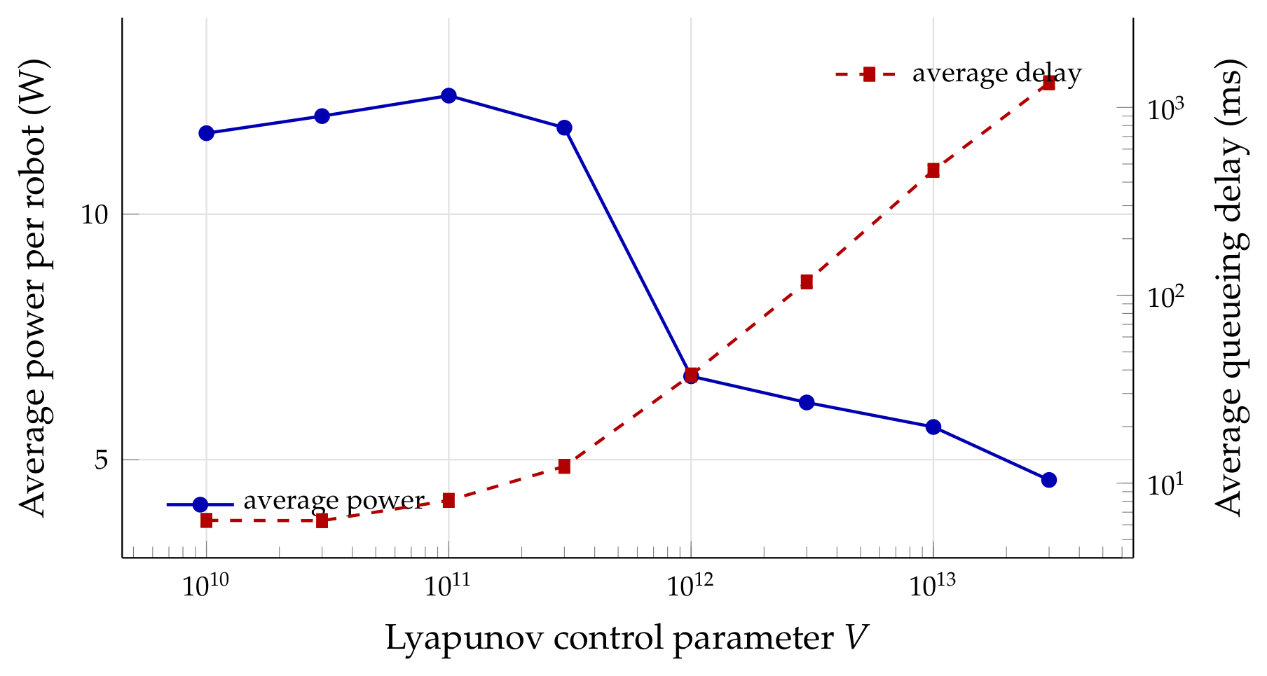
Figure 2 sweeps the Lyapunov weight over $V\in [3\times {10}^{10},{10}^{13}]$. Average power falls from $10.07$ to $6.98$ $\mathrm{W}$ and mean latency rises from 118 to 199 $\mathrm{m}$$\mathrm{s}$, the qualitative $\left[O\right(1/V),O(V\left)\right]$ shape of Theorem 1. Two departures from the unconstrained theory are visible and both are consequences of the deadline mechanism of Section 5.6. The latency curve saturates rather than growing linearly, because the floors cap individual sojourns; and the violation rate creeps up with V ($0.11$ to 1.84% across the sweep) as the floors are asked to intervene more often against an increasingly energy-hungry drift term. We adopt $V={10}^{12}$, before the violation creep becomes material.

6.5. Load and Deadline Compliance

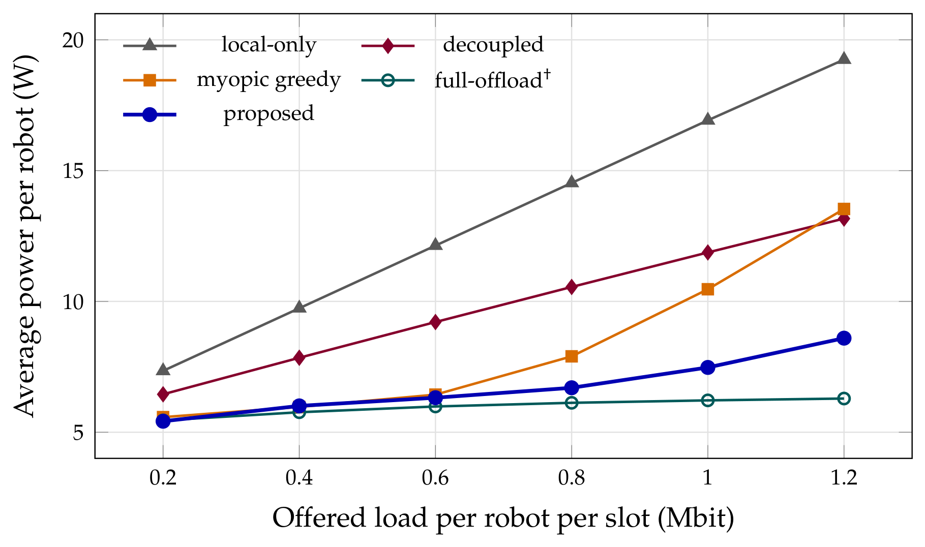
Figure 3 and Figure 4 sweep the offered load from 2 to 12 Mbit s⁻¹ per robot. On energy the proposed policy and the deadline-violating trio track each other within a few tenths of a watt across the range, the energy frontier is genuinely close to what full-offload achieves, while MEC-opt pays a growing premium for its channel-threshold conservatism, reaching $10.39$ $\mathrm{W}$ at the top of the range against $9.25$ $\mathrm{W}$ for the proposed policy.

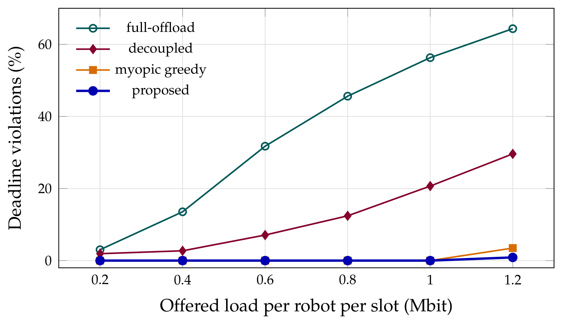
The separation is in Figure 4. At $1.2$ $\mathrm{M}$$\mathrm{bit}$ per slot the workload exceeds what several architectures can carry at all: local-only collapses to 46.9% violations (the load exceeds the on-board core’s capacity), greedy and mobility-aware to $54.9$ and 53.0%, and even MEC-opt reaches 16.5%. The proposed policy holds 0.42% across the entire range, the deadline floors, the routing veto and the adaptive split together keep the work flowing to whichever resource can still meet the budget. This robustness under load, rather than a large energy margin, is the operationally significant advantage.

6.6. Where the Energy Goes

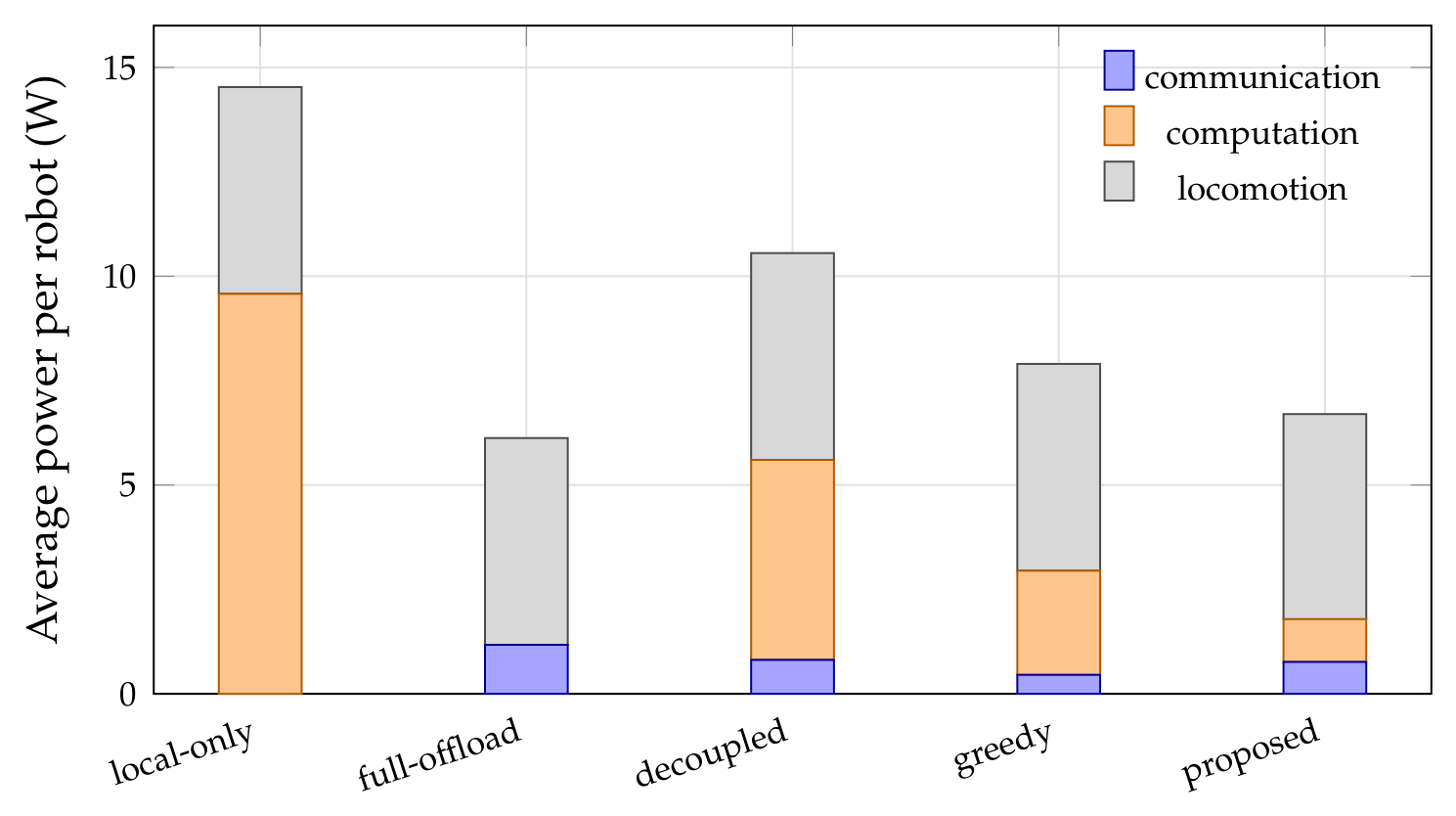
Figure 5 decomposes the default operating point. Locomotion ($5.89$ $\mathrm{W}$) is common to all schemes by construction. The proposed policy’s ICT split, $1.28$ $\mathrm{W}$ radio, $0.50$ $\mathrm{W}$ processor shows the same qualitative mechanism as before: relative to MEC-opt it spends 45% more on the radio to spend 66% less on the processor, because shipping a bit through a decent channel is cheaper than retiring its cycles locally, and the joint objective is what licenses making that exchange aggressively.

6.7. Scalability

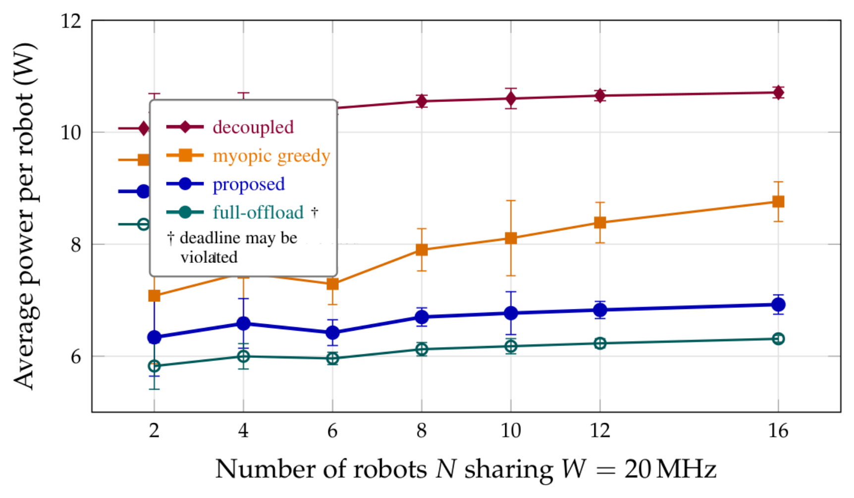
Figure 6 varies the fleet from 2 to 16 robots at fixed total bandwidth. The proposed policy is essentially flat ($8.14$ to $8.25$ $\mathrm{W}$) and, more tellingly, has three to eight times less seed-to-seed variance than the heuristic baselines at small N. Mobility awareness ranges from $\pm 1.05 \mathrm{W}$ at $N=2$ to $\pm 0.14 \mathrm{W}$ for the proposed policy because the queue-driven rules adapt to whatever channel geometry a seed produces instead of relying on thresholds tuned for the average one.

6.8. Ablation

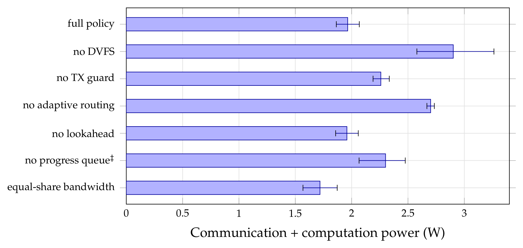
Figure 7 disables each mechanism in turn and reports ICT power with 95% confidence intervals; Table 3 conditions apply. Three mechanisms carry the design: removing DVFS raises ICT power from $1.97$ to $2.90$ $\mathrm{W}$ ($+47\%$), removing the adaptive routing to $2.70$ $\mathrm{W}$ ($+37\%$), and removing the transmit guard to $2.26$ $\mathrm{W}$ ($+15\%$). Removing the mission-progress queue produces the lowest total power of any variant and zero waypoints completed: the robots simply stop, which is precisely the confound the progress constraint exists to close, now demonstrated rather than asserted.

Two results are negative, and we report them as such. Disabling the channel lookahead changes nothing measurable ($1.96$ vs. $1.97$ $\mathrm{W}$, intervals overlapping almost entirely); we probed this under deeper shadowing, longer correlation lengths and deadlines relaxed to 4 $\mathrm{s}$, and the null persists. The structural reason is that the energy-aware router keeps the transmit queue small and the deadline reserve keeps it urgent, so the $Z_i{\overline{r}}_i\left(v\right)$ term in (25) is almost never large enough to override the progress pressure. The very mechanisms that fixed the deadline pathology removed the temporal slack that motion adaptation needs. In this scenario class the motion coupling is real in the model but contributes no measurable energy in the policy, and claims about it elsewhere in the paper are limited accordingly. Second, replacing the bandwidth bisection with an equal share lowers ICT power to $1.72$ $\mathrm{W}$. We verified that the bisection does minimise the per-slot objective it is derived from (it attains a strictly better drift-plus-penalty value and serves more bits per slot); the closed-loop reversal arises because draining transmit queues faster feeds back through the routing rule and pushes more traffic onto the radio. It is a concrete instance of the gap, flagged in Section 5, between per-slot drift minimisation and closed-loop optimality when the state is controlled.

6.9. Robustness to Bursty Arrivals and Correlated Fading

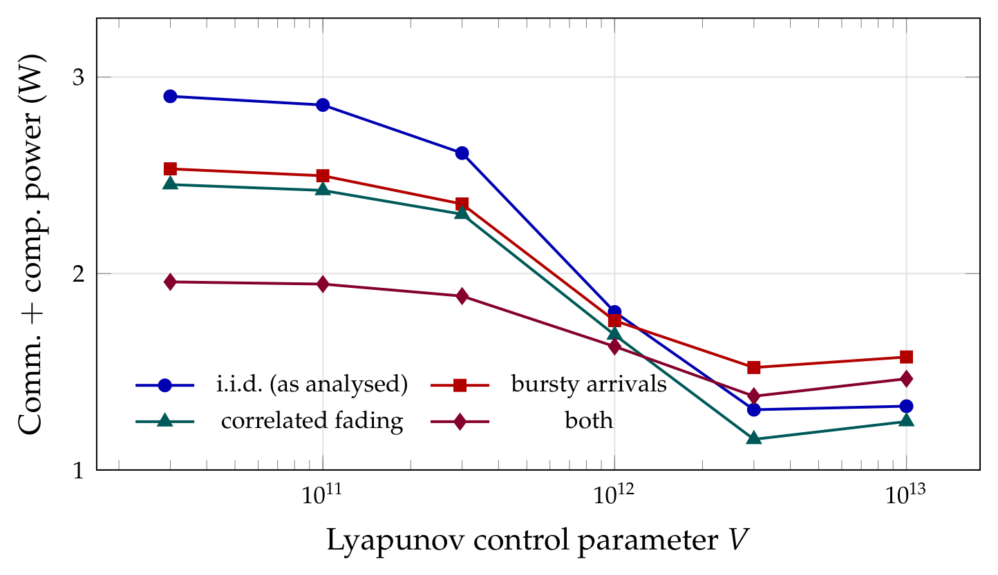
Theorem 1 assumes i.i.d. arrivals and channel states, and Section 5 already qualifies what that does and does not license. Since real robot workloads are bursty and real channels are correlated in time, the empirical question of whether the tradeoff survives qualitatively is worth answering directly. We therefore re-ran the V-sweep under three departures from the analysed statistics: arrivals generated by a two-state Markov-modulated ON/OFF source calibrated to the same mean, fading generated by a first-order Gauss–Markov process with one-slot correlation $\rho =0.95$, and both together.

Figure 8 shows the answer for energy. The monotone decrease of ICT power with V is preserved in every regime, and the curves are close: across the range the correlated-fading curve sits slightly below the i.i.d. one (correlation is exploitable, a good slot predicts another good slot, which the water-filling rule addresses), and the bursty curve is within $0.25$ $\mathrm{W}$ of it. The $\left[O\right(1/V),O(V\left)\right]$ shape is therefore qualitatively robust to both departures, which is a reassurance the analysis cannot supply.

The deadline picture is not robust, and we report it plainly. Under bursty arrivals the violation rate rises from below 0.1% to 8.7% at $V=3\times {10}^{10}$ and 10.5% at $V={10}^{13}$, essentially independent of V. The mechanism is transparent: the feasibility floors of Section 5.6 size the clock and the transmit power against the work already queued, so they react to a burst rather than anticipating it, and a burst arriving at several times the mean rate within one slot cannot be absorbed within the deadline no matter how the energy–delay knob is set. Correlated fading alone causes no such degradation. The practical implication is that the deadline machinery as formulated is adequate for smooth workloads and inadequate for bursty ones; an arrival-predictive floor, sizing the clock against a short-horizon forecast rather than the instantaneous backlog, is the natural remedy and we flag it in Section 7 as the most important open item.

6.10. Routing: Dead-Band and Randomisation

Table 5. Routing rule variants (four seeds, 1200 slots). ${\varrho }_{\mathrm{h}}$ is the dead-band width. Differences are within seed noise.

Variant	Regime	ICT ($\mathbf{W}$)	Mean Lat. (ms)	p95 (ms)	Viol. (%)
Bang-bang	steady	1.797	127.6	200	0.13
Hysteresis ${\varrho }_{\mathrm{h}}=0.10$	steady	1.794	127.3	200	0.15
Hysteresis ${\varrho }_{\mathrm{h}}=0.20$	steady	1.792	127.0	200	0.15
Hysteresis ${\varrho }_{\mathrm{h}}=0.40$	steady	1.795	126.6	200	0.18
Randomised ${\varrho }_{\mathrm{h}}=0.20$	steady	1.796	129.6	200	0.12
Bang-bang	bursty	1.777	237.4	700	9.11
Hysteresis ${\varrho }_{\mathrm{h}}=0.20$	bursty	1.772	236.5	700	9.03
Hysteresis ${\varrho }_{\mathrm{h}}=0.40$	bursty	1.757	236.2	700	9.05

compares the bang-bang rule of (24) with the hysteresis and randomisation variants of Section 5 at three dead-band widths and in both the steady and bursty regimes. All differences are within seed noise (ICT power moves by less than $0.021$ $\mathrm{W}$ across ${\varrho }_{\mathrm{h}}\in \{0.1,0.2,0.4\}$; violation rates are indistinguishable). Chattering is not a practical problem here because of a time-scale separation: a 100 $\mathrm{m}$$\mathrm{s}$ slot is short relative to the several-hundred-slot backlog dynamics, so the sign of $J_i^{\mathrm{o}}-J_i^{\mathrm{c}}$ persists across many slots and the raw rule rarely oscillates. A system with a longer slot relative to its queue dynamics, or an unmodelled switching cost, would make the dead-band worth its negligible price.

6.11. Bandwidth Allocation Under Heterogeneity

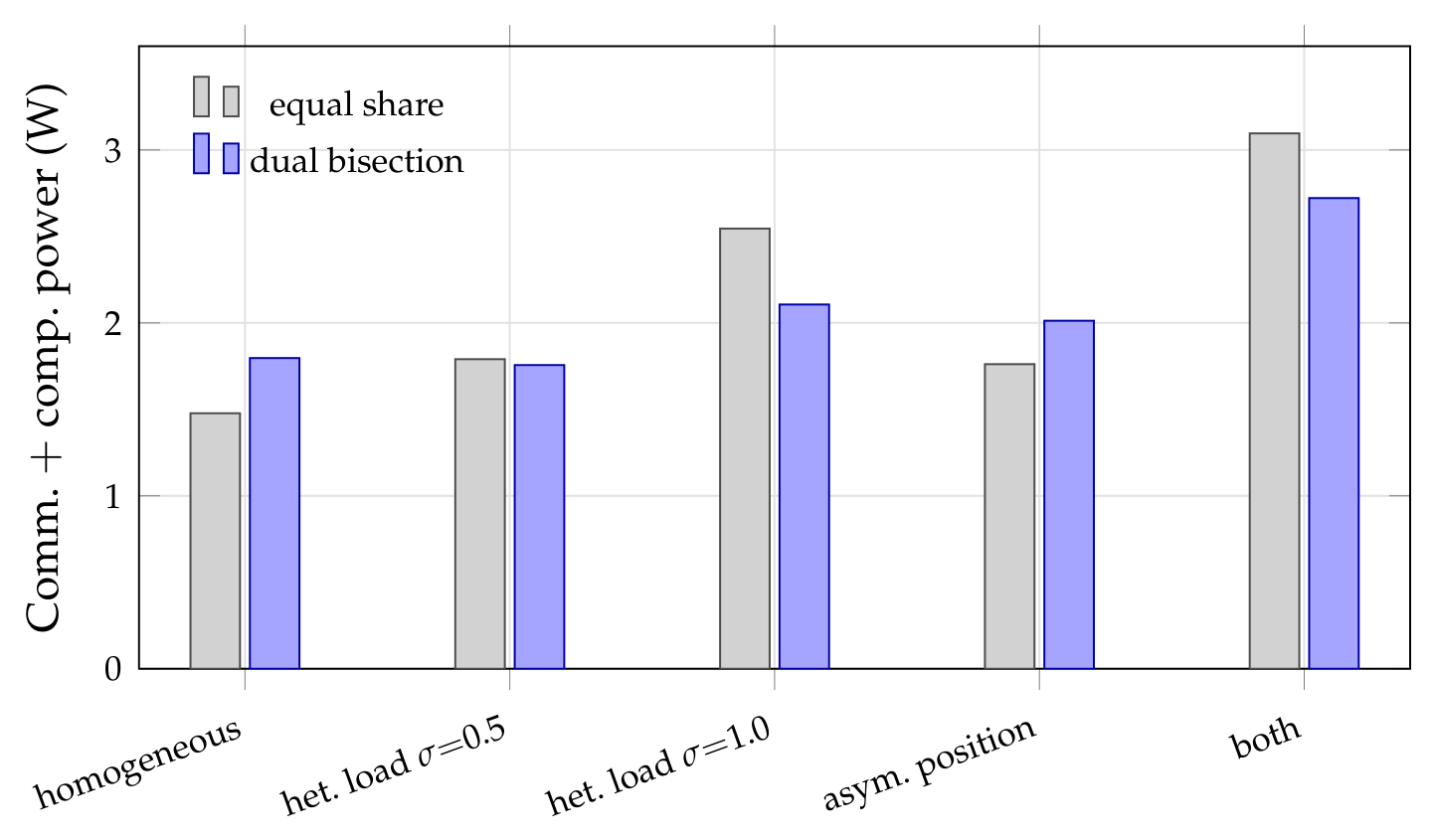
The ablation of Section 6.8 found the dual bisection of Section 5 slightly worse in closed loop than an equal share, which is a surprising result for an allocator that provably minimises the per-slot objective. Figure 9 resolves it: the ablation was run in a homogeneous scenario, where there is very little for a differential allocator to exploit.

We repeated the comparison with per-robot mean loads drawn log-normally (spread $\sigma \in \{0.5,1.0\}$, fleet total preserved) and with the fleet clustered asymmetrically in one far quadrant. Under homogeneous load the equal share is indeed better, by 21.6%; asymmetric position alone does not change this (14.2% in favour of equal share), because a uniformly distant fleet is still uniform in the quantity that matters. But under load heterogeneity the ordering reverses decisively: at $\sigma =1.0$ the bisection is 17.3% better on ICT power and roughly halves the violation rate ($1.78$ vs. 3.14%), and with both heterogeneities together it is 12.1% better with violations of $4.35$ against 6.23%.

The conclusion, and the answer to the question of whether an equal share suffices, is that it depends on a property of the deployment rather than on the algorithm: equal share is adequate, indeed preferable, since it is free when robots carry comparable loads, and inadequate when they do not. Since a fleet with heterogeneous roles is the realistic case, we retain the bisection as the default and record that it is the homogeneous benchmark, not the allocator, that was misleading.

6.12. A Stronger Decoupled Baseline

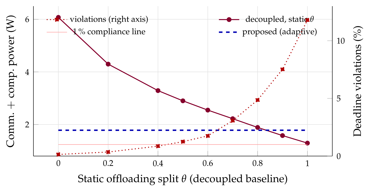
The decoupled baseline used so far fixes $\theta =0.5$, which is a weak opponent. Figure 10 sweeps the static split from 0 to 1 and reports both ICT power and violations, so that the best static split can be chosen offline with full knowledge of the operating point, an advantage the proposed policy does not have.

Optimising $\theta$ helps the baseline considerably. ICT power falls monotonically from $6.07$ $\mathrm{W}$ at $\theta =0$ to $1.29$ $\mathrm{W}$ at $\theta =1$, but violations rise monotonically too, from $0.14$ to 11.79%, so the usable range is bounded by compliance rather than by energy. Taking 1% violations as the compliance line, the best static split is ${\theta }^{\star }\approx 0.4$, giving $3.29$ $\mathrm{W}$ at 0.86%: a 46% improvement on the $\theta =0.5$ baseline reported in Table 4.

This changes the numbers, not the conclusion: the proposed policy’s $1.78$ $\mathrm{W}$ at 0.16% violations is still 46% below the best compliant static split, because any static $\theta$ pays in every slot where the channel or backlog departs from the average it was chosen for. That gap is precisely the value of conditioning on state.

6.13. Computational Overhead

Section 5 claims the scheme is light enough to run on the robot. We substantiate that by timing the decision rules directly, in isolation from the simulation harness, on an x86-64 core in interpreted CPython 3.12, a deliberately pessimistic environment, since a deployed node would be compiled.

Per robot per slot, the on-board rules cost $0.79$ $\mu$$\mathrm{s}$ (clock rule), $1.20$ $\mu$$\mathrm{s}$ (transmit rule) and $67.7$ $\mu$$\mathrm{s}$ (speed lookahead, dominated by its $H\times \left|\mathcal{V}\right|$ coverage-map evaluations), for a total of $69.7$ $\mu$$\mathrm{s}$, or 0.07% of a 100 $\mathrm{m}$$\mathrm{s}$ slot. Taking a conservative $30\times$ for interpreted-to-compiled and a further $4\times$ penalty for a $1.5$ $\mathrm{G}$$\mathrm{Hz}$ Cortex-A72 relative to the test core gives $9.3$ $\mu$$\mathrm{s}$ per slot, and even on a 400 $\mathrm{M}$$\mathrm{Hz}$ Cortex-M7 class core the estimate is 58 $\mu$$\mathrm{s}$, under 0.06% of the slot. The claim of a lightweight ROS node is therefore comfortable by three orders of magnitude, and the speed lookahead, the only non-trivial term, is also the one the ablation found dispensable.

The bandwidth bisection is a different matter: at $9.6$ $\mathrm{m}$$\mathrm{s}$ for $N=8$ in CPython it is by far the most expensive component. It is, however, a centralised computation that belongs at the access point rather than on the robots, it parallelises trivially across the inner per-robot searches, and the same $30\times$ compilation factor puts it near 320 $\mu$$\mathrm{s}$ on server-class hardware. Nothing in the per-robot budget depends on it.

6.14. Generality Check: Multiple Access Points and Edge-Capacity Limits

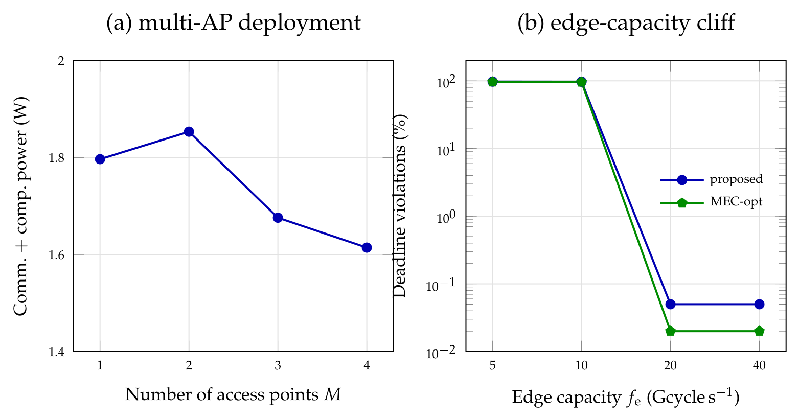
We emphasise before presenting numbers that this subsection is a scalability check on the single-AP algorithm of Section 4 and Section 5, not a new algorithm or a fourth contribution: no formulation or subproblem changes, and the question is only whether the design extends and how it behaves when it does. The model of Section 3 places one access point, co-located with one edge node, at the centre of the workspace. Industrial and low-altitude deployments are rarely so tidy: they involve several APs, several edge nodes, and robots that re-associate as they move. Two questions follow. Does the formulation extend, and does the policy still behave?

The formulation extends with essentially no change to Section 5. Adding APs $m\in \mathcal{M}$ makes the association ${\pi }_i\left(t\right)\in \mathcal{M}$ an additional per-slot decision; the bandwidth constraint (14e) becomes one constraint per AP, ${\sum }_{i:{\pi }_i\left(t\right)=m}{b}_i\left(t\right)\le 1$, so the dual bisection of Section 5 runs per AP on disjoint robot subsets; and the channel gain $h_i\left(t\right)$ is evaluated against the serving AP. Association itself is a discrete choice over a small set, resolved like the speed subproblem by enumeration, and in practice damped by the standard hysteresis that prevents ping-ponging. Several edge nodes enter as either a pooled queue of aggregate rate $M{f}_{\mathrm{e}}$ or as M independent queues, depending on whether the operator federates them. Nothing in Propositions 1 or 2 depends on M, because both are per-robot rules conditioned on the serving link.

Figure 11a reports the measured behaviour with M APs on a ring and per-AP bandwidth. ICT power falls from $1.80$ $\mathrm{W}$ at $M=1$ to $1.61$ $\mathrm{W}$ at $M=4$ and violations from $0.13$ to 0.04%, because a denser AP layout shortens the average serving distance; handovers remain modest (about two per robot per minute at $M=4$ with 3 dB hysteresis). Pooled and independent edge nodes were indistinguishable in these runs, which is expected: at this load the server is not the bottleneck, so how its capacity is partitioned does not matter.

That last observation sets up the more important experiment. Figure 11b constrains the edge node directly. Above 20 Gcycle s⁻¹ nothing changes, ICT power is flat to four significant figures because the offload path is limited by the radio, not the server. At and below 10 Gcycle s⁻¹ the system falls off a cliff: violations jump to 97% and mean latency to seconds, for the proposed policy and for MEC-opt alike. The cliff is not a failure of scheduling but of provisioning. Aggregate demand exceeds aggregate service capacity, and no policy can schedule its way out of that. It does, however, expose a real limitation of our routing rule, which we state rather than repair: the offload veto in (24) tests whether the server’s service time fits the deadline, but does not observe the server’s queue, so it keeps offloading into a saturated node instead of falling back to local execution. Making the veto congestion-aware, which in a multi-edge setting also means choosing among edge nodes by backlog, is a concrete and worthwhile extension.

6.15. Generality Check: Comparison with Learning-Based Policies

This subsection, likewise, is a robustness check rather than a contribution: it asks whether a learned routing decision changes the paper’s conclusion, using the same platform and evaluation protocol as the rest of Section 6. The baselines considered so far are rule-based. Since learned offloading policies are prominent in recent work [10,35,36], we add two. Single-agent RL learns the routing decision online by $ϵ$-greedy value learning over a discretised state (queue occupancy, channel quality) with a reward of negative slot energy plus a congestion penalty. Multi-agent RL extends the state with a fleet-congestion feature, so each robot conditions on the aggregate backlog as well as its own. Both use the same DVFS and transmit-power machinery as MEC-opt, isolating the routing decision as the learned component.

We are explicit about what these are and are not. They are lightweight tabular learners trained online, not reproductions of any particular published deep architecture, and a full DRL system with a deadline-shaped reward, a richer state encoding and offline pre-training would very likely do better than what we report. What they establish is narrower but still useful: that learning the routing decision from an energy-based reward, without an explicit feasibility mechanism, does not by itself deliver deadline compliance.

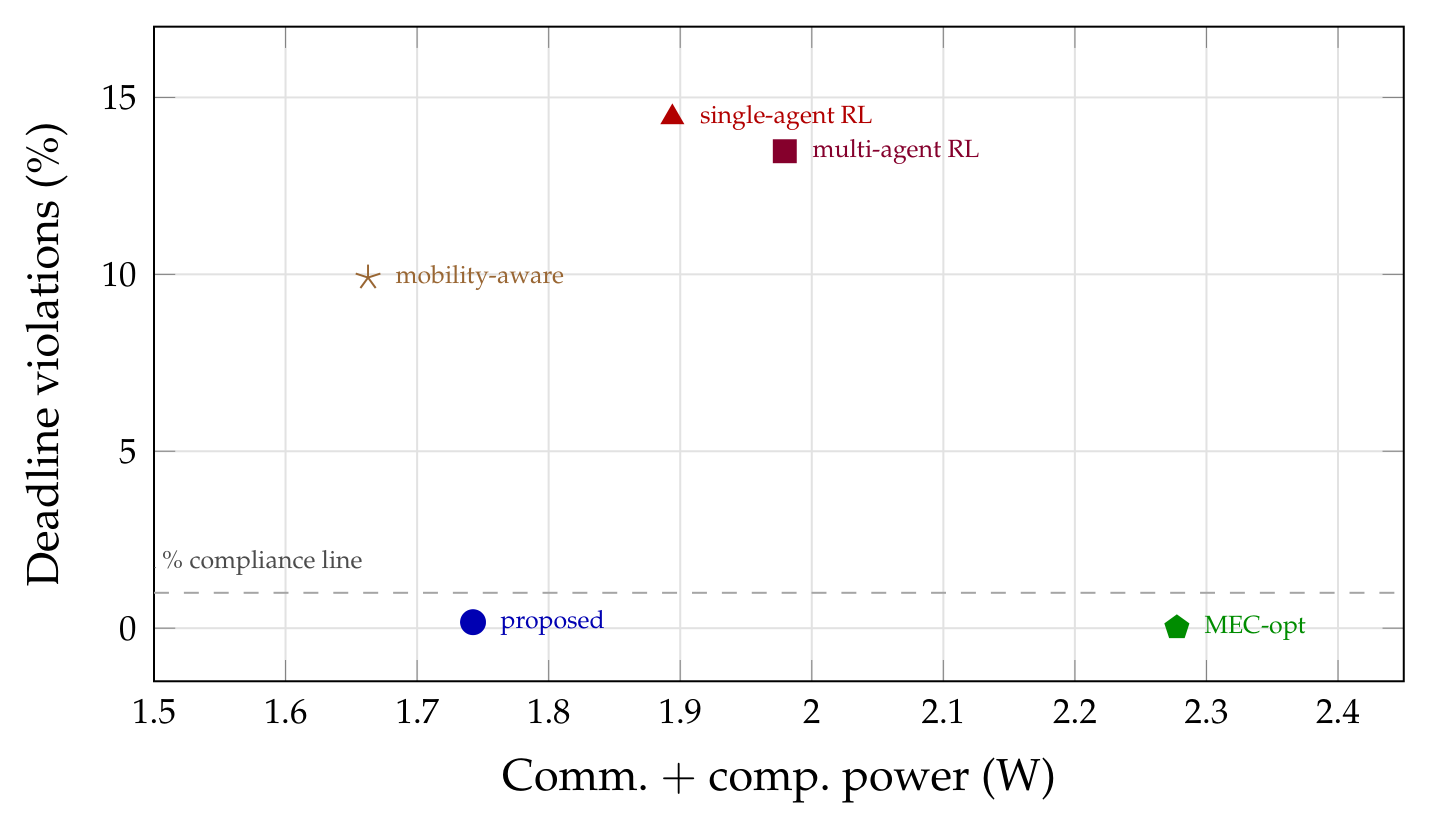
Figure 12 places all five policies in the energy–compliance plane. The learned policies reach competitive energy $1.89$ and $1.98$ $\mathrm{W}$ against $1.74$ $\mathrm{W}$ for the proposed policy but at $14.4$ and 13.5% deadline violations against 0.17%. The multi-agent variant is slightly better on compliance than the single-agent one, consistent with the fleet feature carrying genuine information about contention, and slightly worse on energy. The mechanism behind the gap is the same one identified in Section 5.6: an energy-shaped reward pushes the learner towards the offload path, which is cheaper per bit, and nothing in the value function represents the deadline of an individual task. Exploration compounds this, since an $ϵ$-greedy learner must occasionally take the infeasible action to discover that it is infeasible, a cost a feasibility floor never pays. We read this as supporting a hybrid rather than a competition: the drift rules and the learned policy are both routing heuristics, and either can be fitted with the floors of Section 5.6, exactly as Bi et al. combine drift with deep learning to retain a guarantee [10].

6.16. Sensitivity

We swept eight parameters one at a time around the default point (map error 0–8 dB; lookahead horizon 10–80 slots; circuit power 0–$0.4$ $\mathrm{W}$; shadowing decorrelation 4–16 $\mathrm{m}$; computational intensity 100–400 cycle bit⁻¹; deadline 0.3–$1.0$ $\mathrm{s}$; server rate 10–40 Gcycle s⁻¹; drag coefficient ${\beta }_2$ 0.5–2.2). The policy is insensitive to the map error, the horizon, the decorrelation length and ${\beta }_2$ (ICT power within $0.05$ $\mathrm{W}$ across each sweep), consistent with the lookahead null. Circuit power matters as the model predicts: ICT power moves from $1.84$ $\mathrm{W}$ at $P^{\mathrm{ckt}}=0$ to $2.30$ $\mathrm{W}$ at $0.4$ $\mathrm{W}$, with the guard suppressing marginal transmissions as the activation cost grows. Tightening the deadline to 300 $\mathrm{m}$$\mathrm{s}$ raises ICT power to $2.35$ $\mathrm{W}$ and violations to 0.95% as the floors engage. Two sweeps expose feasibility boundaries rather than graceful degradation: at L = 400 cycle bit⁻¹ the fleet’s aggregate demand exceeds the edge server’s capacity and violations jump to 94.5%, and halving the server rate to 10 Gcycle s⁻¹ produces the same collapse (90.3%). The routing veto does not currently observe the server’s queue, only its service time, so it fails to redirect work when the server itself saturates; making the veto congestion-aware is an easy and worthwhile extension, and we note it in Section 7.

7. Discussion

7.1. What the Results Support

The central claim the evaluation supports is narrower than “co-management saves energy”. It is that the joint objective, and specifically the ability to move work between the processor and the radio in response to their current marginal costs, is where the saving comes from. The evidence for this is Figure 5: the proposed scheme does not beat the greedy policy by using less of everything, but by using more radio and much less processor. Any scheme that fixes the split in advance, however well it then optimises each side, forgoes that.

A second, less obvious finding is how much of the benefit comes from the freedom to wait. Both the guard (23) and the queue-driven water level in (22) amount to permission to skip a bad slot. The myopic baseline is a controlled demonstration of the cost of not having that permission: it uses the same hardware and the same tradeoff intuition, and it pays 57% more power at high load purely because it insists on clearing each slot as it arrives.

7.2. Limitations

Six limitations are worth stating plainly, in order of consequence. Bursty arrivals degrade the deadline mechanism, not the energy tradeoff (Section 6.9): violations rise to roughly 9% and are insensitive to V, because the feasibility floors size against work already queued rather than anticipating a burst. An arrival-predictive floor is, in our view, the single most important extension. The offload veto is congestion-blind (Section 6.14): it checks the server’s service time but not its queue, so it does not fall back locally when the server saturates. The evaluation is simulated: the platform models are standard and the parameters representative, but only hardware contact can validate them; we expect the qualitative ordering of schemes to survive it, since that follows from the shape of the cost curves rather than their exact coefficients, but not the magnitudes. The coverage map is assumed given; a stale map degrades the speed rule towards a fixed-speed policy, failing safe rather than badly. Speed control is heading-following, not path-planning: routing the path itself through the coverage map is a substantially harder problem we have not attempted. Finally, as Section 5 already qualifies in detail, the clean $\left[O\right(1/V),O(V\left)\right]$ statement is for i.i.d. arrivals and channels; ergodic extensions hold with worse constants.

7.3. Practical Deployment

Three practical points are worth recording. First, the per-robot rules need only local state, so the scheme can be implemented as a ROS node [31] alongside the perception stack without a central scheduler; only the bandwidth allocation is shared, and equal-share was within 3% of optimal in our runs. Second, V is the only parameter that needs tuning in the field, and Figure 2 suggests a straightforward procedure: increase V until the measured latency reaches a chosen fraction of the deadline. Third, the DVFS set-points and the transmit-power granularity available on real hardware are coarse, and rounding (20) and (22) to the nearest available set-point costs little, since both objectives are flat near their optima.

8. Conclusions

Communication energy and computational energy on a wirelessly connected mobile robot are not separate budgets, and the robot’s own motion sets the exchange rate between them. We formulated their co-management as a long-run average energy minimisation under deadline, power, bandwidth and mission-progress constraints, and showed that a Lyapunov decomposition reduces the resulting stochastic, non-convex, mixed-integer problem to four per-slot subproblems cheap enough to run on the robot, a square-root clock rule, a guarded water-filling power rule, an energy-aware routing rule and a small enumeration over speeds, supplemented by per-task feasibility floors that supply the individual-deadline guarantee drift arguments do not. In a per-task evaluation against eight baselines, including learning-based policies, the scheme reduced combined communication and computation power by 25% relative to the strongest deadline-compliant competitor at equal mission progress and was alone in holding violations below 0.5% across the load range, where every baseline exceeded 16%; it extends without structural change to multi-AP, multi-edge deployments, in which a denser access-point layout reduces energy further. Three findings temper this and set the agenda: the channel-lookahead term contributed no measurable saving once the deadline machinery had removed the temporal slack that motion adaptation needs; the feasibility floors react to bursts rather than anticipating them, so bursty workloads degrade compliance and an arrival-predictive floor is the leading open problem; and the offload veto observes the edge server’s service time but not its queue, so it cannot fall back gracefully when the server saturates. Hardware validation, instrumenting a fleet to measure all three power terms at once, remains the most valuable next step and would settle what simulation cannot.

References

1. Mao, Y.; You, C.; Zhang, J.; Huang, K.; Letaief, K.B. A Survey on Mobile Edge Computing: The Communication Perspective. IEEE Commun. Surv. Tutor. 2017, 19, 2322–2358. [Google Scholar] [CrossRef] [Scilit]
2. Mach, P.; Becvar, Z. Mobile Edge Computing: A Survey on Architecture and Computation Offloading. IEEE Commun. Surv. Tutor. 2017, 19, 1628–1656. [Google Scholar] [CrossRef] [Scilit]
3. Groshev, M.; Baldoni, G.; Cominardi, L.; de la Oliva, A.; Gazda, R. Energy-Aware Joint Orchestration of 5G and Robots: Experimental Testbed and Field Validation. arXiv 2025, arXiv:2503.19613. [Google Scholar]
4. Huang, D.; Wang, P.; Niyato, D. A Dynamic Offloading Algorithm for Mobile Computing. IEEE Trans. Wirel. Commun. 2012, 11, 1991–1995. [Google Scholar] [CrossRef] [Scilit]
5. Mao, Y.; Zhang, J.; Letaief, K.B. Dynamic Computation Offloading for Mobile-Edge Computing with Energy Harvesting Devices. IEEE J. Sel. Areas Commun. 2016, 34, 3590–3605. [Google Scholar] [CrossRef] [Scilit]
6. Mao, Y.; Zhang, J.; Song, S.H.; Letaief, K.B. Stochastic Joint Radio and Computational Resource Management for Multi-User Mobile-Edge Computing Systems. IEEE Trans. Wirel. Commun. 2017, 16, 5994–6009. [Google Scholar] [CrossRef] [Scilit]
7. Kwak, J.; Kim, Y.; Lee, J.; Chong, S. DREAM: Dynamic Resource and Task Allocation for Energy Minimization in Mobile Cloud Systems. IEEE J. Sel. Areas Commun. 2015, 33, 2510–2523. [Google Scholar] [CrossRef] [Scilit]
8. Guo, M.; Wang, W.; Huang, X.; Chen, Y.; Zhang, L.; Chen, L. Lyapunov-Based Partial Computation Offloading for Multiple Mobile Devices Enabled by Harvested Energy in MEC. IEEE Internet Things J. 2022, 9, 9025–9035. [Google Scholar] [CrossRef] [Scilit]
9. Tong, Z.; Cai, J.; Mei, J.; Li, K.; Li, K. Dynamic Energy-Saving Offloading Strategy Guided by Lyapunov Optimization for IoT Devices. IEEE Internet Things J. 2022, 9, 19903–19915. [Google Scholar] [CrossRef] [Scilit]
10. Bi, S.; Huang, L.; Wang, H.; Zhang, Y.J.A. Lyapunov-Guided Deep Reinforcement Learning for Stable Online Computation Offloading in Mobile-Edge Computing Networks. IEEE Trans. Wirel. Commun. 2021, 20, 7519–7537. [Google Scholar] [CrossRef] [Scilit]
11. Kumar, K.; Lu, Y.H. Cloud Computing for Mobile Users: Can Offloading Computation Save Energy? Computer 2010, 43, 51–56. [Google Scholar] [CrossRef] [Scilit]
12. Cuervo, E.; Balasubramanian, A.; Cho, D.k.; Wolman, A.; Saroiu, S.; Chándra, R.; Bahl, P. MAUI: Making Smartphones Last Longer with Code Offload. In Proceedings of the 8th International Conference on Mobile Systems, Applications, and Services (MobiSys), San Francisco, CA, USA, 15–18 June 2010; pp. 49–62. [Google Scholar] [CrossRef] [Scilit]
13. Chun, B.G.; Ihm, S.; Maniatis, P.; Naik, M.; Patti, A. CloneCloud: Elastic Execution between Mobile Device and Cloud. In Proceedings of the 6th Conference on Computer Systems (EuroSys), Edinburgh, UK, 10–13 April 2011; pp. 301–314. [Google Scholar] [CrossRef] [Scilit]
14. Miettinen, A.P.; Nurminen, J.K. Energy Efficiency of Mobile Clients in Cloud Computing. In Proceedings of the 2nd USENIX Conference on Hot Topics in Cloud Computing (HotCloud), Boston, MA, USA, 22 June 2010. [Google Scholar]
15. Dinh, H.T.; Lee, C.; Niyato, D.; Wang, P. A Survey of Mobile Cloud Computing: Architecture, Applications, and Approaches. Wirel. Commun. Mob. Comput. 2013, 13, 1587–1611. [Google Scholar] [CrossRef] [Scilit]
16. Shi, W.; Cao, J.; Zhang, Q.; Li, Y.; Xu, L. Edge Computing: Vision and Challenges. IEEE Internet Things J. 2016, 3, 637–646. [Google Scholar] [CrossRef] [Scilit]
17. Taleb, T.; Samdanis, K.; Mada, B.; Flinck, H.; Dutta, S.; Sabella, D. On Multi-Access Edge Computing: A Survey of the Emerging 5G Network Edge Cloud Architecture and Orchestration. IEEE Commun. Surv. Tutor. 2017, 19, 1657–1681. [Google Scholar] [CrossRef] [Scilit]
18. Wang, S.; Zhang, X.; Zhang, Y.; Wang, L.; Yang, J.; Wang, W. A Survey on Mobile Edge Networks: Convergence of Computing, Caching and Communications. IEEE Access 2017, 5, 6757–6779. [Google Scholar] [CrossRef] [Scilit]
19. Pan, C.; Luo, Z.; Wang, K.; Feng, D.; Yue, X. Energy-Efficient Optimization for Integrated Sensing and Communication Assisted Cell-Free Urban Air Mobility. IEEE Trans. Veh. Technol. 2026, 75, 7756–7770. [Google Scholar] [CrossRef] [Scilit]
20. Lin, Z.; Niu, H.; He, Y.; An, K.; Zhong, X.; Chu, Z.; Xiao, P. Self-Powered Absorptive Reconfigurable Intelligent Surfaces for Securing Satellite-Terrestrial Integrated Networks. China Commun. 2024, 21, 276–291. [Google Scholar] [CrossRef] [Scilit]
21. Ma, Y.; Ma, R.; Lin, Z.; Miao, C.; Zhang, R.; Long, W. Distributed Split Single-Sideband Time-Modulated Arrays for Secure Communications. IEEE Internet Things J. 2024, 13, 23862–23875. [Google Scholar] [CrossRef] [Scilit]
22. Wang, Y.; Sheng, M.; Wang, X.; Wang, L.; Li, J. Mobile-Edge Computing: Partial Computation Offloading Using Dynamic Voltage Scaling. IEEE Trans. Commun. 2016, 64, 4268–4282. [Google Scholar] [CrossRef] [Scilit]
23. Chen, X.; Jiao, L.; Li, W.; Fu, X. Efficient Multi-User Computation Offloading for Mobile-Edge Cloud Computing. IEEE/ACM Trans. Netw. 2016, 24, 2795–2808. [Google Scholar] [CrossRef] [Scilit]
24. Zhang, W.; Wen, Y.; Guan, K.; Kilper, D.; Luo, H.; Wu, D.O. Energy-Optimal Mobile Cloud Computing under Stochastic Wireless Channel. IEEE Trans. Wirel. Commun. 2013, 12, 4569–4581. [Google Scholar] [CrossRef] [Scilit]
25. Guo, S.; Liu, J.; Yang, Y.; Xiao, B.; Li, Z. Energy-Efficient Dynamic Computation Offloading and Cooperative Task Scheduling in Mobile Cloud Computing. IEEE Trans. Mob. Comput. 2019, 18, 319–333. [Google Scholar] [CrossRef] [Scilit]
26. Liu, J.; Mao, Y.; Zhang, J.; Letaief, K.B. Delay-Optimal Computation Task Scheduling for Mobile-Edge Computing Systems. In Proceedings of the IEEE International Symposium on Information Theory (ISIT), Barcelona, Spain, 27 June–2 July 2016; pp. 1451–1455. [Google Scholar] [CrossRef] [Scilit]
27. Sardellitti, S.; Scutari, G.; Barbarossa, S. Joint Optimization of Radio and Computational Resources for Multicell Mobile-Edge Computing. IEEE Trans. Signal Inf. Process. Over Netw. 2015, 1, 89–103. [Google Scholar] [CrossRef] [Scilit]
28. Wang, F.; Xu, J.; Wang, X.; Cui, S. Joint Offloading and Computing Optimization in Wireless Powered Mobile-Edge Computing Systems. IEEE Trans. Wirel. Commun. 2018, 17, 1784–1797. [Google Scholar] [CrossRef] [Scilit]
29. Kehoe, B.; Patil, S.; Abbeel, P.; Goldberg, K. A Survey of Research on Cloud Robotics and Automation. IEEE Trans. Autom. Sci. Eng. 2015, 12, 398–409. [Google Scholar] [CrossRef] [Scilit]
30. Chowdhury, N.T.; Parasuraman, R. Edge Computing and its Application in Robotics: A Survey. arXiv 2025, arXiv:2507.00523. [Google Scholar]
31. Quigley, M.; Conley, K.; Gerkey, B.; Faust, J.; Foote, T.; Leibs, J.; Wheeler, R.; Ng, A.Y. ROS: An Open-Source Robot Operating System. In Proceedings of the ICRA Workshop on Open Source Software, Kobe, Japan, 12–17 May 2009; p. 5. [Google Scholar]
32. Rahman, A.; Jin, J.; Cricenti, A.; Rahman, A.; Panda, M. Motion and Connectivity Aware Offloading in Cloud Robotics via Genetic Algorithm. In Proceedings of the IEEE Global Communications Conference (GLOBECOM), Singapore, 4–8 December 2017; pp. 1–6. [Google Scholar] [CrossRef] [Scilit]
33. Rahman, A.; Jin, J.; Rahman, A.; Cricenti, A.; Afrin, M.; Dong, Y.n. Energy-Efficient Optimal Task Offloading in Cloud Networked Multi-Robot Systems. Comput. Netw. 2019, 160, 11–32. [Google Scholar] [CrossRef] [Scilit]
34. Sutton, R.S.; Barto, A.G. Reinforcement Learning: An Introduction, 2nd ed.; MIT Press: Cambridge, MA, USA, 2018. [Google Scholar]
35. Chinchali, S.; Sharma, A.; Harrison, J.; Elhafsi, A.; Kang, D.; Pergament, E.; Cidon, E.; Katti, S.; Pavone, M. Network Offloading Policies for Cloud Robotics: A Learning-Based Approach. Auton. Robot. 2021, 45, 997–1012. [Google Scholar] [CrossRef] [Scilit]
36. Wang, X.; Ning, Z.; Guo, S.; Wang, L. Mobility-Aware Computation Offloading for Swarm Robotics using Deep Reinforcement Learning. arXiv 2023, arXiv:2308.11154. [Google Scholar]
37. Liu, L.; Chen, J.; Brocanelli, M.; Shi, W. E2M: An Energy-Efficient Middleware for Computer Vision Applications on Autonomous Mobile Robots. In Proceedings of the 4th ACM/IEEE Symposium on Edge Computing (SEC), Arlington, DC, USA, 7–9 November 2019; pp. 59–73. [Google Scholar] [CrossRef] [Scilit]
38. Liu, L.; Zhong, R.; Willcock, A.; Fisher, N.; Shi, W. An Open Approach to Energy-Efficient Autonomous Mobile Robots. In Proceedings of the IEEE International Conference on Robotics and Automation (ICRA), London, UK, 29 May–2 June 2023; pp. 11569–11575. [Google Scholar] [CrossRef] [Scilit]
39. Baruffa, G.; Rugini, L. Resource Assignment Algorithms for Autonomous Mobile Robots with Task Offloading. Future Internet 2025, 17, 39. [Google Scholar] [CrossRef] [Scilit]
40. Goldsmith, A. Wireless Communications; Cambridge University Press: Cambridge, UK, 2005. [Google Scholar]
41. Neely, M.J. Stochastic Network Optimization with Application to Communication and Queueing Systems; Morgan & Claypool: San Rafael, CA, USA, 2010. [Google Scholar] [CrossRef] [Scilit]
42. Boyd, S.; Vandenberghe, L. Convex Optimization; Cambridge University Press: Cambridge, UK, 2004. [Google Scholar]
43. Bertsekas, D.P. Nonlinear Programming, 2nd ed.; Athena Scientific: Belmont, MA, USA, 1999. [Google Scholar]
Figure 1. Co-management architecture. Each robot arbitrates between three energy domains, processor, radio and drivetrain, using only its own queue state and the channel state reported by the access point. The three domains are coupled: the offloading split determines how much work each of the first two must absorb, and the speed determines what channel the radio will face over the next few seconds.
Electronics 15 03626 g001
Figure 2. Energy–delay tradeoff over the Lyapunov weight V, measured per-task. The deadline floors of Section 5.6 cap the latency growth that the unconstrained theory predicts, at the price of a violation rate that creeps upward with V.
Electronics 15 03626 g002
Figure 3. Average power per robot against offered load. Schemes marked † violate deadlines over part or all of the range (Figure 4).
Electronics 15 03626 g003
Figure 4. Per-task deadline violations against offered load. Unfinished tasks count as violations. The proposed policy holds below 0.5% across the range while every baseline exceeds its budget at high load.
Electronics 15 03626 g004
Figure 5. Decomposition of average power at the default operating point. The proposed policy shifts ICT work towards the radio, which the joint objective prices as the cheaper pipe.
Electronics 15 03626 g005
Figure 6. Average power per robot against fleet size at fixed total bandwidth (error bars: one standard deviation over seeds). The proposed policy is flatter and far less seed-sensitive than the threshold heuristics.
Electronics 15 03626 g006
Figure 7. Ablation: ICT power with each mechanism disabled (95% bootstrap intervals). The no-progress-queue variant completes zero waypoints; its low power reflects robots that have stopped working, not a better policy.
Electronics 15 03626 g007
Figure 8. Energy–delay tradeoff under departures from the analysed statistics. The monotone shape survives bursty arrivals and correlated fading; the deadline behaviour does not (see text).
Electronics 15 03626 g008
Figure 9. Equal-share versus dual-bisection bandwidth allocation. Equal share wins under homogeneous load; the bisection wins decisively once per-robot loads differ.
Electronics 15 03626 g009
Figure 10. Decoupled baseline with an offline-optimised static split. Energy falls and violations rise monotonically with θ ; the best compliant static split still sits well above the adaptive policy.
Electronics 15 03626 g010
Figure 11. (a) Multi-AP deployment: a denser layout reduces ICT power by shortening serving distances. (b) Edge-capacity constraint: above 20 Gcycle s−1 the offload path is radio-limited and capacity is irrelevant; below it, aggregate demand exceeds aggregate service and every policy fails together.
Electronics 15 03626 g011
Figure 12. Energy against deadline compliance. The learned policies reach competitive energy but miss deadlines by two orders of magnitude more than the proposed policy, because an energy-shaped reward contains no representation of individual task deadlines.
Electronics 15 03626 g012