Article

Few-Shot Active Radar Jamming Recognition Using Adaptive Confidence Dual-Branch Fusion Network with Full-Information Time–Frequency Features


1
School of Information and Communication, Guilin University of Electronic Technology, Guilin 541004, China
2
Guangxi Engineering Research Center for Intelligent Electromagnetic Spectrum Sensing and Control Technology, Guilin 541001, China
*
Author to whom correspondence should be addressed.
Electronics 2026, 15(16), 3576; https://doi.org/10.3390/electronics15163576
Submission received: 25 May 2026 / Revised: 21 July 2026 / Accepted: 7 August 2026 / Published: 11 August 2026
(This article belongs to the Special Issue Multi-View Learning and Applications)

Abstract

Active radar jamming recognition is an important technology in modern electronic warfare (EW). With the increasingly widespread application of Digital Radio Frequency Memory (DRFM) technology, the types of jamming have become more diverse. Meanwhile, in most non-cooperative confrontation scenarios, it is difficult to obtain large-scale labeled jamming samples. The commonly used methods for radar jamming signal recognition have some limitations. One is that they require a large number of jamming samples; the other is that their recognition performance degrades severely in few-shot scenarios. To address these limitations, an Adaptive Confidence Dual-Branch Fusion Network (ACDF-Net) is proposed for few-shot jamming recognition. The Short-Time Fourier Transform (STFT) is firstly used to obtain four-channel time–frequency features of the jamming signal, which fully retains the real part, imaginary part, amplitude, and phase information of jamming. Secondly, a dual-branch complementary representation learning network is well designed to extract jamming modulation characteristics and energy-phase characteristics. Finally, an adaptive confidence fusion method controlled by learnable parameters and a multi-task supervised learning paradigm are introduced, which improve recognition accuracy and make the network more robust. A mixed dataset containing 15 types of radar active jamming (including 8 single jamming types, 3 composite jamming types, and 4 real measured jamming types) is established to verify the proposed method. Multi-dimensional validation experiments are conducted, including few-shot performance comparison under different training set proportions (3~11%), per-class recognition performance analysis, measured data generalization validation, and ablation studies of core modules. In few-shot scenarios, the OA of ACDF-Net reaches 92.81% under 3% training data proportion, which is better than the comparison algorithms. More comparative experiments show that the proposed method is better than the comparison methods. The proposed method provides an effective solution for radar active jamming recognition in few-shot and complex electromagnetic environments, which exhibits high feasibility for practical engineering applications.

1. Introduction

Radar serves as a crucial instrument in electronic warfare (EW), possessing the capability to execute tasks such as target detection, localization, identification and tracking [1,2,3,4]. However, it can also be affected by different types of jamming signals [5]. The introduction of Digital Radio Frequency Memory (DRFM) technology has made jamming signals more diverse, which is a challenge to the normal functioning of radar [6,7]. The problem of accurate and reliable recognition of radar jamming signals in complex electromagnetic conditions has always been a core research focus in the field of electronic countermeasures [8], and the ability of radar jamming recognition is the prerequisite of taking appropriate countermeasures.
The conventional active radar jamming techniques are divided into two major categories: suppressive jamming [9] and deceptive jamming [10,11]. In suppressive jamming, high-power noise-like signals are used to saturate the operating frequency of the target radar, thus preventing the radar from detecting the echo of the target. It has benefits such as wide area coverage, simple implementation, and high adaptability. However, it is easily intercepted, leading to the exposure of the jammer’s location, and requires excessive transmit power. The DRFM-based deceptive jamming [12,13] performs the interception of radar signals, accurate reproduction and flexible retransmission of the radar-transmitted signals by using large-scale false target jamming, which can provide false target data to the radar. In contrast to suppressive jamming, deceptive jamming merely needs to digitally manipulate the recorded radar waveforms to generate deceptive signals without high transmission power. Therefore, it is characterized by low transmission power, good concealment, high jamming targeting and strong deception. Based on the above principles, these two types of jamming are widely applied, and the radar’s ability to detect and track targets in actual combat will be weakened [14].
Besides the development of jamming techniques, radar interference mitigation has also been extensively investigated at the waveform and system levels. Representative approaches include mutual interference mitigation for LFMCW radars, orthogonal waveform design, and nonlinear frequency-modulated (NLFM) waveform optimization [15,16,17]. These methods improve radar coexistence capability and robustness against interference from the transmitter and system perspectives. However, they mainly focus on interference avoidance and suppression rather than the subsequent recognition of jamming types.
Many traditional radar jamming recognition methods rely on abundant prior knowledge and expert experience. The methods consist of two steps: the first step is to select designed features from the observed jamming signals, and the second is to use the pre-determined classifier for feature matching and jamming recognition. For example, Greco et al. [18] proposed a deceptive jamming recognition method based on the Adaptive Coherence Estimator (ACE) and the Generalized Likelihood Ratio Test (GLRT). Xing et al. [19] used the confidence distribution as a feature, and adopted the partially observable Markov decision process (POMDP) for jamming identification; Bandiera et al. [20] proposed an adaptive decision-making method using GLRT for distinguishing different jamming signals. Zhao et al. [21] established a classic linear model using GLRT for radar real targets and deceptive jamming identification; Su and Gao [22] obtained information from the time domain, frequency domain, and polarization domain of the jamming signal based on machine learning classifiers. Hao et al. [23] applied time–frequency atomic decomposition technology and support vector machine (SVM) to detect dense false target jamming and effectively distinguished the difference between target echoes and dense false target jamming with Gabor atomic time–frequency parameters.
However, the above methods based on handcrafted features also have many drawbacks that limit their practical engineering deployment. Firstly, the feature extraction process is more complicated, and the selection of thresholds and feature comparison require more accumulated experience. Therefore, it lacks robustness under varying conditions. Secondly, in certain complex electromagnetic environments, the target echoes and jamming signals overlap or alias in the time domain and frequency domain. Moreover, it is not easy to obtain relevant target information and form a comprehensive expert experience database with the various forms of jamming signals, which also makes the traditional methods unsuitable for engineering practice.
Signal-processing-based jamming detection and suppression methods have also attracted considerable attention. Sparse reconstruction-based interference reduction, bi-level l1 optimization, and TQWT-domain interference mitigation have demonstrated effectiveness in improving radar robustness and signal recovery capability under interference conditions [24,25,26]. Nevertheless, these approaches primarily address interference suppression rather than the recognition and classification of different jamming types under limited training samples.
In recent years, radar jamming recognition has received a lot of attention from researchers, thanks largely to the advent of deep learning technology. Many researchers have utilized deep learning techniques to identify and classify radar jamming signals, mainly stemming from the feature learning and representation capabilities of convolutional neural networks (CNNs) [27,28,29,30,31]. More recently, transformer-based radar perception models have also attracted increasing attention. Cheng and Cao [32] proposed TransRAD, which employed a retentive vision transformer to enhance radar object detection performance through long-range dependency modeling. Cheng et al. [33] further showed that radar measurements possess characteristics substantially different from image-like inputs through radar–camera co-calibration studies, highlighting the necessity of radar-oriented representation learning strategies. Lu et al. [34] reformulated the jamming perception task as an oriented object detection problem, achieving simultaneous jamming classification and parameter estimation via the YOLOv8-OBB network. Kong et al. [35] provided an active deceptive jamming recognition algorithm based on an attention mechanism-augmented residual CNN. Hou et al. [36] designed a multi-scale attention network for target and multi-type jamming recognition. Chen et al. [37,38] constructed multi-channel and multi-domain fusion networks to improve compound jamming recognition under low-JNR conditions. Li et al. [39] proposed a versatile multi-feature extraction front-end module (MFE-STN) for SAR deception jamming false target recognition, enhancing generalization to unseen jamming types. Qian et al. [40] developed a CNN-based radar jamming detection method combining time–frequency analysis for jamming presence detection and type recognition.
Although these deep learning-based methods have shown good performance, they require a large amount of jamming data for training. In practical engineering, it is more difficult to obtain large-scale jamming sample data. Moreover, due to the complexity of the electromagnetic environment itself, the features also change significantly under different working conditions. All these factors will affect the recognition accuracy and robustness of the above methods. Therefore, how to design effective radar active jamming identification methods under a small number of samples has become a current research hotspot issue, which has important practical significance.
Recently, few-shot active radar jamming recognition has been studied [41,42,43,44]. These few-shot approaches can achieve effective jamming recognition with limited training samples to a certain extent. As an example, Luo et al. [45] developed a few-shot jamming identification network integrating time–frequency self-attention mechanism and global knowledge distillation which balances the overall information of the time–frequency spectrum of the jamming signal and the real-time performance of the jamming identification network. Lv et al. [46] developed a radar active deceptive jamming recognition algorithm based on transfer learning–Weighted Ensemble Convolutional Neural Network (WECNN). Luo et al. [11] designed a few-shot jamming recognition program, which uses cross-modal refinement, enhancing the accuracy and robustness of the jamming classifier by identifying the slight difference in the jamming signal. However, in the actual electromagnetic environment, these methods lack robustness and generalizability, and have poor performance in various numbers of training samples and diverse Jamming-to-Noise Ratio (JNR) scenarios.
To address the limitations, this paper proposes an ACDF-Net to achieve high-performance radar active jamming recognition in few-shot scenarios. Firstly, the STFT is used to construct the four-channel time–frequency feature vector dataset, which preserves the real part, imaginary part, amplitude, and phase of the radar jamming signal, and differences among the various types of jamming characterized by distinct modulation schemes and power levels. Secondly, a dual-branch complementary representation learning architecture is designed with Residual Network 18 (ResNet18), which is developed to extract the joint modulation features and energy-phase features independently to enhance the discriminability of the features. Ultimately, a self-adaptive confidence fusion approach is employed, incorporating learnable parameters that enable the two branches to contribute distinctively in the recognition process. In addition, a multi-task supervised training mechanism that jointly optimizes the independent losses of the two branches and the final combined loss is proposed. Unlike conventional approaches that directly concatenate multi-domain features or employ fixed fusion strategies, the proposed ACDF-Net integrates complementary four-channel representations with adaptive confidence-guided fusion under multi-task supervision. This design enables the model to exploit branch-specific reliability and improve robustness for few-shot radar jamming recognition. This approach enables the model to demonstrate greater robustness and generalization capabilities in few-shot scenarios. The key contributions of this work are summarized as follows:
(1)
A four-channel STFT-based time–frequency representation, including the real part, imaginary part, amplitude, and phase information of radar jamming signals, is constructed. Combined with a dual-branch ResNet18 framework, complementary feature learning is achieved to improve the discriminative capability of different jamming types under few-shot conditions.
(2)
An adaptive confidence fusion strategy with multi-task supervision is proposed to dynamically fuse the outputs of the two branches according to their prediction reliability. This strategy alleviates overfitting in few-shot scenarios and improves the robustness of the proposed model under varying JNR conditions.
(3)
A mixed dataset containing simulated and measured jamming signals is established for experimental validation. Extensive experiments under different few-shot settings demonstrate the effectiveness and practical potential of the proposed ACDF-Net for radar jamming recognition.
The remaining part of this article is organized as follows. Section 2 presents the generation principle of radar signals and jamming signals. Section 3 describes the proposed method in detail. Section 4 contains the results of the experiment and provides a discussion. Finally, Section 5 concludes this paper.

2. Data Generation Methods

In this section, the generation methods of radar echo signals and jamming signals are introduced, which are used to construct the experimental dataset used in this paper. In the field of EW, a radar transmits radio frequency signals into the target area. During spatial propagation, these signals are distorted by jamming signals and noise signals before being received by the radar receiver.
The time-domain composite signal captured by the radar receiver can be split into three distinct components: the target echo, the jamming signal, and additive noise. Its mathematical expression is given as
S ( t ) = s _ r ( t ) + J _ m ( t ) + n ( t )
where S ( t ) stands for the full composite time-domain signal received by the radar; s _ r ( t ) is the target echo, which carries critical information about the target including its range, velocity, and angle; J _ m ( t ) represents the jamming signal that can be a single jamming type or a mix of multiple types; and n ( t ) is the noise from the radar receiver and the surrounding environment, which can be approximated as additive white Gaussian noise.

2.1. Radar Echo Signal

In this work, the linear frequency modulation (LFM) signal is used as the transmission waveform for radar system. The normalized expression of the LFM signal is written as
X ( t ) = A ·   r e c t ( t T ) e j 2 π ( f 0 t + γ 2 t 2 )
where A is the amplitude of the radar-transmitted signal, which directly determines the maximum theoretical detection range of the radar. T stands for the pulse width of the signal. f 0 is the carrier frequency of the radar signal, which defines the radar’s operating frequency band and has a direct impact on how the radar signal propagates in space, as well as the scattering characteristics of the target. γ refers to the linear frequency modulation slope of the LFM signal. The corresponding signal bandwidth is calculated as B = γ · T . r e c t ( ) is the rectangular window function, which defines the effective duration of the LFM pulse.

2.2. Jamming Signals

Radar active jamming can be classified into two types, suppressive jamming and deceptive jamming, and the composite jamming consists of these two types of jamming. In the dataset, three types of jamming are included. The methods for each type of jamming are derived from references [11,45,46,47].
In the simulation dataset, distance deceptive jamming (DDJ), dense false target jamming (DFTJ), interrupted sampling repeater jamming (ISRJ), and smeared spectrum jamming (SMSP) are categorized as deceptive jamming, whereas barrage jamming (BJ), comb spectrum jamming (COMB), and radio frequency noise jamming (RNJ) are categorized as suppressive jamming. Different jamming types have diverse working principles and technical parameters.
BJ suppresses the entire frequency band with noise. COMB suppresses the wide frequency band with discrete frequency points of the comb pattern. RNJ uses broadband radio frequency noise to drown out the target echoes.
All types of deceptive jamming are generated based on DRFM technology, which can generate coherent false targets against the radar. DDJ can deceive in distance. ISRJ can generate distributed false targets in distance, and DFTJ can generate false targets exceeding the order of magnitude of the pulse repetition period, causing overload to the radar detection. Smart noise jamming (SNJ) is a typical DRFM-based composite jamming, generated by convolving the intercepted radar signal with weighted Gaussian noise. It combines the suppression effect of noise jamming and the coherent gain of deceptive jamming, making it a widely used jamming method in practical electronic warfare.
Furthermore, this paper also combines a single jamming pattern with other jamming signals for jamming superposition, forming three types of composite jamming: DDJ + ISRJ, DDJ + SNJ, and DFTJ + SNJ. Due to the difficulty in extracting jamming characteristics, the difficulty of jamming identification increases. Based on this, in the next section, a learning radar jamming identification method based on few-shot is proposed to improve the robustness of the radar system in the presence of strong jamming.
All the experimental datasets used in this paper are generated following the physical properties of the given radar jamming signals. The dataset has diverse parameter settings, which can effectively support the performance comparison of different jamming recognition methods.

3. Proposed Method

3.1. Architecture of the Proposed ACDF-Net

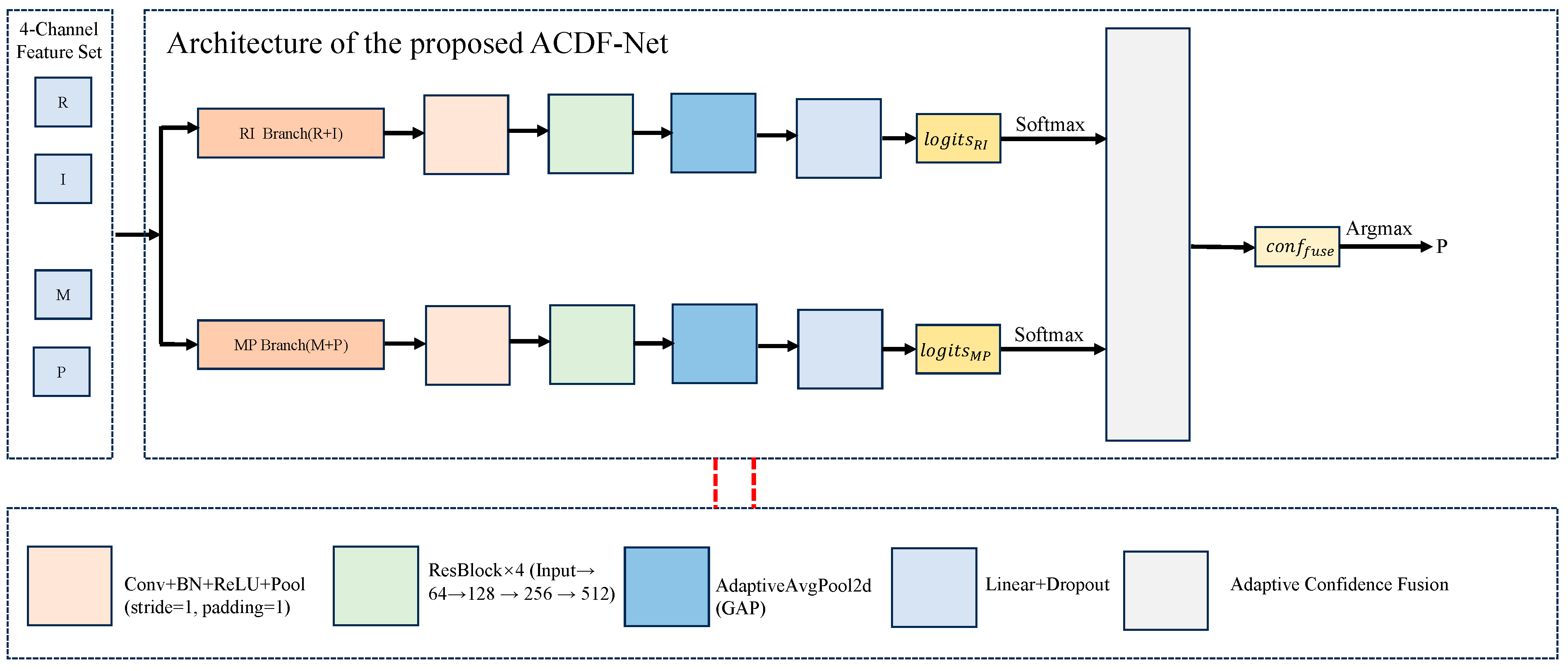
This section comprehensively introduces the radar jamming recognition principle of ACDF-Net. The preprocessing of radar jamming signals and the network structure are shown in Figure 1 and Figure 2. As shown in Figure 2, the ACDF-Net consists of four connected parts: a feature input layer, a dual-branch complementary representation learning module, an adaptive confidence fusion module, and a recognition output layer. The complete forward propagation workflow of the network is as follows:
(1)
A one-dimensional time-domain jamming signal is given, which is processed by using the STFT to get a time–frequency feature map of size 4 × 100 × 247 .
(2)
The four-channel time–frequency feature tensor is split along the channel dimension into two independent branches. The first two channels (real and imaginary parts of the complex time–frequency matrix) are used as the real–imaginary modulation branch, and the last two channels (amplitude and phase) are used as the amplitude–phase energy branch.
(3)
Each branch independently extracts discriminative features through 8 residual blocks organized into 4 layers, following the standard ResNet18 architecture, and maps the features to 16-dimensional raw recognition logits through the Global Average Pooling (GAP) layer and Fully Connected (FC) layer.
(4)
The recognition confidence scores of the two branches are weighted and fused via a learnable parameter α to obtain the final fused confidence.
(5)
The total loss is calculated by the cross-entropy loss function, which takes the independent logits of each branch and the fused logits as inputs respectively. The sum of the three losses is used to optimize all trainable parameters of the network.
During inference, the model takes the preprocessed radar jamming signal as input, performs forward propagation through the dual-branch network and adaptive confidence fusion module, and outputs the final predicted class label corresponding to the maximum value in the fused recognition confidence distribution.

3.2. STFT-Based Feature Extraction

3.2.1. Amplitude Normalization

The modulation of radar jamming signals can be seen in four parts: real part, imaginary part, amplitude and phase, which can be defined as a four-channel time–frequency feature vector. This vector is used to represent the modulation information of the jamming signal.
Given a one-dimensional complex-valued jamming signal J C 1 × N , the amplitude normalization is performed on it, as shown in Equation (3). It is to eliminate the impact of absolute energy variation on features. These variations come from signals with different JNR. This step makes features comparable.
J n o r m = J m a x ( | J | )
where | J | is the complex magnitude of the input signal, and J n o r m denotes the normalized baseband signal.

3.2.2. Time–Frequency Feature Construction

STFT is employed to extract features, which converts a 1D time-domain waveform into a 2D time–frequency spectrogram. It works by sliding a fixed-size window across the input signal, which splits the non-stationary time series into multiple short time segments. Fourier transform is applied to each segment to generate the time–frequency representation of the signal. Its mathematical expression is written as
S T F T ( n , k ) = m = 0 L w i n 1   J n o r m ( n + m ) w ( m ) e j 2 π k m N F F T
where w ( ) is the window function, n denotes the time index, and k is the frequency index. L w i n denotes the window length, and N F F T is the number of FFT points. The parameter configurations for STFT discussed in this article are set as follows: f s = 20   M H z , the number of FFT points of N F F T = 100 , the window function is Hann window with the length of L w i n = 32 , and overlap length between windows is set as L o v e r l a p   = 24 .
A complex-valued time–frequency matrix is obtained after STFT processing. Four features are extracted from this matrix, real part (R), imaginary part (I), amplitude (M), and phase (P). These four features form a four-channel time–frequency feature dataset. All four parameters must undergo normalization, and are stacked and concatenated along the channel dimension. This step produces a 4 × 100 × 247 four-channel time–frequency feature tensor which is fed into the dual-branch network for subsequent processing.
The real and imaginary channels preserve the complete complex-valued representation of the STFT coefficients and retain modulation-related characteristics of radar jamming signals. The amplitude and phase channels explicitly characterize energy distributions and phase evolution patterns in the time–frequency domain. Since different jamming types may exhibit discriminative characteristics in different feature domains, combining these complementary representations enables more comprehensive feature extraction and improves the distinguishability of jamming signals under few-shot conditions.

3.3. Dual-Branch Complementary Representation Feature Learning Backbone

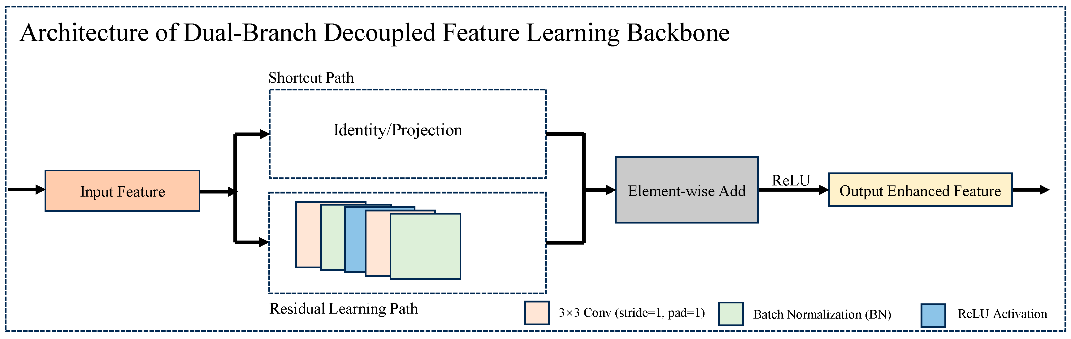
Considering the differences between the real–imaginary modulation features and amplitude–phase energy features from the 4-dimensional STFT time–frequency tensor, a dual-branch complementary representation learning structure is designed as shown in Figure 2. The two branches adopt the same network architecture, while their weight parameters are updated independently during training. This structure is named the dual-branch complementary representation learning backbone, and each branch uses ResNet18 as its base network, thus ensuring that both branches have equal abilities. The residual blocks in ResNet18 are used to build the dual-branch network in Figure 3.
The forward propagation formulas of the block in Figure 3 are given as follows:
h 1 = B N ( C o n v 3 × 3 ( x ) ) h 2 = R e L U ( h 1 ) h 3 = B N ( C o n v 3 × 3 ( h 2 ) ) h 4 = h 3 + Projection ( x ) y r e s = R e L U ( h 4 )
where x denotes the input feature of the residual block; h 1 is the intermediate feature after the first 3 × 3 convolution and batch normalization, which completes the first spatial feature extraction and distribution normalization of the input; h 2 is the nonlinear activation output of h 1 , which introduces nonlinear mapping capability to the residual block; h 3 is the intermediate feature after the second 3 × 3 convolution and batch normalization, which completes the second round of deep feature extraction on the basis of the activated features; h 4 is the feature after residual skip connection fusion, which adds the original input projection feature and the second convolution output feature to form the core residual mapping; y r e s is the output feature of the block; C o n v 3 × 3 ( ) is the 3 × 3 2D convolution operation with a default stride of 1; B N ( ) denotes batch normalization; and Projection ( x ) denotes the projection transformation. It uses 1 × 1 convolution to adjust the channel number or feature size when input and output have different channel counts or dimensions.
Each branch of the backbone strictly follows the standard ResNet18 network configuration, customized for the 2 × 100 × 247 time–frequency feature input. The detailed layer parameters and output dimensions of the dual-branch backbone are summarized in Table 1.
The core advantage of this residual block is optimized gradient propagation during training. The gradient of the feature with respect to the loss function is expressed as
L x = L y r e s ( ( h 3 + Projection ( x ) ) x ) = L y r e s ( h 3 x + Projection ( x ) x )
From the formula, it can be clearly seen that the gradient can be split into two parts: the gradient of the residual path and the gradient of the skip connection. Even if the gradient of the residual path is close to zero, the gradient of the skip connection can still prevent gradient disappearance. This step solves the problem of gradient disappearance in deep neural networks. It also allows the model to converge well even in few-shot.

3.4. Adaptive Confidence-Level Fusion Strategy

An adaptive confidence fusion method based on learnable parameters is proposed to obtain the final recognition result. In this strategy, the normalized recognition confidence scores of the two branches are weighted and summed directly, which avoids overfitting caused by feature-level fusion and enables each branch to be trained independently. Meanwhile, the fusion proportion of each branch can be automatically adjusted according to different types, which adaptively balances the contribution of the two branches according to their overall recognition confidence.
The Softmax function is adopted to convert the 16-dimensional raw recognition logits output by the two branches into normalized recognition confidence distributions. This function maps the unbounded logits to the interval [0, 1], and the sum of confidence values over all categories is constrained to 1. The mathematical expressions are given as
c o n f R I = S o f t m a x ( l o g i t s R I )
c o n f M P = S o f t m a x ( l o g i t s M P )
where l o g i t s R I and l o g i t s M P denote the raw outputs of the two branches before Softmax normalization, while c o n f R I and c o n f M P represent the corresponding confidence distributions. The normalized confidence distributions of the two branches are then weighted and fused using α .
c o n f f u s e = α c o n f R I + ( 1 α ) c o n f M P
where α ∈ [0, 1] denotes the learnable adaptive fusion coefficient. By dynamically adjusting the contribution of each branch according to the recognition confidence, a sigmoid operation is applied to constrain its value during optimization. The proposed strategy exploits complementary information while avoiding the overfitting risk associated with feature-level fusion under few-shot conditions.
To ensure that both branches can independently learn discriminative representations while optimizing the final fused prediction, the branch-wise cross-entropy losses are defined as
L C E ( l o g i t s , y ) = 1 N i = 1 N   c = 1 16   [ ( 1 ϵ ) I ( y i = c ) + ϵ 16 ] l o g ( S o f t m a x ( l o g i t s i , c ) )
where N denotes the number of samples in the batch, I ( ) denotes the indicator function, and ϵ is the label smoothing coefficient set to 0.12. Label smoothing assigns a small non-zero probability to non-target category labels, which converts the original hard 0/1 one-hot labels into soft labels with a small tolerance. To alleviate overfitting under few-shot conditions, label smoothing cross-entropy is adopted for supervising both individual branches.
Since the fused output is directly obtained in the probability space without label smoothing, the fusion loss is formulated as
L ( F u s e ) = 1 N n = 1 N c = 1 C y n , c l n ( c o n f ( f u s e , n , c ) )
where N denotes the batch size, C is the total number of categories, y n , c is the one-hot encoded ground-truth label, and c o n f ( f u s e , n , c ) represents the fused confidence corresponding to the c -th category of the n -th sample.
Accordingly, the overall optimization objective is expressed as
L ( t o t a l ) = L C E ( l o g i t s R I , y ) + L C E ( l o g i t s M P , y ) + L ( F u s e )
The proposed multi-task supervision strategy jointly optimizes the two individual branches and the fused prediction, enabling each branch to learn effective discriminative features while improving the final recognition performance and robustness under few-shot conditions.

3.5. Model Training and Inference Process

The complete training procedure is detailed in Algorithm 1.
Algorithm 1 Training procedure of ACDF-Net
Require:
       Radar jamming dataset D with labels Y
       Training ratio r
       Maximum epochs E _ m a x
       Batch size B
       Early stopping patience P Ensure:
       Optimal network weights θ *
       Recognition results on test set
1: Randomly initialize model parameters θ .
2: Split D into training, validation and test sets.
3: Initialize AdamW optimizer.
4: Set V b e s t   = 0 and M S t o p   = 0 .
5: for epoch = 1 to E _ m a x do
6:         Set model to training mode.
7:         for each mini-batch do
8:                     Forward propagation
9:                     compute L t o t a l .
10:                   Backpropagate gradients and update θ .
11:         end for
12:         Evaluate validation accuracy V a .
13:         if V a   > V b e s t then
14:                    Save current model.
15:                     V b e s t   = V a .
16:                     M S t o p = 0 .
17:         else
18:                     M S t o p = M S t o p   + 1 .
19:                    if M S t o p   P then
20:                          Break
21:                    end if
22:         end if
23: end for
24: Load the optimal model weights.
25: Perform inference on the test set.
26: Output Jamming Recognition results.
In the inference stage, the optimal model weights saved during training are loaded, and only forward propagation is executed without backpropagation or parameter updates. The full inference workflow has these steps. The trained optimal model weights are loaded to evaluation mode. STFT and amplitude normalization are performed on the input 1D radar jamming signal to generate a 4 × 100 × 247 feature tensor, which is then fed into the model; after forward propagation through the dual branches and adaptive confidence fusion, the recognition probability distribution can be obtained, which takes the index of the maximum value in this distribution as the final identified jamming type.

4. Experiment and Results

This section first describes the parameter settings of the experimental dataset, which compares the proposed method with other mainstream high-performance algorithms, and finally conducts ablation studies on each core module of the proposed method to verify its effectiveness and superiority.

4.1. Datasets

Our experimental dataset includes three types of data: radar transmission signals, simulated jamming signals, and real measured jamming signals which cover many common jamming types in real radar confrontation scenarios. The main parameters of these jamming signals are listed in Table 2. For the same jamming type, simulated and real measured signals use the same parameter settings, thus ensuring that the feasibility and effectiveness of our proposed method can be verified.
All 1D time-domain signals in the dataset cover 15 types of jamming signals and 1 type of non-jamming signal. Each signal has 2000 sampling points in length. The 15 jamming types are divided into three groups: 8 types of simulated single jamming, 3 types of simulated composite jamming, and 4 types of measured jamming signals. As shown in Table 2, the parameters of the four types of measured jamming signals match those of the corresponding four simulated single jamming signals. To keep all samples uniform, each type has 500 independent samples. The JNR of each jamming sample is randomly chosen between 30 dB and 60 dB. This matches the JNR changes in real electromagnetic environments.
It should be noted that all radar echoes and jamming signals considered in this study are represented in the equivalent baseband domain after down-conversion. Therefore, carrier frequency, RF front-end characteristics, and analog filtering processes are not explicitly modeled, and the bandwidth parameters listed in Table 2 refer to the effective baseband processing bandwidths.
Since this work focuses on the jamming recognition stage, the jamming signals are assumed to have entered the receiver processing chain and to overlap with the receiver processing bandwidth. Consequently, the frequency-overlap condition required for recognition is satisfied. RF propagation and front-end coupling effects are beyond the scope of this study.
Composite jamming samples are generated by randomly superimposing two single jamming signals with different JNR values, making the constructed scenarios more consistent with practical electromagnetic confrontation environments. During dataset generation, the signal-to-noise ratio (SNR) of the radar echo is fixed at 0 dB, while the jamming power is adjusted relative to the noise power to produce samples with JNR values ranging from 30 dB to 60 dB, thereby representing different interference intensities. The target is randomly located within the radar’s maximum unambiguous range of 15 km, corresponding to a round-trip time delay of 100 μs, and the exact position of the real target echo in each sample is unknown. Since all signals are represented in the equivalent baseband domain after down-conversion, the signal-to-interference-plus-noise ratio (SINR) is not independently defined or controlled in this study. These settings are intended to approximate the practical operating conditions encountered in real radar systems.
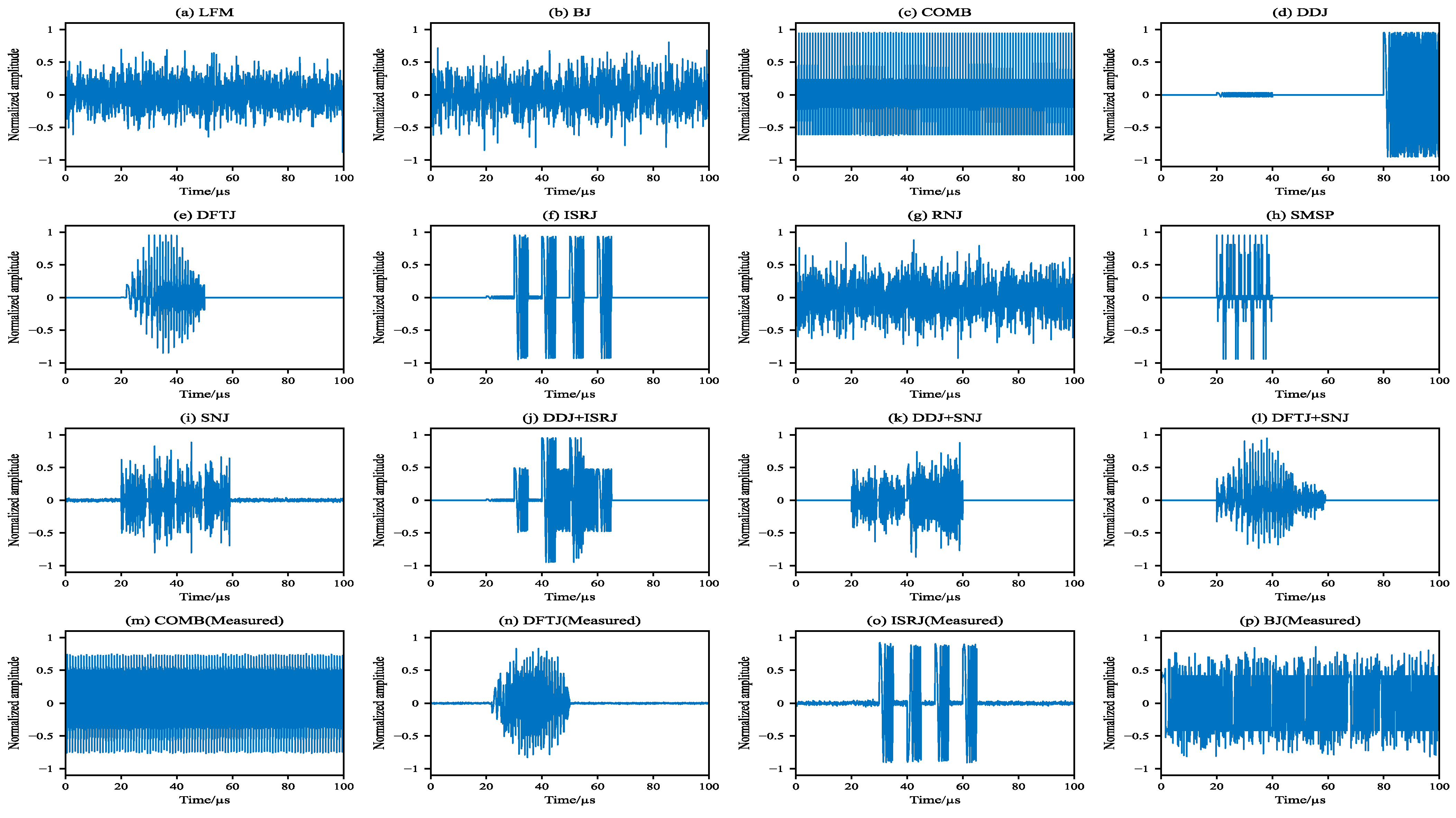
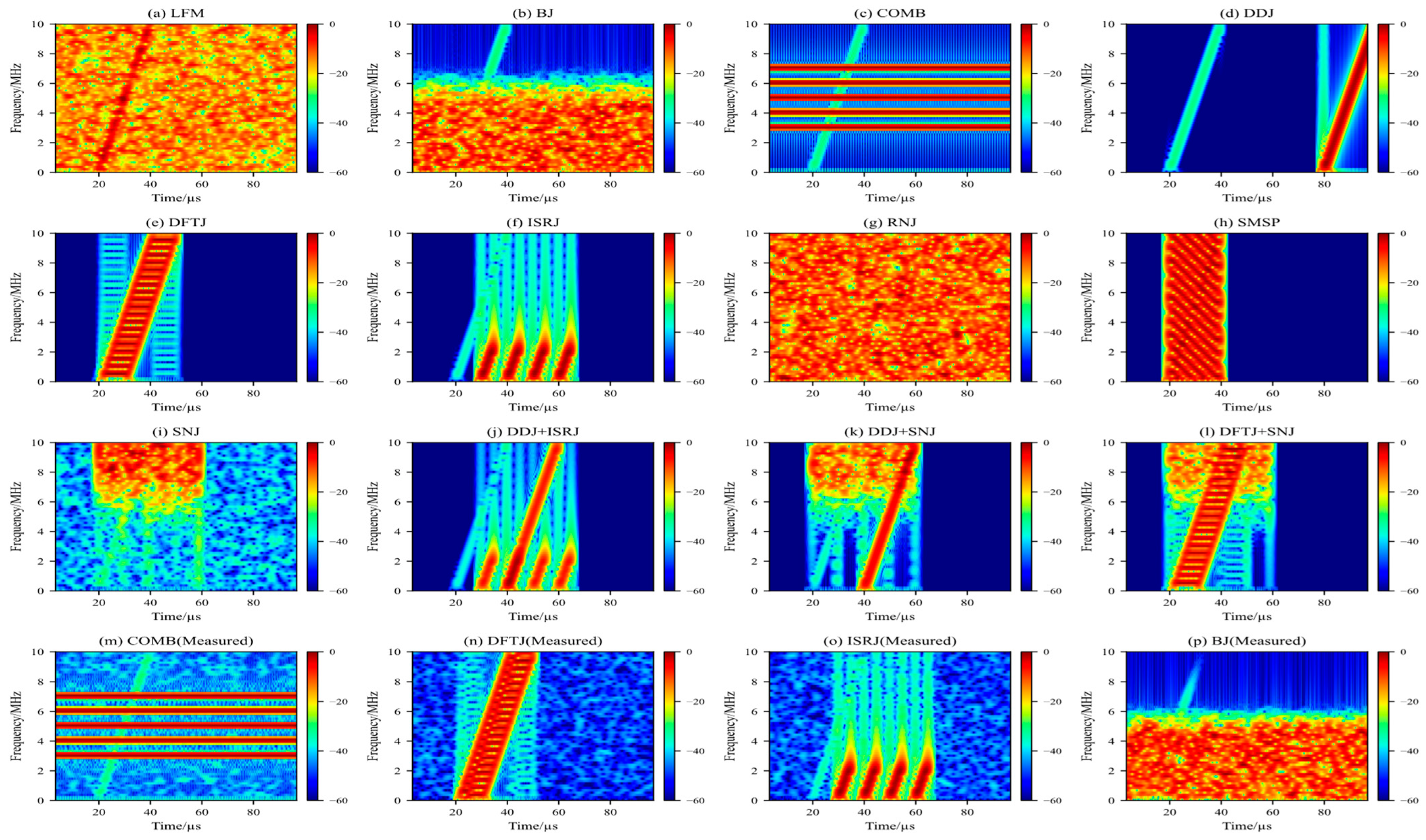
Figure 4 and Figure 5 present the time-domain waveforms and time–frequency spectrograms of representative signals, respectively. From these figures, the distinct differences in the time-domain characteristics and time–frequency distributions of different jamming types can be clearly observed.
Comparative experiments are conducted to evaluate the proposed algorithm against several representative radar jamming recognition methods. Furthermore, each method is trained using the same training parameters as in the original paper. Depending on various technical approaches, they are divided into three main types: traditional single-branch deep learning (1D-CNN-LSTM [47], LSTM [47]), enhanced convolutional neural network (WECNN [46], WECNN-TL [46]), and time–frequency domain joint inference model (JR-TFSAD [45]). Evaluation metrics are used to assess performance quantitatively in this work.

4.2. Evaluation Metrics

The OA, average accuracy (AA), recall, F1-score (F1), Kappa coefficient, Matthews correlation coefficient (MCC) [48,49], and mean average precision (mAP) [50,51] are used to measure the model’s recognition performance, and the model training time is also recorded as a metric which can show the computational complexity and engineering practicality of all compared algorithms. All quantitative results are presented in the form of mean ± standard deviation (std) to simultaneously evaluate the recognition accuracy and result stability of the model.
For subsequent indicator calculations, some parameters need to be defined. N is the total number of test set samples, K is the number of jamming classes, and the confusion matrix is C M N K × K , where C M i , j is the number of samples with ground-truth class i and predicted class j . The true positive for class c is defined as T P c = C M c , c . True positive (TP) counts samples that belong to category c and are correctly classified. The false positive for class c is defined as F P c = i = 1 , i c K   C M i , c , samples that do not belong to category c but are incorrectly labeled as c . False negative for class c is defined as F N c = j = 1 , j c K   C M c , j , samples from category c that are wrongly assigned to other classes, and true negative for class c is defined as T N c = N T P c F P c F N c , which covers samples outside category c that get a correct negative recognition, and the above evaluation metrics can be expressed as follows:
O A = 1 N c = 1 K   T P c
A A = 1 K c = 1 K   P r e c i s i o n c = 1 K c = 1 K   T P c T P c + F P c
R e c a l l = 1 K c = 1 K   R e c a l l c = 1 K c = 1 K   T P c T P c + F N c
F 1 = 1 K c = 1 K   F 1 c = 1 K c = 1 K   2 × P r e c i s i o n c × R e c a l l c P r e c i s i o n c + R e c a l l c
The Kappa coefficient is used to measure the consistency between model predictions and ground-truth labels. It also reduces the bias from random guesses in recognition results.
K a p p a = p o p e 1 p e
where p o is the observed recognition consistency, and p e denotes the expected consistency from random recognition. Then the calculation formula of p e is
p e = ( a 1 × b 1 + a 2 × b 2 + + a K × b K ) N 2
M C C = N c = 1 K   T P c c = 1 K   a c b c N 2 ( c = 1 K   a c ) 2 N 2 ( c = 1 K   b c ) 2
where a c = T P c + F N c represents the total number of samples of class c , and b c = T P c + F P c represents the total number of samples predicted as class c .
m A P = 1 K c = 1 K   ( A U C ( R e c a l l c , P r e c i s i o n c ) )
To evaluate the effectiveness of the proposed method, the complete dataset was divided into mutually exclusive training, validation, and test subsets. The dataset consists of 16 categories, and each category contains 500 independent samples. For few-shot evaluation, 3%, 5%, 7%, 9%, and 11% of the samples from each category were selected without replacement to construct the corresponding training subsets, corresponding to 15, 25, 35, 45, and 55 training samples per category, respectively. During model optimization, a validation subset was further generated from the training data using stratified sampling for model selection and early stopping. All remaining samples were used for testing. The training, validation, and test subsets were mutually exclusive to avoid potential information leakage during evaluation. This experimental setup simulates the low-sample scenarios commonly encountered in practical radar operations. In addition, all experiments under different training ratios were independently repeated 10 times to reduce the influence of randomness and ensure the reliability of the reported results.

4.3. Experimental Configuration

Table 3 lists all training parameters for ACDF-Net model. For all compared methods, the original training configurations from their published references were strictly followed. This ensures complete fairness in all comparison experiments.
All simulation data in this work are generated in the MATLAB 2020b environment. All recognition tests are performed on a workstation with a 2.2 GHz CPU, 64.0 GB of RAM, and an RTX 4090 GPU. All code is written in 64-bit Python 3.11.

4.4. Experimental Results

Comparative experiments, per-class performance analysis, model stability validation, and ablation studies were conducted to verify the performance of the proposed ACDF-Net. The quantitative results are summarized in Table 4, Table 5, Table 6 and Table 7, and visualization results are shown in Figure 6, Figure 7, Figure 8, Figure 9, Figure 10, Figure 11 and Figure 12. Table 5 summarizes the ablation results under the 3% training setting, including single-branch baselines, feature concatenation, fixed fusion, and the proposed ACDF-Net. Multiple evaluation metrics were used to comprehensively evaluate classification performance and efficiency under few-shot conditions.
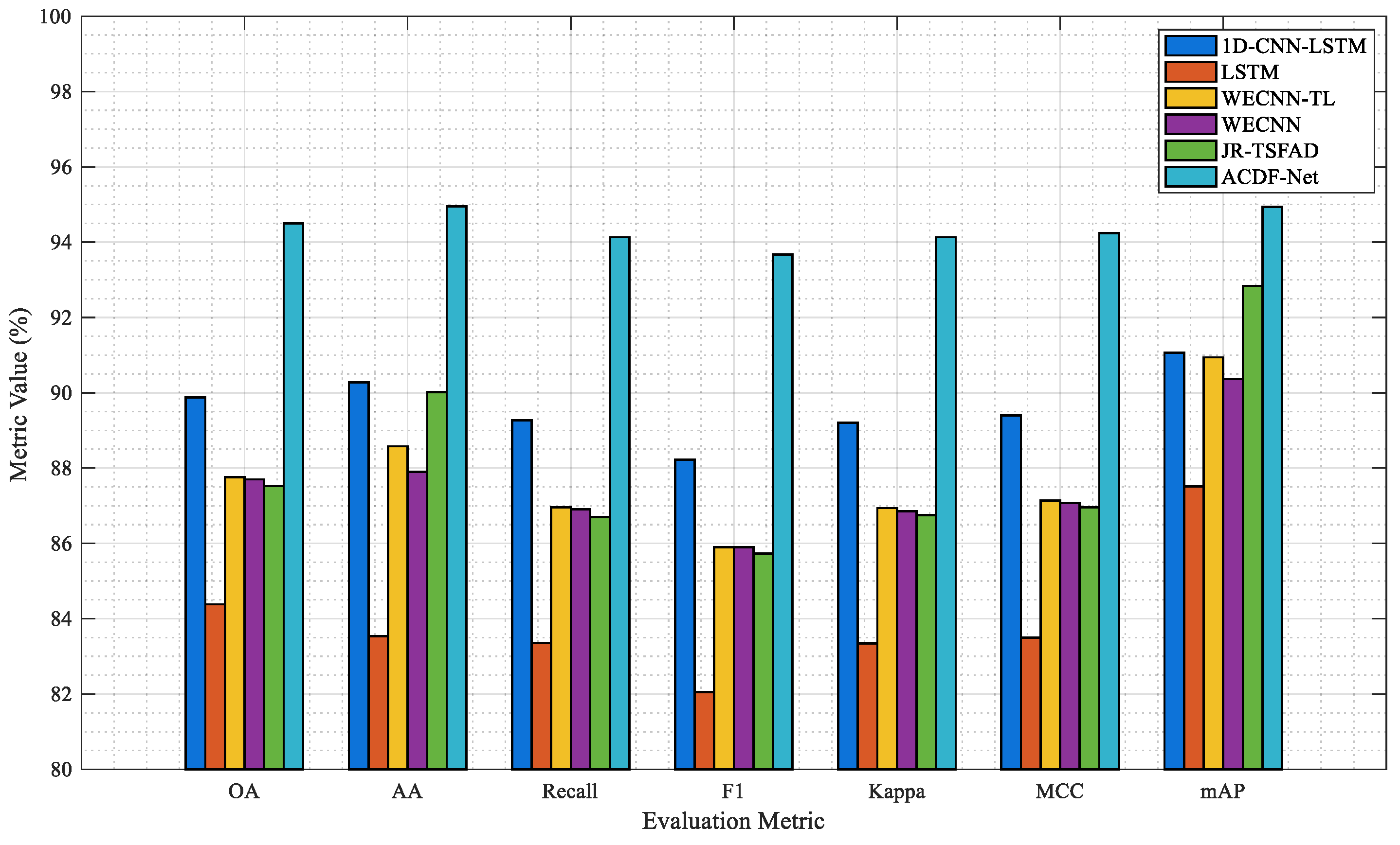
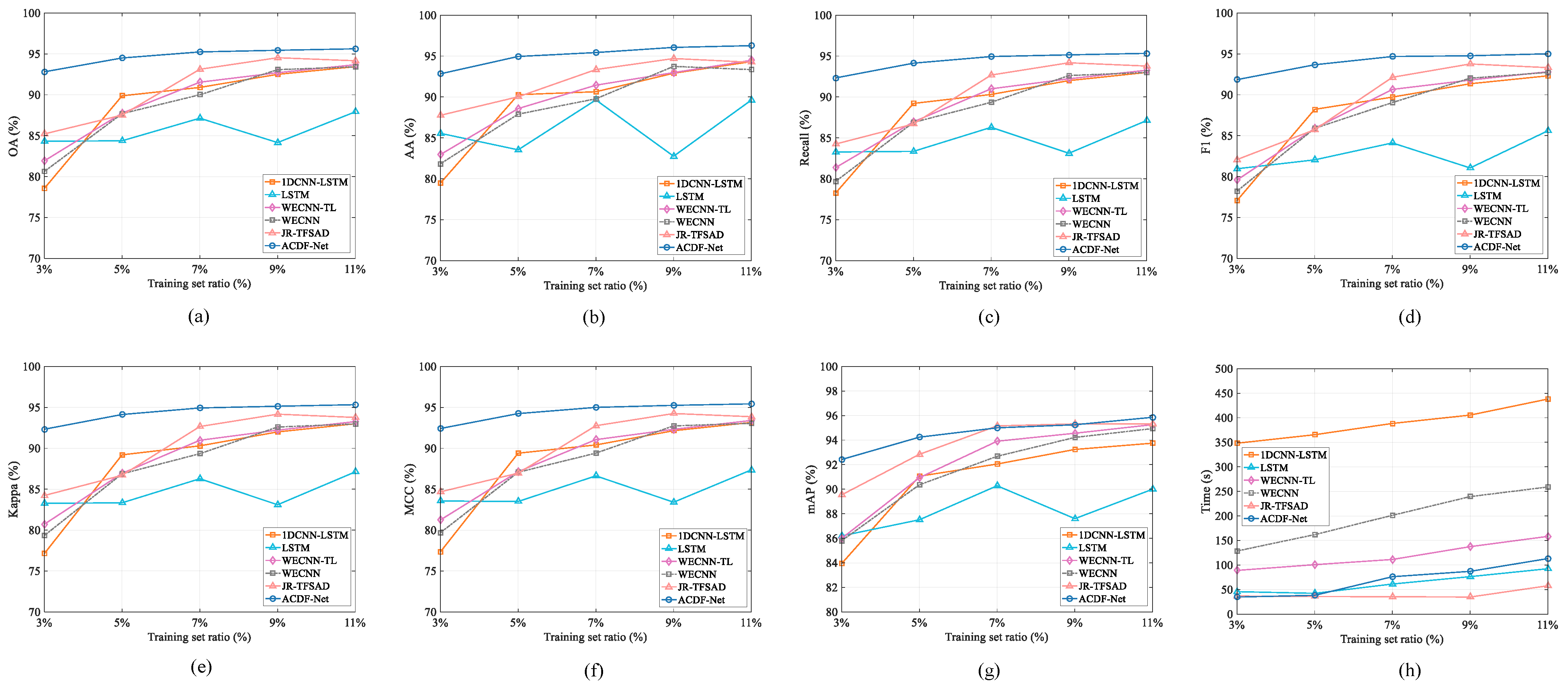
The performance across multiple metrics using a 5% training set is shown in Figure 6, which demonstrates ACDF-Net’s performance advantages over all comparison algorithms. Figure 7 shows the performance trends of all methods across training set sizes ranging from 3% to 11%. As the number of training samples increases, all recognition metrics show an upward trend, because more training data allows the model to learn more features. ACDF-Net completes training on a 3% training set in just 34.78 s, which is 5.5% faster than the lightweight JR-TFSAD and 90.0% faster than the complex 1D-CNN-LSTM model. Even when using a 5% training set, its training time is only 38.28 s, achieving a better balance between recognition accuracy and computational efficiency.
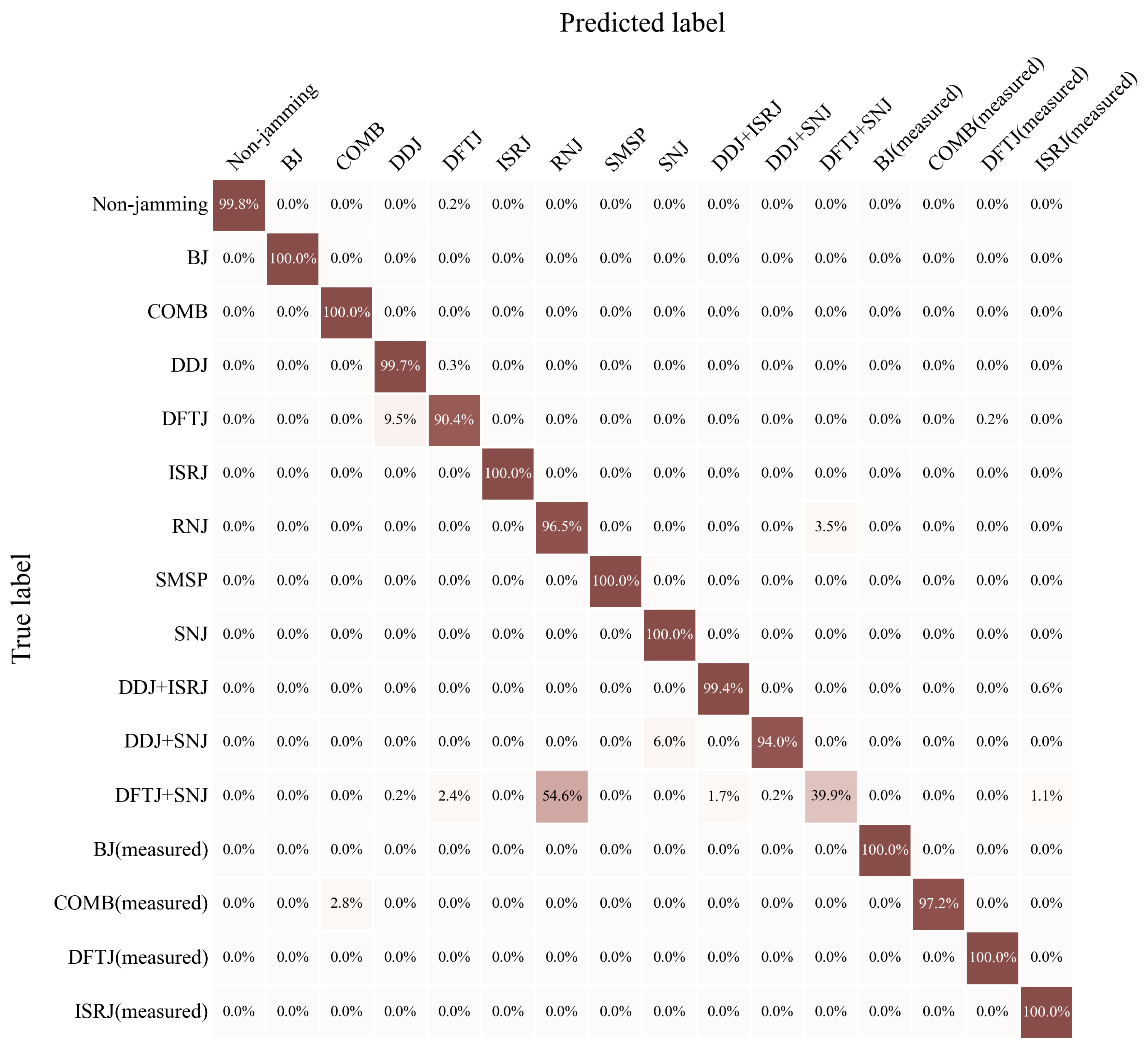
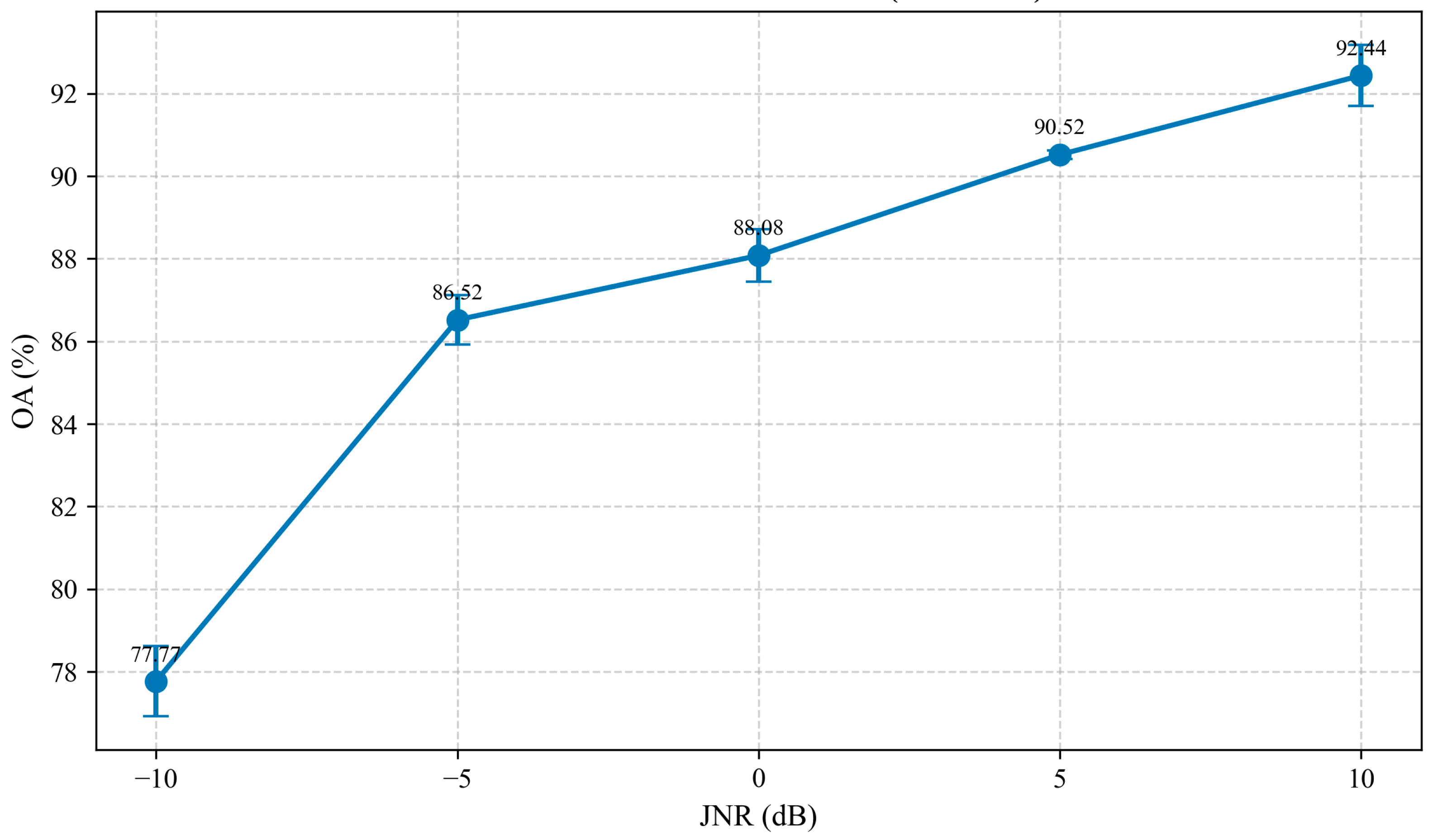
Figure 8 presents the confusion matrix of ACDF-Net under the 5% few-shot training setting. The matrix is normalized by rows, and the diagonal values represent the recall of each jamming category. Most categories achieve satisfactory recognition performance, including BJ, COMB, ISRJ, SMSP, SNJ, BJ (measured), DFTJ (measured), and ISRJ (measured), which obtain recognition rates close to or equal to 100%. The main classification errors occur among spectrally similar composite interference types. In particular, DFTJ + SNJ is the most challenging category, with only 39.9% recall and 54.6% of samples misclassified as RNJ due to their similar energy distribution and modulation characteristics. These results indicate that ACDF-Net effectively distinguishes most jamming categories while revealing the remaining challenges in recognizing highly similar composite interference patterns. To further evaluate the robustness of ACDF-Net under challenging interference conditions, experiments were conducted under low-JNR scenarios. The JNR was varied from −10 dB to 10 dB while maintaining the 5% training set setting. As shown in Figure 9, the recognition performance gradually improves with increasing JNR. Notably, ACDF-Net still achieves an OA of 77.77% at −10 dB JNR, demonstrating its capability to extract discriminative features under severe interference conditions.
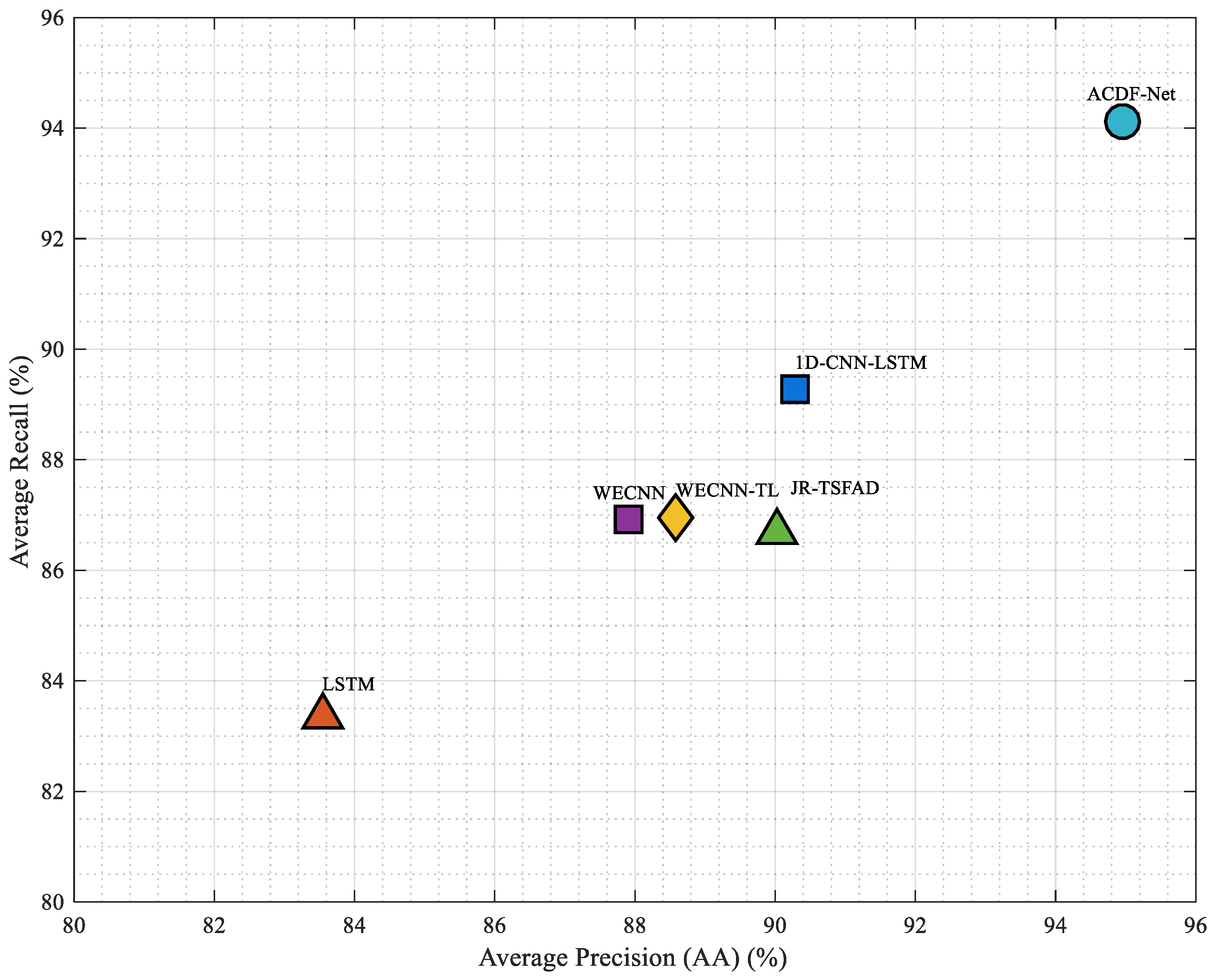
Figure 10 shows the precision–recall balance curves for each algorithm. ACDF-Net is located in the upper-right corner of the figure, exhibiting the highest average precision and average recall among all methods. It achieves the optimal balance between precision and recall.
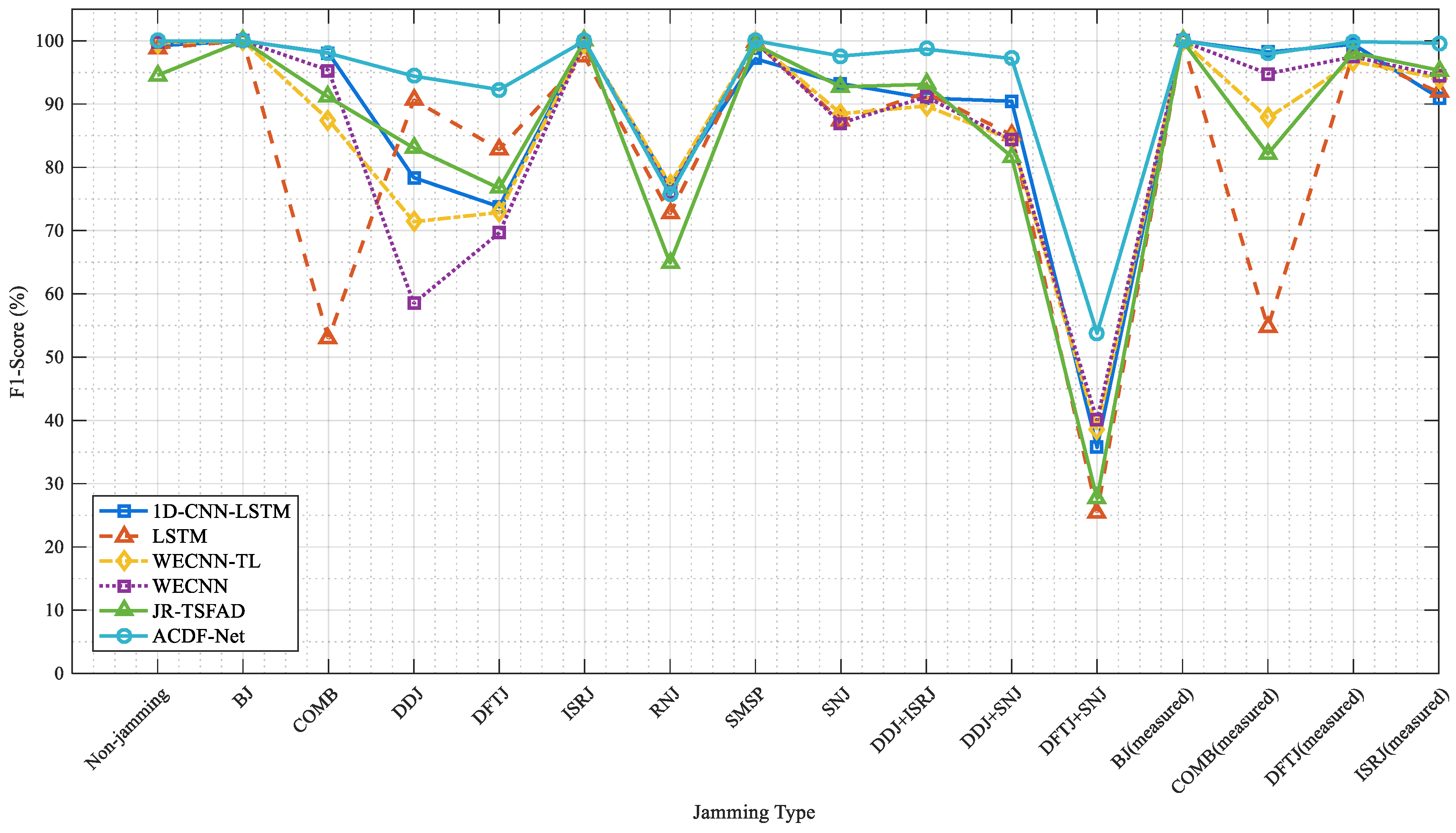
For distinguishable single jamming types (such as BJ and SMSP), the recognition accuracy of all algorithms exceeds 99%. For low-distinguishability jamming, composite jamming, and non-ideal measurement jamming signals, the performance of traditional methods drops significantly, whereas ACDF-Net maintains strong robustness; the AA of the proposed method on COMB jamming reaches 96.19%, which is 41.4 percentage points higher than that of the baseline LSTM model. The AA for all types of measurement jamming exceeds 99%, and among the 16 signal categories, 14 maintain an average accuracy of ≥88%, as shown by the F1 comparison in Figure 11.
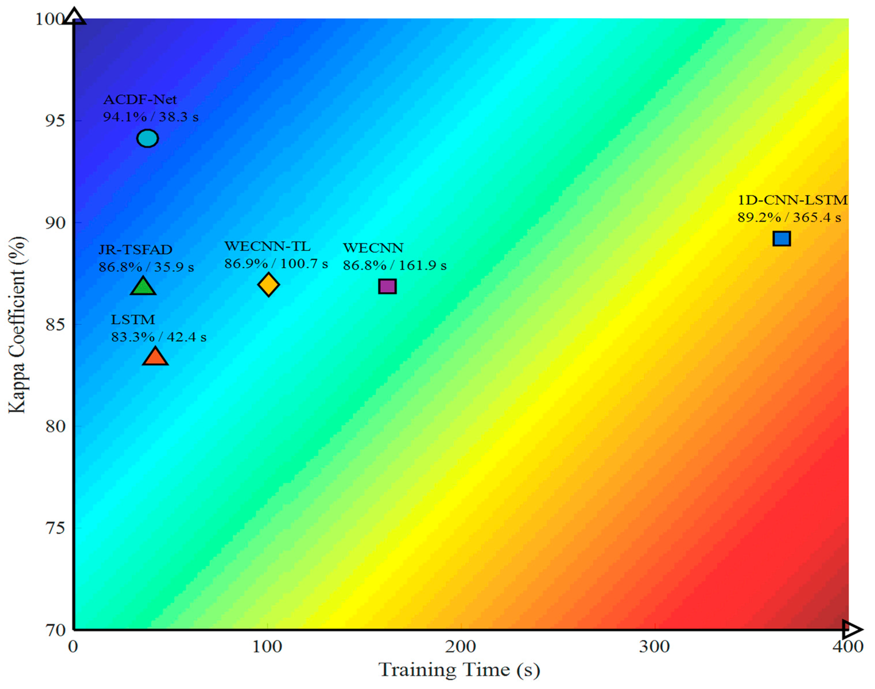
Figure 12 quantifies the trade-off between the model’s recognition performance (Kappa coefficient) and computational cost (training time). ACDF-Net is located in the blue optimal region in the upper-left corner of the chart, achieving a Kappa coefficient of 94.1% within a training time of 38.3 s. It achieves a favorable balance of performance and efficiency among all compared algorithms, highlighting its practical value for engineering applications.
Ablation experiments using training set sizes of 3% and 5% were conducted to verify the effectiveness of ACDF-Net’s core components, and the results are shown in Table 8 and Table 9 (3% and 5% training ratios, respectively).
Table 8 and Table 9 present the ablation study results under 3% and 5% training set settings to evaluate the contribution of each component in the proposed framework. The configurations include removing the dual-branch representation, removing the adaptive fusion strategy, their combination, and comparisons with baseline methods.
The results show that removing the dual-branch structure leads to significant performance drops of 8.93% and 3.61% in OA under 3% and 5% settings, respectively, indicating its effectiveness in learning complementary representations. When the adaptive fusion strategy is removed under the dual-branch setting, OA decreases by 3.00% and 0.08%, respectively, demonstrating its stronger impact under few-shot conditions. In addition, the learned fusion weights (α) are statistically stable across different training ratios, with mean values of 0.572 ± 0.048 (3%) and 0.528 ± 0.031 (5%), indicating that the model can automatically adaptively balance the contributions of the two branches without manual tuning. Furthermore, per-class performance observations indicate that most categories are correctly classified, while errors mainly occur among visually similar jamming types under extremely limited training samples. This further demonstrates the improved feature separability achieved by the proposed dual-branch fusion framework.
Overall, the dual-branch representation and adaptive fusion strategy exhibit a clear synergistic effect, achieving up to 7.10% OA improvement with moderate computational overhead, confirming the effectiveness of each component, especially under few-shot conditions.
Nevertheless, the proposed method still has limitations. For composite jamming signal (DFTJ + SNJ) and the single jamming signal RNJ, the algorithm’s recognition accuracy does not achieve significant improvement; when processing a small number of samples, the standard deviation of the recognition results is slightly higher than that of the comparison algorithm.

5. Conclusions

In complex electromagnetic environments, active radar jamming recognition faces two key challenges: it is difficult to obtain large-scale jamming samples in non-cooperative confrontation scenarios, and traditional methods perform poorly in few-shot scenarios. To address these issues, we propose a novel Adaptive Confidence Dual-Branch Fusion Network (ACDF-Net) for few-shot radar jamming recognition. This model utilizes four-channel time–frequency information to preserve modulation information of the jamming signal, and employs a dual-branch architecture to learn modulation features and energy-phase features separately. It combines learnable adaptive confidence fusion to optimize recognition results. Experiments conducted on the constructed dataset (which includes both synthetic and real jamming signals) demonstrate that, when trained on 3% of the training samples, ACDF-Net achieves an OA of 92.81% and a mAP of 93.56%, outperforming selected models in few-shot scenarios. ACDF-Net maintains stable recognition performance on real jamming signals. Ablation experiments confirm that the dual-branch complementary representation structure and the adaptive confidence fusion module are the core factors driving the performance improvement in few-shot scenarios. However, the proposed method still has significant limitations. On the one hand, for low-discriminability jamming, such as RNJ and DFTJ + SNJ, the recognition rate remains low with no significant improvement achieved. On the other hand, the recognition stability across different categories is insufficient, and the model does not have the generalization ability to identify unseen jamming types. Future work will focus on the targeted optimization of the proposed model to mitigate the above limitations, and advance its translation to practical engineering applications in complex electromagnetic environments.

Author Contributions

Conceptualization, B.C. and Q.L.; methodology, B.C. and Q.L.; software, B.C.; validation, B.C. and Q.L.; formal analysis, B.C.; investigation, B.C.; resources, Q.L.; data curation, B.C.; writing—original draft preparation, B.C.; writing—review and editing, Q.L. and M.L.; visualization, B.C.; supervision, Q.L.; project administration, Q.L.; funding acquisition, Q.L. All authors have read and agreed to the published version of the manuscript.

Funding

This research was supported by Guangxi Key Technologies R&D Program (No. GuikeFN2600640466), Guangxi Key Technologies R&D Program (No. GuikeAB23026147), Guangxi Science and Technology Major Program (No. GuikeAA23023010), and Guangxi Baise Scientific Research and Technology Development Plan Project (No. Baike202432012).

Data Availability Statement

The code and data are available from the corresponding author.

Conflicts of Interest

The authors declare no conflicts of interest.

References

  1. Chen, Y.; Wang, Y.; Qu, F.; Li, W. A graph-based track-before-detect algorithm for automotive radar target detection. IEEE Sens. J. 2021, 21, 6587–6599. [Google Scholar] [CrossRef]
  2. Du, L.; Li, L.; Wei, D.; Mao, J. Saliency-guided single shot multibox detector for target detection in SAR images. IEEE Trans. Geosci. Remote Sens. 2020, 58, 3366–3376. [Google Scholar] [CrossRef]
  3. Tan, M.; Wang, C.; Xue, B.; Xu, J. A novel deceptive jamming approach against frequency diverse array radar. IEEE Sens. J. 2021, 21, 8323–8332. [Google Scholar] [CrossRef]
  4. Du, C.; Zhao, Y.; Wang, L.; Tang, B.; Xiong, Y. Deceptive multiple false targets jamming recognition for linear frequency modulation radars. J. Eng. 2019, 21, 7690–7694. [Google Scholar] [CrossRef]
  5. Wang, W.; Wu, J.; Pei, J.; Sun, Z.; Yang, J.; Yi, Q. Antirange-deceptive jamming from multijammer for multistatic SAR. IEEE Trans. Geosci. Remote Sens. 2022, 60, 5212512. [Google Scholar] [CrossRef]
  6. Ali, M.A.; Ahmed, H.; Saadia, R.; Ahmed, W.; Tahir, F. Electronic deceptive jamming: False target generation in radars. In Proceedings of the International Conference on Recent Advances in Electrical Engineering and Computer Sciences (RAEECS), Islamabad, Pakistan, 18–20 October 2022; pp. 1–6. [Google Scholar]
  7. Iqbal, Y.; Jawad, M. An effective coherent noise jamming method for deception of wideband LFM radars. In Proceedings of the 17th International Bhurban Conference on Applied Sciences and Technology (IBCAST), Islamabad, Pakistan, 14–18 January 2020; pp. 622–626. [Google Scholar]
  8. Lou, M.; Yang, J.; Li, Z.; Ren, H.; An, H.; Wu, J. Joint optimal and adaptive 2-D spatial filtering technique for FDA-MIMO SAR deceptive jamming separation and suppression. IEEE Trans. Geosci. Remote Sens. 2022, 60, 5238414. [Google Scholar] [CrossRef]
  9. Orlando, D. A novel noise jamming detection algorithm for radar applications. IEEE Signal Process. Lett. 2017, 24, 206–210. [Google Scholar] [CrossRef]
  10. Zhang, S.; Zhou, Y.; Zhang, L.; Zhang, Q.; Du, L. Target detection for multi static radar in the presence of deceptive jamming. IEEE Sens. J. 2021, 21, 8130–8141. [Google Scholar] [CrossRef]
  11. Luo, Z.; Cao, Y.; Yeo, T.-S.; Wang, F. Few-shot radar jamming recognition network via complete information mining. IEEE Trans. Aerosp. Electron. Syst. 2024, 60, 3625–3638. [Google Scholar] [CrossRef]
  12. Zhou, H.; Dong, C.; Wu, R.; Xu, X.; Guo, Z. Feature fusion based on Bayesian decision theory for radar deceptive jamming recognition. IEEE Access 2021, 9, 16296–16304. [Google Scholar] [CrossRef]
  13. Sun, D.; Li, A.; Ding, H.; Wei, J. Detection of DRFM deceptive jamming based on diagonal integral bispectrum. Remote Sens. 2025, 17, 1957. [Google Scholar] [CrossRef]
  14. Wu, W.; Zou, J.; Chen, J.; Xu, S.; Chen, Z. False-target recognition against interrupted-sampling repeater jamming based on integration decomposition. IEEE Trans. Aerosp. Electron. Syst. 2021, 57, 2979–2991. [Google Scholar] [CrossRef]
  15. Xu, Z.; Shi, Q.; Shi, J.; Wang, H.; Wei, M.; Gao, R.; Shao, Y.; Tao, H. A Novel Method of Mitigating the Mutual Interference between Multiple LFMCW Radars for Automotive Applications. In IGARSS 2019—2019 IEEE International Geoscience and Remote Sensing Symposium; IEEE: Piscataway, NJ, USA, 2019. [Google Scholar] [CrossRef]
  16. Xu, Z.; Shi, Q. Interference Mitigation for Automotive Radar Using Orthogonal Noise Waveforms. IEEE Geosci. Remote Sens. Lett. 2018, 15, 137–141. [Google Scholar] [CrossRef]
  17. Xu, Z.; Wang, X.; Wang, Y. Nonlinear Frequency-Modulated Waveforms Modeling and Optimization for Radar Applications. Mathematics 2022, 10, 3939. [Google Scholar] [CrossRef]
  18. Greco, M.; Gini, F.; Farina, A. Radar detection and classification of jamming signals belonging to a cone class. IEEE Trans. Signal Process. 2008, 56, 1984–1993. [Google Scholar] [CrossRef]
  19. Xing, H.; Xing, Q.; Wang, K. Radar anti-jamming countermeasures intelligent decision-making: A partially observable Markov decision process approach. Aerospace 2023, 10, 236. [Google Scholar] [CrossRef]
  20. Bandiera, F.; Farina, A.; Orlando, D.; Ricci, G. Detection algorithms to discriminate between radar targets and ECM signals. IEEE Trans. Signal Process. 2010, 58, 5984–5993. [Google Scholar] [CrossRef]
  21. Zhao, S.; Zhou, Y.; Zhang, L.; Guo, Y.; Tang, S. Discrimination between radar targets and deceptive jamming in distributed multiple-radar architectures. IET Radar Sonar Navig. 2017, 11, 1124–1131. [Google Scholar] [CrossRef]
  22. Su, D.; Gao, M. Research on jamming recognition technology based on characteristic parameters. In Proceedings of the IEEE 5th International Conference on Signal and Image Processing, Beijing, China, 23–25 October 2020; pp. 303–307. [Google Scholar]
  23. Hao, Z.; Yu, W.; Chen, W. Recognition method of dense false targets jamming based on time-frequency atomic decomposition. J. Eng. 2019, 2019, 6354–6358. [Google Scholar] [CrossRef]
  24. Xu, Z.; Xue, S.; Wang, Y. Incoherent Interference Detection and Mitigation for Millimeter-Wave FMCW Radars. Remote Sens. 2022, 14, 4817. [Google Scholar] [CrossRef]
  25. Xu, Z. Bi-level l1 optimization-based interference reduction for millimeter wave radars. IEEE Trans. Intell. Transp. Syst. 2023, 24, 728–738. [Google Scholar] [CrossRef]
  26. Xu, Z.; Yuan, M. An Interference Mitigation Technique for Automotive Millimeter Wave Radars in the Tunable Q-Factor Wavelet Transform Domain. IEEE Trans. Microw. Theory Tech. 2021, 69, 5270–5283. [Google Scholar] [CrossRef]
  27. Wu, Z.; Zhang, Y. A hybrid 1D-2D CNN with decision-level fusion for radar active deceptive jamming recognition. In Proceedings of the 7th International Conference on Information Science, Electrical and Automation Engineering (ISEAE), Harbin, China, 18–20 April 2025; pp. 668–672. [Google Scholar] [CrossRef]
  28. Xu, H.; Quan, Y.; Zhou, X.; Chen, H.; Cui, T.J. A novel approach for radar passive jamming based on multiphase coding rapid modulation. IEEE Trans. Geosci. Remote Sens. 2023, 61, 5101614. [Google Scholar] [CrossRef]
  29. Liu, Q.; Zhang, W. Deep learning and recognition of radar jamming based on CNN. In Proceedings of the 12th International Symposium on Computational Intelligence and Design (ISCID), Hangzhou, China, 14–15 December 2019; pp. 208–212. [Google Scholar] [CrossRef]
  30. Cai, Y.; Shi, K.; Song, F.; Xu, Y.; Wang, X.; Luan, H. Jamming pattern recognition using spectrum waterfall: A deep learning method. In Proceedings of the IEEE 5th International Conference on Computer and Communications (ICCC), Chengdu, China, 6–9 December 2019; pp. 2113–2117. [Google Scholar] [CrossRef]
  31. Du, L.; Li, F.; He, X.; Li, Y. Radar deceptive jamming recognition based on multi-dimensional feature extraction. In Proceedings of the IEEE International Conference on Signal, Information and Data Processing (ICSIDP), Zhuhai, China, 22–24 November 2024; pp. 1–6. [Google Scholar] [CrossRef]
  32. Cheng, L.; Cao, S. TransRAD: Retentive Vision Transformer for Enhanced Radar Object Detection. IEEE Trans. Radar Syst. 2025, 3, 303–317. [Google Scholar] [CrossRef]
  33. Cheng, L.; Sengupta, A.; Cao, S. 3D Radar and Camera Co-Calibration: A Flexible and Accurate Method for Target-Based Ex-trinsic Calibration. In Proceedings of the 2023 IEEE Radar Conference (RadarConf23), San Antonio, TX, USA, 8–11 May 2023; pp. 1–6. [Google Scholar] [CrossRef]
  34. Lu, J.; Guo, Y.; Feng, W.; Hu, X.; Gong, J.; Zhang, Y. Intelligent Recognition and Parameter Estimation of Radar Active Jamming Based on Oriented Object Detection. Remote Sens. 2025, 17, 2646. [Google Scholar] [CrossRef]
  35. Kong, Y.; Wang, X.; Wu, C.; Yu, X.; Cui, G. Active deceptive jamming recognition in the presence of extended target. IEEE Geosci. Remote Sens. Lett. 2022, 19, 4024905. [Google Scholar] [CrossRef]
  36. Hou, L.; Zhang, S.; Wang, C.; Li, X.; Chen, S.; Zhu, L.; Zhu, Y. Jamming recognition of carrier-free UWB cognitive radar based on MANet. IEEE Trans. Instrum. Meas. 2023, 72, 8504413. [Google Scholar] [CrossRef]
  37. Chen, H.; Chen, H.; Lei, Z.; Zhang, L.; Li, B.; Zhang, J.; Wang, Y. Compound Jamming Recognition Based on a Dual-Channel Neural Network and Feature Fusion. Remote Sens. 2024, 16, 1325. [Google Scholar] [CrossRef]
  38. Chen, X.; Liu, Y.; Wang, C. Multi-Domain Fusion Network for Active Jamming Recognition in Cognitive Radar. Remote Sens. 2025, 17, 1723. [Google Scholar] [CrossRef]
  39. Li, L.; Huang, L.; Meng, T.; Xing, C.; Yang, T.; Li, W.; Lu, P. MFE-STN: A Versatile Front-End Module for SAR Deception Jamming False Target Recognition. Remote Sens. 2025, 17, 3848. [Google Scholar] [CrossRef]
  40. Qian, J.; Teng, X.; Qiu, Z. Recognition of radar deceptive jamming based on convolutional neural network. IET Conf. Proc. 2021, 2020, 913–918. [Google Scholar] [CrossRef]
  41. Cao, X. Few-shot and zero-shot radar active jamming recognition based on a vision-language model. IEEE Trans. Aerosp. Electron. Syst. 2025, 61, 14795–14808. [Google Scholar] [CrossRef]
  42. Luo, J.; Si, W.; Deng, Z. Few-shot learning for radar signal recognition based on tensor imprint and re-parameterization multi-channel multi-branch model. IEEE Signal Process. Lett. 2022, 29, 1327–1331. [Google Scholar] [CrossRef]
  43. Wu, Z.; Wang, T.; Cao, Y.; Zhang, M.; Guo, W.; Yang, L. Few-shot radar active jamming recognition under label prior information reuse. IEEE Geosci. Remote Sens. Lett. 2025, 22, 3501305. [Google Scholar] [CrossRef]
  44. Lin, Z.; Ji, K.; Kang, M.; Leng, X.; Zou, H. Deep convolutional highway unit network for SAR target classification with limited labeled training data. IEEE Geosci. Remote Sens. Lett. 2017, 14, 1091–1095. [Google Scholar] [CrossRef]
  45. Luo, Z.; Cao, Y.; Yeo, T.-S.; Wang, Y.; Wang, F. Few-shot radar jamming recognition network via time-frequency self-attention and global knowledge distillation. IEEE Trans. Geosci. Remote Sens. 2023, 61, 5105612. [Google Scholar] [CrossRef]
  46. Lv, Q.; Quan, Y.; Feng, W.; Sha, M.; Dong, S.; Xing, M. Radar deceptive jamming recognition based on weighted ensemble CNN with transfer learning. IEEE Trans. Geosci. Remote Sens. 2022, 60, 5107511. [Google Scholar] [CrossRef]
  47. Feng, X.; Zhang, X.; He, K.; Tan, P.; Tang, Y. A multiclass time-series signal recognition method based on a large active radar jamming database. IEEE Sens. J. 2025, 25, 20051–20066. [Google Scholar] [CrossRef]
  48. Matthews, B.W. Comparison of the predicted and observed secondary structure of T4 phage lysozyme. Biochim. Biophys. Acta 1975, 405, 442–451. [Google Scholar] [CrossRef] [PubMed]
  49. Chicco, D.; Jurman, G. The advantages of the Matthews correlation coefficient (MCC) over F1 score and accuracy in binary classification evaluation. BMC Genom. 2020, 21, 6. [Google Scholar] [CrossRef] [PubMed]
  50. Everingham, M.; Van Gool, L.; Williams, C.K.I.; Winn, J.; Zisserman, A. The PASCAL visual object classes (VOC) challenge. Int. J. Comput. Vis. 2010, 88, 303–338. [Google Scholar] [CrossRef]
  51. Peng, R.; Wu, X.; Wang, Z.L.H. Intelligent recognition and information extraction of radar complex jamming based on time-frequency features. J. Syst. Eng. Electron. 2024, 35, 1148–1166. [Google Scholar] [CrossRef]
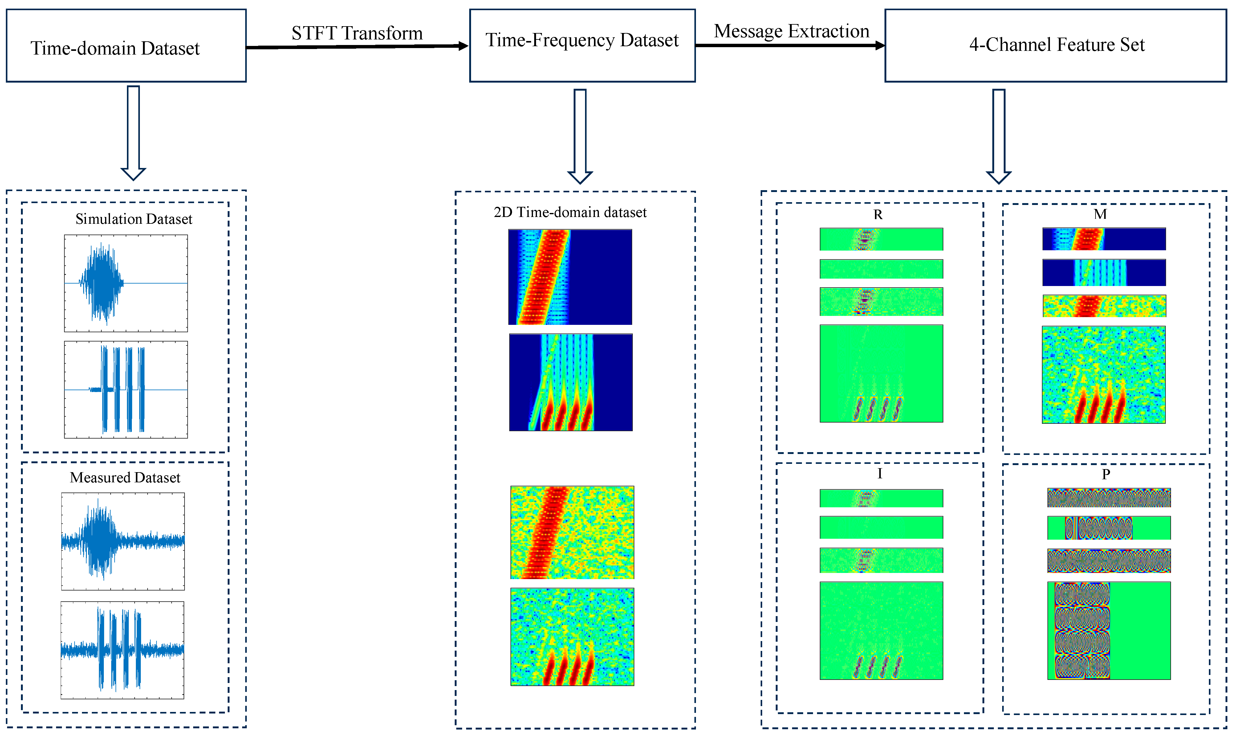
Figure 1. Flowchart of radar jamming signal preprocessing.
Electronics 15 03576 g001
Figure 2. Overall architecture of the proposed ACDF-Net for few-shot radar signal recognition.
Electronics 15 03576 g002
Figure 3. Structure of the basic residual block.
Electronics 15 03576 g003
Figure 4. Time-domain waveforms of the above radar jamming signals: (a) LFM (non-jamming); (b) BJ; (c) COMB; (d) DDJ; (e) DFTJ; (f) ISRJ; (g) RNJ; (h) SMSP; (i) SNJ; (j) DDJ + ISRJ; (k) DDJ + SNJ; (l) DFTJ + SNJ; (m) COMB (measured); (n) DFTJ (measured); (o) ISRJ (measured); (p) BJ (measured).
Electronics 15 03576 g004
Figure 5. Time–frequency spectrograms of the above radar jamming signals: (a) LFM (non-jamming); (b) BJ; (c) COMB; (d) DDJ; (e) DFTJ; (f) ISRJ; (g) RNJ; (h) SMSP; (i) SNJ; (j) DDJ + ISRJ; (k) DDJ + SNJ; (l) DFTJ + SNJ; (m) COMB (measured); (n) DFTJ (measured); (o) ISRJ (measured); (p) BJ (measured).
Electronics 15 03576 g005
Figure 6. Multi-index comprehensive performance comparison (training set: 5%).
Electronics 15 03576 g006
Figure 7. Evolution of the evaluation metrics according to the training set size: (a) OA; (b) AA; (c) recall; (d) F1; (e) Kappa; (f) MCC; (g) mAP; (h) training time.
Electronics 15 03576 g007
Figure 8. A confusion matrix of ACDF-Net (training set: 5%).
Electronics 15 03576 g008
Figure 9. OA of the proposed ACDF-Net under different JNRs (training set: 5%).
Electronics 15 03576 g009
Figure 10. Precision–recall balance of different algorithms (training set: 5%).
Electronics 15 03576 g010
Figure 11. F1 Comparison of all jamming types (training set: 5%).
Electronics 15 03576 g011
Figure 12. Evaluating model performance: simultaneously using the Kappa coefficient and the time cost.
Electronics 15 03576 g012
Table 1. Architecture of the proposed dual-branch ResNet18 backbone.
LayerConv. KernelActivationMaxPoolDropoutOutput Size
Input- -- 2 × 100 × 247
Conv.1 ( 7 × 7 ) × 64 BN + ReLU 3 × 3 , s t r i d e = 2 - 64 × 25 × 62
ResBlock1 ( 3 × 3 ) × 64 × 2 ReLU-- 64 × 25 × 62
ResBlock2 ( 3 × 3 ) × 128 × 2
+ ( 1 × 1 ) × 128
ReLU-- 128 × 13 × 31
ResBlock3 ( 3 × 3 ) × 256 × 2
+ ( 1 × 1 ) × 256
ReLU-- 256 × 7 × 16
ResBlock4 ( 3 × 3 ) × 512 × 2
+ ( 1 × 1 ) × 512
ReLU-- 512 × 4 × 8
GAP- -- 1 × 512
Dropout---0.35 1 × 512
FC 512 16 --- 1 × 16
Output (Softmax)- -- 1 × 16
Table 2. Parameters of radar jamming signals in dataset.
SignalParametersRange of Values
LFM (non-jamming)Time width
Bandwidth
Sampling frequency
20 μ s
10 MHz
20 MHz
BJBase noise
Bandwidth
Gaussian noise (0, 1)
5 MHz–10 MHz
COMBComb num
Comb magnitude
Comb frequency step
3~5
0~1
1 MHz
DDJDelay in false target1~10 μ s
DFTJNum of false targets
Delay of false target
3~6
1~10 μ s
ISRJNum of forwarding times
Slice cycle
Duty cycle of sampling pulse
4
12.5 μ s
0.4~0.6
RNJBase noise
Attenuation factor
Gaussian noise (0, 1)
2~3
SMSPSampling factor3~5
SNJNum of forwarding times
Slice cycle
Duty cycle of sampling pulse
2~5
5~15 μ s
0.1~0.7
DDJ + ISRJ
DDJ + SNJ
DFTJ + SNJ
Num of forwarding times
Slice cycle
Duty cycle of sampling pulse num of false targets
Delay of false target
Determined by
specific jamming
Table 3. Training hyperparameters of ACDF-Net.
HyperparametersValues
Batch_size16
Epochs60
OptimizerAdamW
Label_smoothing0.12
Initial learning rate1 × 10−4
Weight decay1 × 10−5
Table 4. Results of the comparative experiment (training set size: 3% of the dataset).
Training: 3%1D-CNN-LSTMLSTMWECNN-TLWECNNJR-TFSADACDF-Net
OA (%)78.56 ± 0.4584.32 ± 0.8781.93 ± 0.8780.63 ± 0.8685.22 ± 2.9192.81 ± 0.62
AA (%)79.47 ± 1.5885.56 ± 1.8282.96 ± 0.7881.83 ± 1.2687.76 ± 1.5892.83 ± 1.23
Recall (%)78.26 ± 1.8583.28 ± 0.9581.37 ± 0.0379.69 ± 0.4484.25 ± 3.1192.33 ± 0.68
F1 (%)77.06 ± 0.5480.96 ± 0.8679.58 ± 1.4378.22 ± 0.4982.08 ± 3.9891.85 ± 0.73
Kappa (%)77.13 ± 0.4883.27 ± 0.9380.72 ± 0.9279.34 ± 0.9284.23 ± 3.1192.33 ± 0.67
MCC (%)77.34 ± 0.5483.56 ± 0.9581.04 ± 0.779.68 ± 0.9284.68 ± 2.9392.42 ± 0.69
mAP (%)83.94 ± 0.7186.2 ± 0.6085.99 ± 2.3385.8 ± 2.2889.54 ± 1.6693.56 ± 0.66
Time (s)348.145.7489.10128.4936.834.78
Table 5. Results of the ablation experiment for the dual-branch network (training set size: 3% of the dataset).
Training: 3%Single-Branch ResNet
(RI-Only)
Single-Branch ResNet
(MP-Only)
Single-Branch ResNet
(4-Channel
Concat)
Dual-Branch ResNet + Fixed Fusion ( α = 0.5 )ACDF-Net
OA (%)83.62 ± 1.6679.47 ± 1.2085.71 ± 1.6589.81 ± 2.8292.81 ± 0.62
AA (%)82.92 ± 1.4378.68 ± 1.0684.59 ± 1.5288.78 ± 1.4192.83 ± 1.23
Recall (%)82.52 ± 1.4379.21 ± 1.1984.89 ± 1.7589.13 ± 2.8892.33 ± 0.68
F1 (%)82.02 ± 1.7077.78 ± 1.2683.57 ± 2.1187.85 ± 1.3891.85 ± 0.73
Kappa (%)82.53 ± 1.7278.10 ± 1.1884.76 ± 1.7589.13 ± 2.1592.33 ± 0.67
MCC (%)82.68 ± 1.7178.25 ± 1.2384.93 ± 1.6889.40 ± 1.8392.42 ± 0.69
mAP (%)84.52 ± 1.7680.58 ± 1.1786.41 ± 2.1590.60 ± 1.9893.56 ± 0.66
Time (s)17.1216.8917.8934.5234.78
Table 6. AA (macro-precision) (values ± SD) results obtained by various methods (training set size: 5% of the dataset).
Training: 5%1D-CNN-LSTMLSTMWECNN-TLWECNNJR-TFSADACDF-Net
Non-jamming98.60 ± 0.6597.86 ± 2.1499.58 ± 0.59100.00 ± 0.0089.80 ± 4.45100.00 ± 0.00
BJ100.00 ± 0.00100.00 ± 0.00100.00 ± 0.00100.00 ± 0.00100.00 ± 0.00100.00 ± 0.00
COMB96.28 ± 3.9254.79 ± 9.3589.72 ± 10.2791.20 ± 4.5783.82 ± 7.5096.19 ± 2.95
DDJ71.88 ± 3.8582.94 ± 3.2274.85 ± 6.8073.26 ± 5.9598.22 ± 2.5291.52 ± 5.92
DFTJ83.22 ± 12.9682.86 ± 3.3067.94 ± 1.2159.54 ± 0.5062.87 ± 11.8994.65 ± 2.86
ISRJ99.68 ± 0.4595.98 ± 3.8899.68 ± 0.4599.90 ± 0.15100.00 ± 0.00100.00 ± 0.00
RNJ63.27 ± 0.7163.32 ± 0.4663.60 ± 0.2963.60 ± 0.1263.56 ± 0.8063.36 ± 0.79
SMSP100.00 ± 0.0099.68 ± 0.4599.90 ± 0.1599.90 ± 0.1599.38 ± 0.88100.00 ± 0.00
SNJ87.34 ± 1.0379.78 ± 0.9079.90 ± 0.1480.74 ± 1.3986.46 ± 1.4595.62 ± 1.76
DDJ + ISRJ96.98 ± 0.6499.46 ± 0.2296.62 ± 4.4096.55 ± 4.5195.54 ± 4.0697.67 ± 3.11
DDJ + SNJ97.46 ± 2.5695.86 ± 5.2896.86 ± 1.3491.98 ± 5.71100.00 ± 0.0099.11 ± 1.46
DFTJ + SNJ75.70 ± 19.7463.45 ± 28.1190.84 ± 8.4476.97 ± 6.5672.60 ± 38.7687.14 ± 8.62
BJ (measured)100.00 ± 0.00100.00 ± 0.00100.00 ± 0.0099.90 ± 0.15100.00 ± 0.00100.00 ± 0.00
COMB
(measured)
100.00 ± 0.0053.30 ± 7.4586.02 ± 4.25100.00 ± 0.00100.00 ± 0.00100.00 ± 0.00
DFTJ
(measured)
98.92 ± 1.1096.06 ± 0.8393.80 ± 2.2395.18 ± 0.2896.48 ± 4.9999.75 ± 0.26
ISRJ
(measured)
83.54 ± 1.0985.70 ± 1.3288.90 ± 4.4689.68 ± 4.9091.41 ± 0.1699.26 ± 1.31
Table 7. Recall (values ± SD) results obtained by various methods (training set size: 5% of the dataset).
Training: 5%1D-CNN-LSTMLSTMWECNN-TLWECNNJR-TFSADACDF-Net
Non-jamming99.84 ± 0.2399.84 ± 0.2399.79 ± 0.0099.79 ± 0.0099.90 ± 0.1599.87 ± 0.18
BJ100.00 ± 0.00100.00 ± 0.00100.00 ± 0.00100.00 ± 0.00100.00 ± 0.00100.00 ± 0.00
COMB100.00 ± 0.0051.42 ± 1.7885.58 ± 3.42100.00 ± 0.00100.00 ± 0.00100.00 ± 0.00
DDJ87.54 ± 16.28100.00 ± 0.0068.42 ± 0.0048.74 ± 5.8172.00 ± 5.3697.73 ± 2.21
DFTJ67.51 ± 8.9282.96 ± 4.4679.26 ± 12.9584.00 ± 6.5599.37 ± 0.5990.28 ± 7.72
ISRJ99.84 ± 0.2399.06 ± 1.3499.68 ± 0.4599.79 ± 0.30100.00 ± 0.00100.00 ± 0.00
RNJ98.58 ± 2.0186.12 ± 15.6198.74 ± 1.4994.74 ± 4.4672.21 ± 39.3094.01 ± 4.91
SMSP94.64 ± 7.59100.00 ± 0.0099.90 ± 0.1599.79 ± 0.3099.37 ± 0.89100.00 ± 0.00
SNJ100.00 ± 0.0096.53 ± 4.4599.16 ± 0.8994.52 ± 7.15100.00 ± 0.0099.68 ± 0.45
DDJ + ISRJ85.65 ± 2.9085.33 ± 6.0284.21 ± 9.5386.63 ± 7.3090.84 ± 0.4599.75 ± 0.56
DDJ + SNJ84.38 ± 1.5676.66 ± 1.3474.74 ± 0.5978.00 ± 2.5369.06 ± 2.3895.39 ± 1.93
DFTJ + SNJ23.50 ± 1.5616.72 ± 3.5624.95 ± 8.1927.05 ± 4.0226.84 ± 32.0039.24 ± 5.99
BJ (measured)100.00 ± 0.00100.00 ± 0.00100.00 ± 0.00100.00 ± 0.00100.00 ± 0.00100.00 ± 0.00
COMB
(measured)
96.53 ± 3.5656.47 ± 14.7289.79 ± 10.5690.22 ± 5.5171.26 ± 23.3795.96 ± 3.20
DFTJ
(measured)
100.00 ± 0.00100.00 ± 0.0099.90 ± 0.1599.90 ± 0.1599.90 ± 0.15100.00 ± 0.00
ISRJ
(measured)
100.00 ± 0.0099.06 ± 1.34100.00 ± 0.00100.00 ± 0.0099.68 ± 0.45100.00 ± 0.00
Table 8. Result of the ablation experiment (training set size: 3% of the dataset).
Dual-Branch
Complementary
Representation
Adaptive
Fusion
Strategy
OA (%)AA (%)Recall (%)F1(%)Kappa (%)MCC (%)mAP (%)Training Time (s)
×(RI-only single branch)×83.62 ± 1.6682.92 ± 1.4382.52 ± 1.4382.02 ± 1.7082.53 ± 1.7282.68 ± 1.7184.52 ± 1.7617.12
×(MP-only single branch)×79.47 ± 1.2078.68 ± 1.0679.21 ± 1.1977.78 ± 1.2678.10 ± 1.1878.25 ± 1.2380.58 ± 1.1716.89
×(4-channel concat)×85.71 ± 1.6584.59 ± 1.5284.89 ± 1.7583.57 ± 2.1184.76 ± 1.7584.93 ± 1.6886.41 ± 2.1517.89
×83.88 ± 3.3082.46 ± 3.8882.80 ± 3.5281.99 ± 3.9582.32 ± 3.3682.90 ± 3.4885.73 ± 2.7915.34
√(fixed weight α = 0.5 )×89.81 ± 2.8288.78 ± 1.4189.13 ± 2.8887.85 ± 1.3889.13 ± 2.1589.40 ± 1.8390.60 ± 1.9834.52
92.81 ± 0.6292.83 ± 1.2392.33 ± 0.6891.85 ± 0.7392.33 ± 0.6792.42 ± 0.6993.56 ± 0.6634.78
Table 9. Result of the ablation experiment (training set size: 5% of the dataset).
Dual-Branch Complementary
Representation
Adaptive Fusion
Strategy
OA (%)AA (%)Recall (%)F1 (%)Kappa (%)MCC (%)mAP (%)Training Time (s)
×(RI-only single branch)×89.15 ± 1.1288.76 ± 1.0588.42 ± 1.0887.95 ± 1.1388.42 ± 1.0788.55 ± 1.0689.98 ± 1.0222.89
×(MP-only single branch)×85.21 ± 1.2884.72 ± 1.3184.28 ± 1.2583.82 ± 1.3084.28 ± 1.2484.43 ± 1.2286.58 ± 1.2023.05
×(4-channel concat)×91.06 ± 1.5390.64 ± 1.6990.46 ± 1.6390.03 ± 1.7090.46 ± 1.6390.53 ± 1.6391.66 ± 1.5523.46
×90.89 ± 1.6090.62 ± 1.9990.29 ± 1.7189.94 ± 1.5390.29 ± 1.7190.35 ± 1.7591.63 ± 1.3922.67
√(fixed weight α = 0.5 )×94.42 ± 0.8094.87 ± 0.8894.05 ± 0.8593.51 ± 1.1094.05 ± 0.8594.16 ± 0.8294.48 ± 0.5637.71
94.50 ± 0.5694.95 ± 0.7694.13 ± 0.7393.67 ± 0.9094.13 ± 0.7394.24 ± 0.7194.94 ± 0.6138.28
Disclaimer/Publisher’s Note: The statements, opinions and data contained in all publications are solely those of the individual author(s) and contributor(s) and not of MDPI and/or the editor(s). MDPI and/or the editor(s) disclaim responsibility for any injury to people or property resulting from any ideas, methods, instructions or products referred to in the content.