Article

An INRBO-SSA-LSTM Hybrid Framework for Short-Term Power Load Forecasting in Smart Microgrids

1
Key Laboratory of Regional Multi-Energy System Integration and Control, Shenyang Institute of Engineering, Shenyang 110136, China
2
Graduate School, Shenyang Institute of Engineering, Shenyang 110136, China
3
College of Automation, Shenyang Institute of Engineering, Shenyang 110136, China
*
Author to whom correspondence should be addressed.
Electronics 2026, 15(14), 3044; https://doi.org/10.3390/electronics15143044
Submission received: 10 June 2026 / Revised: 2 July 2026 / Accepted: 7 July 2026 / Published: 10 July 2026

Abstract

Accurate power load forecasting is critical for the efficient operation of industrial microgrids. However, raw meteorological and consumption data typically exhibit non-stationary characteristics, complicating the hyperparameter tuning of deep learning models, and subsequently degrading the prediction accuracy of these frameworks. To address the aforementioned challenges, a new hierarchical forecasting structure denoted as INRBO-SSA-LSTM is proposed in this paper. First, Pearson correlation analysis is employed for feature reduction, identifying the four main factors to mitigate the dimensionality curse. Building upon this foundation, a refined Newton-Raphson-Based Optimizer (INRBO) is introduced, integrating a cosine adaptive t-distribution perturbation, a boundary-aware non-uniform steering scheme, and a fitness-aware hybrid perturbation mechanism. Evaluated against the CEC2022 benchmark suite, comprehensive evaluations reveal that the INRBO demonstrates superior global exploration and local refinement capabilities compared to baseline algorithms when assessed on the CEC2022 benchmark suite for foundational optimization performance. Furthermore, rigorous testing on the CEC2017 suite across 10, 30, and 50 dimensions successfully validates its exceptional robustness and search capabilities in high-dimensional spaces. INRBO functions as a dual-stage optimizer within the proposed framework; in the initial phase, it dynamically calibrates the parameters of Singular Spectrum Analysis (SSA) to extract deterministic load patterns, achieving a maximum signal-to-noise ratio of 15.87 dB; in the second phase, it optimizes the global hyperparameters of the Long Short-Term Memory (LSTM) network. Validated using actual industrial microgrid data in Jiangsu Province, China, the proposed method significantly outperforms traditional baseline models across all indicators; specifically, the prediction error (RMSE = 10.9764, MAPE = 3.7866%) is substantially minimized, and the coefficient of determination ( R 2 = 0.9741) is highly optimal. This adaptable framework effectively accommodates temporal demand variations, offering a robust foundation for the advancement of intelligent power management technology.

1. Introduction

1.1. Motivation and Literature Review

The rapid economic and industrial expansion over the past few decades has precipitated a continuous surge in electricity demand. At present, to fulfill diverse energy needs, maintaining a reliable power supply by dynamically balancing energy generation and consumption is paramount [1,2]. Short-Term Load Forecasting (STLF), which predicts power demand over intervals ranging from a few hours to several days, is essential for optimizing power plant operations and managing flexible load resources [3,4,5]. Accurate forecasting mitigates operational costs and prevents critical power outages caused by supply shortages during peak demand periods [6,7]. However, the increasing integration of renewable energy sources and the proliferation of distributed generation have fundamentally altered grid dynamics. Due to the large-scale deployment of green power, significant volatility, fluctuation, and non-stationarity have been introduced into power consumption patterns [8]. To mitigate the operational risks associated with this volatility, the recent literature emphasizes the critical role of machine learning in forecasting microgrid dynamics under high renewable penetration [9]. Moreover, the application of advanced predictive architectures has become imperative for accurate STLF in modern smart grids [10]. Furthermore, environmental shifts, such as abrupt meteorological changes, severely complicate STLF, presenting a formidable challenge for grid operators. Consequently, there is an urgent need for novel, integrated forecasting frameworks capable of deciphering the underlying deterministic structures within highly perturbed load data while dynamically adapting their algorithmic configurations. Recent advancements demonstrate that integrating hyperparameter-optimization techniques significantly enhances the predictive accuracy and robustness of deep learning approaches [11]. Therefore, this paper aims to develop a sophisticated optimization approach for a combined denoising and predictive module, providing robust data support for the stable operation of smart microgrids.
Recently, to better model the nonlinear relationships among multi-dimensional factors, machine learning and deep learning methodologies have been extensively adopted for short-term power demand forecasting [12,13]. Among these architectures, Recurrent Neural Networks (RNNs), particularly Long Short-Term Memory (LSTM) networks, have seen widespread application [14,15,16]. LSTMs effectively mitigate the vanishing gradient problem inherent in traditional RNNs, making them highly suitable for modeling the long-term dependencies within electrical load time series data [17,18]. While LSTMs demonstrate robust predictive capabilities, raw power consumption indicators are fundamentally unstable and corrupted by significant noise [19]. Consequently, unprocessed data points compromise the predictive integrity of deep learning models. To rectify this, Signal Decomposition Techniques are frequently employed as a preprocessing step. Empirical Mode Decomposition (EMD) and Variational Mode Decomposition (VMD) have been utilized; however, they suffer from inherent limitations such as mode mixing and the necessity for manual parameter calibration [20]. Singular Spectrum Analysis (SSA) emerges as a superior non-parametric method capable of extracting the primary trend components and suppressing high-frequency fluctuations, thereby significantly enhancing the input quality for predictive models [21,22,23]. Furthermore, the predictive accuracy of the LSTM model is heavily dependent on hyperparameters such as hidden layer dimensions and learning rates. Manual calibration is critically inefficient and imprecise. Consequently, metaheuristic search algorithms have been integrated into predictive frameworks to enable automated calibration. PSO and WOA are frequently implemented techniques [24,25,26,27]. However, traditional metaheuristics suffer from slow initial convergence rates and are prone to entrapment in local optima within high-dimensional hyperparameter spaces [28,29,30,31,32]. The recently introduced Newton-Raphson-Based Optimizer (NRBO) exhibits promising search capabilities, yet its standard iteration struggles with balancing exploration and exploitation in highly complex optimization scenarios [33]. Recently, hybrid frameworks integrating signal decomposition and optimized deep learning have shown great potential in load forecasting; for instance, combining VMD with Bayesian-optimized BiLSTM [34]. Building upon this trend and addressing the limitations of existing optimizers, this paper proposes an even more refined double-layer optimized forecasting framework named INRBO-SSA-LSTM.

1.2. Main Contributions and Paper Organization

The primary contributions of this paper are summarized as follows:
(1)
Proposal of an Improved Optimization Algorithm (INRBO):
To overcome the premature convergence and local optima entrapment issues of the standard Newton-Raphson-Based Optimizer (NRBO), an Improved NRBO (INRBO) is proposed. By ingeniously integrating multi-strategy mechanisms—including t-distribution perturbation, boundary adaptive guidance, and a hybrid mutation strategy (Gaussian and Cauchy)—the global exploration and local exploitation capabilities of the algorithm are significantly enhanced. The superiority of INRBO is rigorously mathematically validated against state-of-the-art algorithms using the CEC2022 benchmark suite with Wilcoxon rank-sum and Friedman tests.
(2)
Development of an Adaptive Signal Denoising Strategy:
An adaptive Singular Spectrum Analysis (SSA) module driven by INRBO is designed. Instead of relying on empirical and manual parameter settings, INRBO is utilized to automatically search for the optimal window length ( M ) and number of principal components ( K ). This mechanism effectively extracts the deterministic trend from the raw, highly volatile power load data while filtering out high-frequency noise.
(3)
Construction of a Double-Layer Optimized Forecasting Framework:
A novel hybrid short-term load forecasting framework, namely INRBO-SSA-LSTM, is developed. A double-layer optimization architecture is established: the first layer optimizes the data decomposition parameters (SSA), and the second layer fine-tunes the critical hyperparameters of the Long Short-Term Memory (LSTM) network (e.g., hidden units, learning rate, and L2 regularization). This creates a fully automated, end-to-end forecasting system.
(4)
Comprehensive Empirical Validation and Ablation Study:
Extensive experiments are conducted using real-world smart grid load datasets. Through a rigorous step-by-step ablation study (comparing standard LSTM, SSA-LSTM, NRBO-SSA-NRBO-LSTM, and the proposed model), the results demonstrate that the proposed framework achieves the lowest forecasting errors across multiple metrics (RMSE, MAE, MAPE, etc.). This verifies its high accuracy, stability, and practical engineering value for power system dispatch.

2. Materials and Methods

2.1. Denoising of Data by Singular Spectrum Analysis (SSA)

Due to the uncertainty of weather and changes in human life, the data show that the pattern of electricity consumption is irregular and unpredictable. Given the high non-stationarity of the data, if it is directly applied to a deep neural network model, there will be overfitting and optimization will be difficult. Although the conventional signal processing methods Empirical Mode Decomposition (EMD) and Wavelet Transform (WT) have been widely used, they still suffer from the problem of mode mixing and need to be manually determined as basis functions.
To solve the problems listed above, a powerful non-parametric method, Singular Spectrum Analysis (SSA), will be used in this paper to extract the basic trend of the raw load data. SSA is still data-driven and does not need to be assumed initially. For a given one-dimensional load sequence X = ( x 1 , x 2 , , x N ) of length N, the four stages of the SSA method are:
(1)
Embedding:
Select a window of size M ( 2 M N / 2 ) in the direction of the one-dimensional sequence X to obtain a multi-dimensional trajectory tensor Y. The time-delayed vectors are specified as X i =   ( x i , x i + 1 , , x i + M 1 ) T Tand the trajectory tensor Y R M × L is constructed as:
Y = [ X 1 , X 2 , , X L ] = x 1 x 2 x L x 2 x 3 x L + 1 x M x M + 1 x N
where L = N M + 1 .
(2)
Singular Value Decomposition (SVD).
The covariance matrix C = Y Y T / L is computed, and then eigenvalue decomposition is performed on it. This yields M eigenvalues λ 1 λ 2 λ M 0 along with their corresponding orthogonal eigenvectors U 1 , U 2 , , U M . The trajectory matrix Y can be decomposed into the sum of M fundamental matrices: Y = i = 1 M Y i , where Y i = λ i U i V i T , and Viis the principal component.
(3)
Grouping:
Another way to reduce noise is to separate the signal from the interference. Since the eigenvalue λ i is the variance (energy) of the corresponding component, the first few eigenvalues usually contain the main trend and cyclic fluctuations in the load data, and the rest are relatively small. Therefore, the first K ( K < M ) principal components are combined to reconstruct the deterministic matrix Y ~ = i = 1 K Y i .
(4)
Diagonal Averaging:
Finally, the refined matrix Y ~ is converted into a 1D reconstructed temporal series X ~ = ( x ~ 1 , x ~ 2 , , x ~ N ) by taking the mean of the elements in the anti-diagonals of Y ~ .
SSA has good efficiency, but the noise reduction effect of the two main hyperparameters, sliding window magnitude ( M ) and the number of retained principal components ( K ) , is not very prominent. The old way of manual adjustment is slow and inaccurate. In order to conduct a relatively reasonable and independent analysis, the proposed INRBO method will be used at the beginning of our framework to select an optimal [ M , K ] pair intelligently.

2.2. Long Short-Term Memory (LSTM) Network

To achieve highly accurate short-term electricity consumption forecasting, it is essential to account for the strong temporal correlations inherent in the data. However, traditional Recurrent Neural Networks (RNNs) suffer from the vanishing gradient problem, which severely limits their capacity to learn long-term dependencies and effectively capture the periodic characteristics of distant historical events. To overcome these limitations, this paper employs the Long Short-Term Memory (LSTM) framework.
The first purpose of LSTM is to be more intricate now than before, so there is a cell state ( C t ) and all sorts of gates, including a forget gate, an input gate and an output gate. The above gates work together to regulate the transmission of information and decide which past data should be kept and which should be discarded. The steps of the computation in an LSTM cell at time t are as follows:
(1)
Forget Gate:
The forget gate decides which parts of the previous cell state C t 1 need to be forgotten. It takes the hidden vector from the previous time step ( h t 1 ) and the current input information ( x t ) as input, then uses the sigmoid activation function σ to obtain a scalar in the range [0, 1].
f t = σ ( W f [ h t 1 , x t ] + b f )
(2)
Input Gate and Candidate Cell State:
The input gate decides which new information will be saved in the cell matrix. At the same time, a tanh activation function is used to obtain a potential candidate array Ct and then combined with the current state.
i t = σ ( W i [ h t 1 , x t ] + b i )
C ~ t = tanh ( W C [ h t 1 , x t ] + b C )
(3)
Update of cell state.
The previous cell state C t 1 is modified to form the new cell state C t . The previous state is scaled by ft (to discard the previously selected information), and then the scaled novel candidate values ( i t × C ~ t ) are added.
C t = f t C t 1 + i t C ~ t
(4)
Output Gate and Hidden State:
Finally, the output gate decides which parts of the cell state will be passed to the output (the refined hidden state ht). A tanh function is used to limit the size of the cell state to be between −1 and 1, and then it is multiplied by the sigmoid output of the output gate.
o t = σ ( W o × [ h t 1 , x t ] + b o )
h t = o t tanh ( C t )
W f , W i , W C , W o in those equations are the weight matrices, and b f , b i , b C , b o are the bias vectors. The operator * is element-wise multiplication.
Due to changes in climate and people’s behavior, there are many ups and downs in the amount of electricity consumption; thus, it is non-linear. LSTMs are used for various kinds of problems and can also perform regression. Nevertheless, due to all sorts of architectural hyperparameters in the LSTM, such as the number of internal neurons and computation speed, it has low accuracy for prediction. Therefore, the proposed INRBO method will be employed to optimizes the above parameters automatically and construct a stable forecast system.

2.3. The Proposed Improved NRBO (INRBO) Algorithm

The initial NRBO method has good global search ability, but it may stop optimizing too early and be stuck in a local minimum due to many hyperparameters. In light of the above two shortcomings, further research and specific application have been carried out to add the three new strategies in order to improve the INRBO framework.

2.3.1. Cosine Adaptive t-Distribution Perturbation Strategy

In the traditional NRBO structure, the rate of decay for the new factor δ is fixed, and thus it cannot be used to adjust the search direction flexibly at different stages. In order to help improve the exploration ability in the first stage and enhance extraction accuracy in the later stages, a cosine-driven adaptive decay method with t-distribution noise was employed. The dynamic coefficient δ of the novel is defined as:
A = 0.5 × 1 + cos 8 π t M a x I t
δ b a s e = 1 t M a x I t 3 + A
t p e r t u r b = 1 + 0.1 t r n d ( 3 )
δ = δ b a s e t p e r t u r b
t is the current cycle and M a x I t is the maximum iteration number. A is the cosine-based adaptive factor, and t r n d ( v ) is a random number generated according to a Student’s t-distribution with v degrees of freedom ( v = 3 in this study). To ensure the reliability of mathematical computation, t r n d ( v ) is generated according to the standard normal distribution and a Gamma distribution:
r n d ( v ) = N ( 0 , 1 ) , i f   v 0 N ( 0 , 1 ) 2 Γ r n d ( v / 2 , 1 ) v , if   v > 0
In light of this, N ( 0 , 1 ) is a standard normal random variable, and Γ r n d ( v / 2 , 1 ) is a random draw from a Gamma probability distribution. The t-distribution has a heavy tail, so there will be larger fluctuations in the iterations, and it is unlikely that local optima will occur.

2.3.2. Boundary-Aware Non-Uniform Guidance Strategy

Only the size of the stochastic step is used in the position fine-tuning stage; otherwise, there would be no exploration and invalid states might exceed the boundary. In order to improve local optimization, a boundary-aware non-uniform steering method is used to place the agent reasonably in the whole area. Based on the above boundary constraints, dynamically adjust the shift distance so that it is in the allowed range. The algorithm to modify the state is given by the following sequence of mathematical formulas:
First, set the random perturbation parameter p and the shape constant b:
p = 0.1 ( U B j L B j ) t M a x I t cos ( 2 π r a n d )
b = 5
Then, calculate the boundary-adaptive stride δ b o u n d and the non-uniform scaling coefficient ( n o n u n i f o r m _ f a c t o r ):
δ b o u n d = 1 r a n d 1 t M a x I t b ( U B j L B j )
n o n u n i f o r m _ f a c t o r = 1 + 0.2 δ b o u n d U B j L B j
Finally, the modified position update equation is employed:
X u p d a t e , j = X i , j + p n o n u n i f o r m _ f a c t o r ( B e s t _ P o s j X i , j )
U B j   a n d   L B j are the upper and lower bounds of the j-th dimension, respectively, and rand is a random number distributed uniformly in the interval ( 0 , 1 ) . Parameter p is a cosine function that periodically adjusts the perturbation of the two modes of positivity and negativity for bidirectional search, and b is a scaling factor to regulate the speed of decrease of δ b o u n d ; a larger b will increase the deceleration in the next cycle and may help reach a local minimum more quickly. n o n u n i f o r m _ f a c t o r is used to adjust the stride proportion in the interval ( 1 , 1.2 ) adaptively. The difference ( B e s t _ P o s j X i , j ) is the direction of the optimal solution. The two parts work together to explore broadly at the beginning and have achieved high concentration and accuracy finally.

2.3.3. Fitness-Aware Hybrid Perturbation Strategy

The original NRBO uses the same mutation intensity for all candidates in the Trap Avoidance Operator (TAO) and does not consider the different quality grades of the candidates. The fixed plan will not be ideal and thus cannot support the promotion of the less favorable options. Also, the detached perturbation method does not have a self-adjustment function, so it may be unstable near the end of the calculation or fail to converge. Therefore, a fitness-dependent hybrid disturbance framework will be employed to solve the problems mentioned above. The two have different characteristics and are not constant; thus,
Q = e x p F i t n e s s i B e s t _ S c o r e s t d ( F i t n e s s ) + ϵ
h y b r i d = N ( 0 , 1 ) , if   rand 1 < 0.5 tan ( π ( rand 2 ( 1 , dim ) 0.5 ) ) , if   rand 1 0.5
A T A O = Q δ h y b r i d ( U B L B ) 0.1
X T A O n e w = X T A O o l d + A T A O
In light of this, Q is the adjustment weight factor. F i t n e s s i is the adaptation measure for the i-th individual, Best_Score is the optimal adaptation in the current population, s t d ( F i t n e s s ) is the variance of the group adaptation, ϵ is a small constant ( 1 0 10 ) to prevent numerical instability, rand1 is a random scalar, and r a n d 2   ( 1 , d i m ) is a random vector of dimension 1 × d i m . N ( 0 , 1 ) is used for small-scale exploration, the tangent function is used to generate Cauchy-distributed values with a large range, and is the Hadamard product (element-wise multiplication). X T A O o l d and X T A O n e w are the position vectors before and after modification, respectively.
Weight Q is used to give more weight to the better agents; therefore, there will be little change in their ranks, and the outlook for the weak-link agents will drop more steeply. A bound can be set for the domain to limit the space of ( U B L B ) and ensure that it is feasible and robust to optimization.
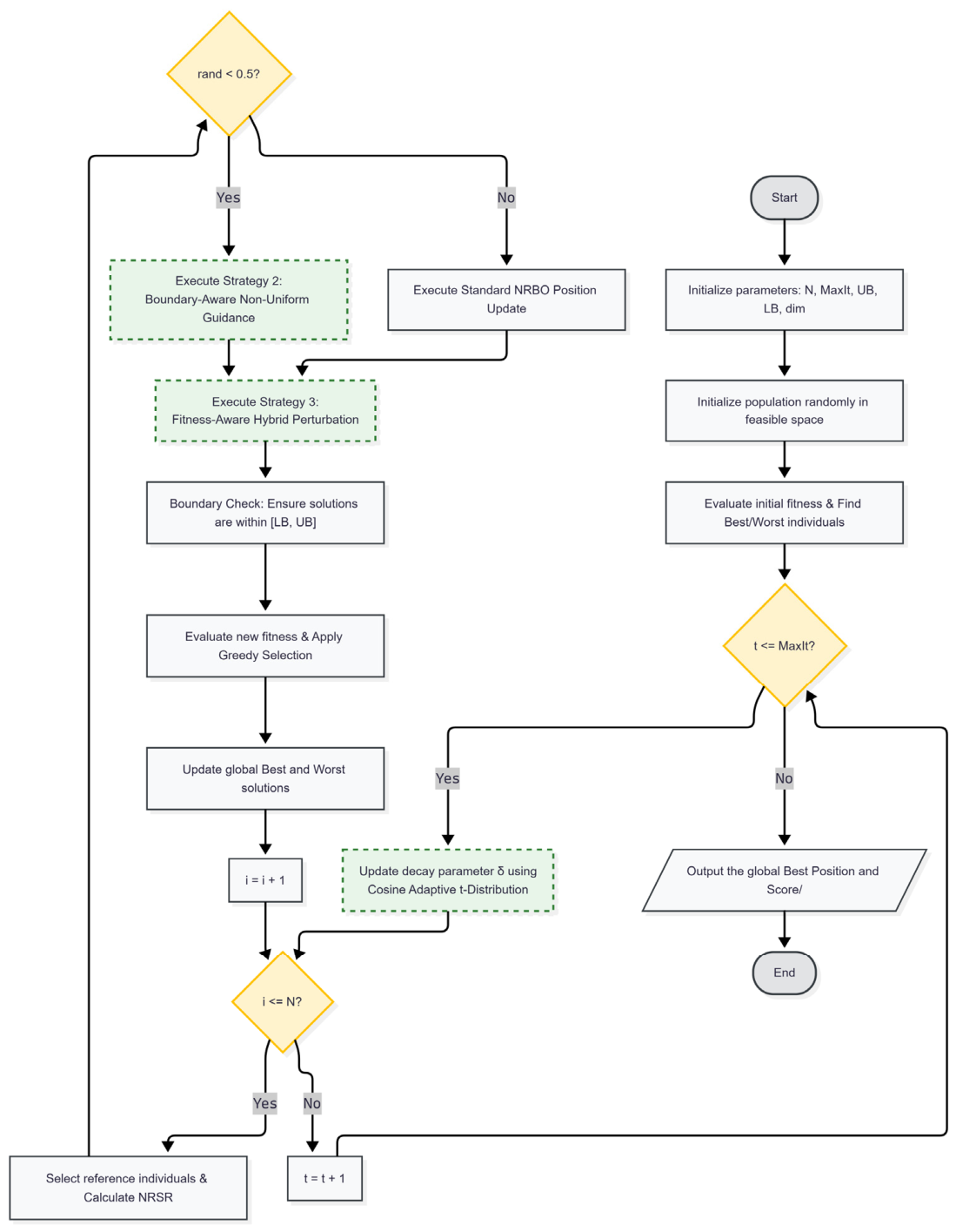
The general operating path of the proposed INRBO architecture is shown in Figure 1, and it can be seen from the three main sections that they are in good agreement: cosine-based adaptive t-distribution deviation, boundary-aware steering, and fitness-aware hybrid deviation.

2.4. The Proposed Double-Layer Optimized INRBO-SSA-LSTM Forecasting Architecture

2.4.1. SSA Parameter Optimization

In this paper, INRBO is used to optimize two key parameters in the SSA decomposition process: the window length M and the number of decomposition components K . For a given parameter combination M , K , SSA is first used to decompose the original load sequence into K components u i t , where i = 1 , 2 , , K . To evaluate the complexity of the SSA decomposition results under different parameter combinations, this paper adopts sample entropy as the fitness function. Sample entropy measures the complexity and irregularity of a time series; the smaller its value, the stronger the regularity of the series and the more stable the decomposition results.
Let the time series be u = u 1 , u 2 , , u N , the embedding dimension be m , and the similarity tolerance be r . Construct am -dimensional vector:
U m j = u j , u j + 1 , , u j + m 1 , j = 1 , 2 , , N m + 1
Calculate the maximum distance between any two vectors U m i and U m j , and compute the matching probability B m r that this distance is less than the tolerancer. Similarly, when the dimension is increased tom + 1 , the matching probability B m + 1 r is obtained. The sample entropy is defined as:
S a m p E n m , r , N = ln B m + 1 r B m r
In this paper, we set m = 2 and r = 0.2 σ , where σ is the standard deviation of the corresponding SSA component. For each SSA component u i t and, we calculate the sample entropy S E i , and take the minimum value among the sample entropies of all components as the fitness value for the current parameter combination:
f M , K = min i = 1 , 2 , , K S   E i
Therefore, the objective function for INRBO optimization of SSA parameters is expressed as:
M * , K * = arg min M , K f M , K
where M * and K * are the optimal window length and the optimal number of decomposition components obtained through optimization, respectively; m is the embedding dimension of the sample entropy; r is the similarity threshold; N is the sequence length; B m r and B m + 1 r represent the matching probabilities of the reconstruction vectors in the m -dimensional and m + 1 -dimensional spaces, respectively; and S E i represents the sample entropy of thei th SSA component. By minimizing sample entropy, INRBO is able to find SSA decompositions with lower complexity and greater regularity, thereby providing more stable and effective input features for subsequent LSTM prediction models.

2.4.2. The Proposed INRBO-SSA-LSTM Forecasting Framework

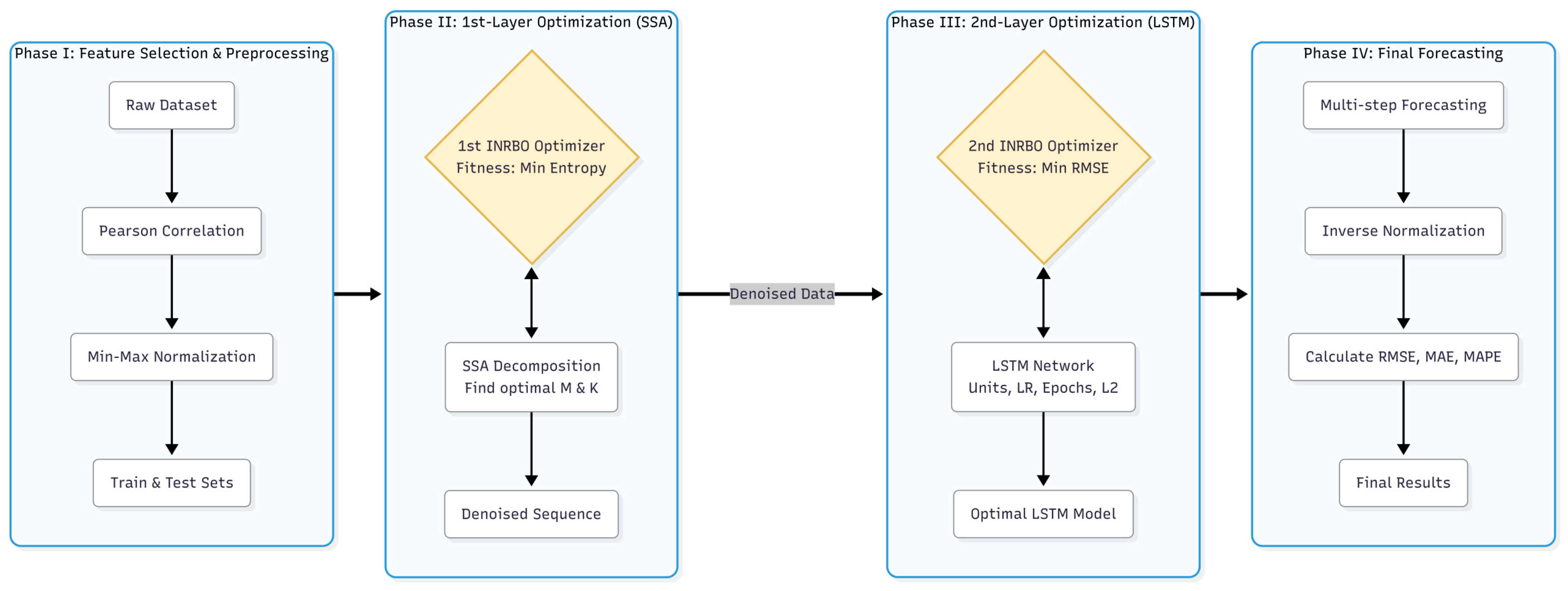
Although SSA and LSTM have a good theoretical foundation, they are not practical to use in terms of the tediousness and repetition of hyperparameter tuning. In order to build a general and strong prediction system, the following two-tier optimization plan was put forward: INRBO-SSA-LSTM. The overall four-stage execution pipeline of the proposed dual-layer automatic optimization architecture is visualized in Figure 2, and INRBO has made some progress in expanding its overseas distribution and will change the parameters of both the smoothing stage and the predictive architecture adaptively. In short, the whole process is as follows:
(1)
Phase I: Feature Selection and Data Preprocessing
Most of the first smart grid data repositories contain all kinds of weather information and data on the history of electricity consumption. To reduce the number of features and avoid too much noise in the training of a neural network, some essential indicators are first filtered by means of Pearson correlation. The strength of linear correlation between all weather variables and power consumption is expressed as the Pearson correlation coefficient, along with its corresponding p-value. Only the variables that are highly correlated and meet the statistical significance test will be included in the multi-dimensional input of the predictive model. Next, Min-Max Normalization will be applied to the cleaned data to speed up the learning process, and then sliding windows will be used to generate the necessary supervised training examples.
(2)
Phase II: First-Layer Optimization (Adaptive SSA Denoising)
First of all, INRBO can help to determine the optimal partition parameters for SSA; that is to say, the sliding window dimension ( M ) and the number of integrated principal components ( K ). Envelope Entropy (EE) or Sample Entropy (SE) of the reconstructed signal can be used as the objective function to measure the filtering performance of INRBO. Therefore, the scope of disorder is to be reduced and it will reach a relatively stable state with relatively small fluctuations. The polished signal is then passed on to the next stage.
(3)
Phase III: Second-Layer Optimization (Adaptive LSTM Forecasting)
Then, the altered load pattern is given to an LSTM. In the second stage, an extra autonomous INRBO will be employed to optimize some important hyperparameters of the LSTM structure, such as the number of hidden neurons, the starting learning rate, the maximum epoch limit and the L2 regularization term. The Root Mean Square Error (RMSE) of the training and validation datasets will be used as the evaluation index. Due to the high sensitivity of the boundary and the orientation of the fitness for INRBO, there is no local minimum in the LSTM configuration, so it has been chosen as an excellent model.
(4)
Phase IV: Final Forecasting and Evaluation
Set a reasonable set of hyperparameters, construct and train the whole LSTM model for multi-step demand forecasting on the test set. Next, the predicted results are inverted to obtain the initial magnitude, and all sorts of evaluation indices, such as RMSE, MAE, MAPE, etc., are used to assess how well the model works.
Decomposition of signals and advanced learning in a structured meta-heuristic optimization paradigm have been used to build a two-tier architecture that can carry out all-automatic hyperparameter tuning without manual operation or intuition bias.

3. Benchmark Testing of the Optimization Algorithm

In order to ensure the general robustness of the new INRBO, that is to say, it can perform well in all areas and avoid getting stuck in local optima, many tests must be conducted on benchmark data before it is applied to the problem of power consumption forecasting.

3.1. Analysis of the Effectiveness of Different Strategies

To further illustrate the specific contributions of the three improvement strategies to INRBO’s performance gains, this paper has conducted additional ablation experiments on the INRBO algorithm itself. Specifically, using the original NRBO as the baseline, we constructed algorithm variants NRBO1, NRBO2, and NRBO3, each incorporating a single improvement strategy, to analyze the impact of t-distribution perturbation, boundary-aware guidance, and fitness-aware hybrid perturbation on algorithm performance, respectively. Meanwhile, the complete INRBO—which integrates all three strategies—served as the final comparison object. The CEC2017 test functions were selected as the benchmark test set. This test set covers various types of complex optimization problems, including unimodal, multimodal, mixed, and composite functions, and can comprehensively evaluate the algorithm’s global search capability, local exploration capability, and ability to escape local optima. To minimize the impact of randomness on the experimental results, each algorithm was run multiple times independently on each test function under 10-dimensional conditions. The mean, standard deviation, and Friedman average rank were used as evaluation metrics to comprehensively reflect the optimization accuracy, stability, and overall ranking performance of the different algorithms.
As shown in the Table 1, in the 10-dimensional ablation experiments on the CEC2017 test set, the INRBO proposed in this paper achieved the best overall performance, with a Friedman mean of 1.724138, ranking first. This result is significantly better than that of the original NRBO and all individual improved variants, demonstrating that the fusion of multiple strategies can effectively enhance the algorithm’s comprehensive optimization performance. Compared with the original NRBO, INRBO achieved lower mean values on most test functions, with particularly pronounced advantages on functions such as F1, F12, and F30. This indicates that the improved strategies can significantly enhance the algorithm’s convergence capability and stability in complex search spaces.
Among the various ablation variants, NRBO2’s overall performance most closely resembles that of INRBO, while Friedman ranks second and achieves superior results on functions such as F5, F10, F13, F14, F15, F18, and F19, indicating that this strategy plays a positive role in enhancing local development capabilities and optimization accuracy for complex functions. NRBO3 ranked third, performing notably well on functions such as F1, F4, F12, and F26, indicating that it possesses good convergence accuracy for certain unimodal or specific complex functions; however, its overall stability remains weaker than that of INRBO. NRBO1 ranked fourth. Although it showed improvement over the original NRBO, its optimization performance on most functions was inferior to that of NRBO2 and NRBO3, indicating certain limitations in the improvement capabilities of a single strategy. The original NRBO ultimately ranked fifth, with relatively high mean and standard deviation values across multiple function types. The gap with INRBO was particularly evident in functions such as F1, F12, and F30, reflecting its shortcomings in global search, local exploration, and escaping local optima.
In summary, each individual improvement strategy was able to enhance NRBO’s performance on certain functions, validating the effectiveness of the different strategy designs; whereas INRBO, by integrating multiple improvement mechanisms, achieved a better balance between exploration capability, exploitation accuracy, and stability. Consequently, it attained the best overall ranking on the CEC2017 test set, demonstrating the effectiveness and necessity of the proposed multi-strategy collaborative improvement scheme.

3.2. CEC2017 Benchmark Tests with Different Dimensions

To further validate the applicability of INRBO in optimization problems with different dimensions, this paper conducted comparative experiments on the CEC2017 benchmark dataset for 10-dimensional, 30-dimensional, and 50-dimensional problems and compared INRBO with NRBO, SSOA, HHO, WOA, and AOA.
As shown by the experimental results listed in Table 2 (10 dimensions), Table 3 (30 dimensions) and Table 4 (50 dimensions), INRBO achieved the best overall ranking across all dimensions, demonstrating strong convergence accuracy, stability, and high-dimensional search capabilities. able 2 records the mean and standard deviation of all compared algorithms on the 10-dimensional CEC2017 benchmark functions. In the 10-dimensional test, INRBO achieved a Friedman mean ranking of 1.034483, placing first overall. It obtained optimal or near-optimal mean values on nearly all test functions, demonstrating favorable performance relative to other algorithms—particularly on complex functions such as F1, F12, F19, and F30—which indicates its high optimization accuracy and stability in low-dimensional problems.
As the dimension increased to 30, the computational difficulty for all algorithms rose significantly. The detailed statistical results under the 30-dimensional setting are summarized in Table 3. For some algorithms, the mean and standard deviation on complex functions experienced a moderate increase, while INRBO maintained its lead, with a Friedman mean ranking of 1.206897 and ultimately ranking first. In particular, for highly complex functions such as F1, F12, F13, F15, F18, F19, and F30, INRBO’s results were markedly superior to those of NRBO and other comparison algorithms, indicating that the proposed improvement strategy can effectively mitigate the expansion of the search space and the problem of local optima caused by increased dimensionality.
In the 50-dimensional experiments, the test problems became even more complex, yet INRBO still achieved the optimal result with a Friedman mean ranking of 1.137931, ultimately retaining the top position. Table 4 presents the full comparison data for the 50-dimensional CEC2017 test suite. Compared to NRBO, INRBO exhibited lower mean values and smaller fluctuations on most functions; Compared to HHO, WOA, AOA, and SSOA, INRBO’s advantages are even more pronounced on high-dimensional mixed and composite functions, demonstrating its superior global search and local exploration capabilities.
In summary, INRBO achieved the best overall ranking in the 10-dimensional, 30-dimensional, and 50-dimensional experiments on the CEC2017 test set, as verified by Table 2, Table 3 and Table 4 This proves that the algorithm is not only suitable for low-dimensional optimization problems but can also maintain good convergence performance and robustness in higher-dimensional search spaces, thereby validating the feasibility and effectiveness of the improved strategy.

3.3. Tests on the CEC2022 Benchmark Suite

To verify the optimization performance and robustness of the proposed INRBO algorithm on complex test functions, this paper adopts the CEC2022 benchmark function suite, which contains 12 test functions in total and falls into four categories: unimodal, multimodal, hybrid and composite. The average and standard deviation of the 30 trials are taken to assess the accuracy and consistency of the optimization. The detailed statistical results are shown in Table 5; that is to say, the maximum values of all objective functions are in bold.
As shown in Table 5, INRBO has the minimum Mean and Std for most of the evaluation scenarios. Therefore, it can be seen that the boundary-oriented guiding mechanism does not need to be explored extensively, and a good solution far from the source of the error can be obtained.
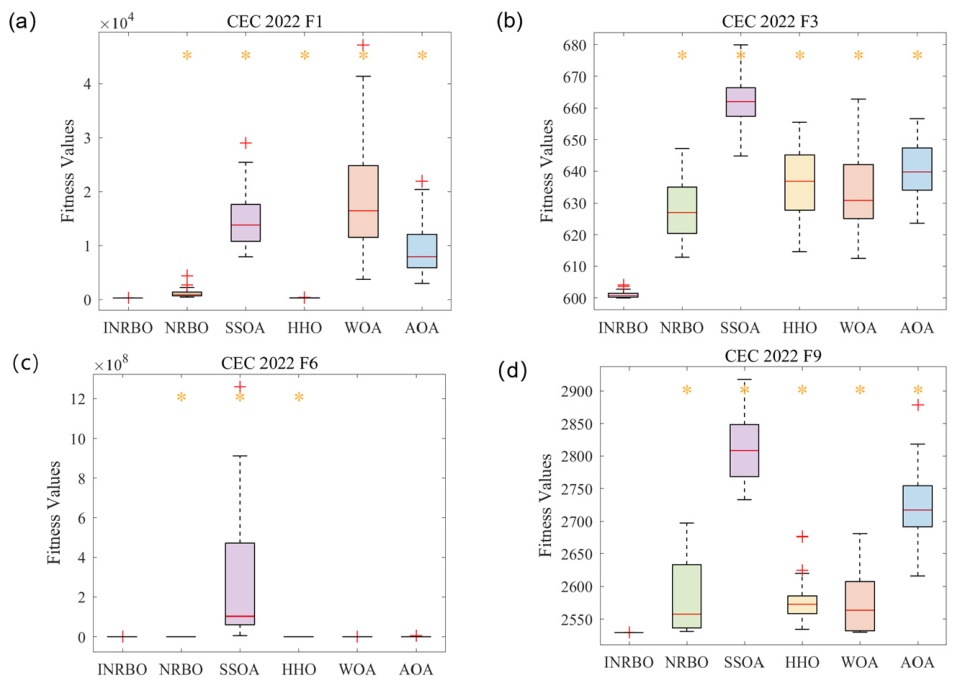
The speed of convergence and avoidance of local optima can be seen in the convergence path of a typical benchmark function. A box plot is used to show the spread of the 30 individual autonomous trials.
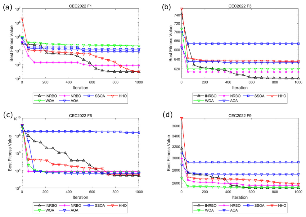
Figure 3 shows that the standard NRBO is often at a plateau initially in the diagrams. As the t-distribution has heavy tails, INRBO will show a “ladder” of diminishing in the last few iterations and will not get stuck in a regional optimum. In addition, the reduced spans of INRBO in Figure 4 are also very consistent.

3.4. Wilcoxon Rank-Sum and Friedman Tests

The mean and standard deviation are relatively normal, so although we will use a non-parametric test, we still need to know whether the increase in INRBO is statistically significant or just random fluctuations. The Wilcoxon rank-sum test will be used at the 5% significance level (p < 0.05). Finally, the overall mean rank of all the assessed algorithms in the 12 indicators can also be determined by the non-parametric Friedman test.
As shown in Table 6, almost all of the p-values for INRBO and other methods are less than 0.05, so we reject the null hypothesis, indicating that the performance differences are statistically significant. In addition, INRBO is at the top of the Friedman mean rank. Therefore, the above mathematical verification shows that INRBO is a good and stable optimizer; thus, it can be used as a strong foundation for the next step of deep learning model hyperparameter tuning.

4. Results and Discussion

4.1. Data Description and Feature Correlation Analysis

To know if the proposed INRBO-SSA-LSTM framework can be used in practice and to examine how accurate it is for forecasting, the actual electrical load data from an industrial area in Wuxi, Jiangsu Province, China, was collected. The information timeframe is the entire month of August, and there are 744 consecutive hourly observations. It is the history of active electricity consumption and the eight meteorological factors recorded at the same time.
When a large amount of climate data or a weak connection is added to the deep learning model in actual industrial electrical operation scenarios, it will result in a large number of computations and thus be prone to obvious overfitting and poor predictive generalization ability. To solve the problem of high dimensionality, Pearson Correlation Coefficients (PCC) are used to measure the strength of the linear relationship among all meteorological parameters and the electrical power target variable. For a particular sample population n , the PCC of the two variables x and y can be expressed as:
r = i = 1 n ( x i x ¯ ) ( y i y ¯ ) i = 1 n ( x i x ¯ ) 2 i = 1 n ( y i y ¯ ) 2
In light of this, x i and y i are specific observations, and x ¯ and y ¯ are the computed averages of the corresponding factors. The range of the correlation coefficient r is [ 1 , 1 ] . The value of r is relatively large, and at the same time, this same variable may be considered statistically significant based on its p-value.
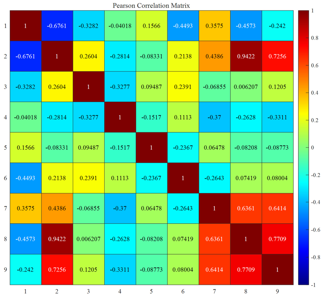
As shown in Figure 5, heatmap of Pearson Correlation Coefficients Among Climatic Variables and Actual Electrical Load is plotted. To address the problem of redundant meteorological features and reduce model computation volume, strict feature selection criteria have been set; that is to say, only variables with a relatively large absolute correlation coefficient ( | r | > 0.3 ) and a small p-value ( p < 0.01 )) will be selected.
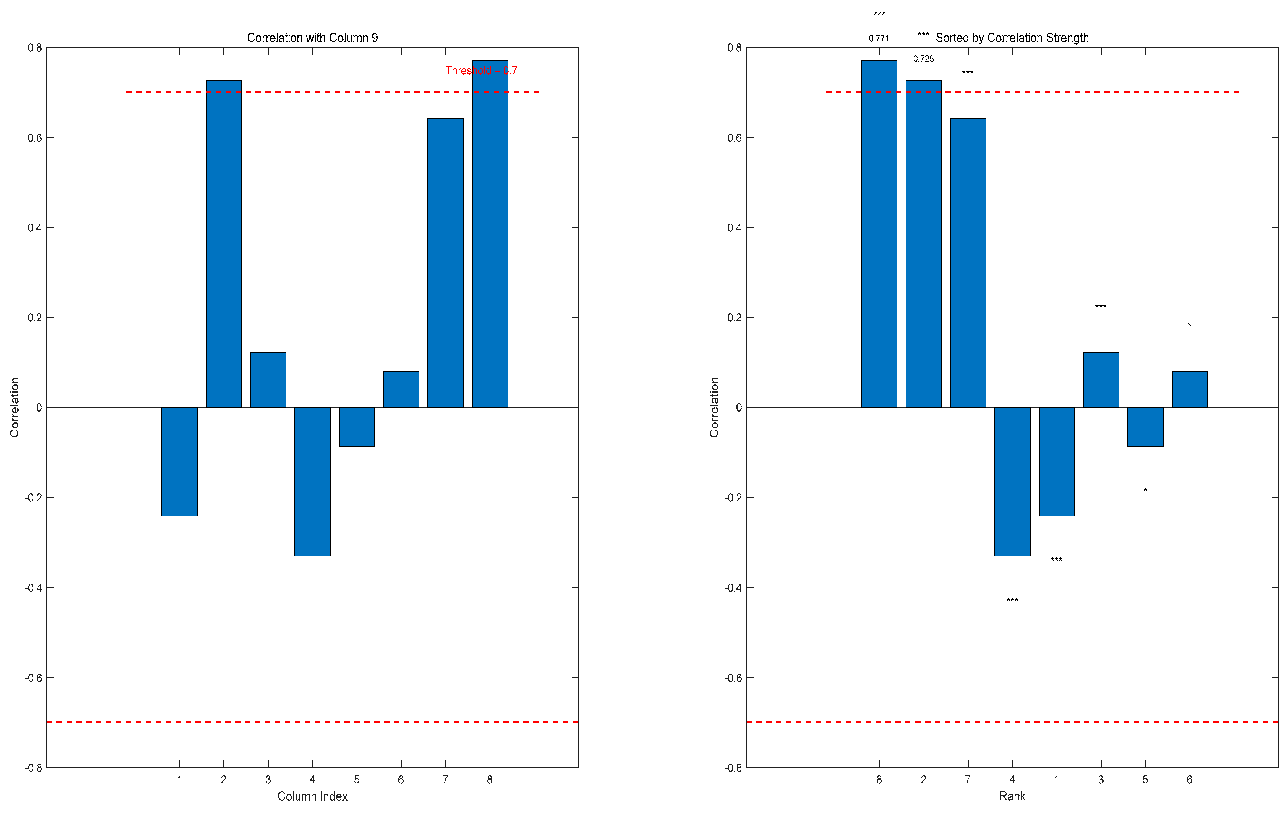
As shown in the correlation ranking analysis (Figure 6), only four meteorological factors were above the upper limit. The correlation coefficient of apparent temperature (Column 8) is 0.771; that of air temperature (Column 2) is 0.726; water vapor pressure (Column 7) is 0.641, and all of them positively correlate with energy consumption. Atmospheric Pressure (Column 4, r = −0.331) is still negatively correlated. The other variables do not meet the | r | > 0.3 criterion and are thus omitted. Therefore, according to the above strict mathematical screening method, the four necessary conditions have been determined and an optimized input dataset for the following deep learning forecasting framework has been prepared.

4.2. Evaluation Metrics

The four common indicators of the forecasting accuracy and stability of the proposed model are Root Mean Square Error (RMSE), Mean Absolute Error (MAE), Mean Absolute Percentage Error (MAPE) plus the coefficient of determination ( R 2 ). The relevant mathematical formulas are given in this paper.
R M S E = 1 n i = 1 n ( y i y ^ i ) 2
M A E = 1 n i = 1 n | y i y ^ i |
M A P E = 100 % n i = 1 n y i y ^ i y i
R 2 = 1 i = 1 n ( y i y ^ i ) 2 i = 1 n ( y i y ¯ ) 2
N is the total number of test cases in this formula, y i and y ^ i are the genuine and projected power consumption values at time i, and y is the average value of actual energy consumption. In other words, large errors in the forecast are considered outliers and will significantly increase the RMSE; at the same time, MAPE is proportional to the size of the error. A good prediction model should have small values for RMSE, MAE, MAPE and a high R-squared close to 1.

4.3. Signal Denoising and Hyperparameter Optimization Analysis

In short, the temporal order of basic power consumption is generally non-stationary and has a large degree of stochastic oscillation; thus, it is not suitable as a feature vector for LSTM directly. Singular Value Decomposition (SVD) is a relatively robust way to extract the basic trend from noisy data; however, there will still be residual noise, and it is not easy to choose an appropriate window length and the number of principal components. The empirical trial-and-error method is too subjective; thus, it cannot be analyzed properly.
To address the above issue, the first level of the proposed improved framework is to use the INRBO method to dynamically select an optimal [ M , K ] pair and reduce the entropy level of the isolated time series.
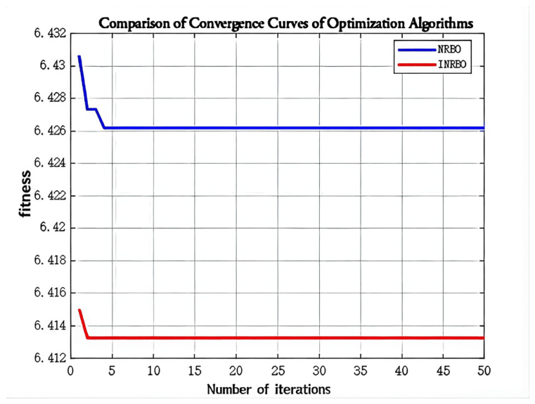
As shown in the convergence plots (Figure 7), the proposed INRBO has a faster convergence speed and can escape the local minima of NRBO; finally, it has reached a lower fitness value of 6.413245.
As shown in Table 7, the entire numerical evaluation is also in need of adjustment. The manual configuration of SSA (M = 30, K = 5) has the largest reconstruction deviation. On the other hand, INRBO has a larger window span (M = 36) and more components (K = 8). Based on the optimization above, the maximum signal-to-noise ratio is 15.87 dB and the corresponding root mean square error is about 9.2734. Based on the above reliable results, it can be seen that INRBO-optimized decomposition reduces random fluctuations and maintains the basic structure of electrical consumption; therefore, it has created a very stable dataset for the following predictive model.

4.4. Ablation Study and Forecasting Performance

4.4.1. Progressive Ablation Study of Prediction, Decomposition, and Optimization Modules

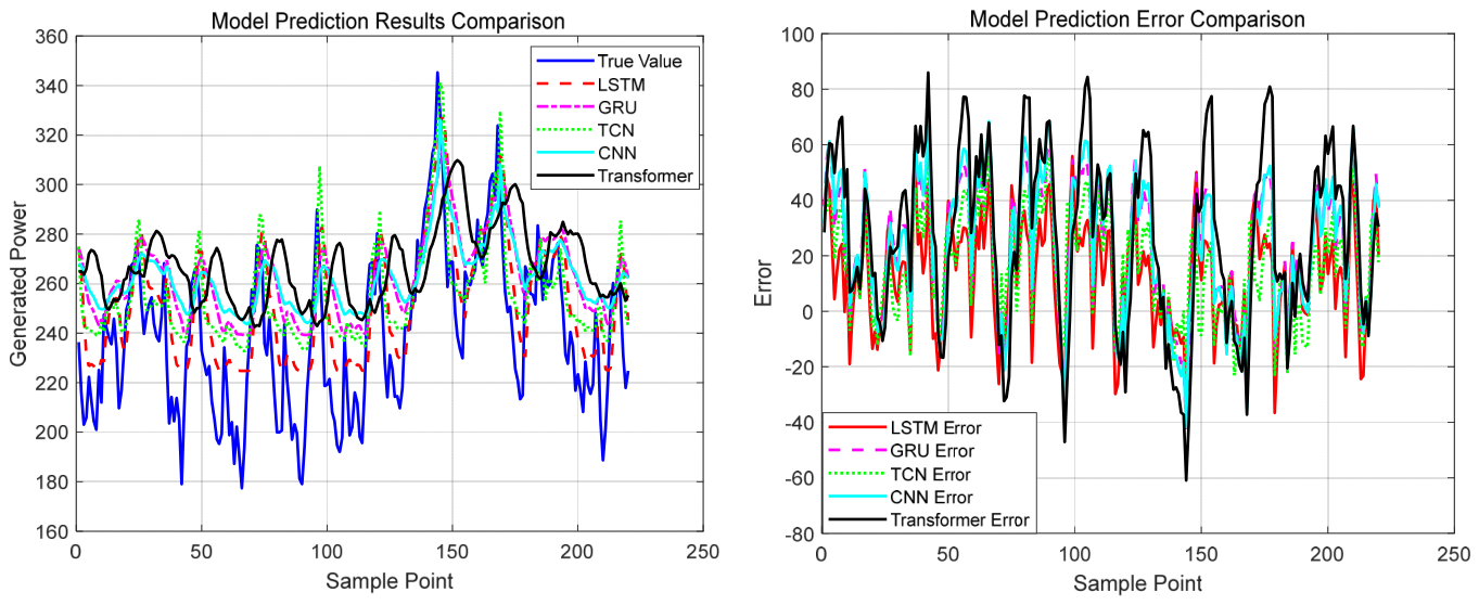
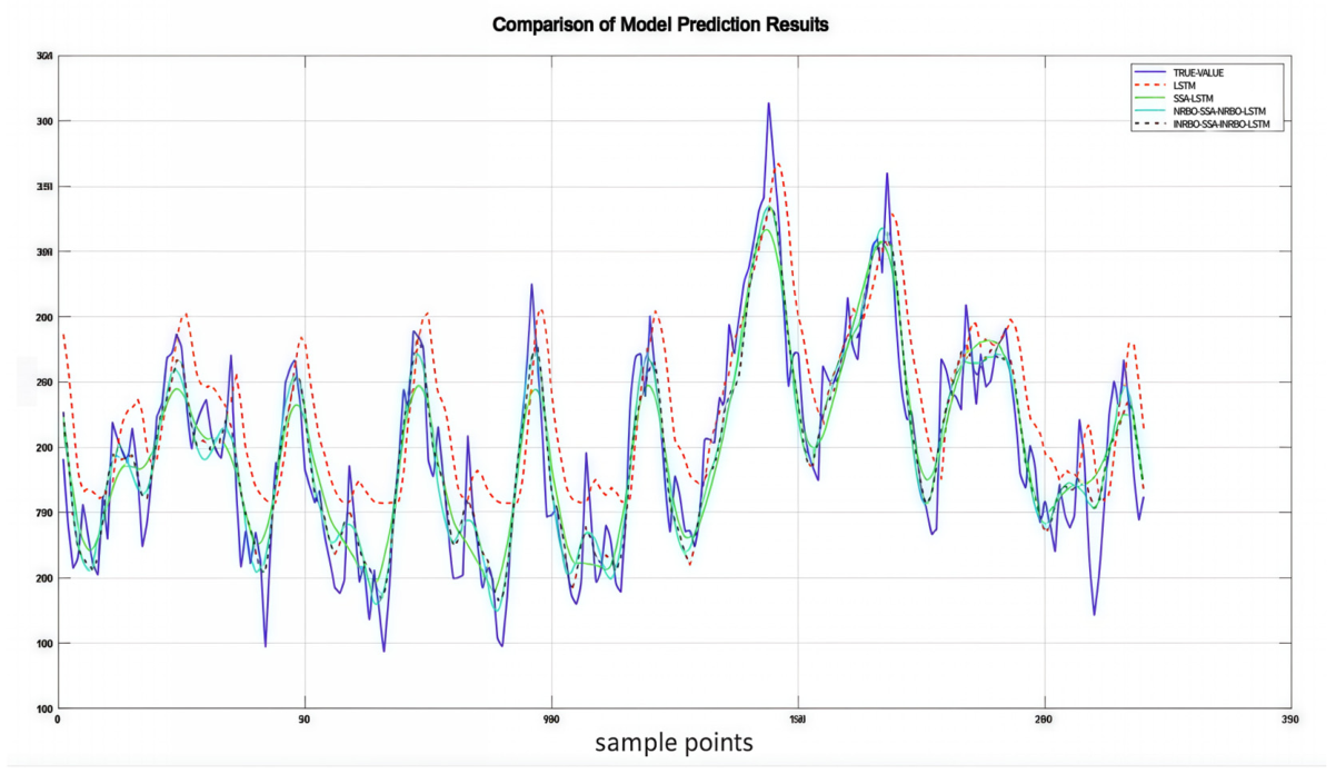
To more clearly reveal the roles of each component module in the proposed model, this paper redesigned the ablation experiments following a progressive approach: from basic prediction models to decomposition-based combination models and finally to algorithm parameter optimization models. First, we conducted comparative experiments on basic prediction models such as LSTM, GRU, TCN, CNN, and Transformer to determine the basic prediction architecture to be adopted in subsequent combination models. Second, after the base prediction model was determined, we further compared the prediction performance of decomposition methods—such as SSA, EMD, VMD, and CEEMDAN—when combined with LSTM to analyze the impact of the decomposition preprocessing module on model performance. Finally, based on the established decomposition-combination model, we compared the effects of different optimization algorithms on LSTM parameter tuning to verify the contribution of the INRBO optimization module to the final prediction performance. The specific prediction results and error curves for the selected benchmark models are shown in Figure 8.
As shown in the benchmark model comparison figure, each individual prediction model is able to track load trend changes to a certain extent; however, deviations of varying degrees still exist during local peaks, troughs, and periods of rapid fluctuation. Among them, the LSTM captures time-dependent relationships relatively well, with its prediction curve exhibiting better alignment with the actual curve than the other benchmark models; GRU, CNN, and TCN exhibit lag or amplitude deviations in certain inflection points, while the Transformer shows more pronounced fluctuation errors given the current sample size. Thus, without introducing decomposition or optimization strategies, the LSTM has already demonstrated relatively stronger time-series modeling capabilities. For further validation, detailed evaluation metrics are presented in Table 8.
As shown in the benchmark model comparison table, LSTM performed best among the individual models, with MAE, RMSE, and MAPE of 19.4959, 23.1557, and 8.63%, respectively; TCN ranks second, while the Transformer has the highest error. These results indicate that LSTM is more suitable for handling the load forecasting task in this paper than other baseline models; however, its error level remains relatively high, suggesting that relying solely on a single forecasting model is insufficient to fully capture the non-stationary fluctuations in the original time series. Therefore, after establishing LSTM as the baseline forecasting model, we further introduced different decomposition methods to construct decomposition-combination models. The specific results are shown in Figure 9.
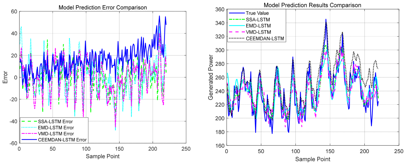
After establishing LSTM as the baseline prediction model in the first set of experiments, the second set of experiments further compared the prediction performance of LSTM combined with different decomposition methods. As shown in the comparison chart of decomposition-combined models, the introduction of signal decomposition caused the prediction curves of all combined models to generally align more closely with the actual values. This indicates that decomposition preprocessing reduces the complexity of the original load sequence, making it easier for LSTM to learn the patterns of variation in different frequency components. Compared to EMD, VMD, and CEEMDAN, SSA-LSTM exhibits smaller deviations at peak and valley positions as well as at inflection points in fluctuations, indicating that the components obtained after SSA decomposition exhibit better regularity and predictability. Specific evaluation metrics are shown in Table 9.
As shown in the comparison table of decomposition-combination models, SSA-LSTM achieved the best results, with MAE, RMSE, and MAPE of 11.1109, 13.6583, and 4.76%, respectively. Compared with the single LSTM, the SSA-LSTM reduced MAE and RMSE by approximately 43.01% and 41.02%, respectively, and lowered MAPE by 3.87 percentage points, indicating that the SSA decomposition module can significantly improve the quality of input features. Based on these results, subsequent experiments further incorporated algorithm parameter optimization into the SSA decomposition and LSTM prediction framework to verify the performance gains achieved by the optimization algorithm. The specific results are shown in Figure 10.
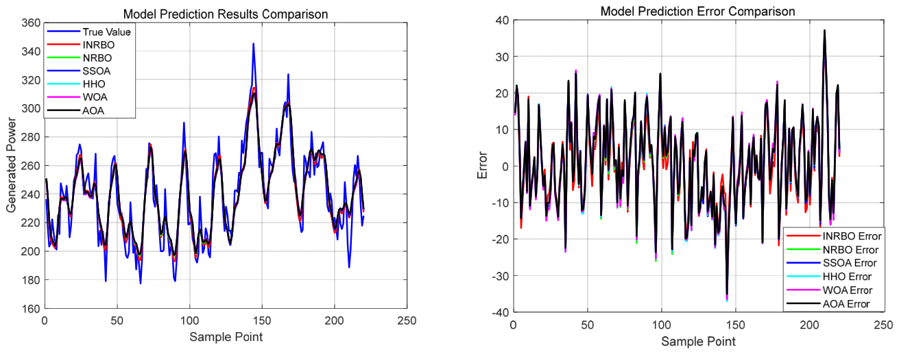
After establishing the baseline LSTM prediction model and the SSA decomposition method in the first two sets of experiments, the third set of experiments further compared the effects of different optimization algorithms on LSTM parameter optimization. As shown in the comparison of models using different optimization algorithms, under the condition of a fixed INRBO-SSA decomposition input, different optimization algorithms primarily affect the quality of LSTM parameter combinations and the degree of local fit of the prediction curves. The prediction curve of the INRBO-SSA-LSTM model is overall closest to the true values, with relatively smaller deviations at peaks, troughs, and in continuous fluctuation intervals. This indicates that INRBO achieves superior global optimization results when searching for key LSTM parameters. Specific evaluation metrics are shown in Table 10.
As shown in the comparison table of optimization models based on different algorithms, the MAE, RMSE, and MAPE of the INRBO-SSA-LSTM model are 8.7393, 10.8314, and 3.72%, respectively, all of which outperform the NRBO, SSOA, HHO, WOA, and AOA optimization models. Compared with SSA-LSTM, this model further reduces MAE and RMSE by approximately 21.34% and 20.70%, respectively, and lowers MAPE by 1.04 percentage points; compared with INRBO-SSA-NRBO-LSTM, MAE and RMSE are reduced by approximately 8.25% and 8.19%, respectively. In summary, the three sets of experiments above demonstrate a clear progressive improvement in model performance: first, LSTM exhibits strong time-series modeling capabilities in the baseline prediction model; second, SSA decomposition effectively reduces the complexity of the original sequence, enhancing the quality of LSTM input features; and finally, INRBO further optimizes key LSTM parameters, leading to a continued reduction in prediction error. These results indicate that the performance improvement of the proposed model stems from the synergistic effects of the three components—baseline prediction, decomposition preprocessing, and parameter optimization—and validate that the proposed INRBO-SSA-LSTM model can effectively improve prediction accuracy.

4.4.2. Comparative Experiments Across Different Months

To address the issue of insufficient seasonal diversity, this paper further selected load data from January, May, and December to conduct cross-month comparison experiments. The three test months correspond to different meteorological conditions and fluctuations in industrial electricity consumption and can, to a certain extent, reflect the model’s generalization ability under load variation scenarios in winter, the spring-summer transition period, and year-end. Since the effectiveness of each module was already validated in the previous section, this experiment does not include ablation studies. Instead, all comparison models use the same data partitioning method, input variables, SSA decomposition strategy, and LSTM training conditions; only the LSTM parameter optimization algorithm is varied to ensure consistency in the comparison between different algorithms. The evaluation metrics remain MAE, RMSE, and MAPE, where lower values indicate lower prediction errors.
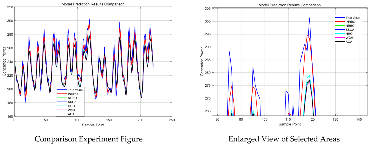
As shown in Figure 11, in the January load sequence, all optimized models were able to track the overall trend, but deviations of varying degrees still existed in local peaks, troughs, and periods of rapid fluctuations. Compared with the NRBO, SSOA, HHO, WOA, and AOA optimization models, the prediction curve of the INRBO-SSA-LSTM model aligns more closely with the actual load curve, and the local magnified views show smaller deviations in peak and trough positions, indicating that the proposed model possesses better dynamic tracking capabilities under winter load fluctuation scenarios. To further quantify the prediction errors of different models, the evaluation metrics for January are shown in Table 11.
As shown in Table 11, the INRBO-SSA-LSTM model achieved the best prediction results in the January experiment, with MAE, RMSE, and MAPE of 5.9071, 7.5398, and 2.47%, respectively. Compared with the other model that performed best in the same month—INRBO-SSA-HHO-LSTM—the proposed model reduced MAE and RMSE by approximately 36.03% and 35.91%, respectively, and lowered MAPE by 1.31 percentage points. These results indicate that, under the conditions of significant peak-to-valley load variations in January, INRBO’s optimization of key LSTM parameters can further reduce prediction errors. The comparison chart for May is shown in Figure 12.
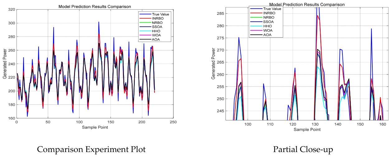
As shown in Figure 12, the fluctuation pattern of the load curve in May differs from that in January; load changes are smoother, but local inflection points remain relatively pronounced. All comparison models demonstrate a certain degree of predictive capability regarding the overall trend, but amplitude deviations still occur near continuous fluctuations and local extrema. The prediction curve of the INRBO-SSA-LSTM model is closer to the actual values at most time points, and the lag phenomenon and amplitude errors in the locally magnified regions are relatively smaller, indicating that this model can maintain good predictive stability during the transition months between spring and summer. The evaluation metrics for each model in May are shown in Table 12.
As shown in Table 12, in the May experiments, the MAE, RMSE, and MAPE of the INRBO-SSA-LSTM model were 5.5114, 7.3276, and 2.48%, respectively, all of which were the best values among all models. Compared with INRBO-SSA-AOA-LSTM—the other model with the lowest error in that month—the proposed model reduced MAE and RMSE by approximately 32.49% and 28.90%, respectively, and lowered MAPE by 1.19 percentage points. These results indicate that under varying meteorological and load conditions in May, the proposed two-layer optimized forecasting framework still maintains low error and demonstrates good cross-month adaptability. The comparison chart for December is shown in Figure 13.
As shown in Figure 13, the load curve for December also exhibits certain peak-to-trough variations and local fluctuations. Compared with other optimization models, INRBO-SSA-LSTM demonstrates higher fitting accuracy in terms of overall trends, local peaks, and trough intervals; the local zoom-in view shows minimal deviation between the predicted curve and the actual curve. This phenomenon indicates that, under the year-end winter load scenario, the proposed model is still capable of effectively capturing the primary patterns of change in the load sequence. The evaluation metrics for each model in December are shown in Table 13.
As shown in Table 13, in the December experiments, the MAE, RMSE, and MAPE of INRBO-SSA-LSTM were 5.6948, 7.4021, and 2.18%, respectively, which still outperformed other optimized models. Compared with INRBO-SSA-AOA-LSTM—the other model with the lowest error in that month—the proposed model reduced MAE and RMSE by approximately 15.75% and 14.83%, respectively, and lowered MAPE by 0.40 percentage points. Although the error gap between models in December narrowed relative to January and May, INRBO-SSA-LSTM still maintained the best results, indicating that its predictive advantage does not rely solely on the data distribution of a specific month.
A comprehensive analysis of the three sets of cross-month experiments—for January, May, and December—shows that INRBO-SSA-LSTM achieved the lowest MAE, RMSE, and MAPE across all months, with MAPE values of 2.47%, 2.48%, and 2.18%, respectively, demonstrating relatively stable prediction accuracy. Compared with other optimized models, the proposed model can track the actual load curve more accurately under various load fluctuation conditions and exhibits smaller deviations during local peaks and troughs as well as in rapidly changing intervals. The above results further demonstrate that the two-layer optimized forecasting framework proposed in this paper not only achieves high forecasting accuracy in the original experimental months but also maintains good generalization ability and robustness on the supplementary cross-month data, thereby enhancing the reliability of the conclusions in this paper.

4.5. Discussion on the Robustness and Extremum Capturing Ability of Models

In addition to having good overall forecasting accuracy, it should also be flexible and stable when the load changes drastically, for example, at peak hours or during changes in the environment and industrial production, so as to ensure the normal operation of the plant microgrid. The system had good results in the base period, but they dropped in the peak period and resulted in severe power imbalances and infrastructure failures.
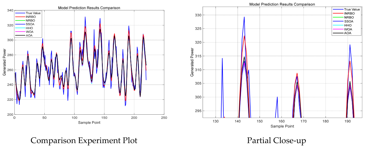
As shown in Figure 14, the prediction accuracy at the critical inflection point is presented; the traditional baseline structure (which includes classical LSTM and empirical SSA-LSTM) has a relatively long forecasting lag, that is to say, the projected trajectory is shifted to the right, and there is a considerable underprediction in the peak period. Even the single-layer improved NRBO-SSA-NRBO-LSTM cannot solve the problem of high-frequency oscillation in time. On the other hand, as shown in the close-up curve, the projected trajectory of the proposed INRBO-SSA-LSTM framework is very close to the actual active power load pattern, it can smoothly identify sharp peaks and troughs, and does not have a large delay.
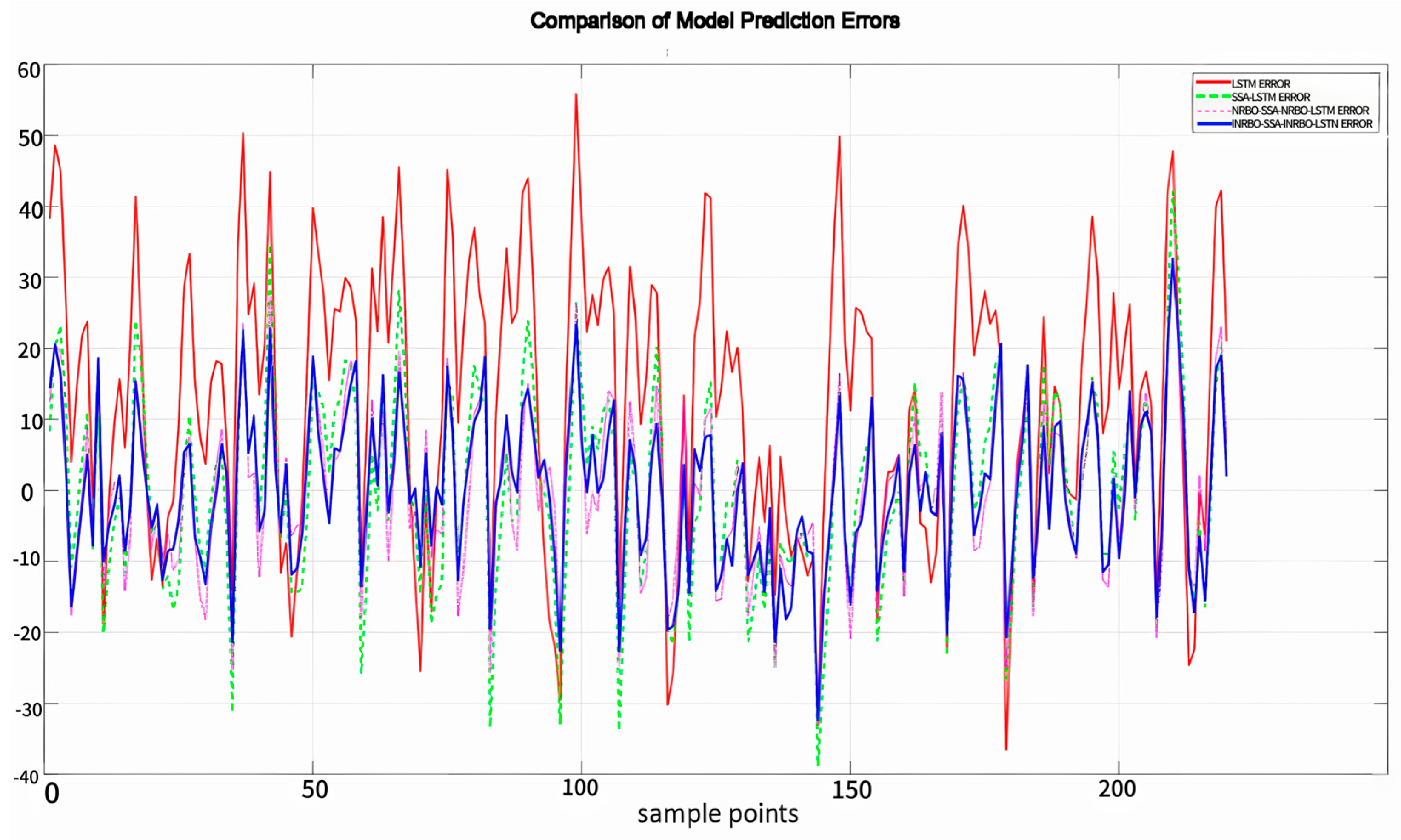
The good outlook is also supported by the quantitative data shown in the dynamic deviation surveillance illustration of Figure 15. The entire error trajectory of the baseline method is very fluctuating, and it has a prominent-frequency peak in the high-peak interval; at the same time, the absolute error of the proposed framework is still very condensed and consistently dispersed tightly around the zero axis. Under extreme conditions, there is a certain uniformity that can help the proposed architecture prevent electrical unbalance effectively, strengthen power reserve scheduling, and maintain the stability of the electrical grid; thus, it has shown some practical value in the field of modern intelligent industrial power management.

5. Conclusions

5.1. Conclusion

To maintain the normal operation of the power grid today, we need accurate short-term load forecasts. Given the problems of hyperparameter tuning and different energy consumption in deep learning, this paper proposes the theory of an improved Newton-Raphson-Based Optimizer (INRBO) to solve these problems and then develops a new dual-level optimization prediction framework (INRBO-SSA-LSTM). Based on the above assessment of traditional mathematical norms and empirical data collection from the microgrid, the main results are as follows:
(1)
Good algorithmic performance: According to all kinds of evaluations in the CEC2022 benchmark suite, it can be seen that the proposed INRBO is better than the traditional NRBO and many advanced swarm-based methods (such as WOA, HHO) in terms of search accuracy, convergence speed and stability. Based on the results of the Wilcoxon rank-sum test and Friedman mean ranking, both are p < 0.05 , and thus the combined multi-strategy architecture can solve the problem of local optima in high-dimensional spaces.
(2)
Practicability of Dimension Reduction: In order to reduce the number of features in the actual meteorological-load data, Pearson correlation coefficient (PCC) evaluation has been used to reduce the eight features to four essential climate factors (Temperature, Pressure, Water Vapor Pressure and Apparent Temperature). Pre-processing is done to reduce the curse of dimensionality and over-fitting of the model.
(3)
Accurate Adaptive Signal Filtering: Use the good optimization ability of INRBO to solve the problem of manual setting of parameters in Singular Spectrum Analysis (SSA). Determined a reasonable size for the window and the number of principal components ( M = 36 , K = 8 ) dynamically in INRBO-SSA to achieve a relatively high signal-to-noise ratio of 15.87 dB and filter out high-frequency random fluctuations in the basic load pattern effectively.
(4)
Good predictive accuracy and flexibility of stability: All the time in the prediction period, the two-tier structure has been able to find globally optimal hyperparameters for the LSTM model. Ablation analysis shows that our method is better than all the benchmark alternatives in all aspects, with a very small prediction error (MAE = 8.8992, RMSE = 10.9764, MAPE = 3.7866%) and a good R 2 value of 0.9741. It should be pointed out that in the event of a sudden peak-and-trough load fluctuation, the system has good dynamic stability and peak-capture ability, so it is a very reliable reference for microgrid power scheduling.

5.2. Limitations and Future Work

Although some are reasonably accurate, they are not perfect. Only in a certain industrial manufacturing microgrid area and based on short-term weather data has the current model been validated; it has not been applicable for an extended period of time due to changes in the global economy and problems of regional power grids. The calculation cost of the bi-level optimization method is too high because it needs to be updated frequently in the peripheral area of hardware-constrained devices.
The next investigation will focus on the two above paths. First, expand the scope of application for INRBO-SSA-LSTM to all parts of the country and investigate all reasons that affect electricity prices in large distribution systems. In order to improve the accuracy of the architecture in the edge computing environment and extend the functions of smart grid systems, a reasonable model compression method will be used.
It should be noted that this paper uses the Pearson correlation coefficient for feature selection, with the primary objective of performing preliminary dimensionality reduction on meteorological variables prior to modeling. This reduces the interference caused by weakly correlated and redundant variables during model training, thereby lowering computational complexity and the risk of overfitting. The Pearson correlation coefficient offers advantages such as simplicity of calculation, intuitive results, and strong interpretability, making it suitable as a preliminary screening method for input variables in load forecasting models. However, the Pearson correlation coefficient primarily reflects linear relationships between variables and struggles to fully capture the potential nonlinear relationships and time lag effects that may exist between meteorological factors and electricity load. Therefore, in subsequent research, we will further integrate methods such as mutual information, maximum information coefficient, distance correlation coefficient, cross-correlation analysis, Granger causality test, and feature importance analysis based on SHAP scores to conduct a more comprehensive exploration of the complex relationships between meteorological variables and electricity load, thereby further enhancing the rationality of feature selection and the generalization capability of the prediction model.

Author Contributions

Conceptualization, J.L. and F.C.; methodology, J.L. and F.C.; software, F.C.; validation, F.C., L.K. formal analysis, F.C. investigation, F.C. and L.K.; resources, J.L. and H.L.; data curation, L.K. writing—original draft preparation, F.C.; writing—review and editing, J.L., H.L. and F.C.; visualization, F.C.; supervision, J.L. and H.L.; project administration, J.L.; funding acquisition, J.L. All authors have read and agreed to the published version of the manuscript.

Funding

This research was funded by the Project of the Educational Department of Liaoning Province, grant number LJ242511632005.

Institutional Review Board Statement

Not applicable.

Informed Consent Statement

Not applicable.

Data Availability Statement

The data presented in this study are available on request from the corresponding author. The data are not publicly available due to privacy restrictions regarding the commercial electricity consumption of the industrial microgrid.

Conflicts of Interest

The authors declare no conflicts of interest.

References

  1. Zhu, G.; Zhang, S.; Deng, Z.; Wang, J.; Li, Y.; Dong, J.; Bauer, P. Extended hybrid modulation for multistage constant-current wireless EV charging. IEEE Trans. Power Electron. 2025, 40, 10095–10110. [Google Scholar] [CrossRef]
  2. Liu, B.; Wu, J.; Chai, L. Distributed Privacy-Preserving Algorithm for Economic Dispatch and Demand Response of Smart Grid with Homomorphic Encryption. IEEE Trans. Smart Grid 2025, 16, 173–182. [Google Scholar] [CrossRef]
  3. Akhtar, S.; Shahzad, S.; Zaheer, A.; Ullah, H.S.; Kılıç, H.; Goňo, R.; Jasinski, M.L.; Leonowicz, Z. Short-Term Load Forecasting Models: A Review of Challenges, Progress, and the Road Ahead. Energies 2023, 16, 4060. [Google Scholar] [CrossRef]
  4. Anusha, T.G.; Vinod, A.; Binas, M.S.; Kumar, S.; Bindu, C.J. A Comprehensive Review of the Short-Term Load Forecasting Techniques Using Different Models. In Proceedings of the 2025 2nd International Conference on Trends in Engineering Systems and Technologies (ICTEST), Kochi, India, 3–5 April 2025; pp. 1–6. [Google Scholar]
  5. Jafari, M.; Kavousi-fard, A.; Chen, T.; Karimi, M. A Review on Digital Twin Technology in Smart Grid, Transportation System and Smart City: Challenges and Future. IEEE Access 2023, 11, 17471–17484. [Google Scholar] [CrossRef]
  6. Iyaniwura, A.A.; Mayaki, C.S. Artificial Intelligence-enabled smart grid systems for real-time load forecasting, fault detection, renewable energy integration and optimization. Glob. J. Eng. Technol. Adv. 2025, 10, 191–208. [Google Scholar] [CrossRef]
  7. Dabe, N.P.; Kukarni, K.S.; Kadlag, S.S.; Dandotia, A.; Gupta, M.K.; Tiwari, A. Hybrid Generative AI for Smart Grid Load Forecasting with Renewable Energy Integration. In Proceedings of the 2025 World Conference on Cutting-Edge Science and Technology (WCCEST), Indore, India, 24–26 September 2025; pp. 1–6. [Google Scholar]
  8. Ahmed, M.M.; Mirsaeidi, S.; Koondhar, M.A.; Karami, N.; Tag-Eldin, E.M.; Ghamry, N.A.; El-Sehiemy, R.A.; Alaas, Z.M.; Mahariq, I.; Sharaf, A.M. Mitigating Uncertainty Problems of Renewable Energy Resources Through Efficient Integration of Hybrid Solar PV/Wind Systems into Power Networks. IEEE Access 2024, 12, 30311–30328. [Google Scholar] [CrossRef]
  9. Patel, V.R.; Makwana, V.H. Short-Term Solar and Wind Power Forecasting Using Machine Learning Algorithms for Microgrid Operation. Energies 2025, 19, 550. [Google Scholar]
  10. Liu, Y.; Zheng, R.; Liu, M.; Zhu, J.; Zhao, X.; Zhang, M. Short-Term Load Forecasting Model Based on Time Series Clustering and Transformer in Smart Grid. Electronics 2025, 14, 230. [Google Scholar] [CrossRef]
  11. Karima, N.N.; Syafruddin, W.A.; Mahfud, M.; Subiyanto, L.; Setiadi, H. Enhancing Short-Term Load Forecasting Using Hyperparameter-Optimized Deep Learning Approaches. Energies 2025, 19, 705. [Google Scholar] [CrossRef]
  12. Asiri, M.M.; Aldehim, G.; Alotaibi, F.A.; Alnfiai, M.M.; Assiri, M.; Mahmud, A. Short-Term Load Forecasting in Smart Grids Using Hybrid Deep Learning. IEEE Access 2024, 12, 23504–23513. [Google Scholar] [CrossRef]
  13. Ertürk, M.; Emeç, M.; Turhan, M. Hybrid Deep Learning and Transformer-Based Framework for Multivariate Electricity Consumption Forecasting. Appl. Sci. 2026, 16, 2760. [Google Scholar] [CrossRef]
  14. Sakib, M.; Mustajab, S. CEEMDAN-TCN-AutoLSTM: A Triple-Force Ensemble Using Cross-Stitch Networks for Short-Term Load Forecasting. Arab. J. Sci. Eng. 2025, 50, 19939–19970. [Google Scholar] [CrossRef]
  15. Zhang, A.; Zhang, S.; Li, G. Research on CNN-LSTM Power Load Forecasting Model Based on Attention Mechanism. In Proceedings of the 2025 International Conference of Clean Energy and Electrical Engineering (ICCEEE), Changchun, China, 18–21 July 2025; pp. 1–5. [Google Scholar]
  16. Pentsos, V.; Tragoudas, S.; Wibbenmeyer, J.; Khdeer, N. A Hybrid LSTM-Transformer Model for Power Load Forecasting. IEEE Trans. Smart Grid 2025, 16, 2624–2634. [Google Scholar] [CrossRef]
  17. Kong, W.; Dong, Z.Y.; Jia, Y.; Hill, D.J.; Xu, Y.; Zhang, Y. Short-Term Residential Load Forecasting Based on LSTM Recurrent Neural Network. IEEE Trans. Smart Grid 2019, 10, 841–851. [Google Scholar] [CrossRef]
  18. Rafi, S.H.; Nahid-Al-Masood, N.A. Highly Efficient Short Term Load Forecasting Scheme Using Long Short Term Memory Network. In Proceedings of the 2020 8th International Electrical Engineering Congress (iEECON), Chiang Mai, Thailand, 4–6 March 2020; pp. 1–4. [Google Scholar]
  19. Yin, S.; Chen, Z.; Liu, W.; Su, Z. Ultra Short-Term Charging Load Forecasting Based on Improved Data Decomposition and Hybrid Neural Network. IEEE Access 2025, 13, 58778–58789. [Google Scholar] [CrossRef]
  20. Aswanuwath, L.; Pannakkong, W.; Buddhakulsomsiri, J.; Karnjana, J.; Huynh, V. A Hybrid Model of VMD-EMD-FFT, Similar Days Selection Method, Stepwise Regression, and Artificial Neural Network for Daily Electricity Peak Load Forecasting. Energies 2023, 16, 1860. [Google Scholar] [CrossRef]
  21. Pham, M.; Nguyen, M.; Wu, Y. A Novel Short-Term Load Forecasting Method by Combining the Deep Learning with Singular Spectrum Analysis. IEEE Access 2021, 9, 73736–73746. [Google Scholar] [CrossRef]
  22. Stratigakos, A.C.; Bachoumis, A.; Vita, V.; Zafiropoulos, E.P. Short-Term Net Load Forecasting with Singular Spectrum Analysis and LSTM Neural Networks. Energies 2021, 14, 4107. [Google Scholar] [CrossRef]
  23. Neeraj, N.; Mathew, J.; Behera, R.K. Power load forecasting based on long short term memory-singular spectrum analysis. Energy Syst. 2021, 13, 789–811. [Google Scholar] [CrossRef]
  24. Kaur, S.; Bala, A.; Parashar, A. A hybrid PSO-LSTM-based electricity prediction and optimization technique for home appliances. Sci. Technol. Energy Transit. 2026, 81, 132. [Google Scholar] [CrossRef]
  25. Hou, B.; Zhou, Y.; Liu, R.; Zhang, H. PSO-LSTM-Based Ultra-Short-Term Load Forecasting Study for Solar Heating System. Energies 2025, 18, 6254. [Google Scholar] [CrossRef]
  26. Ning, Y.; Wang, J.; Wang, Z.; Zhu, Y.; Zhang, J. Electricity Load Forecasting Method Based on Improved PSO-LSTM Modeling. In Proceedings of the 2025 International Conference on Power Electronics and Electric Drives (PEED), Dali, China, 7–9 March 2025; pp. 56–60. [Google Scholar]
  27. Mirjalili, S.; Lewis, A. The whale optimization algorithm. Adv. Eng. Softw. 2016, 95, 51–67. [Google Scholar] [CrossRef]
  28. Tian, D.; Shi, Z. MPSO: Modified particle swarm optimization and its applications. Swarm Evol. Comput. 2018, 41, 49–68. [Google Scholar] [CrossRef]
  29. Bozorgi, S.M.; Yazdani, S. IWOA: An improved whale optimization algorithm for optimization problems. J. Comput. Des. Eng. 2019, 6, 243–259. [Google Scholar] [CrossRef]
  30. Heidari, A.A.; Mirjalili, S.; Faris, H.; Aljarah, I.; Mafarja, M.; Chen, H. Harris hawks optimization: Algorithm and applications. Future Gener. Comput. Syst. 2019, 97, 849–872. [Google Scholar] [CrossRef]
  31. Xue, J.; Shen, B. A novel swarm intelligence optimization approach: Sparrow search algorithm. Syst. Sci. Control Eng. 2020, 8, 22–34. [Google Scholar] [CrossRef]
  32. Abualigah, L.; Diabat, A.; Mirjalili, S.; Elaziz, M.A.; Gandomi, A.H. The arithmetic optimization algorithm. Comput. Methods Appl. Mech. Eng. 2021, 376, 113609. [Google Scholar] [CrossRef]
  33. Sowmya, R.; Manoharan, P.; Jangir, P. Newton-Raphson-based optimizer: A new population-based metaheuristic algorithm for continuous optimization problems. Eng. Appl. Artif. Intell. 2024, 128, 107532. [Google Scholar] [CrossRef]
  34. Xu, T.; He, J.; Li, Y.; Li, X.; Tang, J. A VMD–Bayesian-Optimized XGBoost–BiLSTM Hybrid Model for Short-Term Load Forecasting. Electronics 2026, 15, 2507. [Google Scholar] [CrossRef]
Figure 1. Flowchart of the Proposed Improved Newton-Raphson-Based Optimizer (INRBO).
Electronics 15 03044 g001
Figure 2. Complete Schematic Diagram of the Proposed INRBO-SSA-LSTM Architecture.
Electronics 15 03044 g002
Figure 3. Evolutionary Patterns in the Disparity of Competing Optimization Strategies Among Representative CEC2022 Benchmarks. (a) Convergence curves of all competitors on the CEC2022 unimodal benchmark function F1 (b) Convergence curves of all competitors on the CEC2022 simple multimodal benchmark function F3 (c) Convergence curves of all competitors on the CEC2022 hybrid benchmark function F6 (d) Convergence curves of all competitors on the CEC2022 composite benchmark function F9.
Electronics 15 03044 g003
Figure 4. Boxplots representing the distribution of the final optimal solutions over 30 independent trials. (a) Box plot of 30-run optimal fitness values on the CEC2022 unimodal benchmark function F1 (b) Box plot of 30-run optimal fitness values on the CEC2022 simple multimodal benchmark function F3 (c) Box plot of 30-run optimal fitness values on the CEC2022 hybrid benchmark function F6 (d) Box plot of 30-run optimal fitness values on the CEC2022 composite benchmark function F9. +: Outlier fitness samples; *: Statistically significant difference compared with INRBO via Wilcoxon rank-sum test under the significance level of 0.05.
Electronics 15 03044 g004
Figure 5. Heatmap of Pearson Correlation Coefficients Among Climatic Variables and Actual Electrical Load.
Electronics 15 03044 g005
Figure 6. Classification of Correlation Strength and Formal Examination of Diverse Attributes. Notes: Asterisks denote statistical significance of coefficient estimates: * ( p < 0.10 ) , ***   ( p < 0.01 ) . Horizontal red dashed lines represent pre-defined magnitude thresholds for practically meaningful variable effects. Bars above zero indicate positive parameter influence; bars below zero indicate negative influence.
Electronics 15 03044 g006
Figure 7. Discrepancy Paths of Hyperparameter Optimization in the Extraction Stage of Singular Spectrum Analysis.
Electronics 15 03044 g007
Figure 8. Comparison of Baseline Models.
Electronics 15 03044 g008
Figure 9. Comparison of Decomposition-Combined Models.
Electronics 15 03044 g009
Figure 10. Comparison of Models Using Different Optimization Algorithms.
Electronics 15 03044 g010
Figure 11. Comparative Experiment Results for January.
Electronics 15 03044 g011
Figure 12. Comparison Experiment for May.
Electronics 15 03044 g012
Figure 13. Comparison Experiment Plot for December.
Electronics 15 03044 g013
Figure 14. General Prediction Precision Evaluation and Peak-Trough Load Detection.
Electronics 15 03044 g014
Figure 15. Contrast of Absolute Predictive Deviation Graphs and Shifts in Structural Integrity.
Electronics 15 03044 g015
Table 1. CEC2017 Test Set Ablation Experiments (10 dim).
FunctionINRBONRBONRBO1NRBO2NRBO3
Mean F13.68 × 1034.39 × 1083.45 × 1084.55 × 1063.20 × 103
Standard Deviation F13.64 × 1033.88 × 1082.28 × 1084.56 × 1063.54 × 103
Average F33.00 × 1021.95 × 1031.55 × 1033.37 × 1023.00 × 102
Standard Deviation F35.11 × 10−41.54 × 1031.34 × 1033.12 × 1011.08 × 10−6
Average F44.03 × 1024.55 × 1024.46 × 1024.14 × 1024.00 × 102
Standard Deviation F41.25 × 1003.94 × 1012.35 × 1012.29 × 1012.38 × 10−1
Average F55.16 × 1025.47 × 1025.46 × 1025.15 × 1025.28 × 102
Standard Deviation F56.90 × 1001.58 × 1011.27 × 1015.23 × 1001.00 × 101
Average F66.01 × 1026.24 × 1026.25 × 1026.03 × 1026.02 × 102
Standard Deviation F61.06 × 1008.58 × 1009.32 × 1001.15 × 1002.18 × 100
Average F77.31 × 1027.72 × 1027.67 × 1027.35 × 1027.33 × 102
Standard Deviation F78.87 × 1002.19 × 1011.59 × 1019.60 × 1001.04 × 101
Average F88.18 × 1028.37 × 1028.33 × 1028.18 × 1028.23 × 102
Standard Deviation F86.49 × 1009.00 × 1006.05 × 1007.90 × 1008.00 × 100
Average F99.02 × 1021.04 × 1031.08 × 1039.27 × 1029.08 × 102
Standard Deviation F94.05 × 1001.04 × 1021.54 × 1023.81 × 1011.45 × 101
Average F101.91 × 1032.27 × 1032.05 × 1031.73 × 1031.80 × 103
Standard Deviation F101.57 × 1023.51 × 1022.69 × 1022.17 × 1022.71 × 102
Average F111.13 × 1031.20 × 1031.22 × 1031.13 × 1031.14 × 103
Standard Deviation F113.40 × 1017.88 × 1018.14 × 1014.52 × 1011.89 × 101
Average F123.72 × 1043.61 × 1062.08 × 1064.28 × 1041.34 × 104
Standard Deviation F121.96 × 1046.45 × 1061.84 × 1065.30 × 1041.24 × 104
Table 2. CEC2017 Test Set (10 Dimensions).
FunctionINRBONRBOSSOAHHOWOAAOA
Mean F13.97 × 1033.95 × 1081.12 × 10105.49 × 1058.22 × 1067.67 × 109
Standard Deviation F13.42 × 1032.40 × 1083.19 × 1093.51 × 1058.97 × 1063.46 × 109
Average F33.00 × 1021.64 × 1031.48 × 1043.06 × 1024.77 × 1031.04 × 104
Standard Deviation F37.02 × 10−41.16 × 1033.08 × 1035.29 × 1004.85 × 1033.20 × 103
Average F44.03 × 1024.55 × 1021.30 × 1034.21 × 1024.37 × 1028.77 × 102
Standard Deviation F41.12 × 1004.04 × 1014.97 × 1022.88 × 1014.14 × 1013.82 × 102
Average F55.16 × 1025.48 × 1026.09 × 1025.54 × 1025.60 × 1025.61 × 102
Standard Deviation F58.75 × 1001.65 × 1011.97 × 1011.35 × 1012.36 × 1012.27 × 101
Average F66.02 × 1026.25 × 1026.62 × 1026.42 × 1026.39 × 1026.42 × 102
Standard Deviation F61.86 × 1009.30 × 1001.08 × 1011.14 × 1011.33 × 1018.32 × 100
Average F77.37 × 1027.67 × 1028.31 × 1027.83 × 1027.77 × 1027.98 × 102
Standard Deviation F71.08 × 1011.81 × 1011.49 × 1011.77 × 1012.47 × 1011.23 × 101
Average F88.18 × 1028.33 × 1028.74 × 1028.32 × 1028.39 × 1028.33 × 102
Standard Deviation F86.23 × 1005.54 × 1001.24 × 1017.75 × 1001.58 × 1015.51 × 100
Average F99.04 × 1021.07 × 1031.93 × 1031.48 × 1031.51 × 1031.41 × 103
Standard Deviation F97.27 × 1001.31 × 1023.15 × 1022.51 × 1023.85 × 1021.74 × 102
Average F101.84 × 1032.18 × 1033.31 × 1032.03 × 1032.08 × 1032.13 × 103
Standard Deviation F102.38 × 1022.93 × 1022.59 × 1022.56 × 1023.37 × 1022.92 × 102
Average F111.13 × 1031.19 × 1036.15 × 1031.16 × 1031.23 × 1032.57 × 103
Standard Deviation F111.45 × 1016.49 × 1012.90 × 1035.44 × 1017.80 × 1012.32 × 103
Average F123.92 × 1042.61 × 1064.88 × 1082.19 × 1063.61 × 1063.83 × 107
Standard Deviation F121.58 × 1043.20 × 1062.39 × 1082.56 × 1065.10 × 1066.96 × 107
Average F132.79 × 1035.46 × 1032.79 × 1071.36 × 1042.26 × 1041.23 × 104
Standard Deviation F135.65 × 1035.46 × 1033.58 × 1079.72 × 1031.79 × 1048.86 × 103
Average F141.44 × 1031.52 × 1031.19 × 1041.73 × 1032.58 × 1036.98 × 103
Standard Deviation F149.28 × 1004.20 × 1011.72 × 1046.18 × 1021.53 × 1036.78 × 103
Average F151.54 × 1031.79 × 1032.12 × 1046.33 × 1039.25 × 1031.66 × 104
Standard Deviation F151.81 × 1012.26 × 1024.08 × 1032.25 × 1035.78 × 1035.53 × 103
Average F161.66 × 1031.81 × 1032.33 × 1031.92 × 1031.86 × 1032.08 × 103
Standard Deviation F167.27 × 1011.26 × 1021.45 × 1021.53 × 1021.18 × 1021.59 × 102
Average F171.75 × 1031.79 × 1031.91 × 1031.80 × 1031.82 × 1031.89 × 103
StandardDeviationF173.11 × 1013.66 × 1016.58 × 1015.85 × 1016.62 × 1019.10 × 101
Average F186.76 × 1037.99 × 1031.86 × 1081.80 × 1041.89 × 1041.83 × 104
Standard Deviation F185.96 × 1036.54 × 1031.82 × 1081.20 × 1041.16 × 1049.50 × 103
Average F191.92 × 1035.06 × 1037.70 × 1051.23 × 1041.46 × 1055.07 × 104
Standard Deviation F191.54 × 1015.84 × 1035.90 × 1059.57 × 1033.76 × 1053.25 × 104
Average F202.07 × 1032.16 × 1032.33 × 1032.17 × 1032.19 × 1032.15 × 103
Standard Deviation F205.92 × 1016.80 × 1015.45 × 1015.71 × 1018.33 × 1016.38 × 101
Average F212.20 × 1032.32 × 1032.41 × 1032.32 × 1032.33 × 1032.33 × 103
Standard Deviation F211.04 × 1004.62 × 1012.06 × 1016.34 × 1015.42 × 1013.01 × 101
Average F222.30 × 1032.34 × 1033.20 × 1032.38 × 1032.58 × 1033.05 × 103
Standard Deviation F221.79 × 1011.91 × 1013.02 × 1022.55 × 1025.47 × 1023.31 × 102
Average F232.62 × 1032.65 × 1032.82 × 1032.68 × 1032.65 × 1032.72 × 103
Standard Deviation F238.72 × 1001.53 × 1014.70 × 1013.55 × 1012.27 × 1013.58 × 101
Average F242.75 × 1032.77 × 1032.94 × 1032.81 × 1032.77 × 1032.84 × 103
Standard Deviation F241.14 × 1015.60 × 1016.69 × 1019.45 × 1016.99 × 1018.43 × 101
Average F252.93 × 1032.96 × 1033.35 × 1032.92 × 1032.94 × 1033.21 × 103
Standard Deviation F252.45 × 1013.54 × 1011.18 × 1026.21 × 1016.19 × 1011.23 × 102
Average F262.99 × 1033.32 × 1034.34 × 1033.53 × 1033.44 × 1033.95 × 103
Standard Deviation F262.08 × 1024.23 × 1023.14 × 1025.50 × 1025.00 × 1023.85 × 102
Average F273.09 × 1033.12 × 1033.37 × 1033.17 × 1033.15 × 1033.24 × 103
Standard Deviation F272.23 × 1003.49 × 1011.07 × 1025.68 × 1014.15 × 1016.48 × 101
Average F283.23 × 1033.38 × 1033.86 × 1033.33 × 1033.46 × 1033.73 × 103
Standard Deviation F281.50 × 1029.81 × 1019.07 × 1011.40 × 1021.65 × 1021.38 × 102
Mean F293.17 × 1033.25 × 1033.65 × 1033.35 × 1033.36 × 1033.37 × 103
Standard Deviation F292.58 × 1016.02 × 1011.52 × 1029.71 × 1018.74 × 1011.26 × 102
Average F306.92 × 1034.55 × 1056.02 × 1071.61 × 1061.09 × 1061.93 × 107
Standard Deviation F304.05 × 1034.60 × 1052.91 × 1072.35 × 1061.38 × 1061.81 × 107
Friedman mean1.0344832.55172463.0689663.7931034.551724
Final Rank126345
Table 3. CEC2017 Test Set: 30 Dimensions.
FunctionINRBONRBOSSOAHHOWOAAOA
Mean F12.39 × 1051.76 × 10105.56 × 10103.01 × 1071.66 × 1094.86 × 1010
Standard Deviation F11.66 × 1054.53 × 1095.47 × 1091.09 × 1076.92 × 1089.97 × 109
Average F32.01 × 1044.73 × 1049.09 × 1043.91 × 1042.60 × 1058.13 × 104
Standard Deviation F34.90 × 1039.14 × 1032.89 × 1036.12 × 1036.14 × 1041.01 × 104
Average F45.10 × 1021.84 × 1031.71 × 1045.55 × 1027.66 × 1021.46 × 104
Standard Deviation F42.98 × 1017.27 × 1022.98 × 1032.92 × 1011.13 × 1025.12 × 103
Average F56.32 × 1028.44 × 1029.56 × 1027.55 × 1028.47 × 1028.81 × 102
Standard Deviation F52.71 × 1014.46 × 1012.11 × 1012.75 × 1016.72 × 1012.95 × 101
Average F66.25 × 1026.72 × 1027.00 × 1026.67 × 1026.79 × 1026.77 × 102
Standard Deviation F65.90 × 1008.76 × 1007.66 × 1006.73 × 1001.36 × 1017.90 × 100
Average F78.92 × 1021.21 × 1031.45 × 1031.29 × 1031.28 × 1031.40 × 103
Standard Deviation F73.65 × 1016.33 × 1014.23 × 1017.03 × 1017.02 × 1015.08 × 101
Average F89.17 × 1021.08 × 1031.17 × 1039.88 × 1021.07 × 1031.12 × 103
Standard Deviation F82.63 × 1013.03 × 1012.15 × 1011.91 × 1016.12 × 1012.87 × 101
Average F92.64 × 1037.22 × 1031.33 × 1048.08 × 1031.06 × 1047.11 × 103
Standard Deviation F97.43 × 1021.52 × 1032.06 × 1038.65 × 1023.49 × 1031.10 × 103
Average F105.28 × 1037.85 × 1039.46 × 1035.69 × 1037.26 × 1037.51 × 103
Standard Deviation F105.69 × 1025.63 × 1023.17 × 1025.85 × 1027.10 × 1024.10 × 102
Average F111.31 × 1032.48 × 1031.00 × 1041.30 × 1036.18 × 1039.42 × 103
Standard Deviation F116.65 × 1017.55 × 1022.36 × 1034.24 × 1012.28 × 1033.63 × 103
Average F126.43 × 1061.47 × 1091.46 × 10103.01 × 1072.42 × 1081.35 × 1010
Standard Deviation F123.76 × 1067.97 × 1083.54 × 1092.24 × 1071.46 × 1082.95 × 109
Average F138.37 × 1042.46 × 1081.49 × 10107.28 × 1052.65 × 1061.11 × 1010
Standard Deviation F134.50 × 1041.69 × 1084.46 × 1098.65 × 1053.83 × 1065.26 × 109
Average F148.32 × 1031.10 × 1059.65 × 1068.33 × 1052.07 × 1061.91 × 106
Standard Deviation F149.21 × 1031.97 × 1057.97 × 1067.33 × 1052.86 × 1061.49 × 106
Average F152.71 × 1041.98 × 1065.20 × 1088.95 × 1041.58 × 1061.83 × 107
Standard Deviation F151.76 × 1044.79 × 1061.92 × 1085.02 × 1041.77 × 1065.32 × 107
Average F162.69 × 1033.85 × 1037.00 × 1033.51 × 1034.15 × 1034.92 × 103
Standard Deviation F163.82 × 1024.14 × 1021.07 × 1035.32 × 1024.80 × 1021.12 × 103
Average F172.22 × 1032.57 × 1035.82 × 1032.64 × 1032.75 × 1033.66 × 103
Standard Deviation F172.20 × 1022.81 × 1022.64 × 1032.91 × 1022.71 × 1021.09 × 103
Average F182.61 × 1052.61 × 1069.39 × 1072.07 × 1061.14 × 1071.98 × 107
Standard Deviation F182.27 × 1053.04 × 1065.93 × 1072.60 × 1061.22 × 1072.56 × 107
Average F192.11 × 1041.28 × 1071.09 × 1099.08 × 1051.22 × 1075.40 × 107
Standard Deviation F192.15 × 1041.58 × 1075.42 × 1085.38 × 1051.14 × 1071.77 × 108
Average F202.64 × 1032.81 × 1033.31 × 1032.81 × 1032.80 × 1032.82 × 103
Standard Deviation F201.52 × 1021.93 × 1021.81 × 1021.99 × 1021.90 × 1022.21 × 102
Average F212.39 × 1032.60 × 1032.79 × 1032.58 × 1032.63 × 1032.66 × 103
Standard Deviation F212.20 × 1013.05 × 1014.58 × 1015.66 × 1016.45 × 1015.16 × 101
Average F227.09 × 1034.84 × 1031.02 × 1046.81 × 1037.49 × 1039.02 × 103
Standard Deviation F221.13 × 1031.64 × 1037.07 × 1022.03 × 1031.78 × 1038.23 × 102
Average F232.77 × 1033.06 × 1033.97 × 1033.26 × 1033.11 × 1033.58 × 103
Standard Deviation F232.85 × 1015.54 × 1012.28 × 1021.50 × 1029.23 × 1011.34 × 102
Average F242.91 × 1033.21 × 1034.18 × 1033.53 × 1033.24 × 1033.92 × 103
Standard Deviation F243.28 × 1015.38 × 1011.79 × 1021.80 × 1028.22 × 1012.17 × 102
Average F252.92 × 1033.32 × 1035.67 × 1032.94 × 1033.10 × 1035.55 × 103
Standard Deviation F252.31 × 1012.13 × 1025.02 × 1021.95 × 1015.71 × 1017.84 × 102
Average F265.02 × 1037.21 × 1031.15 × 1047.33 × 1038.07 × 1031.06 × 104
Standard Deviation F263.40 × 1021.22 × 1037.93 × 1021.59 × 1039.08 × 1021.04 × 103
Average F273.25 × 1033.42 × 1035.15 × 1033.49 × 1033.47 × 1034.59 × 103
Standard Deviation F272.08 × 1011.01 × 1024.91 × 1021.93 × 1021.33 × 1023.98 × 102
Average F284.39 × 1034.09 × 1037.29 × 1033.34 × 1033.59 × 1036.96 × 103
Standard Deviation F281.44 × 1033.64 × 1025.44 × 1024.61 × 1011.19 × 1027.72 × 102
Average F294.28 × 1035.03 × 1038.74 × 1034.67 × 1035.20 × 1037.21 × 103
Standard Deviation F291.97 × 1023.51 × 1021.35 × 1034.61 × 1025.63 × 1021.87 × 103
Average F303.83 × 1056.10 × 1072.19 × 1094.46 × 1064.09 × 1071.90 × 109
Standard Deviation F302.59 × 1054.47 × 1079.67 × 1082.69 × 1063.33 × 1071.42 × 109
Friedman mean1.2068973.1034485.9655172.4137933.5517244.758621
Final Rank1.00362.004.005
Table 4. CEC2017 Test Set, 50 Dimensions.
FunctionINRBONRBOSSOAHHOWOAAOA
Mean F14.02 × 1074.96 × 10101.12 × 10112.54 × 1087.95 × 1091.10 × 1011
Standard Deviation F11.69 × 1076.89 × 1096.13 × 1096.37 × 1072.79 × 1091.21 × 1010
Average F31.04 × 1051.43 × 1055.06 × 1061.34 × 1052.42 × 1051.77 × 105
Standard Deviation F32.23 × 1042.08 × 1041.42 × 1072.27 × 1047.42 × 1042.26 × 104
Average F46.80 × 1029.03 × 1033.61 × 1048.67 × 1022.64 × 1033.46 × 104
Standard Deviation F44.95 × 1012.77 × 1034.33 × 1031.79 × 1028.94 × 1027.31 × 103
Average F57.82 × 1021.11 × 1031.23 × 1039.13 × 1021.07 × 1031.17 × 103
Standard Deviation F54.76 × 1014.48 × 1013.32 × 1012.60 × 1016.67 × 1013.14 × 101
Average F66.44 × 1026.88 × 1027.11 × 1026.78 × 1026.91 × 1026.95 × 102
Standard Deviation F66.75 × 1009.17 × 1006.15 × 1005.35 × 1001.16 × 1017.02 × 100
Average F71.20 × 1031.81 × 1032.05 × 1031.85 × 1031.83 × 1031.96 × 103
Standard Deviation F76.83 × 1011.32 × 1025.86 × 1019.62 × 1011.06 × 1025.43 × 101
Average F81.08 × 1031.43 × 1031.56 × 1031.22 × 1031.35 × 1031.48 × 103
Standard Deviation F83.95 × 1015.47 × 1012.53 × 1013.43 × 1017.29 × 1014.25 × 101
Average F99.28 × 1032.77 × 1044.35 × 1043.01 × 1043.57 × 1043.08 × 104
Standard Deviation F92.51 × 1034.78 × 1033.24 × 1033.78 × 1039.45 × 1034.04 × 103
Average F109.89 × 1031.41 × 1041.64 × 1049.53 × 1031.26 × 1041.39 × 104
Standard Deviation F101.01 × 1037.18 × 1025.90 × 1021.33 × 1031.09 × 1039.29 × 102
Average F111.63 × 1031.01 × 1042.55 × 1041.80 × 1035.42 × 1032.26 × 104
Standard Deviation F111.31 × 1022.25 × 1032.47 × 1031.76 × 1021.68 × 1033.44 × 103
Average F125.37 × 1071.47 × 10108.10 × 10101.99 × 1081.90 × 1097.76 × 1010
Standard Deviation F123.06 × 1075.36 × 1091.03 × 10101.44 × 1088.74 × 1081.64 × 1010
Average F131.09 × 1053.64 × 1094.85 × 10104.94 × 1061.65 × 1083.76 × 1010
Standard Deviation F137.12 × 1042.01 × 1091.17 × 10101.67 × 1061.27 × 1081.03 × 1010
Average F141.32 × 1052.57 × 1062.10 × 1083.04 × 1065.42 × 1067.83 × 107
Standard Deviation F148.57 × 1042.30 × 1068.74 × 1072.64 × 1065.04 × 1066.67 × 107
Average F157.33 × 1043.05 × 1087.94 × 1098.76 × 1051.24 × 1076.80 × 109
Standard Deviation F155.84 × 1041.74 × 1082.55 × 1093.81 × 1051.79 × 1074.13 × 109
Average F163.57 × 1035.83 × 1031.04 × 1044.53 × 1035.89 × 1038.36 × 103
Standard Deviation F164.79 × 1026.96 × 1021.32 × 1036.33 × 1029.26 × 1021.58 × 103
Average F173.35 × 1034.67 × 1031.31 × 1043.76 × 1034.16 × 1031.24 × 104
Standard Deviation F173.30 × 1024.80 × 1025.51 × 1034.38 × 1025.22 × 1024.58 × 103
Average F188.95 × 1051.67 × 1072.64 × 1085.58 × 1064.63 × 1071.39 × 108
Standard Deviation F186.72 × 1059.34 × 1061.09 × 1084.07 × 1064.10 × 1071.10 × 108
Average F191.67 × 1051.46 × 1085.05 × 1091.52 × 1067.45 × 1064.07 × 109
Standard Deviation F191.93 × 1059.07 × 1071.22 × 1091.23 × 1066.44 × 1061.75 × 109
Average F203.36 × 1033.80 × 1034.64 × 1033.50 × 1033.85 × 1033.74 × 103
Standard Deviation F204.26 × 1022.88 × 1021.90 × 1023.42 × 1023.81 × 1022.24 × 102
Average F212.55 × 1032.96 × 1033.30 × 1032.91 × 1033.01 × 1033.08 × 103
Standard Deviation F214.33 × 1018.20 × 1018.38 × 1019.89 × 1011.07 × 1029.07 × 101
Average F221.18 × 1041.57 × 1041.83 × 1041.22 × 1041.40 × 1041.61 × 104
Standard Deviation F221.18 × 1031.17 × 1034.92 × 1028.16 × 1021.12 × 1034.78 × 102
Average F233.04 × 1033.59 × 1035.04 × 1033.96 × 1033.80 × 1034.52 × 103
Standard Deviation F236.61 × 1019.10 × 1012.80 × 1021.87 × 1021.89 × 1022.02 × 102
Average F243.12 × 1033.72 × 1035.52 × 1034.34 × 1033.86 × 1034.96 × 103
Standard Deviation F245.76 × 1011.13 × 1022.98 × 1022.42 × 1021.59 × 1023.76 × 102
Average F253.17 × 1036.95 × 1031.58 × 1043.27 × 1034.10 × 1031.58 × 104
Standard Deviation F255.67 × 1011.11 × 1038.31 × 1026.56 × 1012.32 × 1021.59 × 103
Mean F266.92 × 1031.24 × 1041.77 × 1041.12 × 1041.39 × 1041.70 × 104
Standard Deviation F265.84 × 1021.77 × 1036.27 × 1021.50 × 1031.81 × 1031.28 × 103
Average F273.64 × 1034.33 × 1038.53 × 1034.76 × 1034.85 × 1036.76 × 103
Standard Deviation F278.52 × 1013.86 × 1028.22 × 1025.68 × 1025.44 × 1025.90 × 102
Average F287.44 × 1037.24 × 1031.37 × 1043.82 × 1035.15 × 1031.23 × 104
Standard Deviation F282.32 × 1036.67 × 1021.13 × 1031.25 × 1024.36 × 1021.43 × 103
Average F295.62 × 1037.99 × 1031.64 × 1056.66 × 1038.82 × 1036.37 × 104
Standard Deviation F296.17 × 1021.15 × 1032.53 × 1059.27 × 1021.22 × 1039.38 × 104
Average F301.92 × 1074.96 × 1088.69 × 1097.24 × 1072.64 × 1086.26 × 109
Standard Deviation F305.83 × 1061.93 × 1082.75 × 1092.92 × 1071.10 × 1083.47 × 109
Friedman Mean Rank1.1379313.3448285.9655172.2413793.4482764.862069
Final Standings1.00362.004.005
Table 5. Statistical results of different algorithms on CEC2022 benchmark functions.
FunctionMetricINRBONRBOSSOAHHOWOAAOA
F1Mean300.00031300.610714,853.4986313.996519,157.17869524.7233
Std0.00041010.23485059.251117.146110,463.39684743.1445
F2Mean406.0718445.53761914.3864432.2151440.42381311.8376
Std2.648133.4958839.358943.338250.2839556.4257
F3Mean601.0722627.3387661.8728635.8405633.0072640.4635
Std1.07159.40827.921411.294711.61839.7146
F4Mean816.6533832.3989863.7452825.0539839.4115828.9885
Std7.826311.275410.09679.085516.42328.4257
F5Mean907.69521058.24951716.25171368.14701381.20341330.1367
Std19.6917122.7478207.6563178.2543238.5497165.6407
F6Mean3489.99444553.33952.67 × 1085248.32393953.4724154,398.4928
Std1829.26032024.59673.15 × 1082826.20561793.5886823,816.6251
F7Mean2023.43532059.07672140.06682071.78252077.39212095.7093
Std3.739622.027122.969038.534433.534223.0277
F8Mean2221.45782254.50322413.74172231.13442232.05822300.6136
Std4.913249.1313131.43989.17895.7809104.8234
F9Mean2529.28472581.40512809.85282580.19312578.09872723.8787
Std0.000455.408251.955039.138446.355150.9445
F10Mean2500.57302578.70622839.98472600.71152704.64072672.2746
Std0.156768.3800376.289792.7741364.6072140.5760
F11Mean2780.47442851.37463797.14712771.05812937.11443080.3682
Std222.1153141.8395439.4374127.0578118.9649234.5626
F12Mean2863.43302869.01003121.59732931.80362905.75533040.7334
Table 6. Statistics of Wilcoxon Rank-Sum Tests and Friedman Mean Rank Scores for CEC2022.
FunctionINRBONRBOSSOAHHOWOAAOA
F1-3.02 × 10⁻¹¹ +3.02 × 10⁻¹¹ +3.02 × 10⁻¹¹ +3.02 × 10⁻¹¹ +3.02 × 10⁻¹¹ +
F2-9.92 × 10⁻¹¹ +3.02 × 10⁻¹¹ +1.68 × 10⁻³ +1.04 × 10⁻⁴ +3.02 × 10⁻¹¹ +
F3-3.02 × 10⁻¹¹ +3.02 × 10⁻¹¹ +3.02 × 10⁻¹¹ +3.02 × 10⁻¹¹ +3.02 × 10⁻¹¹ +
F4-4.11 × 10⁻⁷ +3.02 × 10⁻¹¹ +4.22 × 10⁻⁴ +2.60 × 10⁻⁸ +1.29 × 10⁻⁶ +
F5-1.21 × 10⁻¹⁰ +3.02 × 10⁻¹¹ +3.02 × 10⁻¹¹ +3.02 × 10⁻¹¹ +3.34 × 10⁻¹¹ +
F6-1.99 × 10⁻² +3.02 × 10⁻¹¹ +3.67 × 10⁻³ +9.93 × 10−27.01 × 10−2
F7-4.98 × 10⁻¹¹ +3.02 × 10⁻¹¹ +1.09 × 10⁻¹⁰ +4.50 × 10⁻¹¹ +3.02 × 10⁻¹¹ +
F8-8.15 × 10⁻¹¹ +3.02 × 10⁻¹¹ +1.07 × 10⁻⁹ +1.69 × 10⁻⁹ +3.69 × 10⁻¹¹ +
F9-3.02 × 10⁻¹¹ +3.02 × 10⁻¹¹ +3.02 × 10⁻¹¹ +3.02 × 10⁻¹¹ +3.02 × 10⁻¹¹ +
F10-9.92 × 10⁻¹¹ +3.02 × 10⁻¹¹ +9.06 × 10⁻⁸ +2.02 × 10⁻⁸ +3.02 × 10⁻¹¹ +
F11-7.48 × 10−22.37 × 10−10 +5.37 × 10−25.27 × 10−5 +6.77 × 10⁻⁵ +
F12-3.26 × 10⁻⁷ +3.02 × 10⁻¹¹ +1.33 × 10⁻¹⁰ +3.34 × 10⁻¹¹ +3.02 × 10⁻¹¹ +
Average Rank1.082.925.922.833.754.50
Note: ‘-’ is the control method; ‘+’ means that the competing strategy is significantly worse than INRBO.
Table 7. Setting up Variables and Evaluating the Computational Accuracy of Every Signal Reconstruction Method.
MethodMKFitnessMSERMSEMAESNRR2
SSA305-128.89011.35308.836514.120.9612
NRBO-SSA2766.426213104.13010.20457.830215.040.9687
INRBO-SSA3686.41324585.9959.27347.089115.870.9741
Table 8. Comparison of Baseline Models.
ModelMAERMSEMAPE
LSTM19.495923.15578.63%
GRU27.748532.940712.54%
TCN20.947625.13669.47%
CNN28.533134.207212.99%
Transformer35.40742.010715.95%
Table 9. Comparison of Decomposition-Based Combination Models.
ModelMAERMSEMAPE
SSA-LSTM11.110913.65834.76%
EMD-LSTM13.015216.3725.56%
VMD-LSTM12.605515.28345.36%
CEEMDAN-LSTM16.232419.54417.01%
Table 10. Optimization Models for Different Algorithms.
ModelMAERMSEMAPE
INRBO-SSA-LSTM8.739310.83143.72%
INRBO-SSA-NRBO-LSTM9.525711.79734.07%
INRBO-SSA-SSOA-LSTM9.61111.84934.11%
INRBO-SSA-HHO-LSTM9.719112.00374.16%
INRBO-SSA-WOA-LSTM9.694811.95044.15%
INRBO-SSA-AOA-LSTM9.499911.72934.07%
Table 11. January Comparison Data.
ModelMAERMSEMAPE
INRBO-SSA-LSTM5.90717.53982.47%
INRBO-SSA-NRBO-LSTM9.750512.4523.98%
INRBO-SSA-SSOA-LSTM9.670312.32923.95%
INRBO-SSA-HHO-LSTM9.234511.76383.78%
INRBO-SSA-WOA-LSTM9.899912.59074.04%
INRBO-SSA-AOA-LSTM9.693712.33093.96%
Table 12. Comparative Experimental Data for May.
ModelMAERMSEMAPE
INRBO-SSA-LSTM5.51147.32762.48%
INRBO-SSA-NRBO-LSTM8.487210.71713.82%
INRBO-SSA-SSOA-LSTM8.524110.75373.83%
INRBO-SSA-HHO-LSTM9.932112.45984.49%
INRBO-SSA-WOA-LSTM8.263210.43433.72%
INRBO-SSA-AOA-LSTM8.163510.30553.67%
Table 13. Comparative Data for December.
ModelMAERMSEMAPE
INRBO-SSA-LSTM5.69487.40212.18%
INRBO-SSA-NRBO-LSTM7.04329.0722.68%
INRBO-SSA-SSOA-LSTM7.06969.05352.69%
INRBO-SSA-HHO-LSTM7.01219.09022.67%
INRBO-SSA-WOA-LSTM6.9849.01862.66%
INRBO-SSA-AOA-LSTM6.75978.69132.58%
Disclaimer/Publisher’s Note: The statements, opinions and data contained in all publications are solely those of the individual author(s) and contributor(s) and not of MDPI and/or the editor(s). MDPI and/or the editor(s) disclaim responsibility for any injury to people or property resulting from any ideas, methods, instructions or products referred to in the content.