Coordinated Deployment and Pricing of Mobile and Fixed Charging Stations

Abstract

As fixed charging stations (FCSs) approach saturation, mobile charging stations (MCSs) have emerged as a flexible complement. This study proposes a bi-level optimization framework that integrates dynamic siting of MCSs with coordinated pricing for both MCSs and FCSs. The upper level maximizes the operator’s total net profit by jointly deciding MCS deployment and spatio-temporal prices, while the lower-level models EV users’ charging choices via cost minimization. The bi-level problem is reformulated as a single-level mathematical program with equilibrium constraints (MPECs) by replacing the lower-level with Karush–Kuhn–Tucker (KKT) optimality and complementarity conditions. The nonconvexities are addressed using the Big-M method, auxiliary variables, and piecewise linearization. This reformulation converts the problem into a mixed-integer linear program (MILP). The case studies show that the proposed coordinated strategy substantially improves the operator’s total net profit compared with the fixed sitting benchmark. This improvement is mainly achieved by allowing the MCSs to respond to spatiotemporal demand variations. Compared with the MCS-only optimization benchmark, the increase in total net profit is marginal under the tested scenario. This result suggests that coordinated MCS–FCS pricing mainly improves the investor’s portfolio-level outcome by reducing internal competition between MCSs and FCSs, rather than by increasing the standalone profit of the MCSs. The proposed framework provides an optimization approach for coordinated MCSs and FCSs operation in saturated charging networks.

1. Introduction

1.1. Background and Literature Review

Transportation is recognized as a major contributor to greenhouse gas emissions, with its share exhibiting a sustained upward trend in recent decades [1]. Various commercial and private internal combustion engine (ICE) vehicles are major players in pollution [1]. With the adoption of the Paris Agreement by the United Nations in 2016, a global long-term objective was established to achieve net-zero greenhouse gas emissions in the second half of the century. Consequently, countries have increased investment in and development of renewable energy utilization [2]. The change in policy direction has accelerated the utilization of electric vehicles in the power system and laid the foundation for the future development direction of the power system [3]. The International Energy Agency (IEA) Global EV Outlook 2024 further confirms this trend [4]. The report indicates that the global market share of electric vehicles (EVs) increased to 18% in 2023, with the total number of EVs on the road reaching 40 million [4]. Therefore, accelerating the development of charging infrastructure and reducing the operating costs of electric vehicles are crucial for the construction of a low-carbon transportation system [5].

While EV penetration is rising, the associated technical challenges remain unresolved. Studies indicate that large-scale EV penetration places significant pressure on charging infrastructure planning [6,7,8], yet the current deployment of charging facilities has not kept pace with EV growth [9,10]. Additionally, EV users commonly experience range anxiety, limited charging accessibility, and inefficiencies in charging speed [11]. These issues are particularly pronounced during peak hours, with the average waiting time at public fixed charging stations (FCS) being 45 min longer than in other scenarios [12]. The shortage of charging infrastructure remains a major barrier to EV penetration, while mobile charging stations (MCSs) offer a more adaptable solution to alleviate pressure on FCS.

As a new supplementary charging technology with high flexibility, MCSs can effectively relieve the pressure of FCSs during peak demand [13,14]. The MCS has been extensively studied in the existing literature, and several optimization schemes have been proposed. Studies in the literature [14,15,16,17,18] provide strategies for physically expanding temporary charging facilities through MCSs to meet peak demand. For example, the route optimization method, which considers the randomness of traffic conditions, is proposed in [14] and ref. [15] maximizes operators’ revenue based on deep reinforcement learning (DRL) and real-time electricity prices and analyzes the deployment and economy of portable charging equipment from the perspective of cost-effectiveness. At the same time, refs. [16,17,18] point out that the deployment of MCSs is highly dependent on regional charging demand. In [16], it is assumed that when users have high time costs, MCSs demonstrate significant competitive advantages over FCSs in terms of investment costs and user experience. To combine the influence of EV user behaviors on MCS demand, a heat map visualization of charging demand is constructed based on the driving trajectory of EV users in [17], and the charging profit maximization strategy allocates the service scope of MCSs. In [18], an attraction–repulsion force model was proposed to measure the potential charging demand by solving the attraction–repulsion force model between the user and the charging power source, and an MCS was arranged to take the initiative to make service location decisions. It utilizes a Markov model to efficiently schedule available MCS travel to adjacent areas. This increases the number of electric vehicles for charging services and eliminates the need to utilize private information about electric vehicles. Some of the existing literature [19,20,21,22] not only uses the flexibility of MCSs to supplement load gaps but also aims to improve the overall power system stability and cost-effectiveness through the MCS’s coordinated charging mode. Recent studies on hierarchical energy management also provide useful methodological references for coordinating flexible resources under uncertainty. In [23], a data-driven quad-level energy management framework for hybrid AC/DC microgrids with massive renewable energy integration and adjustable conservativeness highlights the value of multi-level optimization for complex energy systems. A bi-level optimization strategy considering MCS location and FCS coordinate charging strategy is proposed in [19]. A value-driven strategy determines user charging needs and times. In [20], a novel hybrid pricing mechanism of FCSs and MCSs is proposed, which uses a data-driven qualitative selection analysis method to estimate users’ waiting costs and charging estimates. In [21], an MCS is integrated with contract theory and Lyapunov optimization to propose an incentive-based service framework utilizing a pricing mechanism. In [22], a concept of resource sharing and dynamic scheduling is proposed, where an MCS is regarded as a mobile energy storage unit to supplement the power supply of FCSs during peak demand. However, research on the interaction between the two remains limited.

1.2. Challenges and Research Gap

Through a review of the existing literature, this paper identifies three major research gaps. Firstly, the existing literature generally overlooks the dynamic migration strategy of MCSs [16,24] and often treats MCSs as a static energy supply unit, without fully considering the spatiotemporal dynamics of charging demand and the impact of migration strategies on profitability.

Second, there is insufficient research on how user behaviors influence MCS demand and profitability. Most existing studies aimed at determining EV charging demand [17,18,19] rely solely on static historical data analysis or heavily depend on EVs’ private information exchange [25,26], while lacking research on the micro-level characteristics of EV users regarding the economic trade-offs among charging cost, waiting time, and route selection [27].

Although existing studies have proposed a service model combining MCSs with FCSs [19,20,21,22], research on the synergistic optimization between MCSs and FCSs remains limited. These studies have not fully utilized the advantageous location layout of existing FCSs to guide the real-time route optimization and operational feasibility of MCSs [20,21,22]. Moreover, most previous research focuses on demand–responsive charging services for MCSs [20,26], while overlooking the integrated consideration of FCSs and MCSs as a unified investment portfolio from the investor’s perspective, particularly lacking a systematic analysis of their profitability.

According to [19], it studies coordinated planning of fixed and mobile charging facilities, but its focus is mainly on planning-level coordination rather than short-interval operational relocation and pricing of MCSs under endogenous user responses. The existing paper [20] investigates pricing mechanism design for hybrid fixed and mobile charging modes, while the coordinated portfolio profit of an investor simultaneously owning FCSs and MCSs is not the main modeling objective. It analyses the design of hybrid fixed and mobile charging systems in [24], but it does not explicitly formulate a bi-level dynamic siting and pricing framework in which MCS relocation, FCS-MCS portfolio profit, and user-side demand allocation are jointly determined.

Therefore, the research gap addressed in this paper is not simply the coexistence of FCSs and MCSs. Instead, the focus is on how a unified investor can dynamically relocate MCSs and coordinate MCS-FCS pricing at a short operational time scale, while the charging demand split between MCSs and FCSs is endogenously determined by EV users’ cost-minimizing behavior. This distinction is important because an MCS-only strategy may increase the standalone profit of MCSs but reduce the revenue of FCSs owned by the same investor. The proposed portfolio-level formulation is designed to capture this internal coordination problem.

1.3. Our Contributions

In this paper, we propose a dynamic MCS location planning method that optimizes deployment based on real-time demand variations and maximizes investor profitability, addressing the above-mentioned research gaps. The main contributions of this paper are summarized as follows:

(1) A short-interval dynamic siting model for MCSs is proposed. Unlike planning-level fixed-mobile coordination studies, the MCS location is updated at five-minute intervals by comparing the portfolio-level net profit across candidate FCS nodes. This formulation allows the MCS to respond to spatiotemporal charging demand variations and relocation costs during daily operation.

(2) A portfolio-level coordinated pricing framework for jointly owned MCSs and FCSs is developed. The upper level maximizes the total net profit of the investor’s charging-service portfolio, including MCS assets and all FCS assets, rather than maximizing the standalone MCS profit. This formulation captures the internal competition between MCSs and FCSs and supports coordinated pricing decisions from the investor’s perspective.

(3) An endogenous user-side demand allocation model is embedded in the bi-level framework. The lower-level models EV users as cost-minimizing decision makers who choose between MCSs and FCSs according to charging price, waiting time, charging duration, and user-specific waiting-cost coefficients. As a result, the MCSs and FCSs’ demands are determined endogenously by user behavior rather than being fixed exogenous inputs.

2. Bi-Level Model for Coordinated MCS and FCS Operation

Different from hybrid charging studies that mainly focus on system design or pricing of a combined charging service, this study formulates the FCSs and MCSs as a jointly owned charging-service portfolio, where MCS relocation, MCS/FCS pricing, and user-side demand allocation are coupled within a bi-level optimization framework.

During peak hours, queuing costs increase for EV users, resulting in a greater likelihood of selecting higher-priced charging services. Locations equipped solely with FCSs are often constrained by limited deployment flexibility, which may eventually result in reduced net profitability. As MCS solutions gain increasing market adoption, investors traditionally focused on FCSs are now expected to gradually shift their strategic interests toward MCS deployment. From the perspective of FCS-oriented investors, it is essential to incorporate mobile deployment strategies into their long-term planning framework. Meanwhile, the overarching objective remains the maximization of total system-wide profits.

Furthermore, if two distinct charging methods coexist in the same location, the charging behavior of EV users may become unpredictable. In response to this challenge, this paper proposes a charging decision-making method aimed at minimizing EV user costs under the assumption of absolute rationality. Compared with existing approaches, the proposed method more closely aligns with actual EV user behavior.

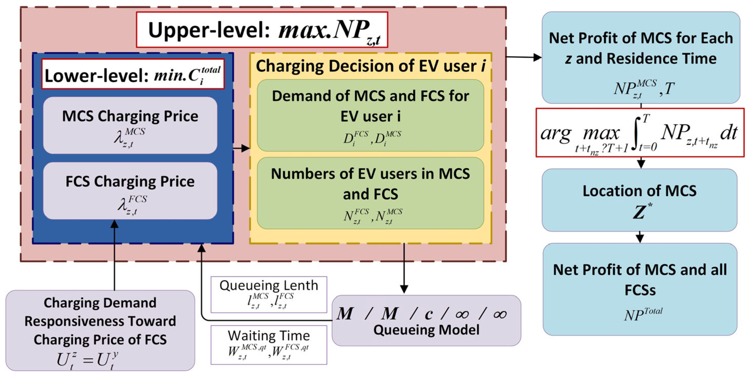
In this paper, a bi-level optimization model is proposed to address the dynamic location optimization of MCSs. The model integrates the charging decisions from the EV user side with the perspective of investor interests, aiming to maximize returns for investors, which can be represented in Figure 1.

The FCS charging price at location z, which has already been determined, can be input simultaneously with the initial MCS charging price into the lower level’s optimization algorithm aimed at minimizing EV user costs, thereby obtaining the optimal charging decision for EV users. The method of determining the queuing time and other parameters of FCSs can serve as a reference for MCSs. The EV user charging decision involves two key aspects: firstly, determining the charging capacity required by EV users when using either FCSs or MCSs, which helps derive the charging demand for both FCSs and MCSs; secondly, deciding whether to use FCSs or MCSs for charging, thus determining the number of EV users utilizing different methods. The access travel burden of EV users is treated according to the candidate-node structure of the charging network. In this study, the MCS can only be deployed at candidate nodes associated with existing FCS locations. Therefore, when an EV user compares MCSs and FCSs at the same candidate node, the access distance, access travel time, and access energy consumption are identical for the two charging modes and do not change their relative choice. The lower-level user decision, therefore, focuses on the cost components that differ between MCSs and FCSs, including charging price, queuing time, charging duration, and user-specific waiting-cost coefficients. For comparisons among different candidate nodes, spatial accessibility is represented by the road network distance matrix used in the siting process. A full dynamic traffic assignment model is outside the scope of this study. The queue length and waiting time for FCSs and MCSs are determined by the M/M/c/∞/∞ queuing theory.

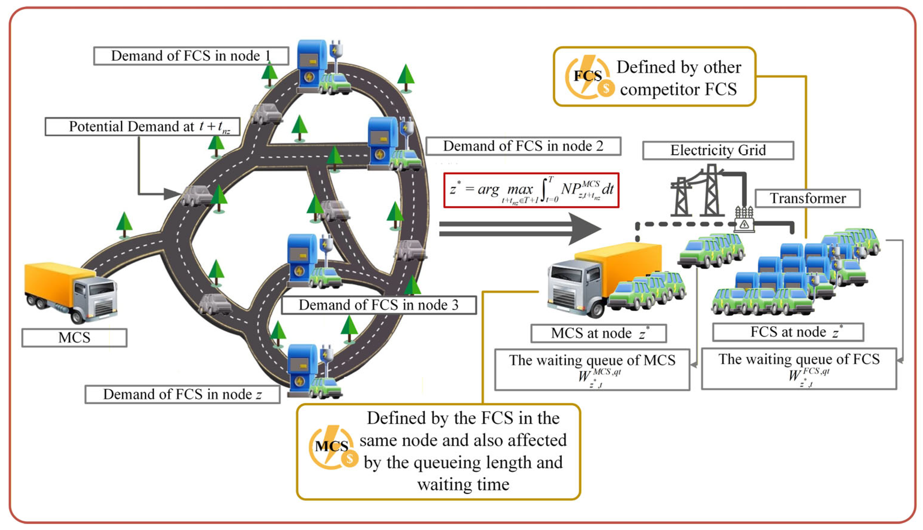
The parameters of the upper optimization model are determined based on the outcomes from the lower optimization model. Unlike conventional optimization models that solely focus on maximizing MCS profits, the newly proposed model integrates FCSs into the optimization process, not as a competitor but as a synergistic component, as shown in Figure 2. The objective is to maximize the combined net profit of FCSs and MCSs, thereby determining the optimal charging price set by MCSs. The corresponding MCS optimal charging price is then input into the lower-level optimization as a parameter. This iterative process continues until the total net profit at location z is maximized, ultimately yielding the optimal charging price set by MCSs and the charging demands for both FCSs and MCSs.

At the same time, upper-level optimization involves optimizing all locations at five-minute time intervals. By comparing the total net profit of MCSs and FCSs across all locations z ∈ Z at the same time, the location with the highest net profit is selected as the next-time node for MCSs. Subsequently, the residence time of MCSs is determined, thereby establishing the optimal dynamic location planning and scheduling for MCSs.

3. Conventional Dynamic Optimization Model

3.1. The Optimal Siting of Mobile Charging Stations

In conventional models, an MCS is typically allocated to a fixed FCS as a supplementary charging resource. The selection process evaluates multiple FCS locations and identifies the one with the highest aggregated daily demand.

$$z^{*}=\mathit{arg}\underset{z\in Z}{\mathit{max}}{\int }_{t=0}^{24}{D}_{z,t} dt$$

(1)

where $D_{z,t}$ denotes the total demand of EV user $i$ in node $z$, $z^{*}$ is the optimal node for the MCS, as it has the highest total adjusted demand among all nodes, and the candidate site for this node is the location of the existing FCS.

3.2. Distribution of Charging Demand Between MCSs and FCSs

EV users plan their charging modes by weighing the costs associated with waiting time and charging fees. According to the stochastic utility theory [28], the probability of different behaviors among EV users can be quantified, enabling the estimation of the spatiotemporal distribution of charging demand for both MCSs and FCSs.

$$C_{z,i}^{MCS}={\mathsf{\lambda }}_{\mathrm{z},\mathrm{t}}^{\mathrm{M}\mathrm{C}\mathrm{S}}\ast D_{z,i}+{\varpi }_i^{wc}\ast (W_z^{MCS,qt}+{\tau }_m({SOC}_i^{int},{SOC}_i^{final}\left)\right), z\in z^{*}$$

(2)

$$C_{z,i}^{FCS}={\mathsf{\lambda }}_{\mathrm{z},\mathrm{t}}^{\mathrm{F}\mathrm{C}\mathrm{S}}\ast D_{z,i}+{\varpi }_i^{wc}\ast (W_z^{FCS,qt}+{\tau }_f({SOC}_i^{int},{SOC}_i^{final}\left)\right), z\in z^{*}$$

(3)

where $C_{z,i}^{MCS}$ represents the total cost of EV user $i$ by using MCSs in node $z$; ${\mathsf{\lambda }}_{\mathrm{z},\mathrm{t}}^{\mathrm{M}\mathrm{C}\mathrm{S}}$ represents the electricity price of MCSs at node $z$ at time $t$; ${\varpi }_i^{wc}$ is the penalty coefficient that quantifies the monetary value equivalent of EV user $i$’s waiting time; $W_z^{MCS,qt}$ and $W_z^{FCS,qt}$ are the average queuing time for EV users by using MCSs and FCSs in node $z,$ respectively; ${\tau }_m\left(x,y\right)$ and ${\tau }_f(x,y)$ are the time required for an EV user to charge the battery from $x$ to $y$ by using MCSs and FCSs; and $D_{z,i}$ is the charging capacity of EV $i$ at node $z$. It represents the amount of energy required for the EV user to reach the target SOC. In this study, “charging demand” refers to energy demand, rather than the number of EVs or instantaneous charging power. The user cost expressions are used to evaluate the generalized charging costs of MCSs and FCSs. The cost-based selection probabilities are then calculated and used to allocate the required charging energy between the two charging modes.

Based on the generalized costs in Equations (2) and (3), the selection probabilities of EV user $i$ for MCSs and FCSs can be obtained. Equations (4) and (5) describe the probability that EV user $i$ selects MCSs and FCSs, respectively. Since the user’s choice is cost-oriented, a lower generalized cost produces a higher selection probability. These probabilities are later used to divide the required charging energy of each EV user between MCSs and FCSs.

$$\mathit{Pr}\left\{selecting MCS in node z^{*}\right\}={\displaystyle \frac{e^{C_{z,i}^{FCS}}}{e^{C_{z,i}^{MCS}}+e^{C_{z,i}^{FCS}}}}, z\in z^{*}$$

(4)

$$\mathit{Pr}\left\{selecting FCS in node z^{*}\right\}={\displaystyle \frac{e^{C_{z,i}^{MCS}}}{e^{C_{z,i}^{MCS}}+e^{C_{z,i}^{FCS}}}}, z\in z^{*}$$

(5)

$$\mathit{Pr}\left\{selecting MCS in node z^{*}\right\}+\mathit{Pr}\left\{selecting FCS in node z^{*}\right\}=1$$

(6)

After the selection probabilities are obtained, the required charging energy of EV user $i$ is allocated between MCSs and FCSs. The expected charging energy demand assigned to each charging mode is calculated as follows:

$$\begin{gathered} D_i^{MCS}=D_{z,i}\ast \mathrm{Pr}\left\{selecting MCS in node z^{*}\right\}, \\ {D}_i^{FCS}=D_{z,i}\ast \mathit{Pr}\left\{selecting FCS in node z^{*}\right\} \end{gathered}$$

(7)

where $D_{z,i}^{MCS}$ and $D_{z,i}^{FCS}$ denote the expected charging energy demand of EV $i$ allocated to MCSs and FCSs at node $z$, respectively; and $D_{z,i}$ is the total required charging energy of EV user $i$. The aggregate MCS and FCS demands at node $z$ can be obtained by summing $D_{z,i}^{MCS}$ and $D_{z,i}^{FCS}$ over all EV users assigned to that node, which can be expressed as $D_{z,i}^{MCS}+D_{z,i}^{FCS}=D_{z,i}$.

3.3. Profitability Assessment Model

With the MCS selecting z^* as the location, the FCS originally positioned at z^* will experience a redistribution of its charging demand. Consequently, both the FCS’s demand and net profit require readjustment.

For MCSs, the net profit in node $z$ can be expressed as:

$${maxNP}_z^{MCS}=D_z^{MCS}\ast {\lambda }_z^{MCS}-C_z^{MCS}, z\in z^{*}$$

(8)

where $D_z^{MCS}$ is the total demand of MCSs in node z; ${\lambda }_z^{MCS}$ denotes the charging price of MCSs in node $z$; and $C_z^{MCS}$ is the total cost of MCSs in node $z$.

The total net profit of all FCSs and MCSs owned by the investor using the conventional model can be shown as follows:

$$N{P}^{con}={NP}_z^{MCS}+{\displaystyle {\sum }_{t=0}^{24}}({\sum }_{z\in Z\backslash \left\{z^{*}\right\}}{NP}_{z,t}^{FCS}+{\sum }_{z\in z^{*}}{NP}_{z,t}^{FCS})$$

(9)

where ${NP}_{z,t}^{FCS}$ is the net profit of FCSs in node $z$.

4. Charging Demand Responsiveness Toward the Charging Price of FCS

In the context of the study, $z$ and $y$ are the locations of the charging stations. Prior to the introduction of MCSs, only FCSs were present at both $z$ and $y$. Location z is considered a potential candidate for MCS deployment, while location y serves as a competitor to $z$. The charging price at FCS node $y$ is defined as a known parameter. The pricing strategy for FCSs at location $z$ comprises two components. First, we need to establish an indifferent price between $z$ and $y$, which means the charging cost at $z$ and $y$ becomes irrelevant to their choice of charging station for EV users when $z$ adopts this indifferent price. Specifically, both $y$ and $z$ would be equal choices for EV users, with no preference given to either based on price.

$$U_t^z=-{\varpi }^{wc}\ast W_z^{FCS,qt}-{\lambda }_t^{z, FCS}\ast D_t, U_t^y=-{\varpi }^{wc}\ast W_y^{qt}-{\lambda }_t^y\ast D_t$$

(10)

where $U_t^z$ and $U_t^y$ represent the utility values for EV users selecting FCSs in node $z$ and node $y,$ respectively; $W_y^{qt}$ are the average queuing time for EV users in node $y$; ${\lambda }_t^{z, FCS}$ is the competitive charging price of FCSs in node $z$ at time $t$ regarding the demand; ${\lambda }_t^y$ is the charging price in node $y$; and $D_t$ is the total competitive demand of EV users.

Given that $U_t^z={\displaystyle \frac{1}{\left|Y\right|}}\sum _{y\in Y}{U}_t^y$, an expression for the price difference $∆{\lambda }_t^{\ast }$ can be derived by combining the equations of $U_t^z$ and $U_t^y$.

$$-{\varpi }^{wc}\ast W_z^{FCS,qt}-{\lambda }_t^{z, FCS}\ast D_t-{\displaystyle \frac{1}{\left|Y\right|}}{\sum }_{y\in Y}(-{\varpi }^{wc}\ast W_y^{qt}-{\lambda }_t^y\ast D_t)=0$$

(11)

$$-{\varpi }^{wc}\ast (W_z^{FCS,qt}-{\displaystyle \frac{\sum _{y\in Y}{W}_y^{qt}}{\left|Y\right|}})-D_t\ast \left({\lambda }_t^{z, FCS}-{\displaystyle \frac{\sum _{y\in Y}{\lambda }_t^y}{\left|Y\right|}}\right)=0$$

(12)

$$∆{\lambda }_t^{*}={\lambda }_t^{z, FCS}-\overline{{\lambda }_t^y}={\displaystyle \frac{-{\varpi }^{wc}\ast \left(W_z^{FCS,qt}-\overline{W_y^{qt}}\right)}{D_t}}$$

(13)

Then, based on the specified charging price of FCSs at node $y$ and Equation (13), the indifference price ${\lambda }_t^{z\ast }$ can be determined by Equation (14).

$${\lambda }_t^{z*}={\lambda }_t^y+∆{\lambda }_t^{*}$$

(14)

After being determined through Equations (10)–(14), the indifference price can be treated as a known parameter, facilitating the analysis of the responsiveness of competitive demand to charging prices. To characterize the distribution of competitive demand under varying charging prices, an exponential distribution model can be incorporated into Equation (15). This model effectively captures the relationship between the charging price of FCSs at node $z$ and the probability of competitive demand, thereby providing a theoretical foundation for subsequent pricing optimization.

$$P_r^{com}={\varpi }_t^{dem}\ast e^{-{\varpi }_t^{dem}*{\lambda }_{z,t}^{FCS}}$$

(15)

where $P_r^{com}$ represents the proportion of competitive demand that $z$ can attract; ${\varpi }_t^{dem}$ denotes the demand response coefficient at time t, which describes the EV user’s sensitivity to price changes; and ${\lambda }_{z,t}^{FCS}$ is the charging price of FCSs in node z at time t.

To ensure that there is no competition between all nodes $y\in Y$ and $z$, it can be deduced that $P_r^{com}={\displaystyle \frac{1}{\left|\mathrm{Y}\right|}}$. Subsequently, substituting this result into Equation (15) yields Equation (16).

$$f\left({\varpi }_t^{dem}\right)={\varpi }_t^{dem}\ast e^{-{\varpi }_t^{dem}*{\lambda }_t^{z*}}-{\displaystyle \frac{1}{\left|\mathrm{Y}\right|}}$$

(16)

Assume that $f\left({\varpi }_t^{dem}\right)$ is $d+1$ times a continuously differentiable function, then ${\varpi }_{i+1,t}^{dem}$, the demand response coefficient at iteration $d+1$ at time $t$, can be shown as Equation (17) by applying the Householder method.

$${\varpi }_{d+1,t}^{dem}={\varpi }_{i,t}^{dem}+d{\displaystyle \frac{(1/{f)}^{d-1}({\varpi }_{i,t}^{dem})}{(1/{f)}^d({\varpi }_{i,t}^{dem})}}$$

(17)

Because $d$ in $f\left({\varpi }_t^{dem}\right)$ is 1, it can be seen as Newton’s method:

$$\begin{gathered} {\varpi }_{d+1,t}^{dem}={\varpi }_{i,t}^{dem}+d{\displaystyle \frac{(1/{f)}^{d-1}({\varpi }_{d,t}^{dem})}{(1/{f)}^d({\varpi }_{d,t}^{dem})}}={\varpi }_{i,t}^{dem}+{\displaystyle \frac{1}{f\left({\varpi }_t^{dem}\right)}}\ast {\left({\displaystyle \frac{\frac{df\left({\varpi }_{d,t}^{dem}\right)}{d{\varpi }_t^{dem}}}{f{\left({\varpi }_{d,t}^{dem}\right)}^2}}\right)}^{-1} \\ ={\varpi }_{d,t}^{dem}-{\displaystyle \frac{d{\varpi }_t^{dem}}{df\left({\varpi }_{d,t}^{dem}\right)}}\ast f\left({\varpi }_{d,t}^{dem}\right) \end{gathered}$$

(18)

$${\varpi }_{d+1,t}^{dem}={\varpi }_{d,t}^{dem}-{\displaystyle \frac{d{\varpi }_t^{dem}}{df\left({\varpi }_{d,t}^{dem}\right)}}\ast f\left({\varpi }_{d,t}^{dem}\right)$$

(19)

5. Proposed Charging Demand and EV User Behavior Interaction

5.1. Queueing Model

When EV users enter the node $z$ to charge, the number of EV users arriving may exceed the number of available chargers, necessitating consideration of queuing dynamics. The queuing model employed is $M/M/c/\infty /\infty$, where the first M denotes the arrival rate of EV users; another M represents the service rate for charging; c indicates the number of parallel chargers at node $z$ [29]. The relationship between the relevant parameters is presented in Equations (20)–(26).

$$W_{t,z}^{FCS,qt}={\displaystyle \frac{l_{z,t}^{FCS}}{{\epsilon }_{z,t}^{arr}}},t\in T$$

(20)

where $l_{z,t}^{FCS}$ represents the queue length of FCSs in node $z$ at time t, and ${\epsilon }_{z,t}^{arr}$ represents the arrival rate of EV users at time $t$ in $z$.

$${\tau }_f\left({SOC}_i^{int},{SOC}_i^{final}\right)={\displaystyle \frac{{SOC}_i^{final}-{SOC}_i^{int}}{r^{FCS}}},i\in F$$

(21)

where $r^{FCS}$ denotes the charging rate of FCS.

$${\epsilon }_{z,t}^{uti}={\displaystyle \frac{{\epsilon }_{z,t}^{arr}}{{\kappa }^{FCS}\ast {\epsilon }_{z,t}^{ser}}},i\in F$$

(22)

$${\epsilon }_{z,t}^{arr}={\displaystyle \frac{N_{z,t}^{FCS}-1}{{\displaystyle {\sum }_i^{N_{z,t}^{FCS}}}∆t_i}},i\in F$$

(23)

$${\epsilon }_{z,t}^{ser}={\displaystyle \frac{N_{z,t}^{FCS}-1}{{\displaystyle {\sum }_i^{N_{z,t}^{FCS}}}{\tau }_f\left({SOC}_i^{int},E_i^{FCS}\right)}},i\in F$$

(24)

$$l_{z,t}^{FCS}={\displaystyle {\sum }_{n={\kappa }^{FCS}+1}^{\infty }}\left(n-{\kappa }^{FCS}\right)\ast P_{rt,z}^{chr}={\displaystyle \frac{{\left({\kappa }^{FCS}\ast {\epsilon }_{z,t}^{uti}\right)}^{{\kappa }^{FCS}}\ast {\epsilon }_{z,t}^{uti}}{{\kappa }^{FCS}!\ast {\left(1-{\epsilon }_{z,t}^{uti}\right)}^2}}\ast P_{rt,z}^{chr},t\in T$$

(25)

where ${\epsilon }_{z,t}^{uti}$ represents the utility rate of EV users at time $t$ in node $z$; ${\kappa }_z^{FCS}$ denotes the chargers’ number of FCSs in node $z$; and $P_{rt,z}^{chr}$ denotes the state probability in node $z$, which can also be interpreted as the probability that all chargers are standing by.

$$P_{rt,z}^{chr}=[{\displaystyle {\sum }_{k=0}^{{\kappa }^{FCS}-1}}{\displaystyle \frac{1}{k!}}\ast {\left({\displaystyle \frac{{\epsilon }_{z,t}^{arr}}{{\epsilon }_{z,t}^{ser}}}\right)}^k+{\displaystyle \frac{1}{{\kappa }^{FCS}!}}\ast {\displaystyle \frac{1}{1-{\epsilon }_{z,t}^{uti}}}\ast {\left({\displaystyle \frac{{\epsilon }_{z,t}^{arr}}{{\epsilon }_{z,t}^{ser}}}\right)}^{{\kappa }^{FCS}}{]}^{-1},t\in T$$

(26)

where ${\epsilon }_{z,t}^{ser}$ represents the service rate of EV users at time $t$ in node $z$.

The mathematical formulations collectively describe the operational characteristics of FCSs in different states, encompassing the charging duration for EV users, utility rate, arrival rate, service rate, queue length and state probability, Firstly, the charging duration ${\tau }_f\left({SOC}_i^{int},{SOC}_i^{final}\right)$ at an FCS is dictated by the initial state-of-charge (SOC), target SOC, and charging rate, which in turn affects the overall service capacity and queuing dynamics of the station. Equation (22) is determined by the arrival rate ${\epsilon }_{z,t}^{arr}$ and service rate ${\epsilon }_{z,t}^{ser}$, reflecting the level of congestion at the charging station at a given time. Additionally, the arrival rate in Equation (23) is calculated based on the total number of EVs entering the station and their arrival intervals, while Equation (24) is influenced by the charging demand, SOC variations, and charging power. Furthermore, the queue length $l_{z,t}^{FCS}$ in Equation (25) is determined by aggregating the number of EVs exceeding the maximum charging capacity, thereby quantifying the queuing burden of the station. Lastly, the state probability $P_{rt,z}^{chr}$ represents the likelihood that all chargers at the station remain idle, a crucial parameter for assessing whether an EV user can access immediate charging upon arrival.

5.2. Lower Level: Cost-Optimized Demand Allocation for MCSs and FCSs from a Customer Perspective

Assuming that every EV user acts as a rational decision maker, they will aim to minimize costs for both FCSs and MCSs in node $z$, which constitutes the lower-level optimization objective. It involves comparing the prices and queue times of FCSs and MCSs during the order confirmation process [30]. Given that FCSs in node $z$ may experience long or unpredictable waiting times, EV users will determine the amount of charging at FCSs and MCSs based on their preference, quantified by a penalty factor ${\varpi }^{wc}$ that represents the monetary equivalent of waiting time. Due to the unpredictability associated with FCS, an additional cost parameter $\phi$ is introduced to account for potential extra expenses incurred by EV user $i$ when using FCS. Since the penalty coefficient ${\varpi }^{wc}$ is strongly correlated with the income of EV users, conventional calculation methods have employed the production approach (PA) [31] and the average income approach (AIA) [24,32]. Building on this foundation, this paper further incorporates the cumulative queuing time of EV users and integrates a psychological time value growth factor into the calculation of the time penalty coefficient ${\varpi }^{wc}$.

It should be noted that the access cost of EV users is node-based in the proposed formulation. Since MCS deployment is restricted to the same candidate nodes as existing FCS, the travel distance from an EV user to the selected node is the same whether the user chooses MCSs or FCSs at that node. As a result, the access travel time and access energy consumption are common terms in the MCS-FCS comparison at the same node and are not separately included as independent decision variables in the lower-level optimization. This treatment avoids the double-counting of identical access costs while preserving the relative cost comparison between MCSs and FCSs.

$$\begin{gathered} min. C_i^{total}(x_i^{MCS}, D_i^{MCS}, x_i^{FCS}, D_i^{FCS}){=x}_i^{MCS}\ast ({\varpi }_i^{wc}\ast \left({\tau }_m\left({SOC}_i^{int},D_i^{MCS}\right)+W_i^{qt,MCS}\right)+ \\ {D}_i^{MCS}\ast {\lambda }_{z,t}^{MCS})+x_i^{FCS}\ast ({\lambda }_{z,t}^{FCS}\ast D_i^{FCS}+{\varpi }_i^{wc}\ast {\tau }_f({SOC}_i^{int}+D_i^{MCS},D_i^{FCS})+W_i^{qt,FCS})+\phi ) \end{gathered}$$

(27)

$$s.t. {\varpi }_i^{wc}={ \gamma }_t\ast {\displaystyle \frac{I_i}{\overline{H_i}}}$$

(28)

$$x_i^{MCS}\ast D_i\ge D_i^{MCS}$$

(29)

$$x_i^{FCS}\ast D_i\ge D_i^{FCS}$$

(30)

$$D_i^{MCS},D_i^{FCS}\ge 0$$

(31)

$${\sum }_{i\in M}{D}_i^{MCS}+{\sum }_{i\in F}{D}_i^{FCS}=D_z^{adj}$$

(32)

$$x_i^{FCS},x_i^{MCS}\in \left\{\mathrm{0,1}\right\} and x_i^{FCS}+x_i^{MCS}\ne 0$$

(33)

where in Equation (27), $C_i^{total}(x_i^{MCS},D_i^{MCS},x_i^{FCS},D_i^{FCS})$ represents the total charging cost of EV user $i$, which is determined by $x_i^{MCS},D_i^{MCS},x_i^{FCS},D_i^{FCS}$. The first part represents the time cost and charging cost incurred when EV user $i$ chooses MCSs, while the second part corresponds to the time cost, charging cost, and additional expenses associated with selecting FCS. The binary variables $x_i^{MCS}$ and $x_i^{FCS}$ represent the decisions of EV users regarding the use of MCSs and FCSs for charging, where $x_i^{MCS}:\{x_i^{MCS}:i\in I\}$ and $x_i^{FCS}:\{x_i^{FCS}:i\in I\}$. Specifically, when $x_i^{MCS}=1$ or $x_i^{FCS}=1$, it indicates that EV user i has chosen to use MCSs or FCSs for charging, respectively. Conversely, when $x_i^{MCS}=0$ or $x_i^{FCS}=0$, it signifies that EV user $i$ has decided not to use MCSs or FCSs. $D_i^{MCS}$ and $D_i^{FCS}$ denote the final charging demand of EV user $i$ in MCSs and FCSs, respectively. In Equation (28), $I_i$ represents the monthly income obtained by EV user $i$ through income distribution; ${\gamma }_t$ denotes the temporal value growth coefficient of electric vehicle user i’s psychological perception; and $\overline{H_i}$ is the average number of working hours of residents per month. In Equation (29), $D_i$ represents the required charging amount of EV user $i$.

Since the node z supports two charging modes, FCSs and MCSs, it is possible for EV user $i$ to utilize both modes simultaneously. The queue length and waiting time for MCSs are shorter than those for FCS, indicating that the opportunity cost of choosing MCSs is lower for EV user $i$. Consequently, a higher proportion of EV users are likely to choose MCSs. However, since an MCS incurs higher costs compared to an FCS, its pricing will be correspondingly higher. Assuming all EV users act rationally, as battery power increases, the advantages of mobile charging diminish due to decreasing charging rates. Therefore, EV users may initially opt for mobile charging and subsequently switch to fixed charging once a certain charge level is reached. This paper does not consider scenarios where EV users exclusively use fixed charging because the selection process for MCS locations already ensures that chosen locations are oversaturated. The criteria for selecting MCS moving positions will be detailed in Section 6. When both charging modes are utilized, the charging cost for EV user $i$ at location z can be reformulated as follows:

$$\underset{E_i^{\mathit{MCS}}}{\min }.C_i^{EV}\left(E_i^{MCS}\right)=D_i^{MCS}\ast {\lambda }_{z,t}^{MCS}+{\varpi }_i^{wc}\ast (W_i^{qt,MCS}+W_i^{qt,FCS})+{\lambda }_{z,t}^{FCS}\ast D_i+ϵ+\chi (E_i^{MCS})$$

(34)

$$s.t.D_i^{MCS}\in \left(0,D_i\right)$$

(35)

$$\chi \left(E_i^{MCS}\right)={\varpi }_i^{wc}\ast {\tau }_m\left({SOC}_i^{int},E_i^{MCS}\right)-{\lambda }_{z,t}^{FCS}\ast D_i^{MCS}+{\varpi }_i^{wc}\ast {\tau }_f({SOC}_i^{int}+E_i^{MCS},D_i-D_i^{MCS})$$

(36)

$$N_{z,t}^{FCS}=\sum x_i^{FCS}$$

(37)

where in Equation (36), $\chi \left(E_i^{MCS}\right)$ is an intermediate variable that integrates the influence factors of MCSs and FCSs, enabling EV users to optimize their charging options based on price, waiting time, and other relevant factors to minimize their overall charging costs. The primary factors influencing $\chi \left(E_i^{MCS}\right)$ include the availability of MCS charging stations, the pricing of MCS charging services, and the wait times and availability of FCS. When $\chi \left(E_i^{MCS}\right)$ > 0, it signifies that the MCS charging station has a high load, extended waiting times, or higher costs, leading customers to reduce their reliance on MCS charging ($E_i^{MCS})$. Conversely, when $\chi \left(E_i^{MCS}\right)$ < 0, it indicates that the MCS charging station has a lower load, offering additional benefits such as shorter waiting times or reduced charging costs, encouraging customers to increase $E_i^{MCS}$.

6. Proposed Profit-Driven Dynamic Siting of MCSs

6.1. Upper Level: Dynamic Siting of MCSs

The upper level is to maximize the net profit of MCSs, which serves as the criterion for determining its optimal position in Equation (46). Based on this principle, the total net profit for both FCS and MCS ${NP}^{total}$ after implementing the new location planning can be expressed.

$$\underset{t+t_{yz}\in T+1}{max}{NP}^{total}={\sum }_{z\in Z^{\ast }}{\sum }_{t\in T}{NP}_{z,t}^{MCS}+{\sum }_{z\in Z\backslash \left\{Z^{\ast }\right\}}{\displaystyle {\sum }_{t=0}^{24}}{NP}_{z,t}^{FCS}+{\sum }_{z\in Z^{\ast }}{\sum }_{t\in T}{NP}_{z,t}^{FCS,adj}$$

(38)

$$s.t. {NP}_{z,t+t_{yz}}^{MCS}=D_{t+t_{yz}}^{MCS}\ast {\lambda }_{z,t+t_{yz}}^{MCS}-C_{z,t+t_{yz}}^{MCS},t+t_{yz}\in T+1$$

(39)

$$t_{yz}={\displaystyle \frac{d_{yz}}{v}}$$

(40)

where ${\lambda }_{z,t}^{MCS}$ represents the charging price of MCSs in node $z$ at time $t$; $C_{z,t}^{MCS}$ denotes the total cost of MCSs in node z at time t; $t_{yz}$ is the time duration an MCS moves from node y to node $z$; $d_{yz}$ is the distance from node y to node $z$; and $v$ is the average speed of MCS. The net profit of FCSs and MCSs Equation (38) consists of three parts: the total profit of an MCS at its optimal location $z\in Z^{\ast }$, the profit of FCS locations not selected by MCSs, and the profit of FCSs influenced by MCSs at specific times and places.

In Equation (41), the cost of MCSs can be categorized into three parts: investment cost, operating cost, and variable cost.

$$C_{z,t}^{MCS}={\displaystyle {\sum }_{m=1}^3}{o}_{m,t}\ast {\displaystyle \frac{1-\mathit{exp}\left(-{\sigma }^{dis}\ast {\rho }_m\right)}{{\sigma }^{dis}\ast {\rho }_m}}$$

(41)

$$o_{1,t}=(C^{lb}\ast {\displaystyle \frac{{\zeta }^{wf}\ast {\sum }_{i\in M}{D}_z^{MCS}}{{\zeta }^{dod}}}+C^{ct})\ast {\displaystyle \frac{{\sigma }^{dep}\ast {\left(1+{\sigma }^{dep}\right)}^L}{{\left(1+{\sigma }^{dep}\right)}^L-1}}\ast t,t\in T$$

(42)

$$o_{2,t}={\sum }_{i\in M}{D}_i^{MCS}\ast C^{op}$$

(43)

$$o_{3,t}={\lambda }^{grid}\ast ({\eta }^{disc}\ast {\zeta }^{dod}\ast {\sum }_{i\in M}{D}_i^{MCS}+d_{yz}\ast \overline{E^{MCS}}\ast {\eta }^{chr})$$

(44)

$${\zeta }^{wf}\propto {\displaystyle \frac{{\sum }_{i\in M}{D}_i^{MCS}\ast {\epsilon }_{z,t}^{uti}}{{\kappa }^{MCS}}}\ast \left(1+{\displaystyle \frac{l_{z,t}^{MCS}}{N_{z,t}^{MCS}}}\right)$$

(45)

where ${\sigma }^{dis}$ denotes the discount rate which is used to convert the value of future costs to the current cost, and ${\rho }_m$ is the cost adjustment factor of different costs. $C^{lb}$, $C^{ct}$, and $C^{op}$ represent the cost of lithium-ion battery packs, the cost of MCSs’ chargers, trucks, and containers, and the unit operational cost, respectively. ${\zeta }^{wf}$, ${\zeta }^{dod}$, and ${\sigma }^{dep}$ are the weighting coefficients of the lithium-ion battery pack, depth of discharge with round-trip efficiency, aging-induced degradation, and the depreciation rate, respectively. $L$ represents the lifespan; ${\lambda }^{grid}$ denotes the electricity purchase price for MCSs from the grid; ${\eta }^{chr}$ and ${\eta }^{disc}$ are the charging efficiency of MCSs and the efficiency parameter corresponding to the energy loss, respectively; and $\overline{E^{MCS}}$ is the average energy consumption per kilometer for MCSs.

The grid electricity cost in Equation (44) is associated with the energy required to recharge the onboard MCS battery and to compensate for the energy consumed during relocation. Therefore, the grid purchase cost should be interpreted together with the MCS battery energy state rather than as an independent cost term. To ensure that the obtained MCS dispatch trajectory is physically implementable, the onboard battery SOC evolution, charging/discharging limits, relocation energy consumption, and driving-range feasibility are verified in the following subsection.

The optimal location is determined by comparing the overall net profits of FCSs and MCSs across various locations during an identical time frame.

$$z^{*}=\mathit{arg}\underset{\mathit{t}+t_{\mathit{yz}}\in T+1}{\mathit{max}}{\int }_{t=0}^T{NP}^{total} dt$$

(46)

The dispatch trajectory selected by Equation (46) is further checked against the onboard battery energy feasibility constraints described in the following subsection, so that MCS relocation, EV charging service, and inter-station movement remain physically implementable over the full-day horizon. The relocation time between two candidate nodes is calculated from the road network distance and the average travel speed of the MCS. During the relocation interval, the MCS is not available for EV charging service. Therefore, the relocation process affects both the service availability of the MCS and its onboard battery energy state, while the relocation energy consumption is further checked by the SOC feasibility constraints in Section 6.2.

6.2. MCS Onboard Battery Feasibility Verification

The MCS is equipped with an onboard battery energy storage system. Although the proposed bi-level model determines the MCS siting, pricing, and service demand from the economic and user-choice perspectives, the obtained MCS dispatch trajectory should also satisfy physical battery feasibility over the full-day horizon. Therefore, an onboard battery feasibility verification layer is introduced to track the MCS energy state across time intervals, service operation, and inter-station relocation.

The corresponding SOC can be defined as Equation (47), and the onboard battery energy should remain within the allowable SOC range as shown in Equation (48):

$$SO{C}_t^{MCS}={\displaystyle \frac{B_t^{MCS}}{{\overline{B}}^{MCS}}},t\in T$$

(47)

$${\underset{\_}{SOC}}^{MCS}{\overline{B}}^{MCS}\le B_t^{MCS}\le {\overline{SOC}}^{MCS}{\overline{B}}^{MCS}$$

(48)

where $B_t^{MCS}$ denote the onboard battery energy of the MCS at time interval t, ${\overline{B}}^{MCS}$ is the rated onboard battery capacity; ${\underset{\_}{SOC}}^{MCS}$ and ${\overline{SOC}}^{MCS}$ represent the minimum and maximum allowable SOC levels of the MCS battery.

The charging and discharging powers of the MCS are limited by:

$$0\le P_t^{ch,MCS}\le {\overline{P}}_t^{ch,MCS},t\in T$$

(49)

$$0\le P_t^{dis,MCS}\le {\overline{P}}^{dis,MCS},t\in T$$

(50)

where $P_t^{ch,MCS}$ is the charging power of the MCS battery when the MCS is connected to a grid-coupled charging node, and $P_t^{dis,MCS}$ is the discharging power used to serve the EV charging demand.

The discharging energy used for EV service is determined by the accepted MCS charging demand:

$$P_t^{dis,MCS}\Delta t={\sum }_{i\in M}{D}_{i,t}^{MCS},t\in T$$

(51)

When the MCS moves from node $y\to z$, the required driving energy is shown as:

$$B_{t+1}^{MCS} =B_t^{MCS} +{\eta }^{ch}{P}_t^{ch,MCS} \Delta t-{\displaystyle \frac{P_t^{dis,MCS}\Delta t}{{\eta }^{disc}}} --d_{yz}\overline{E^{MCS}}{u}_{yz,t},t\in T$$

(52)

where $u_{yz,t}$ is a binary relocation indicator. If the MCS moves from node $y$ to node $z$ during interval $t$, $u_{y,z,t}=1$; otherwise, $u_{y,z,t}=0$.

To ensure driving range feasibility, the MCS must have sufficient onboard energy before relocation:

$$B_t^{MCS}\ge d_{yz}\overline{E^{MCS}}{u}_{yz,t}+{\underset{¯}{SOC}}^{MCS}{\overline{B}}^{MCS}, y,z\in Z,t\in T$$

(53)

This condition prevents infeasible relocation decisions caused by insufficient onboard battery energy.

The location state of the MCS is described by

$${\sum }_{z\in Z}{a}_{z,t}^{MCS}=1,t\in T$$

(54)

where $a_{z,t}^{MCS}$ is a binary variable that equals 1 if the MCS is located at node $z$ during interval $t$, and 0 otherwise.

The relocation indicator is linked with the location state by Equation (55), and the initial and terminal battery energy levels are given by Equations (56) and (57).

$$u_{yz,t}\ge a_{y,t}^{MCS}+a_{z,t+1}^{MCS}-1,y,z\in Z,y\ne z,t\in T$$

(55)

$$B_0^{MCS} =B_{ini}^{MCS}$$

(56)

$$B_{\left|T\right|}^{MCS}\ge B_{end}^{MCS}$$

(57)

where $B_{ini}^{MCS}$ and $B_{end}^{MCS}$ are the required initial and terminal onboard battery energy levels. Through these equations, the full-day MCS dispatch trajectory can be checked against SOC limits, charging/discharging capability, relocation energy consumption, and inter-station energy continuity.

6.3. Power System Constraints

The MCS is modeled as a battery-supported mobile charging resource. When it is connected to a grid-coupled FCS, its battery recharging power is reflected as an additional local load. During EV service, the MCS supplies charging energy through its onboard battery, and the corresponding energy feasibility is checked by the SOC verification constraints in Section 6.2. Therefore, the operation of MCSs affects the distribution network mainly through the charging power required for battery replenishment and the additional service load at the coupled node. To capture these impacts, the power flow constraints are modified as follows.

$$P_{pq,t}+P_{q,t}-r_{pq}\ast {\displaystyle \frac{{P_{pq,t}}^2+{Q_{pq,t}}^2}{V_{q,t}^2}}={\sum }_{k\in K}{P}_{qk,t}+{\sum }_{i\in M\cup F}{D}_{i,t}\ast ({\tau }_m({SOC}_i^{int},D_i^{MCS})+{\tau }_f\left({SOC}_i^{int}+D_i^{MCS},D_i^{FCS}\right){)}^{-1}+P_{q,t}^{MCS}$$

(58)

$$Q_{pq,t}+Q_{q,t}-x_{pq}\ast {\displaystyle \frac{{P_{pq,t}}^2+{Q_{pq,t}}^2}{V_{q,t}^2}}={\sum }_{k\in K}{Q}_{qk,t}+Q_{q,t}^{MCS}$$

(59)

where the $P_{pq,t}$ and $Q_{pq,t}$ represent the active and reactive power flow from bus $p$ to bus $q$, respectively; $r_{pq}$ and $x_{pq}$ are the resistance and reactance from bus $p$ to bus $q$; $P_{q,t}^{MCS}$ and $Q_{q,t}^{MCS}$ are the active and reactive power demands of MCSs in bus $q$ at time t; $P_{q,t}$ and $Q_{q,t}$ are the active and reactive power flows generated by bus $q$ at time t before the MCSs join bus $q$; and $V_{q,t}$ is the voltage of bus $q$ at time $t$.

Equations (58) and (59) describe the active and reactive power balance within the grid. It ensures that the generation and consumption of active (reactive) power in the power system are in equilibrium, thereby preventing line overloading and maintaining voltage stability in the power system.

$$V_{q,t}^2-V_{p,t}^2=2\ast (r_{pq}\ast (P_{pq,t}+P_{q,t}^{MCS})+x_{pq}\ast (Q_{pq,t}+Q_{q,t}^{MCS}))-\left(r_{pq}^2+x_{pq}^2\right)\ast {\displaystyle \frac{{\left(P_{pq,t}+P_{q,t}^{MCS}\right)}^2+{\left(Q_{pq,t}+Q_{q,t}^{MCS}\right)}^2}{V_{q,t}^2}}$$

(60)

$$V_q^{min}\le V_{q,t}-{∆V}_{q,t}^{MCS}\le V_q^{max}$$

(61)

$${∆\mathrm{V}}_{\mathrm{q},\mathrm{t}}^{\mathrm{T}\mathrm{M}\mathrm{C}}=k_q\ast P_{q,t}^{MCS}+m_q\ast Q_{q,t}^{MCS}$$

(62)

$$\sqrt{{\left(P_{pq,t}+P_{q,t}^{MCS}\right)}^2+{\left(Q_{pq,t}+Q_{q,t}^{MCS}\right)}^2}\le S_{pq}^{max}$$

(63)

$${\sum }_{i\in M\cup F}{D}_{i,t}\ast ({\tau }_m\left({SOC}_i^{int},D_i^{MCS}\right)+{\tau }_f({SOC}_i^{int}+D_i^{MCS},D_i^{FCS}){)}^{-1}+P_{q,t}^{MCS}\le P_q^{FCS,max}$$

(64)

where $V_q^{\mathrm{m}\mathrm{i}\mathrm{n}}$ and ${\mathrm{V}}_{\mathrm{q}}^{\mathrm{m}\mathrm{a}\mathrm{x}}$ represent the lower and upper voltage limits at bus $q$; ${∆\mathrm{V}}_{\mathrm{q},\mathrm{t}}^{\mathrm{T}\mathrm{M}\mathrm{C}}$ denotes the voltage deviation induced by MCSs; $k_q$ and $m_q$ are the voltage sensitive to active and reactive power at bus $q$; $S_{pq}^{max}$ is the maximum line capacity between bus $p$ and bus $q$; and $P_q^{FCS,max}$ is the maximum permissible charging power of FCSs at bus $q$.

Equation (60) delineates the voltage relationship between adjacent buses. It ensures voltage stability and prevents both overvoltage and undervoltage conditions. When an MCS charges at an FCS, it occupies part of the FCS’s power capacity. Equation (64) ensures that the total charging power remains within the maximum permissible charging limit of the FCS.

7. Case Study

To address the complexity of the original nonlinear, non-convex bi-level optimization model, we implemented several techniques to enhance computational feasibility. We introduced Big-M, auxiliary variables, and applied piecewise linear approximation, converting problematic expressions into manageable structures for optimization. The bi-level problem was transformed into a single-level MPEC by embedding the KKT conditions of the lower-level problem into the upper-level objective. We then used the YALMIP toolbox with Gurobi as the primary solver for efficient processing of the transformed model.

7.1. Simulation Configuration

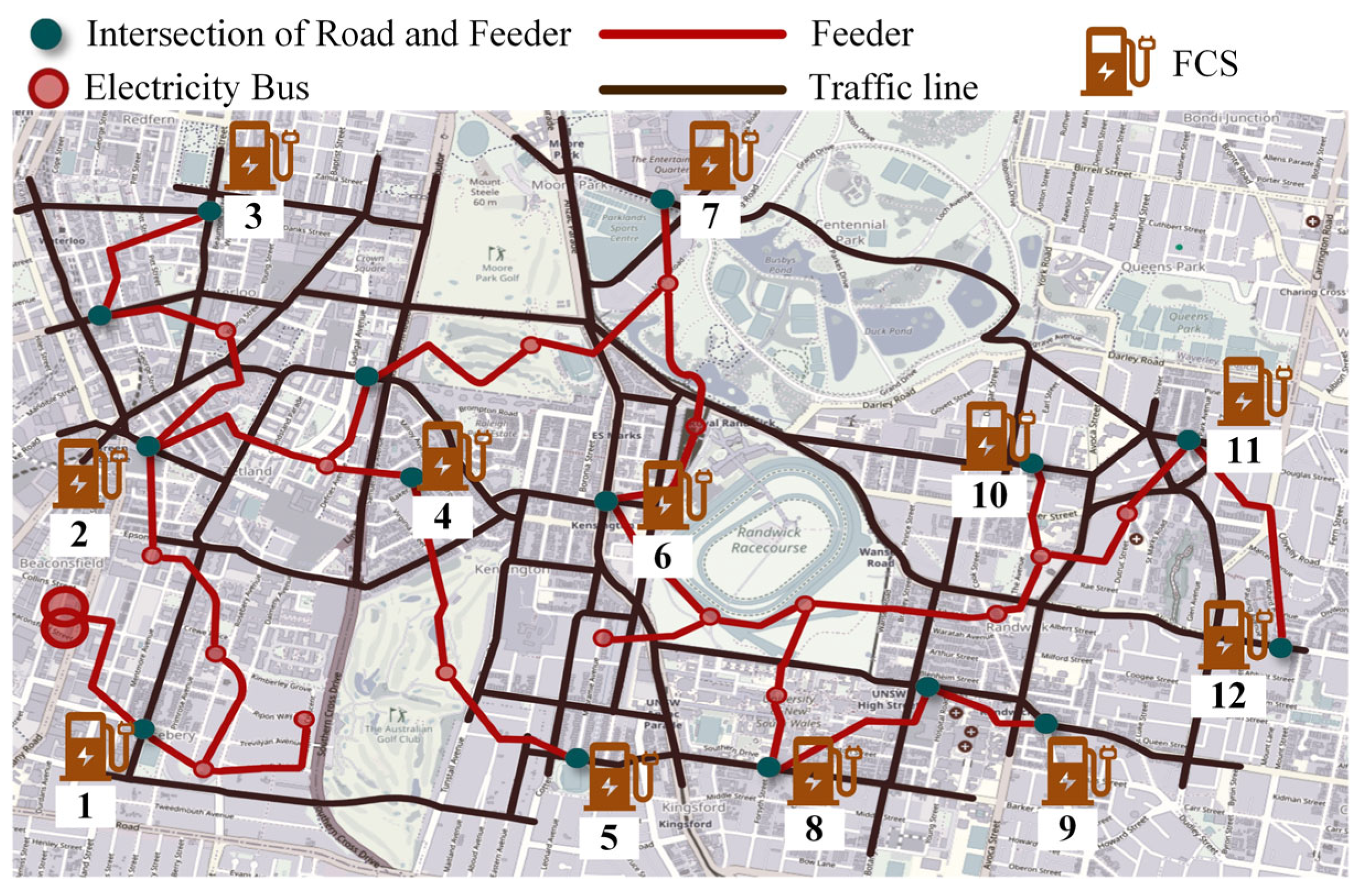
The proposed bi-level collaborative dynamic pricing optimization strategy is validated using the IEEE 33-bus distribution system coupled with an urban transportation network constructed from real geographic information in the southern region of Sydney, Australia. As illustrated in Figure 3, the studied road network contains 14 candidate road-power coupling nodes and 47 primary and secondary road links. Among these 14 candidate nodes, 12 nodes are equipped with investor-owned FCSs and are used as candidate locations for MCS deployment. The power distribution network includes a 110 kV substation, and the transportation and power distribution networks are coupled through the FCS nodes located at road intersections. The maximum inter-node distance in the road network distance matrix is approximately 8 km, indicating that the case study focuses on short-distance urban MCS relocation rather than intercity mobile charging operation.

Table 1. Main simulation settings for the coupled charging-service network.

Electric vehicle charging station parameters
Arrival rate (veh/5 min) (during active charging interval)	1.618–2.083	Maximum inter-node distance (km)	8
Electric vehicle parameters
Station-level original demand range (kWh/day)	4650–5770.5	Station-level Served charging energy (kWh/day)	4434.5–5255
Average SOC changing (%)	25.687	Average charging time (min)	23.824
MCS parameters		FCS parameters
Number of chargers	7	Number of chargers	20
Maximum power of each charger (kW)	85	Maximum power of each charger (kW)	32

summarizes the key simulation settings used in the case study. The charging-service capacity of each facility is determined by the number of parallel chargers and the maximum power of each charger. Each investor-owned FCS is equipped with 20 parallel chargers, and the maximum power of each FCS charger is 32 kW. The MCS is equipped with seven chargers, and the maximum power of each MCS charger is 85 kW. These parameters are used to calculate charging duration, service rate, station utilization, and queuing time in the M/M/c queuing model.

The arrival rate is reported for active charging intervals, during which EV arrivals occur at the candidate charging nodes. The arrival-time dataset contains 6370 EV charging requests over the 24 h simulation horizon. Since each arrival time corresponds to one EV charging request, the total number of EV charging requests is obtained by counting the station-level arrival-time entries. The station-level demand range represents the daily charging demand distributed across the investor-owned FCS nodes, while the station-level charging-energy range represents the daily charging energy served under the simulated operation. The maximum inter-node distance is obtained from the road network distance matrix and is used to characterize the spatial scale of MCS relocation.

In this study, the EV charging reservation information includes the initial SOC values and total charging demands of EV users, which are simulated based on the average data disclosed by charging stations. Due to the partial incompatibility between the proposed MCS service model and the charging station data, the arrival time is defined using a randomization approach. The source of the 33-bus system can be found in [33].

The MCS relocation distance between candidate stations is determined by the road network distance matrix. In addition, the obtained MCS relocation trajectory is checked using the onboard battery feasibility constraints in Section 6.2. This verification ensures that the MCS SOC remains within the allowable operating range and that each inter-station movement satisfies the driving-range requirement under the adopted battery-capacity and energy-consumption assumptions.

The simulations were conducted using MATLAB^® R2024b on a 64-bit laptop with a 2.60 GHz CPU and 16 GB RAM.

7.2. Planning Results and Comparison

Four case studies demonstrate the effectiveness of the proposed bi-level optimization model MDL-C.

Case 1: The location of the MCS is static over 24 h and only optimizes the net profit of the MCS as its objective.

Case 2: The location of the MCS is optimized by using a bi-level optimization model, but the upper objective only optimizes the net profit of the MCS.

Case 3: The location of the MCS is optimized by using the proposed MDL-C model.

Case 4: Only used the upper level in MDL-C. The lower level is replaced by the conventional stochastic utility theory [19].

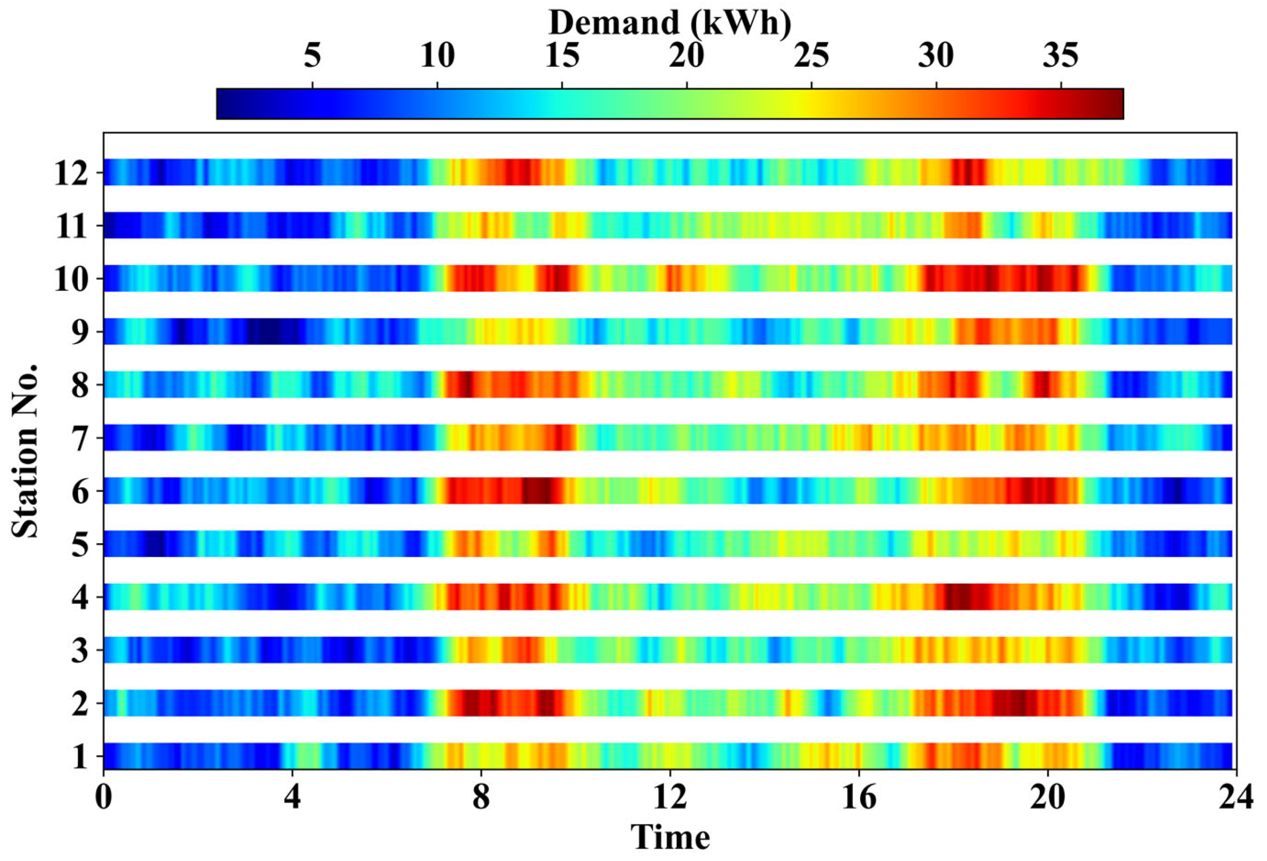
The heatmap illustrates the EV charging demand (in kWh) across 12 charging stations over a 24 h period, as shown in Figure 4. The color gradient from blue (low demand) to red (high demand) reveals significant temporal and spatial variation. Peak demand generally occurs during morning (6–9 AM) and evening (5–9 PM) hours, aligning with typical commuting patterns. Stations 10 experienced more intense demand peaks compared to others.

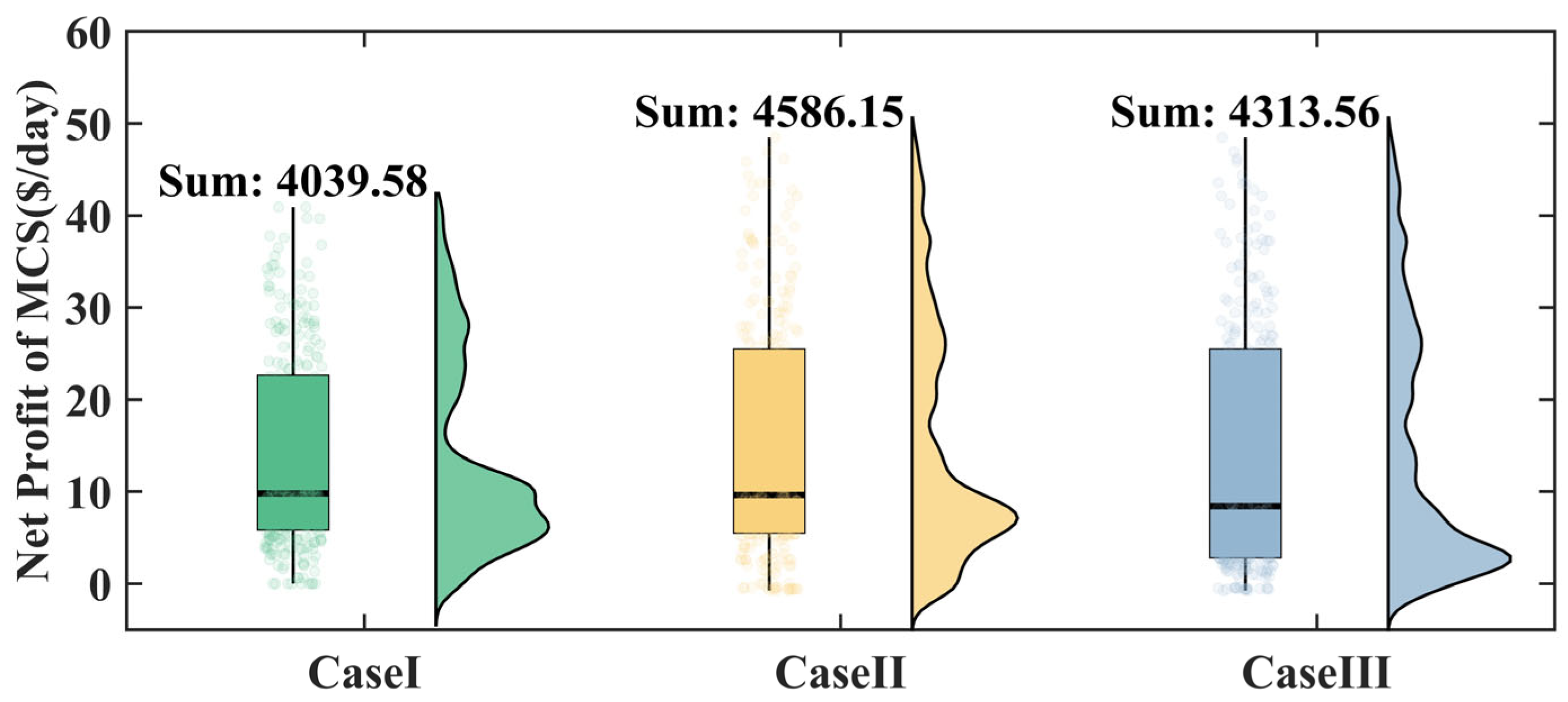
Figure 6 illustrates the distribution of daily net returns for the MCS under three distinct cases. Compared to Cases 2 and 3, Case 1 exhibits a bimodal distribution with peaks around $10, while showing fewer high-return points above approximately $38. This indicates that in Case 1, the earnings of the MCS per five-minute interval are predominantly concentrated near $10, highlighting significant revenue loss and comparatively lower profitability. In contrast, Cases 2 and 3 demonstrate broader return distributions, mainly ranging from $10 to $30, with several high-yield data points present. The upper-level model in the bi-level optimization framework identifies the station with the highest net profit every five minutes. If the estimated profit at the new location exceeds that of the current site, the MCS is relocated to provide charging services to EV users. Although Cases 2 and 3 share similar distribution patterns, Case 2 solely focuses on maximizing the MCS’s net profit, resulting in a slightly higher median profit compared to Case 3 and consequently yielding greater overall profitability.

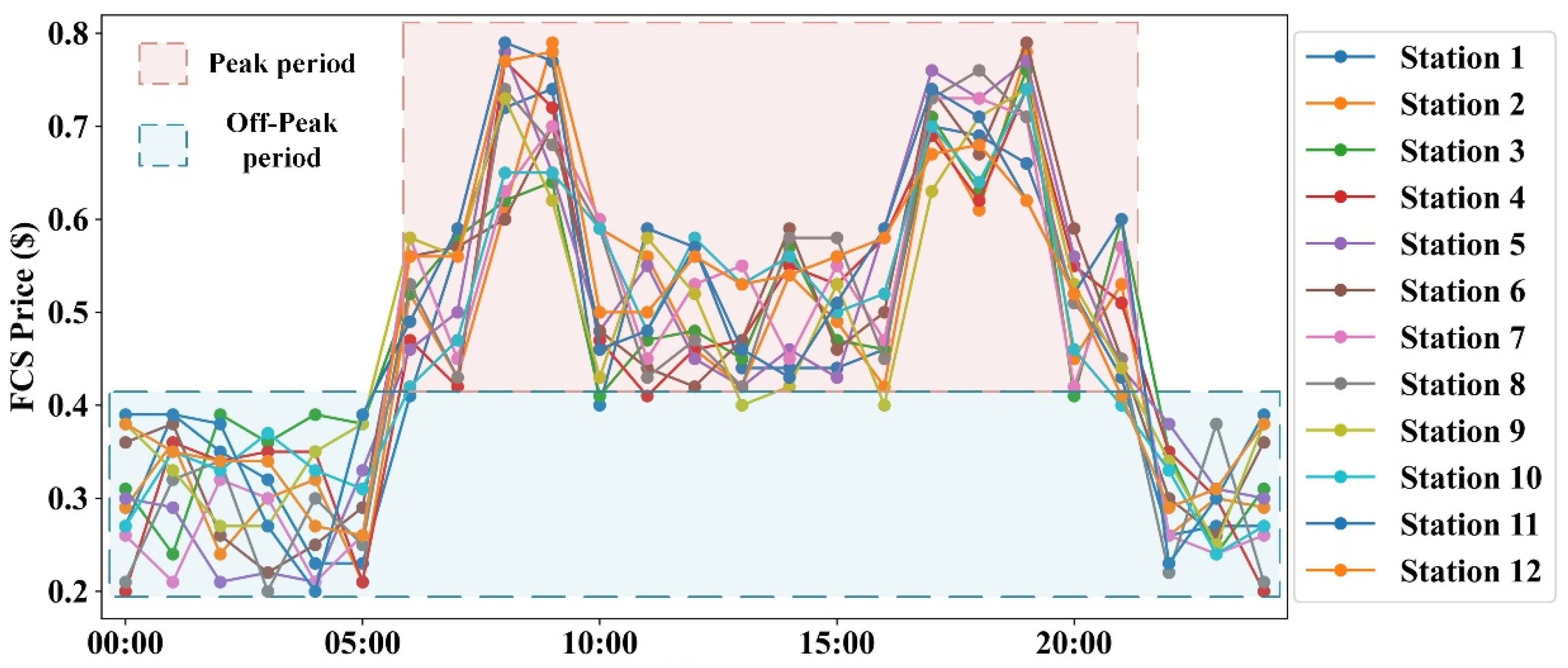
In Figure 5, the price dynamics of electric vehicle FCSs across 12 locations are depicted throughout the day. The prices peak at approximately $0.7 to $0.8 at 10:00 and 20:00, while off-peak prices typically range between $0.2 and $0.5, exhibiting lower volatility.

Table 2. Dynamic location optimization data of MCSs in case 3.

Position	Net Profit ($)	Arrival Time (hh:mm)	Departure Time (hh:mm)
Station 10	389.38	00:00	03:55
Station 1	49.07	04:05	04:40
Station 8	2050.74	04:50	10:20
Station 6	456.89	10:40	11:45
Station 10	471.65	11:50	13:00
Station 11	283.19	13:00	14:10
Station 4	87.42	14:15	14:35
Station 1	462.22	14:45	16:15
Station 3	90.81	16:20	16:55
Station 10	277.97	17:05	17:45
Station 8	767.59	17:50	18:55
Station 9	653.36	18:55	20:00
Station 10	323.22	20:00	21:00
Station 12	149.66	21:05	21:55
Station 7	116.74	22:05	23:20
Station 8	52.83	23:30	/

presents the 24 h net profit, departure time, and arrival time of the MCS at different locations in case 3. The time periods represent the scheduling arrangements for the MCS to depart from one station and arrive at the next, demonstrating the resource dispatch strategy between stations to maximize overall economic benefits.

Although Case 3 does not generate the highest standalone MCS profit in Figure 6, this does not contradict the objective of the proposed coordinated strategy. Case 2 optimizes the MCS profit independently, while Case 3 optimizes the combined profit of MCSs and FCSs from the investor’s portfolio perspective. Therefore, a lower MCS-side profit in Case 3 can be acceptable if it reduces the revenue loss of FCSs and improves the total portfolio-level profit.

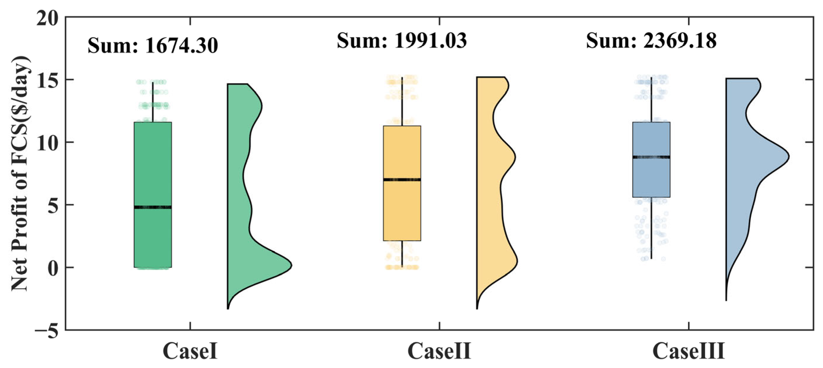
Compared to the MCSs, the differences in net profit for the FCSs under Case 3 are more pronounced when compared to the other two cases, as illustrated in Figure 7. A higher frequency of negative returns is observed in Cases 1 and 2 relative to Case 3, reflecting elevated downside risk in these configurations. This outcome can be attributed to the FCS price exceeding MCSs’ marginal cost in Cases 1 and 2, which leads the MCS to lower its price to gain more market share. However, this pricing strategy reduces demand for FCSs, subsequently lowering its revenue. Since the fixed costs remain unchanged, the profit decreases accordingly.

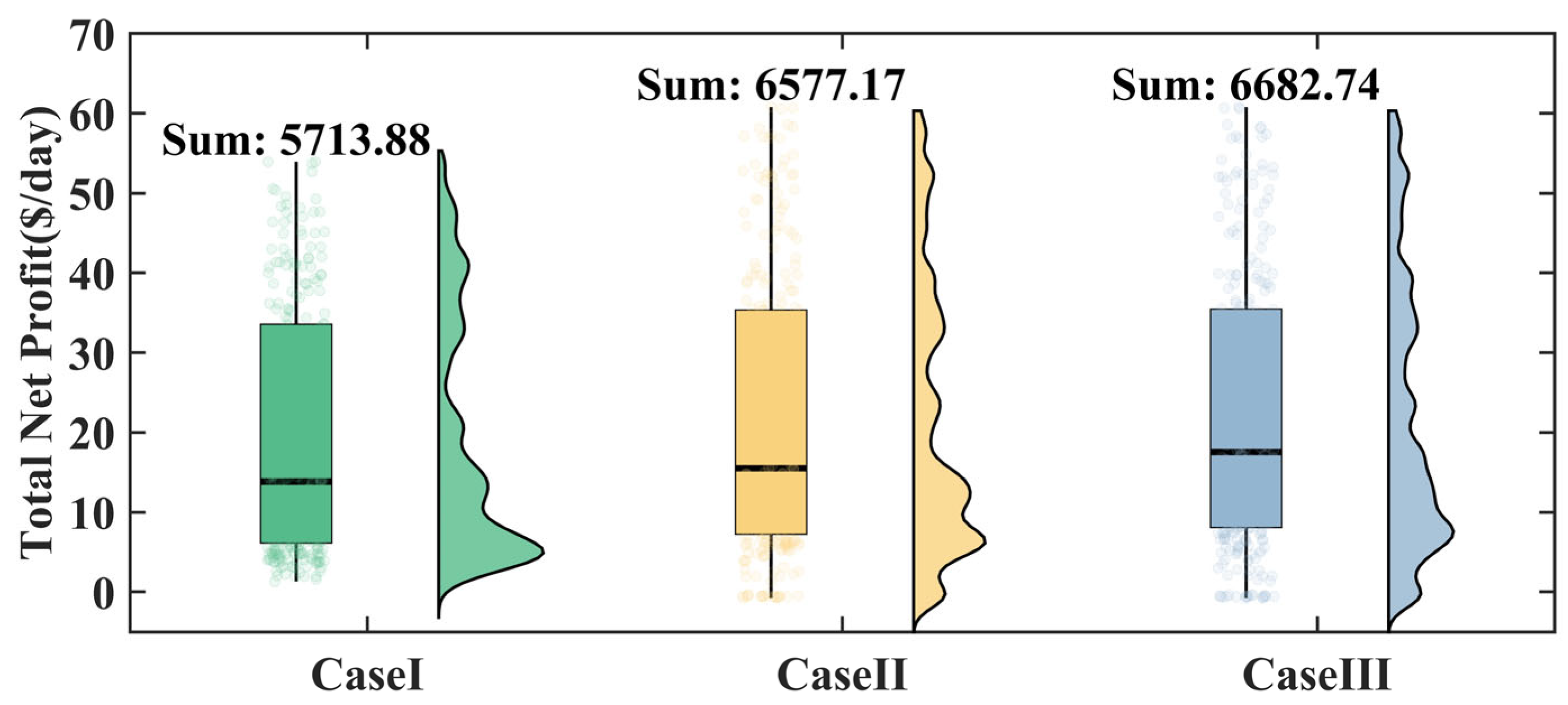
From an investor’s perspective, combining the net profits of both the MCSs and FCSs provides more practical insights. Figure 8 shows the total net profits under the three different cases ($/day). By comparison, Case 3 demonstrates the highest overall profit distribution (16.96% and 1.61% increasing of Case 1 and Case 2), while Case 1, which does not utilize the bi-level optimization of the MCS locations, consistently performs poorly. Although Case 3 performs slightly worse than Case 2 in Figure 6, it achieves the highest total net profit when combined with the FCS. A comprehensive analysis indicates that implementing the bi-level optimization model significantly improves overall profitability. Furthermore, jointly optimizing MCSs and FCSs leads to improved economic outcomes for investors, relative to optimizing MCSs alone.

Compared with Case 2, however, the increase in total net profit is only 1.61%. This result is consistent with the profit distributions shown in Figure 6 and Figure 7. Case 2 optimizes the MCS as an independent profit-seeking unit, which allows the MCS to set more competitive prices and obtain a higher standalone MCS profit. In contrast, Case 3 optimizes the combined profit of MCSs and FCSs. As a result, the MCS profit in Case 3 can be lower than that in Case 2, while the FCS-side loss is reduced and the total investor-level profit becomes slightly higher. The value of the coordinated strategy, therefore, lies mainly in mitigating internal competition between MCSs and FCSs and improving the overall portfolio outcome, rather than in increasing MCS profit alone.

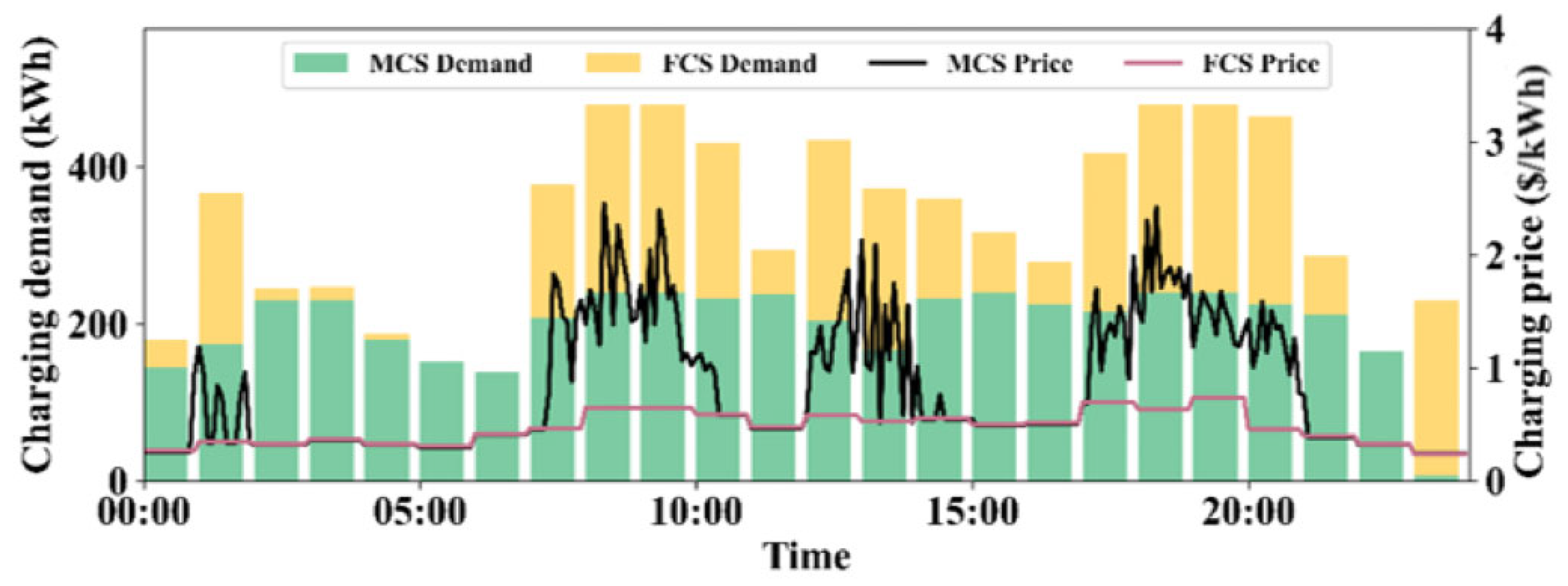
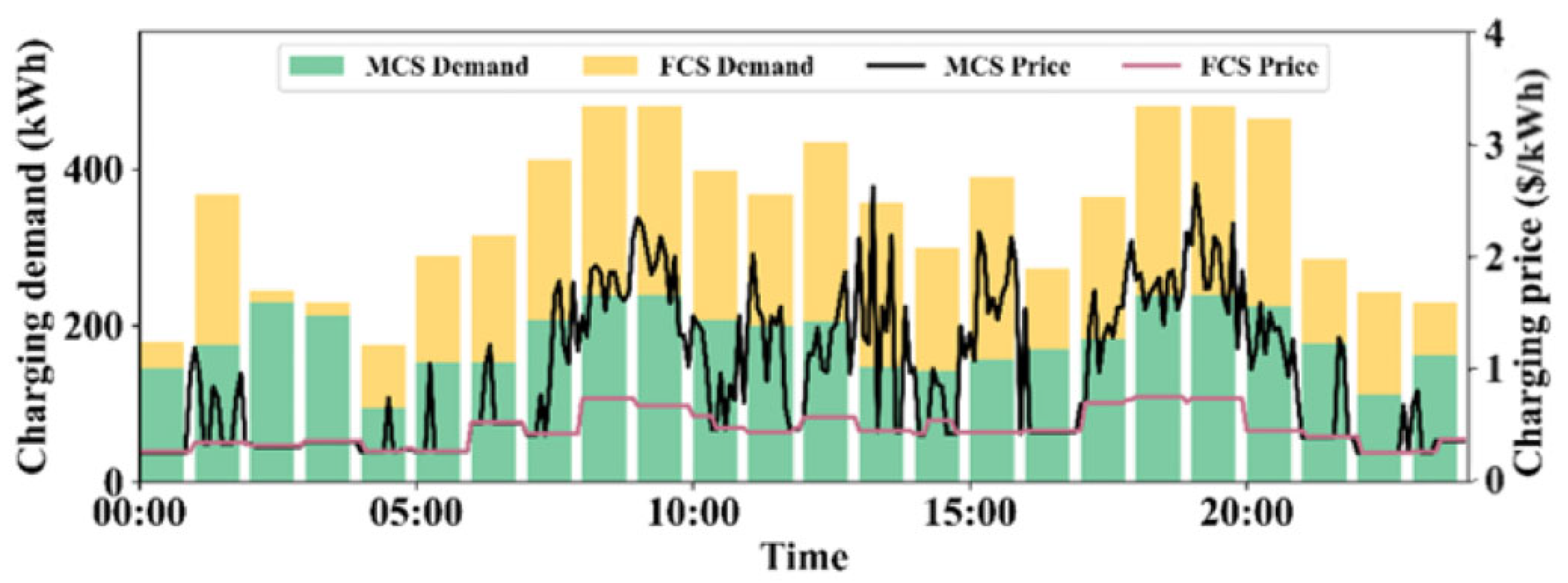
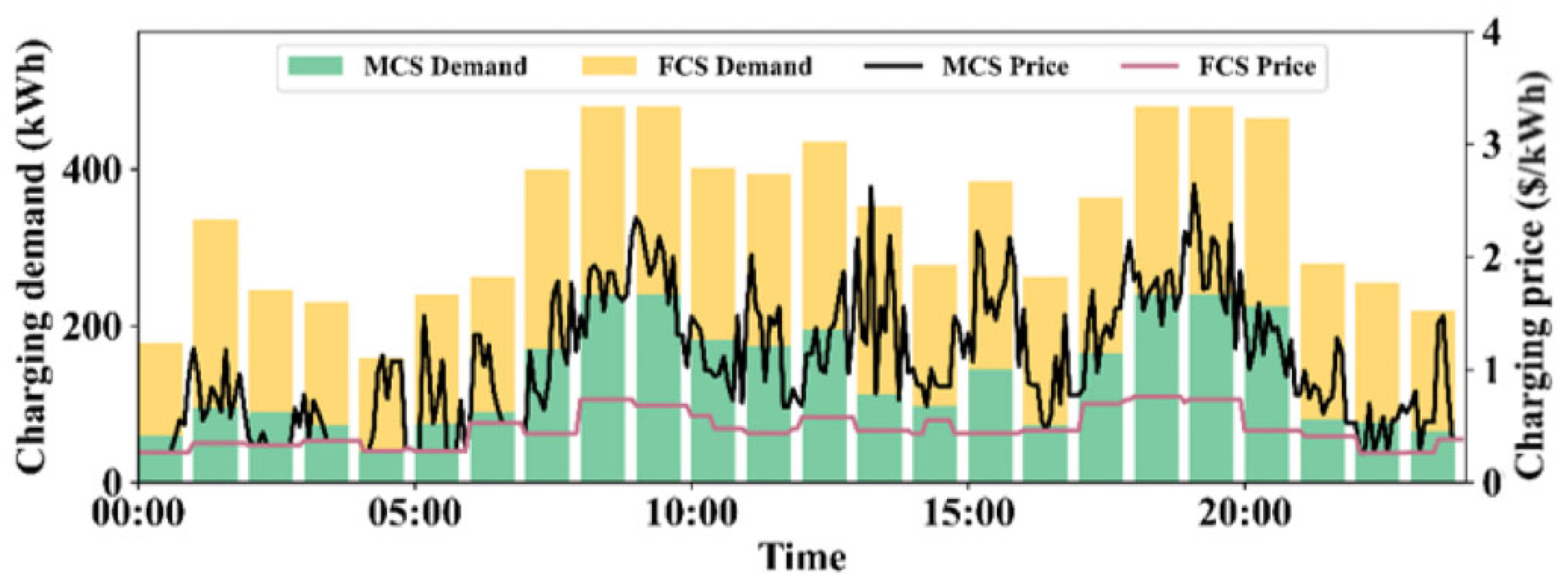
Figure 9, Figure 10 and Figure 11 illustrate the dynamic variations in charging demand and pricing for the MCSs and FCSs under the three cases over a 24 h period. In Case 1, Station 10 is the most visited station by EVs, indicating it has the highest overall demand; however, this does not necessarily imply that the station consistently experiences the highest demand at every time interval. Comparing Figure 10 and Figure 11, during off-peak electricity pricing periods—particularly from 05:00 to 06:00 and from 21:00 to 22:00—the total demand in Case 2 is higher than in Case 1. Furthermore, despite relatively stable overall MCS demand, the price fluctuations in Case 2 are notably more pronounced, leading to higher MCS prices compared to the other cases.

Additionally, by comparing Cases 2 and 3, it can be observed that the price fluctuations of the MCS became even more pronounced in Case 3. Although this may be associated with a lower MCS demand in Case 3, the net profit of the MCS is simultaneously determined by both its pricing strategy and demand; high demand does not necessarily imply higher overall profitability. By carefully examining periods with less apparent MCS pricing variations, it is evident that the MCS pricing in Cases 1 and 2 is set below that of the FCS. This pricing strategy occurs because the objective function in these cases exclusively optimizes for maximum MCS profit. Specifically, during off-peak charging periods, the MCS in Case 2 strategically sets lower prices as an incentive to attract EV users from the FCS, thus increasing MCS profits. However, from the perspective of investors considering both FCSs and MCSs jointly, the MCS and FCS are not competitors. Therefore, setting MCS prices lower than those of the FCSs to attract additional demand can negatively impact overall profitability. Conversely, during peak charging periods, when waiting times at the FCSs are longer, the MCSs in both Cases 2 and 3 set nearly identical prices to attract EV users waiting in FCS queues.

7.3. Sensitivity Analysis

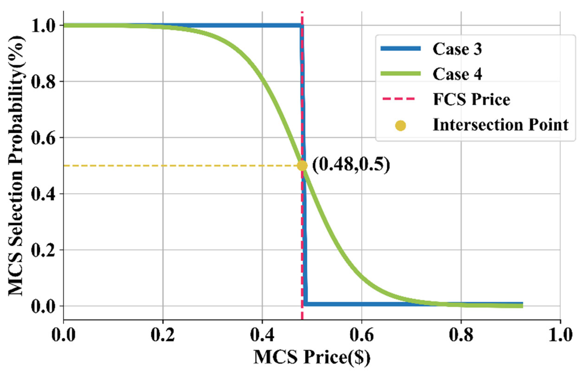
In Cases 1–3, customer decisions were determined by minimizing their charging costs through the lower-level optimization model. In this process, EV users compare the expected cost of choosing MCSs and FCSs under different charging prices, travel conditions, and queuing states. Therefore, the obtained charging demand is not assigned by a fixed probability but is endogenously generated from the cost-minimization behavior of customers. Since this behavioral response plays an important role in the interaction between charging demand and operator pricing, a further sensitivity analysis was conducted to examine how customers react to variations in MCS pricing. This analysis also provides a direct comparison between the conventional probabilistic customer choice model and the model proposed in this paper. In the sensitivity test, the FCS charging price was fixed at 0.48, while the MCS charging price was gradually varied over the selected price range. This setting highlights whether the customer-choice model can capture the switching behavior of EV users when the relative price advantage of MCS changes.

Figure 12 presents this sensitivity analysis, showing how variations in MCS prices affect the proportion of customers choosing MCSs. From Figure 12, when the FCS price is fixed at 0.48, the conventional model (Case 4) exhibits a relatively smooth and gradual decline in the probability of selecting MCSs as the MCS price increases from 0.2 to 0.7. In contrast, the proposed model displays a sharp decline in MCS selection probability, dropping rapidly to zero as the MCS price approaches 0.48. Analyzing this behavior from a practical perspective, under the assumption that all other parameters remain constant, and the queuing model applies, EV users prefer charging at MCSs when its price is lower. However, as the MCS price increases and eventually exceeds the FCS price, users rapidly shift their preference toward FCSs. This observed behavior contradicts the conventional probabilistic choice model but aligns closely with realistic user behavior. Thus, the improved selection model (lower-level optimization) proposed in this paper better captures realistic customer decisions, leading to results that are more consistent with actual market conditions.

8. Conclusions

This study proposes a bi-level optimization model that integrates customer-side charging decisions with the overall net profit maximization of both MCSs and FCSs to determine the dynamic location deployment and residence time of MCSs. In the lower level, customer behavior across different locations and time periods is pre-optimized to derive charging decisions. The upper level utilizes EV users’ charging decisions from the lower level to maximize total net profit, thereby determining the optimal MCS locations and docking durations. Compared with the fixed-location benchmark, the proposed MDL-C model achieves a substantial improvement in total net profit by allowing the MCS to respond to spatiotemporal variations in charging demand. In the tested scenario, the total net profit increases by 16.96% relative to fixed siting. Compared with the MCS-only optimization benchmark, the total net profit increases by 1.61%, but it balances the profit allocation between MCSs and FCSs and reduces internal competition within the investor’s charging-service portfolio. Simulation results further validate the universality and superiority of the lower-level optimization model over conventional stochastic utility theory. Additionally, the dynamic location planning of MCSs enables rapid responses to localized charging demand fluctuations, alleviating power supply pressures caused by insufficient charger availability in FCSs.

References

1. Cao, Y.; Cui, J.; Liu, S.; Li, X.; Zhou, Q.; Hu, C.; Zhuang, Y.; Liu, Z. A Holistic Review on E-Mobility Service Optimization: Challenges, Recent Progress, and Future Directions. IEEE Trans. Transp. Electrif. 2024, 10, 3712–3741. [Google Scholar] [CrossRef]
2. Ray, S.; Kasturi, K.; Patnaik, S.; Nayak, M.R. Review of electric vehicles integration impacts in distribution networks: Placement, charging/discharging strategies, objectives and optimisation models. J. Energy Storage 2023, 72, 108672. [Google Scholar] [CrossRef]
3. Lin, J.; Qiu, J.; Tao, Y.; Sun, X. Planning of Electric Vehicle Charging Stations with PV and Energy Storage Using a Fuzzy Inference System. IEEE Trans. Transp. Electrif. 2024, 10, 5894–5909. [Google Scholar] [CrossRef]
4. Global EV Outlook 2024 IEA, 2024. Available online: https://www.iea.org/reports/global-ev-outlook-2024 (accessed on 16 March 2025).
5. Khatua, A.; Kumar, R.R.; De, S.K. Institutional enablers of electric vehicle market: Evidence from 30 countries. Transp. Res. Part A Policy Pract. 2023, 170, 103612. [Google Scholar] [CrossRef]
6. Afshar, S.; Macedo, P.; Mohamed, F.; Disfani, V. A Literature Review on Mobile Charging Station Technology for Electric Vehicles. In Proceedings of the 2020 IEEE Transportation Electrification Conference & Expo (ITEC), Chicago, IL, USA; IEEE: Piscataway, NJ, USA, 2020; pp. 1184–1190. [Google Scholar]
7. He, K.; Jia, H.; Mu, Y.; Yu, X.; Zhou, Y.; Wu, J.; Dong, X. Leasing Business Model for Truck Mobile Charging Stations: From the View of Operators. IEEE Trans. Transp. Electrif. 2025, 11, 8811–8823. [Google Scholar] [CrossRef]
8. Liang, Z.; Chung, C.; Yin, X.; Wang, Q.; Chen, H.; Zhu, J. Scheduling for Hybrid Microgrids with Renewable Energy Sources and Hydrogen Storage: Data-Correlated Uncertainty Modeling and Semi-Convex Relaxation. IEEE Trans. Sustain. Energy 2026, 1–17. [Google Scholar] [CrossRef]
9. Afshar, S.; Macedo, P.; Mohamed, F.; Disfani, V. Mobile charging stations for electric vehicles—A review. Renew. Sustain. Energy Rev. 2021, 152, 111654. [Google Scholar] [CrossRef]
10. Gupta, R.S.; Tyagi, A.; Anand, S. Optimal allocation of electric vehicles charging infrastructure, policies and future trends. J. Energy Storage 2021, 43, 103291. [Google Scholar] [CrossRef]
11. Yao, L.; Damiran, Z.; Lim, W.H. Optimal Charging and Discharging Scheduling for Electric Vehicles in a Parking Station with Photovoltaic System and Energy Storage System. Energies 2017, 10, 550. [Google Scholar] [CrossRef]
12. Tamai, G. What Are the Hurdles to Full Vehicle Electrification? [Technology Leaders]. IEEE Electrif. Mag. 2019, 7, 5–11. [Google Scholar] [CrossRef]
13. Beyazıt, M.A.; Taşcıkaraoğlu, A. Electric vehicle charging through mobile charging station deployment in coupled distribution and transportation networks. Sustain. Energy Grids Netw. 2023, 35, 101102. [Google Scholar] [CrossRef]
14. Qureshi, U.; Ghosh, A.; Panigrahi, B.K. Scheduling and routing of mobile charging stations with stochastic travel times to service heterogeneous spatiotemporal electric vehicle charging requests with time windows. IEEE Trans. Ind. Appl. 2022, 58, 6546–6556. [Google Scholar] [CrossRef]
15. Ding, Y.; Qu, G.; Chen, X.; Wang, J.; Song, J.; He, G. Deep Reinforcement Learning-Based Spatiotemporal Decision of Utility-Scale Highway Portable Energy Storage Systems. IEEE Trans. Ind. Appl. 2024, 60, 966–975. [Google Scholar] [CrossRef]
16. Zhang, Y.; Liu, X.; Wei, W.; Peng, T.; Hong, G.; Meng, C. Mobile charging: A novel charging system for electric vehicles in urban areas. Appl. Energy 2020, 278, 115648. [Google Scholar] [CrossRef]
17. Liu, L.; Zhang, H.; Xu, J.; Wang, P. Providing Active Charging Services: An Assignment Strategy with Profit-Maximizing Heat Maps for Idle Mobile Charging Stations. IEEE Trans. Mob. Comput. 2024, 23, 2139–2152. [Google Scholar]
18. Liu, L.; Liu, S.; Wu, J.; Xu, J. A Placement Strategy for Idle Mobile Charging Stations in IoEV: From the View of Charging Demand Force. IEEE Trans. Intell. Transp. Syst. 2024, 25, 3870–3884. [Google Scholar] [CrossRef]
19. He, K.; Jia, H.; Mu, Y.; Yu, X.; Dong, X.; Deng, Y. Coordinated Planning of Fixed and Mobile Charging Facilities for Electric Vehicles on Highways. IEEE Trans. Intell. Transp. Syst. 2023, 24, 10087–10098. [Google Scholar] [CrossRef]
20. Cui, J.; Jiang, W.; Wu, C. Pricing mechanism design for future EV charging station with hybrid fixed and mobile charging modes. Appl. Energy 2024, 380, 125033. [Google Scholar] [CrossRef]
21. Shangguan, Z.; Yang, B.; Gao, F.; Tu, J.; Tang, Y. A crowdsourcing renewable energy delivery framework with dynamic pricing and routing policy. IFAC-PapersOnLine 2022, 55, 54–59. [Google Scholar] [CrossRef]
22. Ahmed, H.M.A.; Sindi, H.F.; Azzouz, M.A.; Awad, A.S.A. Optimal Sizing and Scheduling of Mobile Energy Storage Toward High Penetration Levels of Renewable Energy and Fast Charging Stations. IEEE Trans. Energy Convers. 2022, 37, 1075–1086. [Google Scholar] [CrossRef]
23. Liang, Z.; Yin, X.; Chung, C.Y.; Rayeem, S.K.; Chen, X.; Yang, H. Managing Massive RES Integration in Hybrid Microgrids: A Data-Driven Quad-Level Approach with Adjustable Conservativeness. IEEE Trans. Ind. Inform. 2025, 21, 7698–7709. [Google Scholar] [CrossRef]
24. Wang, C.; Lin, X.; He, F.; Shen, M.Z.-J.; Li, M. Hybrid of fixed and mobile charging systems for electric vehicles: System design and analysis. Transp. Res. Part C Emerg. Technol. 2021, 126, 103068. [Google Scholar] [CrossRef]
25. Lai, S.; Qiu, J.; Tao, Y.; Zhao, J. Pricing Strategy for Energy Supplement Services of Hybrid Electric Vehicles Considering Bounded-Rationality and Energy Substitution Effect. IEEE Trans. Smart Grid 2023, 14, 2973–2985. [Google Scholar] [CrossRef]
26. Liu, L.; Xi, Z.; Zhu, K.; Wang, R.; Hossain, E. Mobile Charging Station Placements in Internet of Electric Vehicles: A Federated Learning Approach. IEEE Trans. Intell. Transp. Syst. 2022, 23, 24561–24577. [Google Scholar] [CrossRef]
27. Tu, W.; Li, Q.; Fang, Z.; Shaw, S.-L.; Zhou, B.; Chang, X. Optimizing the locations of electric taxi charging stations: A spatial–temporal demand coverage approach. Transp. Res. Part C Emerg. Technol. 2016, 65, 172–189. [Google Scholar] [CrossRef]
28. Zamparini, L.; Reggiani, A. Meta-analysis and the value of travel time savings: A transatlantic perspective in passenger transport. Netw. Spat. Econ. 2007, 7, 377–396. [Google Scholar] [CrossRef]
29. Allen, A.O. Probability, Statistics, and Queuing Theor; Academic Press: New York, NY, USA, 2014. [Google Scholar]
30. Yang, J.; He, F.; Shen, Z.-J.M.; Lin, X. Dynamic Pricing and Service Fulfillment of Mobile Charging Systems with Stochastic Demands. Prod. Oper. Manag. 2025, 34, 2032–2049. [Google Scholar] [CrossRef]
31. Jiang, M.; Morikawa, T. Theoretical analysis on the variation of value of travel time savings. Transp. Res. Part A Policy Pract. 2004, 38, 551–571. [Google Scholar] [CrossRef]
32. Dong, X.H.; Mu, Y.F.; Jia, H.J.; Wu, J.Z.; Yu, X. Planning of fast EV charging stations on a round freeway. IEEE Trans. Sustain. Energy 2016, 7, 1452–1461. [Google Scholar] [CrossRef]
33. Schneider, K.P.; Mather, B.A.; Pal, B.C.; Ten, C.-W.; Shirek, G.J.; Zhu, H.; Fuller, J.C.; Pereira, J.L.R.; Ochoa, L.F.; de Araujo, L.R.; et al. Analytic Considerations and Design Basis for the IEEE Distribution Test Feeders. IEEE Trans. Power Syst. 2018, 33, 3181–3188. [Google Scholar] [CrossRef]
Figure 1. Optimal dynamic pricing and deployment framework for MCSs and FCSs.
Electronics 15 03032 g001
Figure 2. The collaborative operation state of MCSs and FCSs.
Electronics 15 03032 g002
Figure 3. Coupled IEEE 33-bus distribution system and urban road network with 14 candidate coupling nodes and 47 road links.
Electronics 15 03032 g003
Figure 4. EV charging load distribution at each station over 24 h.
Electronics 15 03032 g004
Figure 5. FCS charging price of EV at each station in 24 h.
Electronics 15 03032 g005
Figure 6. The distribution of MCSs’ net profit for each case.
Electronics 15 03032 g006
Figure 7. The distribution of FCSs’ net profit for each case.
Electronics 15 03032 g007
Figure 8. The distribution of the total net profit for each case.
Electronics 15 03032 g008
Figure 9. Charging demand and price of Case 1.
Electronics 15 03032 g009
Figure 10. Charging demand and price of Case 2.
Electronics 15 03032 g010
Figure 11. Charging demand and price of Case 3.
Electronics 15 03032 g011
Figure 12. The impact of charging price on MCS selection probability.
Electronics 15 03032 g012