Article

Stability- and Safety-Constraint Reinforcement Learning for Pedestrian Avoidance in Occluded Urban Driving

Department of Computer and Network Engineering, The University of Electro-Communications, 1-5-1 Chofugaoka, Chofu 182-8585, Tokyo, Japan
*
Author to whom correspondence should be addressed.
Electronics 2026, 15(14), 3026; https://doi.org/10.3390/electronics15143026
Submission received: 4 June 2026 / Revised: 2 July 2026 / Accepted: 6 July 2026 / Published: 9 July 2026
(This article belongs to the Section Artificial Intelligence)

Abstract

Road traffic accidents continue to be a major global cause of fatalities, disproportionately affecting pedestrians and other vulnerable road users. While deep reinforcement learning has proven effective in handling complex navigation tasks, providing formal stability and safety guarantees during both training and deployment remains a significant challenge. This paper introduces a dual-layer safety-aware framework for pedestrian avoidance in occluded urban driving. During training, a first-order Control Lyapunov–Barrier Function is integrated with Proximal Policy Optimization to promote goal-reaching stability and obstacle avoidance: the analytic Lie derivatives of the Lyapunov and barrier functions are embedded as a modifier in the advantage estimate, providing explicit stability and safety signals that accelerate convergence toward safe, goal-reaching behavior without disrupting the standard policy update. At deployment, a higher-order Control Lyapunov–Barrier Function, realized through a quadratic programming safety filter, acts as a safety shield that projects the nominal acceleration onto the intersection of the second-order Lyapunov and barrier feasibility sets; the barrier function is further extended with relative velocity terms to account for dynamic pedestrian motion. Experiments with a four-wheeled vehicle in the Webots simulator show that the framework reliably reaches the goal, avoids an occluded pedestrian across a range of crossing speeds, and improves task success rates and safety-constraint adherence relative to Proximal Policy Optimization and a conventional higher-order safety filter baseline, particularly during emergency braking maneuvers.

1. Introduction

Road accidents have emerged as a critical global crisis in recent years, culminating in alarmingly high mortality rates. The 2019 statistics published by the World Health Organization reveal that approximately 1.19 million road users tragically lost their lives, predominantly in the 5 to 29 age group, which accounts for a staggering 30 percent of total fatalities. The data also highlights the distribution of fatalities among various road user categories. Two-wheeled and three-wheeled vehicles lead the fatality rates at 30 percent, followed closely by four-wheeled vehicles at 25 percent, and pedestrians, who represent around 20 percent of casualties [1]. Furthermore, data from the U.S. National Highway Traffic Safety Administration shows that vehicle accidents in 2019 inflicted approximately $340 billion in damage [2]. In light of distressing figures, it is imperative to recognize that road safety is a pressing issue that demands the implementation of effective safety measures. Alongside this, innovative advancements in road safety technology are being developed to create better conditions for both drivers and pedestrians.
The surge in autonomous driving technology has captured the attention of researchers and the public alike [3]. Breakthroughs in safety technologies, particularly the incorporation of Artificial Intelligence (AI), have led to the development of advanced algorithms for autonomous vehicles, marking significant progress toward fully self-driving systems grounded in empirical data from complex driving environments [4]. Central to these strides are Advanced Driver Assistance Systems (ADAS), which play a vital role in enhancing safety through features such as Automatic Emergency Braking (AEB), Lane Keeping Assistance (LKA), and Blind Spot Warning (BSW). However, significant hurdles, including unintended emergency braking in the absence of obstacles and unreliable system performance, remain, underscoring the urgent need for refinement in ADAS safety measures to ensure greater protection for all road users [5].
Deep reinforcement learning (DRL) has emerged as a fundamental aspect of machine decision-making [6], grounded in the principles of Markov Decision Processes (MDP). This approach employs trial-and-error to enhance the effectiveness of agents across varied environments. In the realm of autonomous driving, DRL empowers modern vehicles to enhance their collision-avoidance strategies by analyzing real-time data from onboard sensors. This method demonstrates the system’s capacity for immediate responsiveness while actively informing the vehicle’s decision-making process. The adaptability and robustness of DRL make it ideally suited for both simulation [7,8,9] and practical applications [10,11], solidifying its position as an advanced solution for safer navigation in complex driving scenarios [12].
Control Lyapunov–Barrier Function (CLBF), in conjunction with quadratic programming (QP), represents a groundbreaking algorithm approach to nonlinear control that ensures stability by guiding systems toward desired states while simultaneously maintaining safety through hazard avoidance [13,14]. In the context of autonomous driving, these algorithms tackle intricate scenarios [15,16]. Additionally, autonomous vehicles leverage CLBF constraints to navigate unfamiliar environments safely, integrating sensory data for obstacle detection and optimizing via QP, thereby surpassing conventional control techniques [17]. Importantly, CLBF adheres to constraints that verify real-time safety [18], providing essential validation of the stability and safety requirements in autonomous driving [19].
In terms of cutting-edge controller algorithms, with the advancement of DRL, the combination of CLBF with DRL has become increasingly important for learning under stability and safety constraints in challenging circumstances. The CLBF algorithm leverages the safety constraints proof, introducing a modification to CLBF to enable the agent to learn about the policy’s stability and safety objective, allowing safe exploration in model-based reinforcement learning for collision avoidance in uncertain scenarios [20,21]. Beyond the QP-based filtering adopted in this work, backstepping-based formulations offer a complementary route to enforcing safety during learning: a Barrier Lyapunov Function can be embedded directly into an optimized-backstepping actor–critic controller to constrain the state variables to a designed safety region throughout training under unknown system uncertainty [22], while control barrier performance formulations reconcile safety and performance constraints with actuation limits in cooperative multi-vehicle settings through parallel dynamic event-triggering that reduces the controller update frequency [23]. Likewise, the Control Barrier Function is generalized with adaptive coefficient mechanisms via model-based reinforcement learning to enhance the likelihood of safe policy optimization, achieving significantly faster convergence and reducing constraint violations compared with baseline methods [24]. In a hierarchical control context, it is separated into a high-level controller that creates high-level navigation commands (e.g., forward, backward, left, and right) and a low-level controller that controls the trajectory to achieve the objective. With the combination of a deep reinforcement learning-based high-level controller and a CLBF-QP controller as a low-level controller on a stability and safety controller for collision avoidance, the controllers perform computational efficiency and robustness in scenarios involving sophisticated circumstances, e.g., lane-changing maneuvers and reaching goals safely, as well as accidental avoidance, both static and dynamic [25,26].
In this study, we integrate deep reinforcement learning with Control Lyapunov–Barrier Functions to enhance pedestrian avoidance in obstructed driving scenarios. Our key contributions are as follows:
  • A co-designed Lyapunov–barrier spanning training and deployment. We train a first-order CLBF-modified PPO policy for slip-angle control and enforce a higher-order CLBF-QP filter on acceleration during deployment. Both stages are built on identical Lyapunov and barrier definitions. Unlike hierarchical learning controllers that independently design a safety filter beneath a separately trained decision policy, this shared-certificate design aligns the learned policy’s inductive bias with the geometry enforced by the filter and the runtime context.
  • A critic-independent stability and safety signal for the policy optimization. By computing this signal in closed form rather than bootstrapping it from the critic, we inject explicit stability and safety information that accelerates convergence toward collision-free, goal-reaching behavior without altering the standard PPO update. This differs from constrained policy optimization approaches to safe RL, where the barrier constraint is enforced through a learned cost–value estimate or a Lagrangian multiplier that must itself be estimated during training [20,21,24]; our signal is available in closed form from the first control step, requiring no additional value function, dual variable, or warm-up period before it becomes informative.
  • A relative velocity higher-order barrier for dynamic pedestrian avoidance. We extend the higher-order barrier to include a closing-rate term, allowing the safety constraint at deployment time to respond to the relative velocity between the vehicle and a moving pedestrian, rather than relying on relative position alone. This generalizes the runtime filter from static to actively crossing obstacles.
To highlight the specific novelty of our approach, Table 1 compares the proposed framework with the most closely related methods in control-based, hierarchical learning-based, and safe reinforcement learning across five key dimensions.
As shown in Table 1, previous CLBF-QP controllers ensure safety without incorporating any learned components. In contrast, hierarchical methods only learn a discrete high-level decision and operate an independently designed QP filter underneath. Safe reinforcement learning techniques, on the other hand, integrate a barrier constraint during training but do not provide a filter for deployment. The proposed framework stands out as the only one that (i) learns a continuous control policy, where the policy’s advantage is influenced by the same Lyapunov and barrier certificates enforced by the runtime HOCLBF–QP filter, and (ii) incorporates a relative velocity term for actively crossing pedestrians, which has been validated at a real-time control rate in a high-fidelity simulator.
This paper is organized as follows: Section 2 describes the methodologies used, including the bicycle vehicle dynamic model, control-affine equations, and the design principles for the Control Lyapunov Function (CLF) and Control Barrier Function (CBF) for both first-order and second-order systems. It also introduces the modified advantage estimates using Proximal Policy Optimization (PPO) and the Optimal Control with Lyapunov–Barrier Function and Quadratic Programming (HOCLBF-QP) framework. Section 3 outlines the simulation environment, vehicle platform and sensing, and the Deepbots framework. Section 4 presents the simulation results, comparing the proposed approach with baseline methods (PPO with MLP and PPO-LSTM) and examining how different weights affect the agent’s training and driving trajectory. We also analyze the effect of the class- K function on HOCLBF-QP in terms of acceleration and braking behavior, compare the integration of CLBF-PPO-HOCLBF-QP with traditional HOCLBF-QP across a range of pedestrian crossing speeds, and finally report the per-step computational time of the controller to assess its real-time feasibility. Section 5 addresses research limitations, and Section 6 concludes the paper with suggestions for future research directions.

2. Methodology

In a comprehensive autonomous driving algorithm that emphasizes the maneuverability of self-driving vehicles, Figure 1 provides an overview of the proposed framework. This section will introduce each component in the order they appear in the figure.
Section 2.1 develops the vehicle model by simplifying the four-wheeled vehicle into a kinematic bicycle model, which is presented in control-affine form through Equations (1)–(5). This model serves as the foundation for all subsequent Lyapunov and barrier constraints, represented by the Environment block in Section 2.1.
Section 2.2 introduces the certificate functions. Section 2.2.1 defines the first-order Control Lyapunov and Control Barrier Functions used for slip-angle control during training. Section 2.2.2 extends these functions to include higher-order functions used for acceleration control during deployment.
Section 2.3 discusses the Proximal Policy Optimization algorithm along with the CLBF-modified advantage estimate presented in (30). This estimate incorporates the first-order Lie derivatives into the policy gradient and corresponds to the PPO block in Figure 1. The design of the associated rewards and penalties is detailed in Section Rewards and Penalty Calculation.
Lastly, Section 2.4 formulates the higher-order CLBF-QP safety filter expressed in (37), which controls the agent’s acceleration at runtime and corresponds to the HOCLBF-QP block in Figure 1. The policy outlined in Section 2.3 outputs the slip-angle command β π , while the filter in Section 2.4 generates the acceleration command a π . Together, these commands constitute the control input applied to the vehicle model described in Section 2.1.

2.1. Bicycle Vehicle Dynamics

In this study, we seek to streamline the dynamics of a vehicle by narrowing our focus to the kinematic aspects of the bicycle dynamic model. Our examination deliberately omits considerations of reference forces and mass properties. By concentrating on the kinematics, we aim to enhance our understanding of the vehicle’s motion in a more straightforward manner, allowing for clearer insights into its behavior and performance characteristics without the complexities introduced by additional dynamic forces and mass influences. This approach will enable us to develop more efficient models for analyzing vehicle dynamics in various applications.
This kinematic model intentionally simplifies the vehicle’s longitudinal and lateral dynamics. It excludes factors such as tire forces, mass and yaw inertia, lateral weight transfer, and the interaction between sideslip and yaw rate. The wheels are assumed to roll without slipping, maintaining a kinematic link between the heading and velocity vector through the slip angle mentioned in (1). This simplification is valid as long as the lateral forces on the tires are low. At low speeds and with gentle lateral accelerations, the tires function within their linear range, resulting in minor actual sideslip, allowing the kinematic model to closely reflect the vehicle’s true trajectory. This is supported by Polack et al. [27], who demonstrate that the kinematic bicycle model is effective for planning achievable low-speed paths. However, as speed, path curvature, or tire friction increases, sideslip becomes significant, and the vehicle’s stability is then governed by the interaction between lateral and yaw dynamics rather than kinematics alone. In this scenario, the vehicle can skid or spin—losing stability—even with an active motion controller, as discussed by Hu et al. [28], who point out that this lack of stability arises from sideslip and yaw-rate behaviors that the kinematic model fails to account for. The current study focuses on the initial scenario, limiting the agent to a maximum longitudinal speed of 1 m/s with moderate steering demands, making the no-slip kinematic model an appropriate standard for control at this speed. The limits of this simplification and the transition to a more complex dynamic model are further explored in Section 5.
Figure 2 illustrates the motion dynamics of a bicycle in a two-dimensional plane. In this model, the front and rear wheels of the bicycle are represented as single wheels located at the center of each side of the vehicle. The bicycle adjusts its course through linear acceleration a and can change direction based on different steering angles δ , which are influenced by the slip angle β .
β = arctan l f l f + l r tan ( δ )
where l f and l r are the distances between the center of mass and the front wheels and the rear wheels, respectively. The kinematic bicycle equations corresponding to this vehicle model are expressed as follows [27]:
(2a) x ˙ = v cos ( θ + β ) (2b) y ˙ = v sin ( θ + β ) (2c) θ ˙ = v l r sin ( β ) (2d) v ˙ = a
where [ x ˙ , y ˙ ] are the vehicle’s x-y axis velocity at the center of mass, v is the vehicle’s velocity, a denotes the vehicle’s linear acceleration, θ denotes the orientation angle of the vehicle. Here, l f and l r represent the distances from the center of mass to the front and rear axles, respectively.
Considering that the slip angle is small, we can make the approximations cos β 1 and sin β β . This simplification leads us to the kinematic vehicle dynamic equation for small β , which is useful for analyzing the motion of the vehicle under these conditions.
(3a) x ˙ = v cos ( θ ) v sin ( θ ) β (3b) y ˙ = v sin ( θ ) + v cos ( θ ) β (3c) θ ˙ = v l r β (3d) v ˙ = a
Regarding the motion analysis of the Control Lyapunov–Barrier Function, the control-affine equation is written as:
x ˙ = f ( x ) + g ( x ) u
where x X R n denotes a state within the set of constraints of the vehicle at a given time. The term f ( x ) represents the drift component, which describes the system’s behavior in the absence of control input, while g ( x ) is a state-dependent function that modifies the control input u. In the context of the bicycle vehicle dynamic model, the control-affine equation can be expressed in matrix form as follows:
x ˙ y ˙ θ ˙ v ˙ = v cos ( θ ) v sin ( θ ) 0 0 + 0 v sin ( θ ) 0 v cos ( θ ) 0 v l r 1 0 a β

2.2. Control Lyapunov Functions (CLFs) and Control Barrier Functions (CBFs)

Although both Control Lyapunov Functions and Control Barrier Functions are scalar certificate functions evaluated along system trajectories, they fulfill distinct yet complementary roles. A Control Lyapunov Function is designed to certify stability: it behaves as an energy-like function that remains positive when away from the goal and is constrained to decrease along the trajectory. This descent enforces the system’s approach towards the desired equilibrium. Conversely, a Control Barrier Function ensures safety by defining a safe set as its zero-superlevel set. It is constrained to maintain forward invariance, ensuring that any trajectory originating within the safe region will remain.
The introduction of both functions is crucial for tasks such as pedestrian avoidance, which require simultaneous adherence to stability and safety principles. The vehicle must not only reach its goal—addressed by the stability aspect of the Control Lyapunov Function—but also avoid entering hazardous areas around obstacles or pedestrians—managed by the Control Barrier Function. Each function alone is insufficient: a purely stabilizing controller may inadvertently navigate through obstacles, while a solely safety-focused filter may lack the motivation to reach the target, potentially halting before achieving the desired outcome. This limitation has been evidenced by the traditional HOCLBF-QP baseline, as discussed in Section 4.3.
The integration of both functions during the training process, reflected in the advantage estimate and utilized within the quadratic program at deployment, enables the formulation of control inputs that are both goal-directed and safe.

2.2.1. First-Order Control Lyapunov Function and Control Barrier Functions

The Lyapunov stability theory is commonly applied to assess the stability of dynamical systems. Specifically, a positive Lyapunov function V ( x ) is considered stable if its derivative satisfies V ˙ ( x ) 0 . Furthermore, if it holds that V ˙ ( x ) c V ( x ) for some c > 0 , the dynamical system is deemed exponentially stable or convergent [29]. The linear-quadratic optimal control based on Control Lyapunov Functions (CLFs) for nonlinear systems is motivated by optimization problems related to affine-control systems. The definition of CLF is outlined as follows [30,31]:
c 1 x 2 V ( x ) c 2 x 2
inf u U [ L f V ( x ) + L g V ( x ) u ] 0
where constants c 2 > c 1 > 0 . L f V ( x ) V ( x ) x f ( x ) and L g V ( x ) V ( x ) x g ( x ) denote the partial derivative of function V ( x ) along the control-affine equation.
In terms of safety constraints of the vehicle, Control Barrier Functions (CBFs) are functions that ensure the vehicle’s movement invariance from a given set of states C R n . A vector CBF definition allows the various barrier function constraints’ implementation in order to manipulate a set of states that is safe for the vehicle.
The CBFs approach establishes safety constraints through set invariance, designating a portion of the state space as the safe set. The characterized set is utilized by the zero-superlevel set of a function h : R n R that varies simultaneously. This function can be written as
C = { x R n | h ( x ) 0 } , C = { x R n | h ( x ) = 0 }
Control Barrier Functions (CBFs) are utilized as an effective mechanism to ensure the forward invariance of the set C. The function h ( x ) , referred to as the Control Barrier Function, is associated with the set C and a domain D, where it is established that C D R n . In this study, an effort is made to simplify the approach by omitting an extended class- K function. As a result, the barrier function is expressed in a simplified form.
sup u R m [ L f h ( x ) + L g h ( x ) u ] 0 ,
In this discussion, L f h ( x ) and L g h ( x ) denote the Lie derivatives of h ( x ) with respect to the drift vector field f and the state-dependent vector field g, respectively, applicable for every x D . It is crucial to highlight that Equation (8) should not be viewed as an independent invariance certificate. The conventional first-order condition that ensures the forward invariance of the set C involves an extended class- K function α , expressed as L f h ( x ) + L g h ( x ) u + α ( h ( x ) ) 0 . If α ( h ( x ) ) is removed, the remaining condition L f h ( x ) + L g h ( x ) u 0 or h ˙ ( x ) 0 indicates that the barrier cannot ever decrease, thus making it much more conservative than is actually required.
We do not treat Equation (8) as a strict runtime constraint. Instead, the Lie-derived terms, which are obtained from Equations (12) and (13), are incorporated into the modified advantage estimate presented in Equation (30). In this context, the one-sided penalty min ( 0 , L h ( x ) ) aims to discourage, but not completely prevent, actions that could diminish the barrier, thus steering the learned policy toward collision-free actions during training. Therefore, Equation (8) functions more as a heuristic training signal rather than a definitive guarantee.
During deployment, the forward-invariance assurance is provided by the higher-order barrier filter detailed in Section 2.4, which retains the class- K functions. The formal guarantee that does not depend on this heuristic is stated as Theorem 1 in Section 2.4. The assumptions under which this guarantee is valid are outlined in that section.
Following the CLF equation from the affine-control system (6), the auxiliary function in the CLF is defined as:
V ( x ) = 1 2 [ ( x a x g ) 2 + ( y a y g ) 2 ]
the first-order CLF function based on the bicycle model can be expressed as
v [ ( x a x g ) cos θ + ( y a y g ) sin θ ] + [ ( y a y g ) cos θ ( x a x g ) sin θ ] β 0
where [ x a , x g ], [ y a , y g ] are the x and y coordinates of the agent and the goal, respectively. v, θ are the linear velocity and yaw angle of the agent, and β represents the slip angle.
As well, from the CBF equation (8) based on the bicycle model, the auxiliary of the CBF can be expressed as
h ( x ) = ( x a x o ) 2 + ( y a y o ) 2 r o 2
In this context, [ x a , y a ] denotes the coordinates of the agent, while [ x o , y o ] indicates the coordinates of the obstacles. Additionally, r o represents the safety radius associated with the obstacles.
The first-order CBF function of a static obstacle can be expressed as
2 v ( [ ( x a x s ) cos θ + ( y a y s ) sin θ ] + [ ( y a y s ) cos θ ( x a x s ) sin θ ] β ) 0
Likewise, the first-order CBF function of a pedestrian can be expressed as
2 [ ( x a x p ) ( v cos θ v p , x ) + ( y a y p ) ( v sin θ v p , y ) ] + 2 v [ ( y a y p ) cos θ ( x a x p ) sin θ ] β 0
where [ x s , y s ], and [ x p , y p ] represent the coordinates of the static obstacle and the pedestrian, within an x-y coordinate system, [ v p , x , v p , y ] are the velocity components of the pedestrian along with the x and y axes, respectively. r s and r p accordingly indicate the safe radius of the static obstacle and pedestrian.

2.2.2. Second-Order Control Lyapunov Function and Control Barrier Function

The Higher-order Control Lyapunov Function (HOCLF) and Higher-order Control Barrier Function (HOCBF) systematically address the limitation of first-order formulations—which require the control input to appear in the first derivative of the certificate function—by accommodating arbitrary relative degree through recursive differentiation of the stability or safety conditions. This extension preserves the computational efficiency and real-time implementability of the original frameworks while dramatically expanding their applicability to realistic control systems with complex input-output dynamics.
The HOCLF builds upon first-order Control Lyapunov Functions, particularly in the context of designing controllers for systems that cannot be effectively described by state derivative alone. In the context of autonomous driving, it plays a crucial role in developing controllers that not only stabilize the vehicle’s position but also consider the impact of forces, accelerations, or other higher-order dynamics that affect the vehicle. These factors are also essential for executing advanced maneuvers, such as emergency braking, high-speed cornering, or collision avoidance at elevated speeds, where the vehicle’s motion is influenced by external forces rather than velocity management.
The Lyapunov stability theory is usually verified for the system stability, which represents that a positive Lyapunov function V ( x ) has the derivative V ˙ ( x ) 0 . If V ˙ ( x ) c V ( x ) , c > 0 is satisfied, the dynamical system is exponentially stable or exponentially convergent [29]. The CLF-based linear-quadratic optimal control for a nonlinear system is inspired to the optimization problems for the affine-control system. The definition of CLF is introduced as follows [30]:
c 1 x 2 V ( x ) c 2 x 2
inf u U [ L f V ( x ) + L g V ( x ) u + α ( V ( x ) ) ] 0
where constants c 2 > c 1 > 0 and α is an extended K class function. L f V ( x ) V ( x ) x f ( x ) and L g V ( x ) V ( x ) x g ( x ) denote the partial derivative of function V ( x ) along the control-affine Equation (4).
Regarding the control stability and the credibility, a HOCLF is verified under the following key conditions [32].
  • V ( x ) > 0 for all x 0 : This condition guarantees that the function is positive for all states except at the equilibrium point, indicating that the system is deviating from the desired state whenever V ( x ) > 0 .
  • V ( 0 ) = 0 : This equation confirms that the value of V ( x ) is zero at the equilibrium, signifying that the system or agent is in a stable state and has reached the target.
The derivatives of V(x) of order up to m must all be negative definite:
inf u U d k V ( x ) d t k α k ( V ( x ) ) , f o r k = 1 , 2 , , m
where α k represents a function from the class K , characterized by being continuous, strictly increasing, with the condition that α k ( 0 ) = 0 for all functions in the category. This property guarantees that the derivatives of V ( x ) diminish as the state deviates further from the intended equilibrium, thereby promoting stability via higher-order derivatives.
In order to ensure the stability of the system, the control input must be kept within a specified range u U , with U representing the collection of all permitted control inputs. This condition can be expressed as:
V ˙ m 1 ( x ) + α m ( V m 1 ) 0
This condition ensures that the highest-order function V m 1 declines over time, which enhances the system’s stability. It suggests that the dynamics at higher orders, for example, forces and accelerations, are managed effectively. In relation to this equation, the stability criterion is expressed through the Lie derivatives of the system, reflecting its dynamics concerning the function V m 1 [33].
L f V m 1 ( x ) + L g V m 1 ( x ) u + α m ( V m 1 ) 0
In this paper, the second-order CLFs constraints as shown,
L f 2 V ( x ) + L g L f V ( x ) u + α l , 2 ( L f V ( x ) + α l , 1 ( V ( x ) ) ) 0
where α l , 1 and α l , 2 are functions belonging to the class- K function. In this experiment, all coefficients are positive. These constraints ensure that the system maneuvers toward the target steadily by stabilizing the control input u. According to the affine-control equation, the second-order CLF function can be expressed as
v 2 + [ ( x a x g ) cos θ + ( y a y g ) sin θ ] a + v 2 l r [ ( y a y g ) cos θ ( x a x g ) sin θ ] β + α l , 2 v [ ( x a x g ) cos θ + ( y a y g ) sin θ ] + 1 2 α l , 1 [ ( x a x g ) 2 + ( y a y g ) 2 ] 0
The HOCBF approach establishes safety constraints through set invariance, designating a portion of the state space as the safe set, as shown in equation (7). HOCBF serves as an effective mechanism to ensure forward invariance of safe set C. The relative order r on the function h which is based on a given domain D with respect to the control-affine Equation (4). The higher-order CBF which can be conditioned satisfying for all x D can be described as [32]:
(20a) L g L f k h ( x ) = 0 for all k < r 1 , (20b) L g L f r 1 h ( x ) 0
where L f h ( x ) and L g h ( x ) are the Liederivatives of h ( x ) with respect to the drift vector field f and state-dependent vector field g for all x D . Regarding the forward invariance of the set C, consider the function h : R n R associated with the set C, if h ( x ) 0 for every x on the boundary of C, then any control input u ( x ) that complies with a Control Barrier Function ensures the forward invariance of the safe set for the vehicle’s system, ensuring that the vehicle remains in a safe control state.
While Equation (8) represents CBF with order one. In order to simplify the higher-order CBFs, which is involved in significant safety constraints’ application, In this context, a series of continuously differentiable functions ζ : R n R is defined as
(21a) ζ 0 ( x ) = h ( x ) (21b) ζ i ( x ) = ζ ˙ i 1 ( x ) + α i ( ζ i 1 ( x ) ) , i { 1 , , r }
where α i ( · ) , i { 1 , , r } are class- K functions. Since HOCBFs are constructed from a continuously differentiable function h ( x ) of relative degree r > 1 through the functions ζ i ( x ) , the function h ( x ) is a valid HOCBF if h ( x ) and the functions ζ i are locally Lipschitz continuous and differentiable up to order r, and there exists a set of sufficiently smooth class- K functions α i such that [34]
sup u R m L f r h ( x ) + L g L f r 1 h ( x ) u + i = 1 r 1 L f i ( α r i ζ r i 1 ) + α r ( ζ r 1 ) 0
This condition must hold at every state lying within the intersection of the nested safe sets generated by the recursive construction above; for brevity, the explicit dependence on x is omitted. In this paper, the second-order CBF is therefore simplified as [32].
L f 2 h ( x ) + L g L f h ( x ) u + α p , 2 ( L f ( h ( x ) ) + α p , 1 ( h ( x ) ) ) 0
where α p , 1 and α p , 2 are the weights of the class- K functions. According to the control-affine equation, since considering only the pedestrian’s safety, the design of HOCBFs for the pedestrian can be written as,
2 [ ( v cos θ v p , x ) 2 + ( v sin θ v p , y ) 2 ] + 2 [ ( x a x p ) cos θ + ( y a y p ) sin θ ] a + 2 v 2 l r [ ( y a y p ) cos θ ( x a x p ) sin θ ] + 2 v ( v p , x sin θ v p , y cos θ ) β + α p , 2 ( 2 [ ( x a x p ) ( v cos θ v p , x ) + ( y a y p ) ( v sin θ v p , y ) ] + α p , 1 [ ( x a x p ) 2 + ( y a y p ) 2 r p 2 ] ) 0
where [ x p , y p ] represent the coordinates of the pedestrian, within an x-y coordinate system. Additionally, [ v p , x , v p , y ] are the velocity components of the pedestrian along the x and y axes, respectively.
Both (19) and (24) follow from the small-slip kinematic model (3) by successive Lie differentiation. For the goal-distance certificate V ( x ) = 1 2 [ ( x a x g ) 2 + ( y a y g ) 2 ] , the first Lie derivative along the drift f ( x ) = [ v cos θ , v sin θ , 0 , 0 ] is
L f V ( x ) = v ( x a x g ) cos θ + ( y a y g ) sin θ .
Since the acceleration a and slip angle β enter only at the next differentiation, a second derivative of V along the full dynamics produces the drift term L f 2 V ( x ) = v 2 , the acceleration coefficient [ ( x a x g ) cos θ + ( y a y g ) sin θ ] , and the slip-angle coefficient v 2 l r [ ( y a y g ) cos θ ( x a x g ) sin θ ] ; inserting these into the second-order CLF condition (18) gives Equation (19). The pedestrian barrier is obtained in the same way from the auxiliary Equation (11), whose first Lie derivative
L f h ( x ) = 2 ( x a x p ) ( v cos θ v p , x ) + ( y a y p ) ( v sin θ v p , y )
already carries the relative velocity between vehicle and pedestrian. Differentiating once more yields the drift term L f 2 h ( x ) = 2 [ ( v cos θ v p , x ) 2 + ( v sin θ v p , y ) 2 ] , the acceleration coefficient 2 [ ( x a x p ) cos θ + ( y a y p ) sin θ ] , and a slip-angle coefficient whose closing-rate part 2 v ( v p , x sin θ v p , y cos θ ) couples the pedestrian’s motion into the barrier and vanishes for a static obstacle; inserting these into the second-order CBF condition gives (24).
Throughout this derivation, the pedestrian velocity ( v p , x , v p , y ) is assumed to be exactly observed at each control step, and, for the second-order construction, locally constant over the differentiation ( v ˙ p , x = v ˙ p , y = 0 ), so that the pedestrian’s position enters as a drift term of fixed rate rather than as a state with its own dynamics. This assumption is not required for the first-order barrier (13), which uses only the instantaneous pedestrian velocity and serves solely as a training-time heuristic; it becomes load-bearing only for the deployment-time guarantee of Theorem 1. The consequence of relaxing the constant-velocity assumption is discussed in Section 5.

2.3. Proximal Policy Optimization (PPO) for Slip Angle Control

Regarding the principles of deep reinforcement learning (DRL), the Markov Decision Process (MDP) serves as a framework characterized by finite collections of states S , action sets A , and an initial distribution among the initial states I S . Transitioning from a state s t to the next state s t + 1 by selecting an action a t A results in an experience tuple ( s t , a t , r t + 1 , s t + 1 ), where r t + 1 R represents the reward received. In this context, the objective is to derive an optimal policy π θ through an actor neural network to guide the agent’s actions effectively.
According to Figure 3, this paper discusses Proximal Policy Optimization, which is an actor–critic framework that encompasses both an actor function and a critic function for evaluating values. Within the DRL framework, these functions are represented by neural networks. The actor function generates a policy that dictates the action performed by the agent, while the critic function estimates the action value. For a given policy π θ at time t, the associated action value, along with the advantage function and value function, are expressed as follows:
(25a) Q ( s t , a t ) = E a t π θ r t + γ V θ ^ ( s t + 1 ) (25b) A ( s t , a t ) = Q ( s t , a t ) V θ ^ ( s t ) (25c) V θ ^ ( s t ) = t s = t H E π θ γ t s t r t s
In this context, V θ ^ ( s t ) signifies the state value function over a finite horizon, while the expected return for the state s t under the policy π θ is denoted by r t . The advantage function, which is relevant for the action a t taken in the state s t , is represented as A ( s t , a t ) . The parameters θ and θ ^ correspond to those in the actor and critic networks, respectively. Regarding the update process for the actor network, it is informed by the action value, with the state value being expressible in the following manner:
θ J ( π θ ) = E τ π θ [ t = 0 H θ l o g π θ ( a t | s t ) ( Q ( s t , a t ) V θ ^ ( s t ) ) ]
The Proximal Policy Optimization algorithm allows an agent to acquire a stochastic policy tailored for handling continuous control tasks effectively. This algorithm employs the ADAMW(ADAM with Weight Decay) optimizer, an enhanced version of the traditional ADAM(Adaptive Moment Estimation) optimizer. ADAMW improves upon its predecessor by separating the weight decay from the optimization process rather than incorporating it directly into the loss function [35]. This distinction contributes to more reliable regularization and enhances the model’s ability to generalize to new data. Additionally, within the framework of ADAMW, the formulation regarding weight decay can be expressed as
θ t + 1 = θ t α t · m ^ t v ^ t + ϵ + λ θ t
In the expression, α and λ θ t are the learning rate and weight decay. while the first and second bias-corrected estimate m ^ = m t 1 β 1 t , v ^ = v t 1 β 2 t . m t and v t signify the exponentially decaying update of past gradients and squared gradients, respectively.
The Generalized Advantage Estimation (GAE) is used to derive the value target, providing a more stable estimate compared with the Monte Carlo return. High variance in the value target arises from the aggregation of multiple return terms, which can cause instability in action selection. The formulation of GAE is expressed as follows:
A ^ t ( λ ) ( s , a ) = i = 0 ( γ λ ) i δ t + 1
δ t = r t + γ V θ ^ ( s t + 1 ) V θ ^ ( s t )
where λ is a GAE decay parameter for the accumulation of temporal-difference errors and δ represents the temporal-difference error.
In order to incorporate the first-order Control Lyapunov–Barrier Function into the advantage, we employ a Control Lyapunov Function that is positive definite, V ( x ) > 0 with V ( 0 ) = 0 , according to Equation (6), together with a barrier function h for which a class- K function exists based on Equation (8). The modified advantage estimate [36] embedding these functions can then be written as:
A ^ l , s , p ( λ ) = ( 1 d l d s d p ) A ^ ( λ ) + d l min ( 0 , L l V ( x ) ) + d s min ( 0 , L s h ( x ) ) + d p min ( 0 , L p h ( x ) )
where d l , d s , and d p represent the weight in a constant [0, 1], and the sum of the weights must be less than one. Furthermore, L l V ( x ) , L s h ( x ) , and L p h ( x ) are the Lie derivatives which are calculated by Equations (10), (12), and (13), respectively.
To promote exploration during training, the entropy H ( θ ) is incorporated into the probability distribution over the action space, as outlined in [37,38]. The updated equation, based on (26), is expressed as follows:
θ k = argmax θ E τ π θ [ L ( s , a , θ k , θ ) ]
L C L I P ( s , a , θ k , θ ) = min ( π θ ( a , s ) π θ k ( a , s ) A ^ l , s , p ( λ ) , clip ( π θ ( a , s ) π θ k ( a , s ) , 1 ϵ , 1 + ϵ ) A ^ l , s , p ( λ ) ) + φ H ( θ )
H ( θ ) = a , s log ( p ( a | s ) ) · p ( a | s )
θ θ + α θ ( L C L I P ( s , a , θ k , θ ) )
In this context, α θ is the learning rate of the actor network and φ represents the entropy coefficient. ϵ denotes a clipping parameter that constrains the policy π θ to remain sufficiently close to the current policy π θ k during the update process. This mechanism aims to mitigate the excessive divergence between the two policies, thereby promoting stability in the optimization of the policy.
In terms of critic loss, the Huber loss is utilized in the robust loss calculation with fast convergence, which combines the properties of absolute and quadratic loss [39]. And the update values by the critic loss.
L θ ^ ( R ^ t , V θ ^ ) = 1 2 R ^ t V θ ^ ( s t ) 2 for | R ^ t V θ ^ ( s t ) | k , k | R ^ t V θ ^ ( s t ) | 1 2 k 2 otherwise .
θ ^ θ ^ α θ ^ L θ ^ ( R ^ t , V θ ^ )
where R ^ t is the return, which is calculated from GAE, and V θ ^ ( s t ) is the value from the critic network in the current step. In this paper, we use k = 1.0. and α θ ^ is learning rate of critic network. In this experiment, the hyperparameters are set as depicted in Table A1.
Figure 4 illustrates the network structure of the PPO algorithm used in this paper. For both networks, the state input s t R 83 comprises 19 sensor/orientation features and 64 camera features (illustrated in Figure 3), which are then passed through 4 hidden layers of 128, 256, 128, and 64 neurons. Every linear layer is followed by layer normalization and a ReLU activation function. The actor outputs the action mean via a Tanh activation and the action standard deviation via a Softplus, which together parameterize a Gaussian distribution from which actions and their log-probabilities are sampled. The critic network’s output, by contrast, uses a linear activation for the performance evaluation of the state.

Rewards and Penalty Calculation

The design of the reward and penalty calculation in this paper includes both step and terminal rewards. The step reward comprises a +3.0 safe reward, r s , for not colliding with obstacles or driving off the road, in addition to a reward for proximity to the target and overall safety. The agent receives increased rewards as it drives closer to the goal, which is calculated accordingly.
r n e a r t o g o a l = 10.0 ( 1 d a , g d i n i t i a l )
where d a , g is the current step distance between the agent and the goal, and d i n i t i a l represents the initial distance of the agent and the goal.
To drive and balance the agent’s heading toward the goal, a heading-direction reward, r d i r e c t i o n , is computed from the yaw angle of the agent and the goal coordinates [40]. It is defined as the cosine of the direction angle of the agent ϕ d i r e c t i o n between the agent’s unit vector and the line-of-sight vector from the agent’s center of gravity to the goal.
r d i r e c t i o n = w d · cos ϕ d i r e c t i o n = w d · ( b ^ · g ^ )
where the unit vector of the agent at the center of mass is given by b ^ = [ cos θ , sin θ ] , derived from the yaw angle θ . The unit vector g ^ = p g p a p g p a points from the agent’s position p a to the goal p g . The dot product of these vectors corresponds to cos ϕ d i r e c t i o n , allowing us to avoid inverse trigonometric calculations. The reward increases when the agent aligns with the goal and decreases when moving away. The weight coefficient w d is set to 5.0, and to avoid numerical instability, r d i r e c t i o n is +5.0 when p g p a < 0.1 .
When considering the terminal reward or penalty shown in Equation (35), which is activated at the end of an episode, it can be defined as follows: The out-of-road penalty aims to motivate the agent to continue moving forward instead of getting stuck off the road early in the episode. This penalty is calculated based on the ratio of the current distance traveled to the initial distance between the agent and the goal. Furthermore, the total reward can be computed using Equation (36).
r t e r m i n a l = + 150 success reward 150 obstacle collision ( box ) 200 obstacle collision ( pedestrian ) min ( 50.0 , 50.0 · d a , g d i n i t i a l ) out - of - road 0 otherwise
r t o t a l = r s a f e + r n e a r t o g o a l + r d i r e c t i o n + r t e r m i n a l

2.4. Combination of HOCLBF-QP Optimization for Acceleration Control

Quadratic Programming is a fundamental optimization method that is often used to minimize a convex quadratic objective subject to linear equality and inequality constraints, which makes it well suited to enforcing the CLF stability and CBF safety conditions as hard constraints on the control input in real time. An Operator Splitting Quadratic Programming (OSQP) approach using cvxpy library version 1.7.2 facilitates the achievement of control performance goals indicated by CLFs while adhering to safe trajectory conditions set by CBFs. In general, the OSQP can be written as [41].
minimize 1 2 x T P x + q T x subject to l A x u ,
In relation to HOCLFs and HOCBFs only for pedestrians, such as presented in Equations (19) and (24), respectively, this paper clearly establishes the configuration of bounds on control inputs within a typical QP formulation. The QP’s decision variable is the scalar acceleration command, u = a R ; the slip-angle command β π produced by the actor network (Section 2.3) is not re-optimized here but is substituted as a known, exogenous value into L g L f V ( x ) u and L g L f h ( x ) u prior to solving (37). Only the acceleration-multiplying component of each term then remains as the QP’s decision-dependent linear coefficient, while the β π -dependent component becomes part of each constraint’s known affine offset at that control step.
u ( x ) = arg min u R 1 2 u 2 + K l δ l + K p δ p
subject to L f 2 V ( x ) + L g L f V ( x ) u + α l , 2 ( L f V ( x ) + α l , 1 V ( x ) ) δ l L f 2 h ( x ) + L g L f h ( x ) u + α p , 2 ( L f h ( x ) + α p , 1 h ( x ) ) δ p u m i n u k u m a x
where δ l , δ p 0 are non-negative slack variables that ensure the feasibility of the quadratic programming problem, and K l and K p are positive weighting factors designed to prevent unnecessary safety violations. The proposed method is therefore subjected to two kinds of constraints: the explicit optimization constraints enforced inside the quadratic program at every control step and the modeling assumptions that bound the regime in which its guarantees remain valid. The former comprises three families, detailed in the quadratic program (37).
  • A stability constraint derived from the second-order Control Lyapunov Function, which is relaxed by the slack variable δ l .
  • A safety constraint derived from the second-order Control Barrier Function, relaxed by the slack variable δ p . In the reported experiments, this slack remained inactive ( δ p 0 ), so the safety constraint was satisfied as a hard constraint and forward invariance was preserved; the stability constraint absorbed all relaxation through δ l .
  • The constraints on the commanded acceleration are defined as u min u k u max , where both slack must be non-negative. In this experiment, we set u min and u max to −1.0 and 1.0  m / s 2 , respectively.
The deployment-time filter described in Equation (37) ensures that the safe set remains forward invariant, given that we meet all standard higher-order barrier assumptions. Specifically, the function h is twice differentiable with a relative degree of two with respect to the acceleration input. The constants of class- K functions α p , 1 and α p , 2 are positive, and the gradient is non-zero on the boundary of the safe set. Furthermore, the pedestrian state is observable, and the initial state is located within the nested safe set. The guarantee also necessitates that the problem is feasible with inactive slack δ p = 0 , which enforces Equation (24) precisely. This condition was satisfied in all runs, while the potential issues arising under conditions of dense or partially observable traffic are discussed in Section 5.
Theorem 1 (Deployment-time forward invariance).
Under Assumptions (A1)–(A5) below, the acceleration command u ( x ) produced by the safety filter (37) renders the safe set C forward invariant, independent of the policy π θ generating the nominal command.
Assumption 1. 
The deployment-time filter (37) satisfies the following conditions at every control step:
(A1)
h is twice continuously differentiable on D , with relative degree two in the acceleration input (22).
(A2)
α p , 1 , α p , 2 > 0 .
(A3)
h ( x ) 0 for all x C .
(A4)
The pedestrian’s position and velocity are exactly observed at every control step.
(A5)
The quadratic program (37) is feasible with δ p = 0 .
Proof. 
Under (A1)–(A3), (24) is the standard relative-degree-two HOCBF condition of Xiao and Belta [42], which guarantees that any control input satisfying (24) pointwise renders C forward invariant. Assumption (A5) ensures the filter enforces (24) exactly rather than up to a relaxation; if instead δ p > 0 , then (24) is violated by exactly δ p , and invariance is no longer certified. The empirical result δ p 0 across all runs is the evidence that held throughout the study.    □
Remark 1. 
Theorem 1 concerns the filter alone and holds for any nominal input, regardless of how π θ was trained. The CLBF-modified advantage (30) biases π θ toward actions that make easier to satisfy in practice, but it is not part of the proof above and carries no guarantee of its own.
In the context of CBFs, increasing the control coefficients enables vehicles to navigate more efficient trajectories, thus alleviating the stringency of safety constraints. In contrast, decreasing the constraint coefficient intensifies safety requirements, compelling the vehicle to maintain a greater distance from obstacles. This interaction among CLFs’ relaxation terms highlights the critical balance between strict adherence to constraints and the feasibility of control efforts. Importantly, the coefficient linked to CLFs constraints has a more immediate and pronounced effect on the overall feasibility and effectiveness of control performance compared with other parameters.

3. Simulation Environment

Having defined the vehicle model, certificate functions, CLBF-modified policy, and HOCLBF-QP filter in Section 2, this section provides a detailed overview of the simulation setup and the conditions under which the results are generated. Section 3.1 describes the safety-critical scenario focused on pedestrian avoidance and outlines its geometric considerations. Section 3.2 introduces the four-wheeled vehicle platform and its onboard sensors. We then present the Deepbots robot-supervisor scheme, which links the agent to the Webots simulator. Section 3.3 explains the proposed algorithm that integrates the trained policy with a mathematically stable safety filter, which is queried once per control step, and the fixed control period for each loop.

3.1. Pedestrian-Avoidance Scenario

The scenario depicted in Figure 5 illustrates a typical safety-critical urban driving task within the 2025a version Webots simulator [43]. In this situation, a four-wheeled autonomous agent is required to navigate a two-lane road, measuring 1.0 m in width, from its initial position on the left to a goal region marked by a star on the right lane, which is 2.6 m away. Along the route, the agent encounters two heterogeneous obstacles. First, there is a static rigid box positioned directly in the vehicle’s nominal path, 2.1 m ahead. Second, a pedestrian is located 2.3 m from the agent, standing behind the box and thus occluded from view. As the autonomous vehicle approaches, the box conceals the pedestrian, who is attempting to cross the street. This situation complicates the agent’s navigation, as the pedestrian becomes visible only after the vehicle has committed to an accident evasion maneuver. This scenario mimics many real-world urban collisions, where pedestrians unexpectedly appear from behind parked vehicles or roadside barriers, leaving the agent with minimal reaction time to respond to the potentially dangerous situation.

3.2. Vehicle Platform and Sensing

The four-wheeled vehicle is designed to mimic real vehicles on the street and measures 26 × 30 × 5 cm. The wheels are 3 cm wide and have a radius of 5 cm, with a friction coefficient of 0.85 between the wheels and the asphalt road surface. The distance between the center of mass and the front wheels and rear wheels, l f , l r , is equal to 8 cm. From Figure 6, the vehicle is equipped with a camera that detects images and measures the distance to nearby objects, utilizing the recognition features in the Webots simulator for object detection. Additionally, an inertial measurement unit (IMU) is attached to the vehicle to measure the slip angle. Rotational encoders are also connected to the wheels to monitor both the steering angle and wheel velocity.

3.3. Deepbots Integration and Control Loop

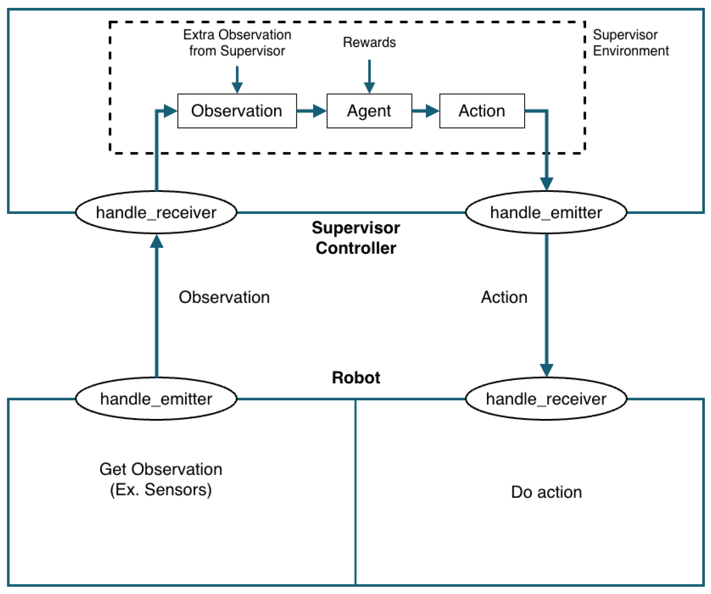
The vehicle controller shown in Figure 7 illustrates how Deepbots, an open-source Python framework, enables a robot control scheme for managing vehicles. The versions of Deepbots and Python are 1.0.0 and 3.9.20, respectively. This setup operates through a supervisory controller, similar to the supervisory framework used in OpenAI Gym, leveraging the observations collected by h a n d l e _ r e c e i v e r to the supervisor controller. The supervisory controller then selects actions based on these observations as calculated by the agent within the supervisory environment. Once a set of actions is chosen, they are transmitted to the robot via the h a n d l e _ e m i t t e r function to execute in the simulation environment. This approach allows researchers to develop a wide range of use cases and utilize them as benchmarks. Additionally, Deepbots serves as a wrapper that encapsulates and simplifies certain operations, allowing users to focus on DRL tasks without getting bogged down by complex simulation details. Furthermore, it enhances the training pipeline with real-time monitoring features, providing researchers with timely insights into essential aspects of the training process. Together, these functionalities create a robust DRL-focused abstraction over Webots, empowering researchers to rapidly develop various use cases and simulation environments while fostering the advancement of sophisticated DRL algorithms [44].
The integration of a first-order Control Lyapunov–Barrier Functions with Proximal Policy Optimization and Higher-Order Control Lyapunov–Barrier Functions with Quadratic Programming, as illustrated in Algorithm 1, facilitates slip angle and acceleration control in autonomous vehicles. Furthermore, the inclusion of a second-order Control Lyapunov–Barrier Functions paired with quadratic programming enhances acceleration control, as detailed in the agent section of Figure 7. This innovative approach effectively combines both learning-based and mathematically driven methodologies, empowering the agent to adeptly navigate emergency pedestrian-avoidance scenarios that frequently arise in real-world driving situations. The learning-based component leverages a "trial-and-error" mechanism to adapt to the complexities of environmental dynamics, utilizing the power of neural networks to efficiently process and compress high-dimensional data. This capability enables the algorithms to handle large datasets and respond swiftly to fluctuations in environmental conditions, showcasing their impressive adaptability. However, in situations where real-time safety is paramount, the mathematically based approach serves a critical role, providing rapid calculations essential for safe driving decisions in immediate, high-pressure circumstances. By ensuring swift and reliable responses, this framework significantly enhances safety and stability for autonomous driving. The synergy between these two methodologies not only guarantees robust performance but also fosters a safer driving experience, particularly in the context of pedestrian avoidance. This paper, therefore, presents a compelling case for the integration of both learning-based and mathematically based algorithms in ensuring safe and efficient autonomous driving.
Algorithm 1 Integration of First-Order Lyapunov–Barrier Function-Proximal Policy Optimization with Higher-Order CLBF-QP
  • Initialize experience replay pool P, experience replay batch η , epoch K, step per episode s, discount factor γ , GAE factor λ , and episode T
  • Initialize Δ = 0 , p = 1
  • Initialize actor - critic network T , T ^ with random weight θ , θ ^
  • Initialize d l , d s , d p
  • Initialize 1st-Order CLBF parameters
  • Initialize 2nd-Order CLBF parameters
  • for episode = 1,T do
  •       reset environment
  •       for step = 1,s do
  •             extract vehicle and obstacles dynamics
  •             select slip control from actor network T ( u β ) and convert to steering angle ( u δ )
  •             optimize acceleration from the HOCLBF-QP ( u a )
  •             calculate the step reward r and next step s
  •             store tactical transition ( s , u β , r , s )
  •             if exp. buffer == P then
  •                   for epoch = 1,K do
  •                          random the experience samples η
  •                          calculate GAE advantage from Equation (28)
  •                          calculate modified 1st-order CLBF advantage estimator from Equation (30)
  •                          update actor network weight θ by actor loss from Equation (31)
  •                          update critic network weight θ ^ by critic loss from Equation (32)
  •                   end for
  •             end if
  •             if done then
  •                   store tactical transition ( s , u β , r , s )
  •                   trigger the reset flag
  •             end if
  •        end for
  • end for
In this experiment, the controller runs at a fixed control period of 40 ms, i.e., a control rate of 25 Hz: at each step, the trained policy is queried for the slip-angle command and the HOCLBF-QP of equation Equation (37) is solved once for the acceleration command before the action is applied to the vehicle.

4. Simulation Result and Discussion

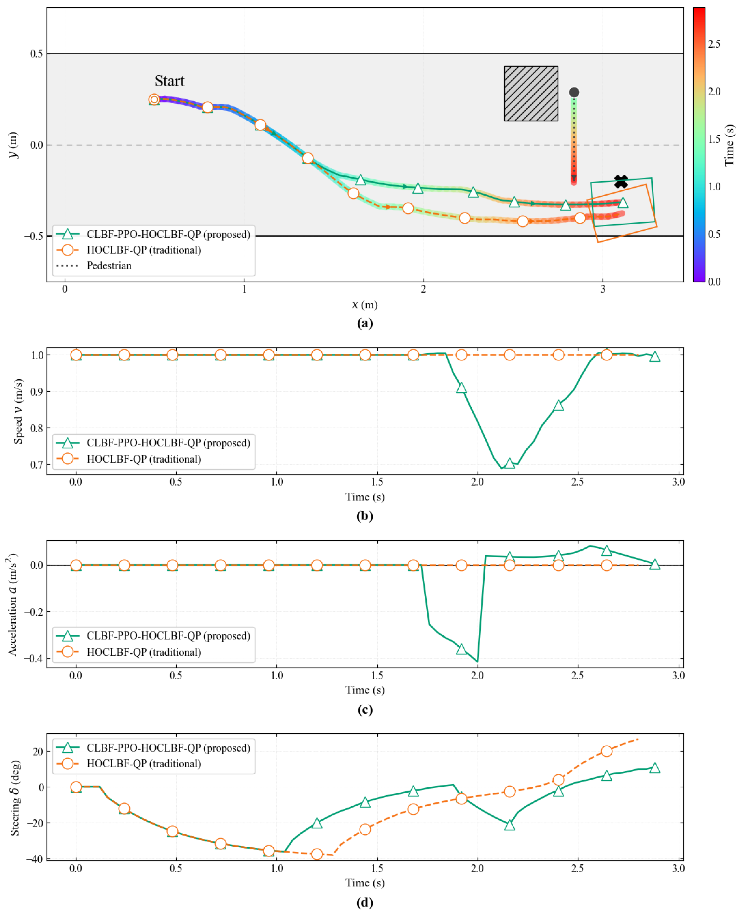
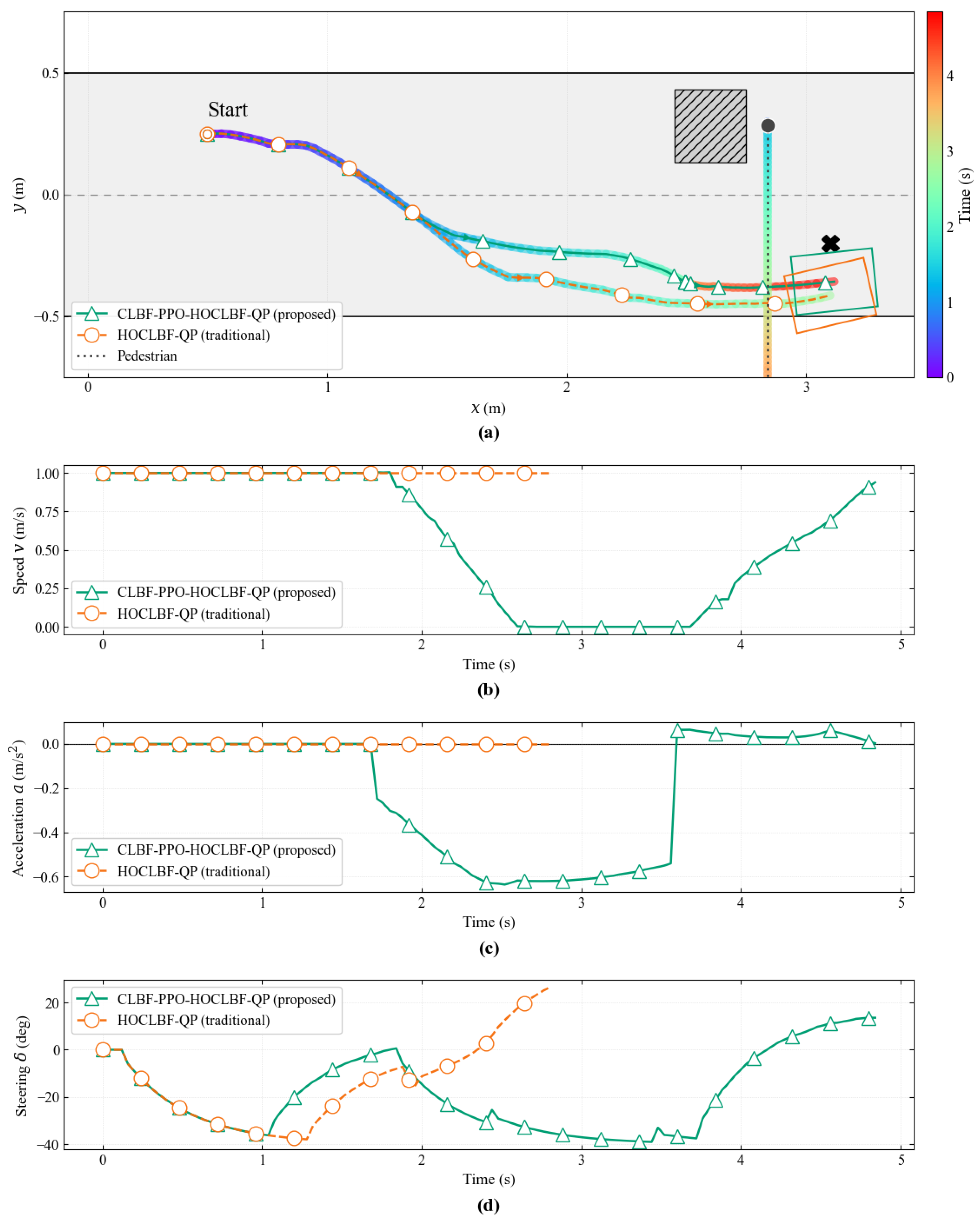
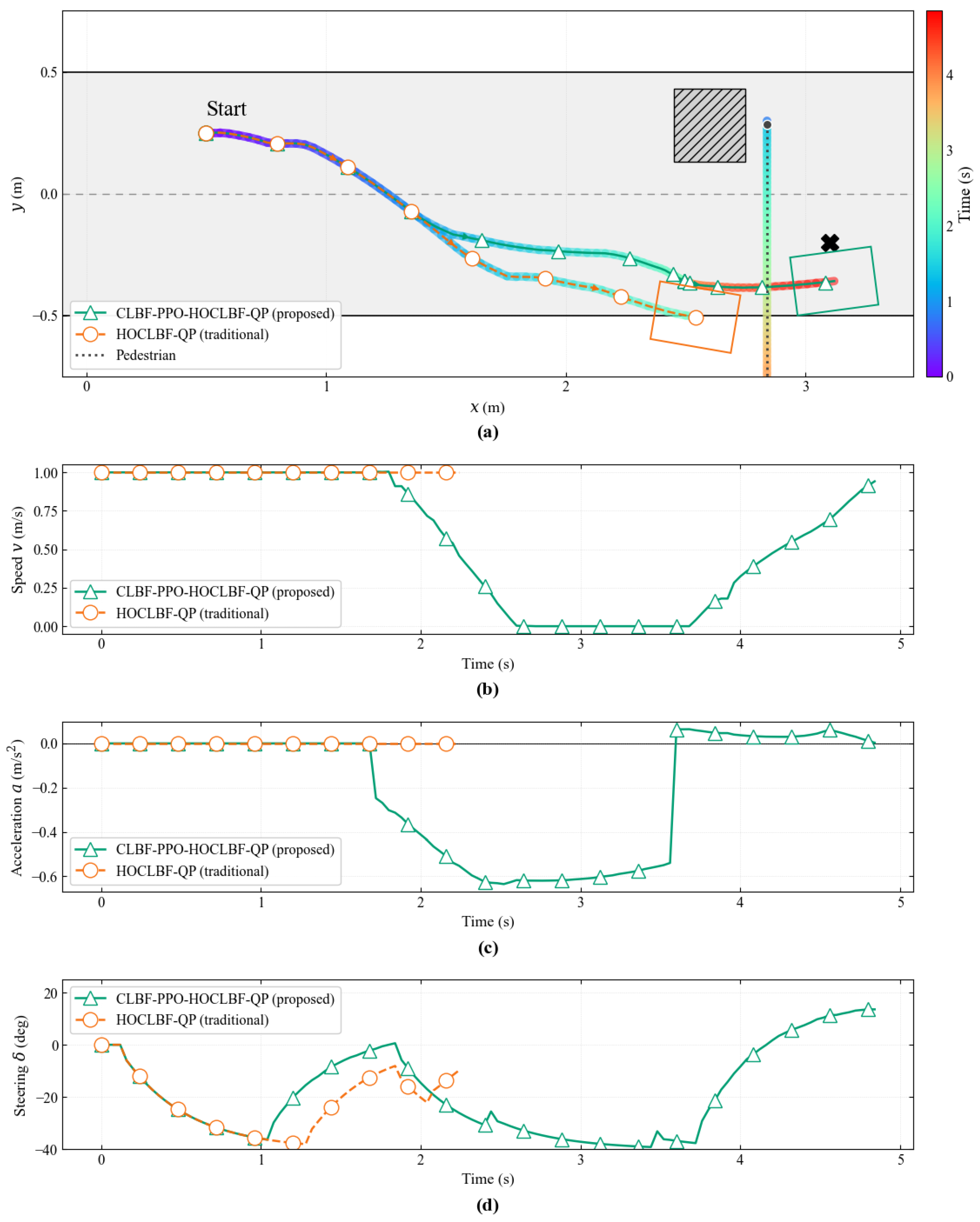
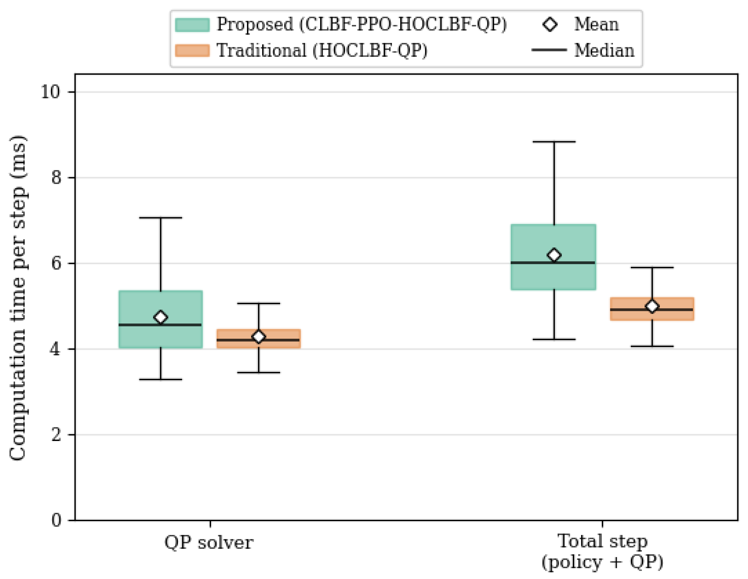
This section presents the simulation results and discussion of the proposed framework, organized into four parts. Section 4.1 examines how the 1st-order CLBF advantage modifier influences Proximal Policy Optimization during training, analyzing the effect of the control Lyapunov weight d l , the static-obstacle barrier weight d s , and the pedestrian barrier weight d p on the agent’s learning, and comparing the resulting policy against the PPO(MLP) and PPO-LSTM baselines. Section 4.2 then studies the deployment-time HOCLBF-QP layer, investigating how the class- K coefficients shape the agent’s braking response to a crossing pedestrian and its goal-reaching behavior. Section 4.3 compares the integrated CLBF-PPO-HOCLBF-QP framework against the traditional HOCLBF-QP baseline across a range of pedestrian crossing speeds. Finally, Section 4.4 reports the per-step computational time of both controllers and assesses the real-time feasibility of the online optimization at the control rate defined in Section 3.3.

4.1. Effect on 1st-Order CLBF Advantage Estimates to Proximal Policy Optimization

This subsection focuses on the impact of the first-order CLBF advantage modifier by varying each of its three weights individually, while keeping the other weights constant. The weights under consideration are: the control Lyapunov weight d l as discussed in Section 4.1.1, the static-obstacle barrier weight d s in Section 4.1.2, and the pedestrian barrier weight d p in Section 4.1.3. For each variation, the resulting training return and agent trajectory will be compared with the corresponding reference setting.
All results in this section are aggregated over three random seeds with three repetitions for each seed; the tables report the mean and standard deviation across runs with a 90% confidence interval, and the exploration-entropy setting is given in Table A1. The episodic return curves are shown as a 50-episode moving average, applied solely to improve the legibility of the high-frequency return signal.

4.1.1. Effect on Control Lyapunov Weight d l on Agent’s Learning

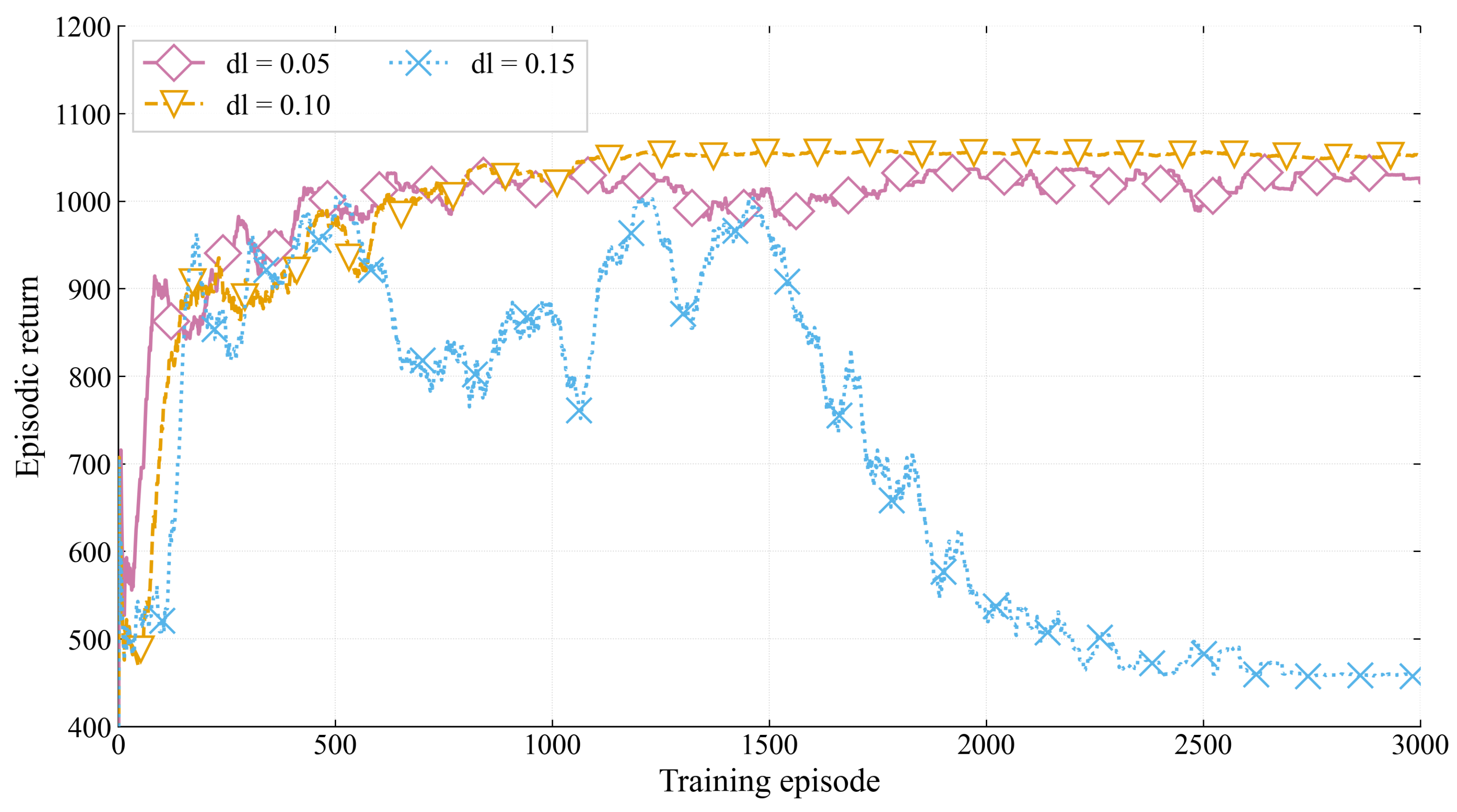
Following the modified advantage estimates by CLF, Figure 8 compares the episodic return over training under different Control Lyapunov Function weights, where d l = 0.05 is shown as the pink triangle line, d l = 0.10 as the light-orange downward-triangle line, and d l = 0.15 as the blue cross line. All curves are reported as 50-episode moving averages of the episodic return over the training horizon. In this experiment, the agent only drives to reach the goal, without pedestrian movement, at a full speed of 1 m / s . The return reflects how well the agent learns to complete the scenario over training. Regarding the influence of d l , summarized in Table 2, adding a moderate Lyapunov weight helps the agent learn goal-reaching behavior: for d l = 0.05 and d l = 0.10 , the agent converges to a high return. At d l = 0.05 , the CLF signal on the advantage is strong enough to bias the policy gradient toward goal-converging actions, yet small enough that the GAE advantage term still dominates; this setting converges fastest, with average return at 976.02. At d l = 0.10 , although the convergence is slightly slower, the margin is higher than d l = 0.05 . Moreover, the return trend is the smoothest, indicating the most stable learning, with more than 90% success rate. However, an excessively strong CLF signal, d l = 0.15 , degrades learning: the analytic Lyapunov term begins to overwrite the learned GAE advantage, and because this term is myopic—reflecting only the instantaneous sign of the Lie derivative rather than the long-horizon return—the policy gradient is pulled by a short-sighted signal, training destabilizes, and the agent ultimately fails to reach the goal. The effect of d l is therefore non-monotonic: the CLBF modifier accelerates and stabilizes goal-reaching only within a moderate weight range, where it injects an explicit stability signal without displacing the learned advantage.
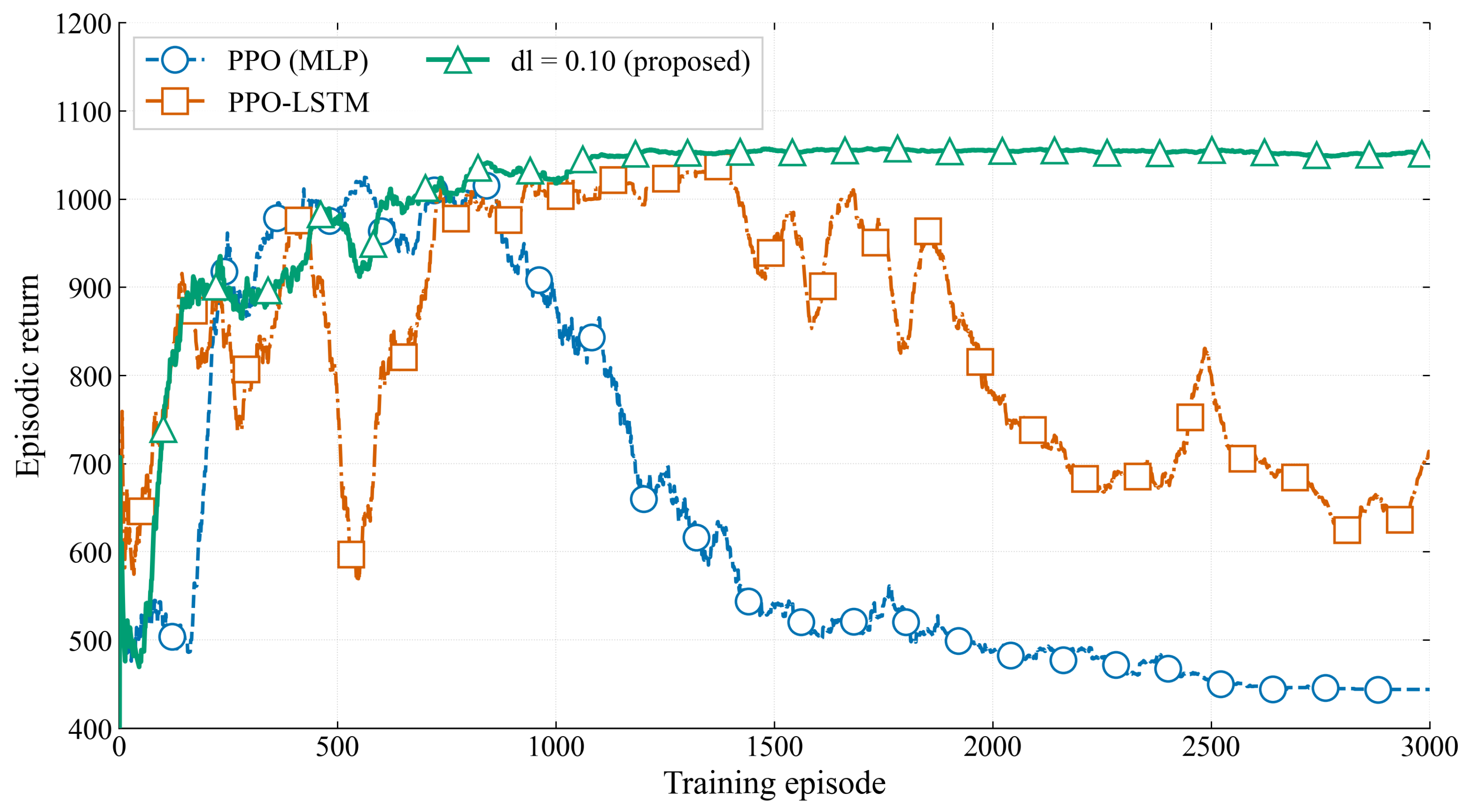
Figure 9 compares baselines: PPO(MLP), represented by the blue dashed circle, and PPO-LSTM, the dark orange squared line from [46], against the proposed method, with a control Lyapunov weight d l of 0.10, on the identical goal-reaching task. The proposed method rises quickly and holds at a high, stable plateau throughout training, while both baseline approaches reach a comparable early peak and then decline; PPO-LSTM oscillates and fails in later episodes, and PPO(MLP) steadily collapses to the lowest returns by the end of training. This contrast follows directly from the modified advantage estimate in Equation (30). The baselines drive the policy gradient using only the GAE advantage, which is bootstrapped from a still-learning critic. Once the agent explores away from the goal-reaching behavior, no structural signal pulls it back, and the policy drifts. Instead, the proposed approach adds the CLF term, computed from the analytic Lie derivative of the Lyapunov function and therefore independent of the critic value, which at every update re-penalizes actions that violate the CLF descent condition and continually steers the policy toward goal-reaching actions. Because PPO-LSTM is the more capable baseline, it has recurrent memory and additional parameters inside. However, the learning still degrades. The improvement cannot be attributed to network capacity, but specifically to the explicit stability signal injected by the first-order CLBF advantage modifier.
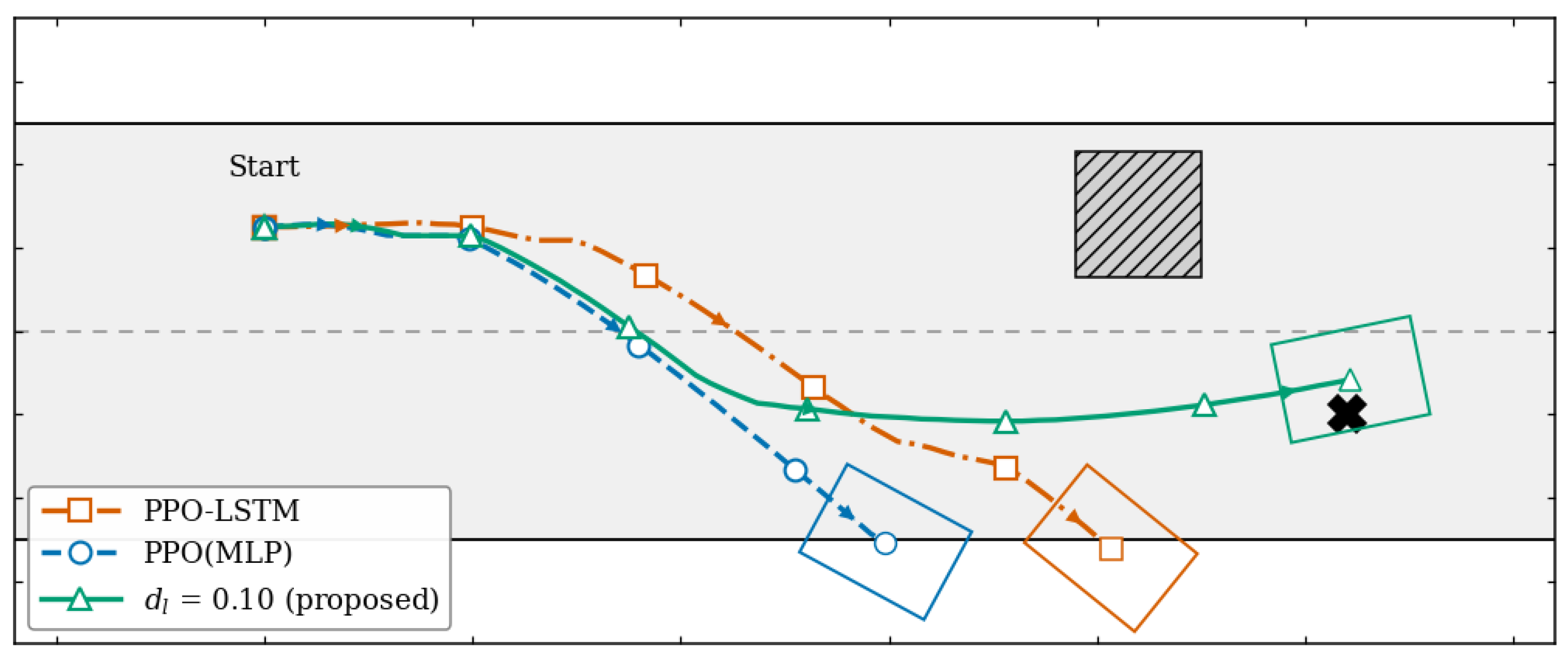
In terms of agent trajectory, Figure 10 illustrates the trajectories for the three controllers on a similar goal-reaching task. The proposed method at d l = 0.10 (green dashed-dot line) conducts a smooth, continuous path that curves around the static obstacle (box) and terminates at the goal region, with the agent’s final pose aligned to the goal. Whereas both baselines fail to complete the scenario: the PPO-LSTM trajectory (blue) advances further than PPO(MLP) but stalls short of the goal, while the PPO(MLP) trajectory (orange dashed) deviates from the goal-directed path earlier and terminates before reaching the goal. These trajectories are the spatial matching of the return curve in Figure 9. In the CLF descent signal, it keeps the agent’s heading toward the goal throughout the episode, whereas the baselines, lacking that structural anchor, drift off the goal-reaching path once their learned policy degrades.

4.1.2. Effect on Control Barrier Weight on Static Obstacle d s on Agent’s Learning

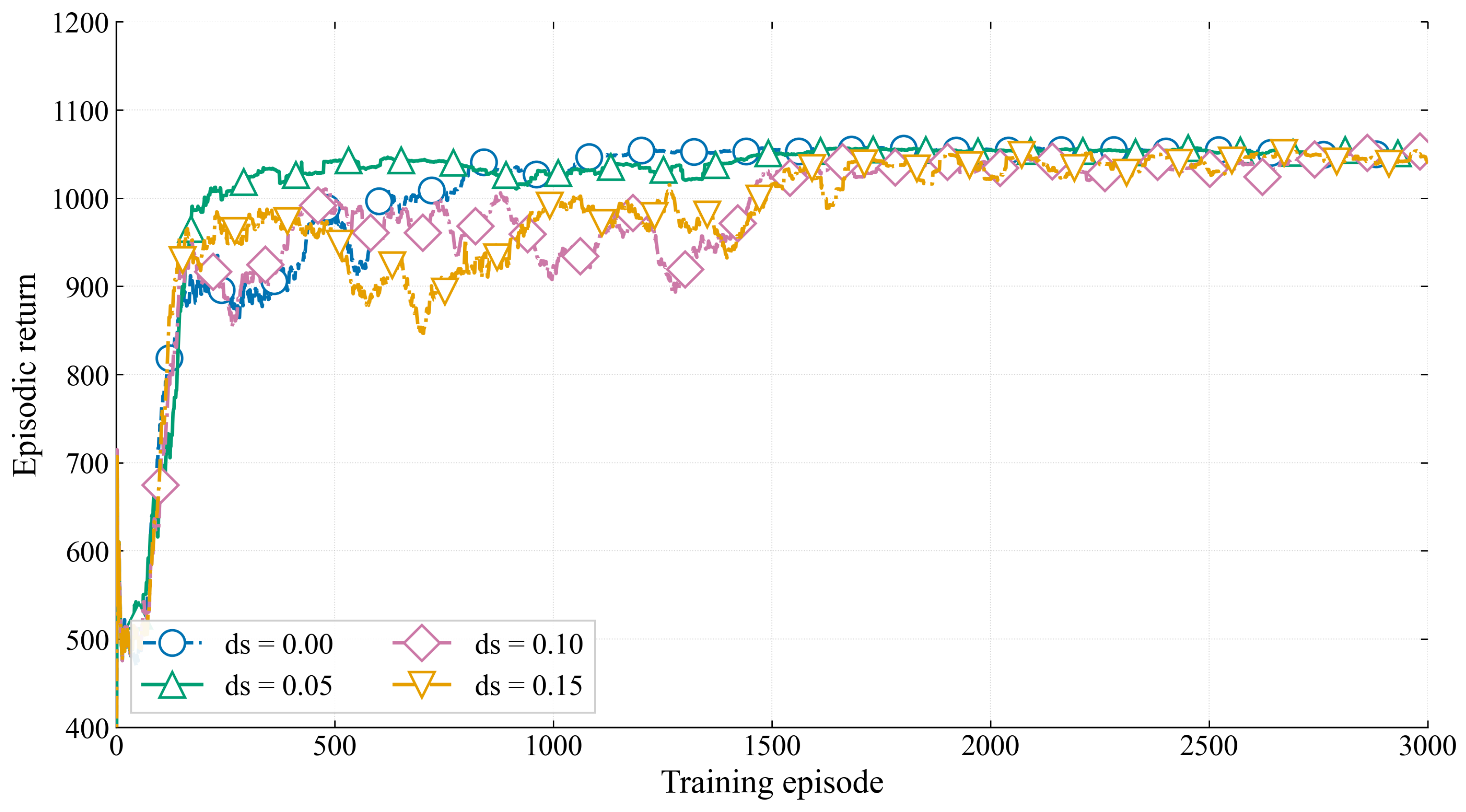
Regarding the influence of the Control Barrier Function weight d s on agent training, and under the same conditions as the control Lyapunov weight experiment—the absence of a pedestrian and a fixed agent speed of 1 m / s Figure 11 illustrates how the barrier weight on the static obstacle (the box) affects the agent’s training, with the Lyapunov weight held fixed at d l = 0.10 ; the d s = 0.00 case therefore coincides with the control-Lyapunov-only reference. At d s = 0.05 (green triangle line), the inclusion of the barrier weight accelerates the agent’s learning relative to the unweighted case and yields a more stable learning process, and Table 3 shows that it raises the success rate above the unweighted baseline at an essentially unchanged average return. As the barrier weight is increased further, to d s = 0.10 and d s = 0.15 , performance deteriorates: the success rate declines below the unweighted baseline and the training return converges more slowly. As reported in Table 3, the average advantage decreases monotonically with d s , since the barrier penalty only subtracts from the advantage and a larger weight further attenuates the dominant GAE term. The decline in success rate is instead caused by an overly conservative policy: at d s = 0.15 , the agent maintains an unnecessarily large clearance from the obstacle and continues to accumulate step-wise safety and proximity rewards yet fails to reach the goal reliably. The influence of d s is therefore non-monotonic, mirroring that of d l : a moderate barrier weight accelerates and stabilizes learning while improving obstacle avoidance, whereas an excessive weight sacrifices goal-reaching in favor of over-cautious behavior. The two ablations are distinguished only by their failure modes—an over-weighted d l destabilizes training, whereas an over-weighted d s preserves training stability but renders the policy over-conservative.
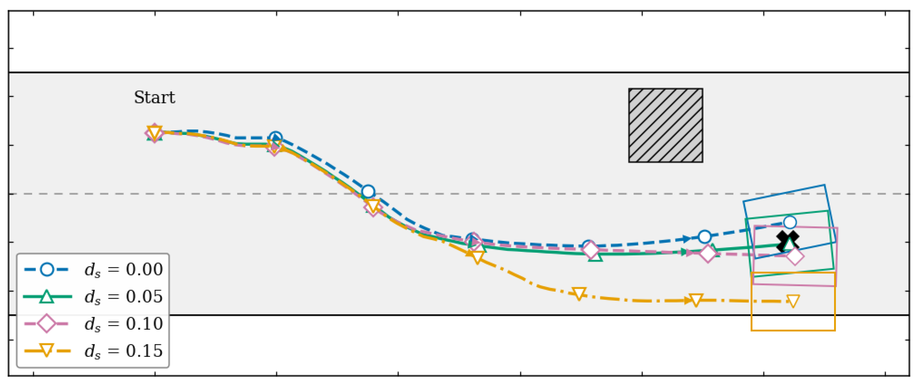
Figure 12 depicts the agent’s trajectories over the barrier weight on a static obstacle. Because d s scales the penalty on any steering action that reduces clearance to a wider position, for most of the values, from d s = 0.00 to d s = 0.10, the trajectories remain closely clustered, with slight separation from the box, each rounding the box along a smooth, goal-directed path and terminating at the goal with the agent aligned to the target. However, at d s = 0.15, the trajectory markedly departs from the others, swinging into a much wider, lower arc that keeps an excessive distance from the box and deviates from the goal-reaching route, so that the agent may drive off the road rather than staying on the road; this is thus the drop in the success rate. A moderate d s yields a path that is safe yet still goal-directed, whereas an excessive d s produces an exaggerated route in which obstacle clearance is prioritized over goal-reaching. The agent continues to grow stepwise safety and proximity rewards across its wide area, but no longer reliably reaches the goal.

4.1.3. Effect on Control Barrier Weight on Pedestrian d p on Agent’s Learning

In this study, we investigated the impact of control barrier weight on the training efficacy in pedestrian avoidance scenarios. We simulated a situation in which a pedestrian at a crosswalk is obscured by a box, rendering them invisible to the agent. The pedestrian’s movement speed is set at 0.325 m / s , while the agent’s maximum speed is equal to 1 m / s .
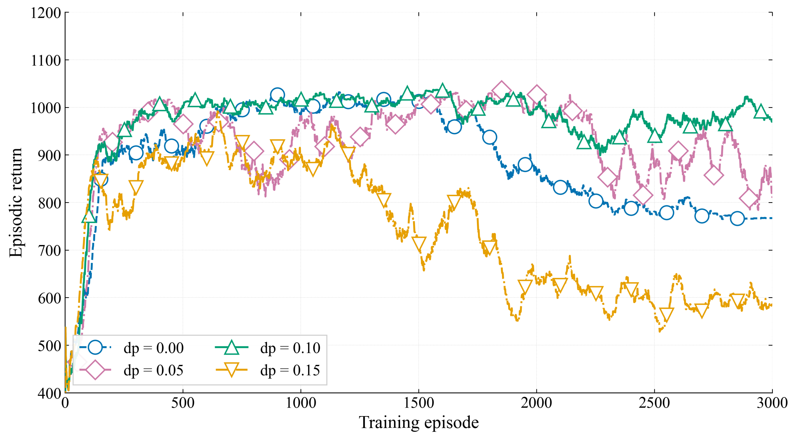
As illustrated in Figure 13, in the scenario where no weight is applied (i.e., the unweighted case), the reward achieves an initial peak but subsequently declines and plateaus throughout the training period, resulting in a success rate that remained below 50%. This trend indicates an insufficient signal from the pedestrian barrier, which hampers the policy’s development.
Increasing the pedestrian barrier weight, denoted as d p , significantly improves training performance through enhanced penalties for pedestrian safety derived from Lie derivatives. Specifically, at weights of d p = 0.05 and d p = 0.10 , the training performance improves; however, the lower weight of d p = 0.05 introduced considerable oscillations in the reward, leading to inconsistencies in the learning signal regarding pedestrian avoidance. In this instance, a stronger signal facilitates a more stable learning trajectory, resulting in elevated average returns and an increased success rate, allowing the agent to learn pedestrian avoidance more effectively.
Conversely, excessive weight may compromise the training process. Similar to the unweighted scenario, an excessive weight of d p = 0.15 exhibits a similar trajectory, experiencing an initial peak followed by a drop into a low reward band. The observed weight dynamics reflect the significance of maintaining a coherent learning environment; weights of d p = 0.05 and d p = 0.10 successfully sustained a high, stable performance plateau once peak performance is achieved. In contrast, the absence of a signal (at d p = 0.00 ) and the application of excessive weight (at d p = 0.15 ) both fail to maintain this plateau. The former case lacks an adequate structural signal to mitigate policy drift, while the latter suffers from a myopic analytic term that progressively overshadowed the learned advantages.
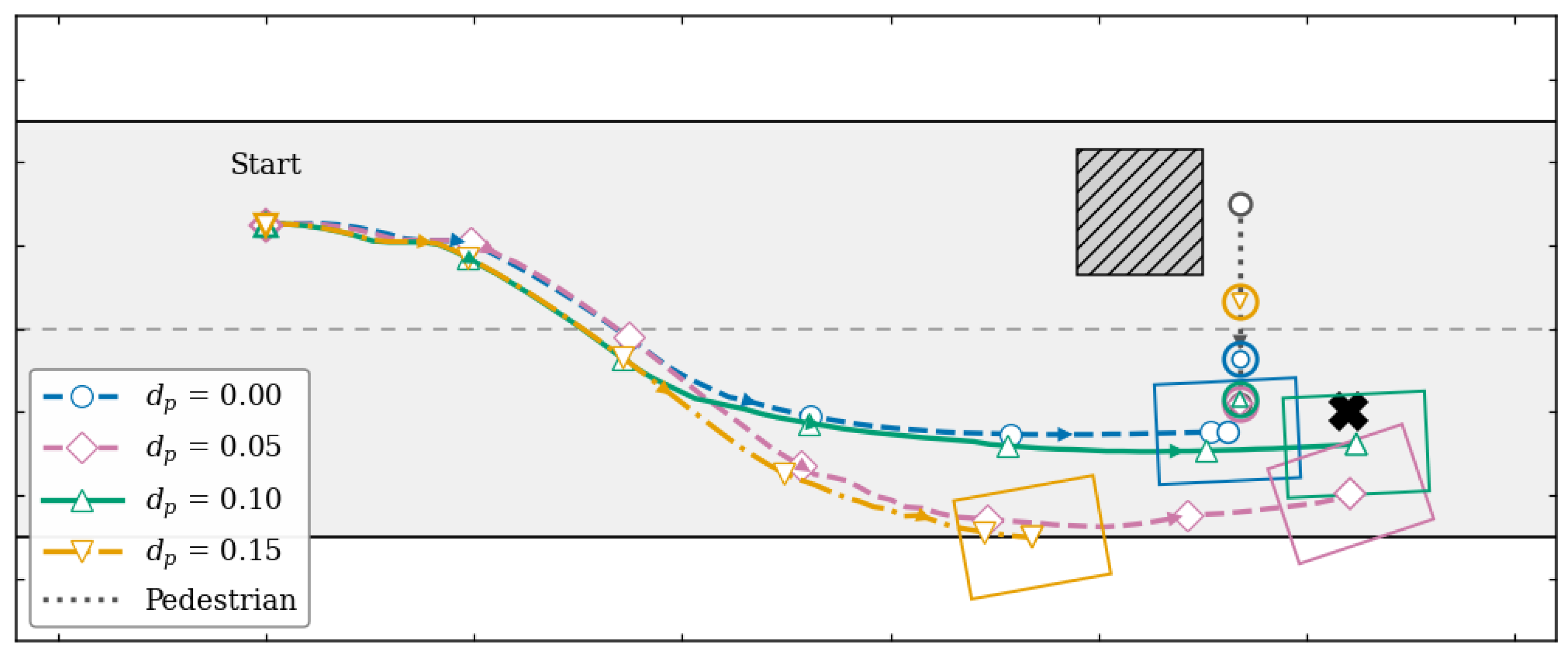
Figure 14 illustrates the spatial trajectories of the agent with varying weights assigned to the pedestrian barrier variable ( d p ). These trajectories reflect the return trends observed in Figure 13 and the quantitative results presented in Table 4. This is the first trajectory comparison conducted with a pedestrian actively crossing, and the figure depicts the static obstacle, the pedestrian, and the path the agent takes as it emerges from behind the occluding obstacle.
At d p = 0.00 , the reference trajectory results in a collision with the pedestrian during training. Without a pedestrian barrier term in the modified advantage estimate, the policy lacks an explicit avoidance signal, causing the agent to drive directly into the pedestrian’s path. This behavior aligns with the low success rate of 49.80% recorded for this configuration.
When the pedestrian barrier signal is activated, the agent’s behavior changes significantly. At both d p = 0.05 and d p = 0.10 , the agent successfully steers away from the pedestrian and reaches the goal region, completing the scenario. However, the quality of the resulting path varies between the two settings. At d p = 0.05 , the trajectory is comparatively irregular, showing a tendency to drift toward the road boundary. This indicates a reduced safety margin, consistent with its success rate of 73.83% and the greater oscillation noted in Figure 13. In contrast, at d p = 0.10 , the stronger emphasis on pedestrian barrier awareness produces a significantly smoother and better-centered trajectory that consistently reaches the goal, correlating with the highest success rate of 78.07%. When the weight is further increased to d p = 0.15 , the agent overreacts to the barrier signal, veers off the road, and fails to complete the scenario, resulting in a sharp decline in success rate to 30.47%.
Regarding the agent’s trajectory, it thus confirms that the intensity of the pedestrian barrier weight directly influences the agent’s driving behavior. An insufficient weight provides no collision-avoidance capability and leads to accidents, while a moderate weight results in a safe, goal-directed path—most effectively at d p = 0.10 . Conversely, an excessive weight causes the agent to stray off the road. This non-monotonic relationship is consistent with the effects of d l and d s observed in previous ablations and confirms that the pedestrian barrier modifier enhances driving behavior only within a moderate weight range.

4.2. Effect on HOCLBF-QP Optimization on Acceleration–Brake Algorithm in Driving Behavior

This subsection transitions from training to deployment, focusing on how the class- K coefficients of the HOCLBF-QP filter influence the agent’s behavior in real-time, particularly when encountering a crossing pedestrian. In Section 4.2.1, we analyze the barrier coefficients α p , 1 and α p , 2 , which control the braking response. Meanwhile, Section 4.2.2 discusses the Lyapunov coefficients α l , 1 and α l , 2 , which manage the goal-reaching process once the pedestrian has cleared the path.

4.2.1. Influence of the Coefficients of α p , 2 and α p , 1 on Pedestrian Braking Behavior on the HOCBF-QP

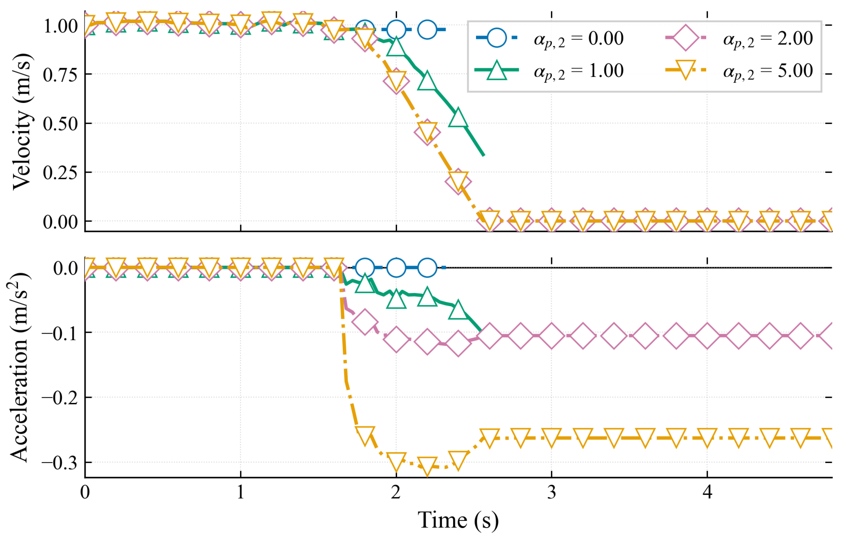
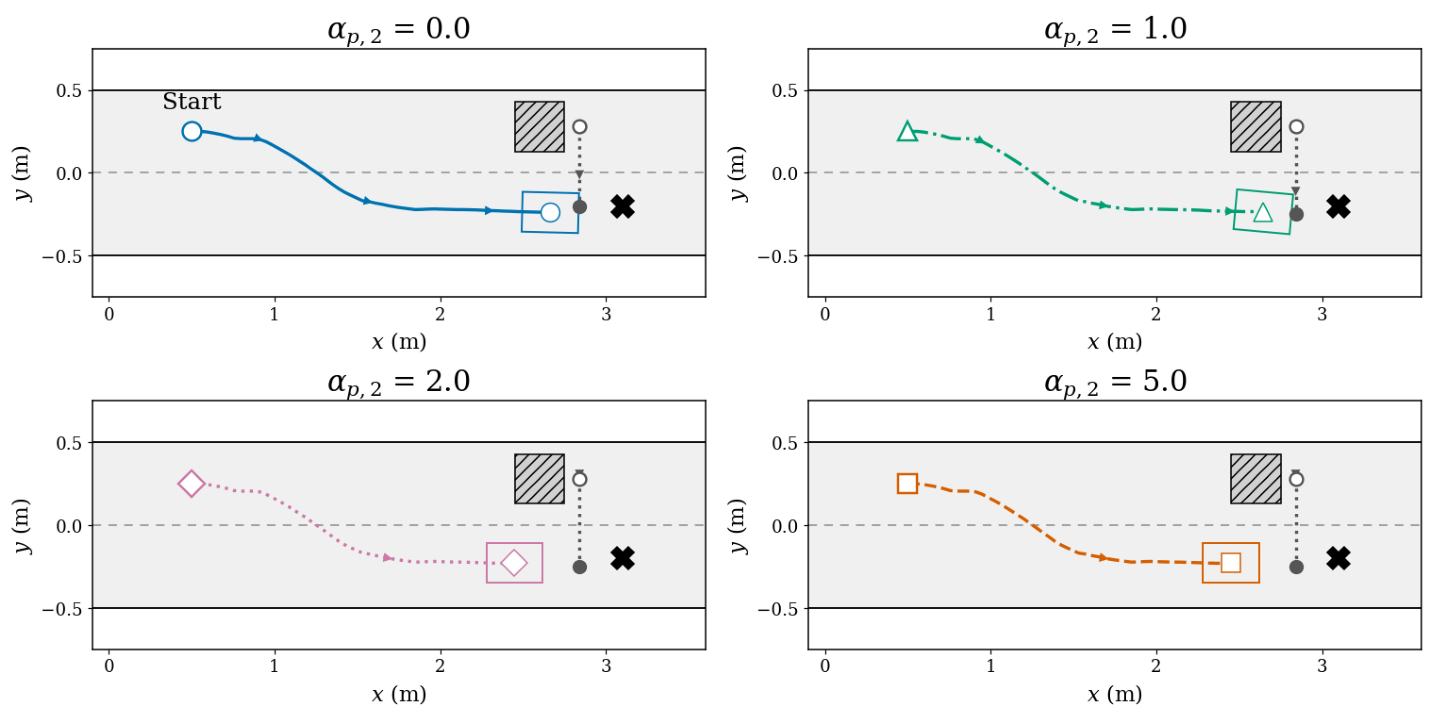
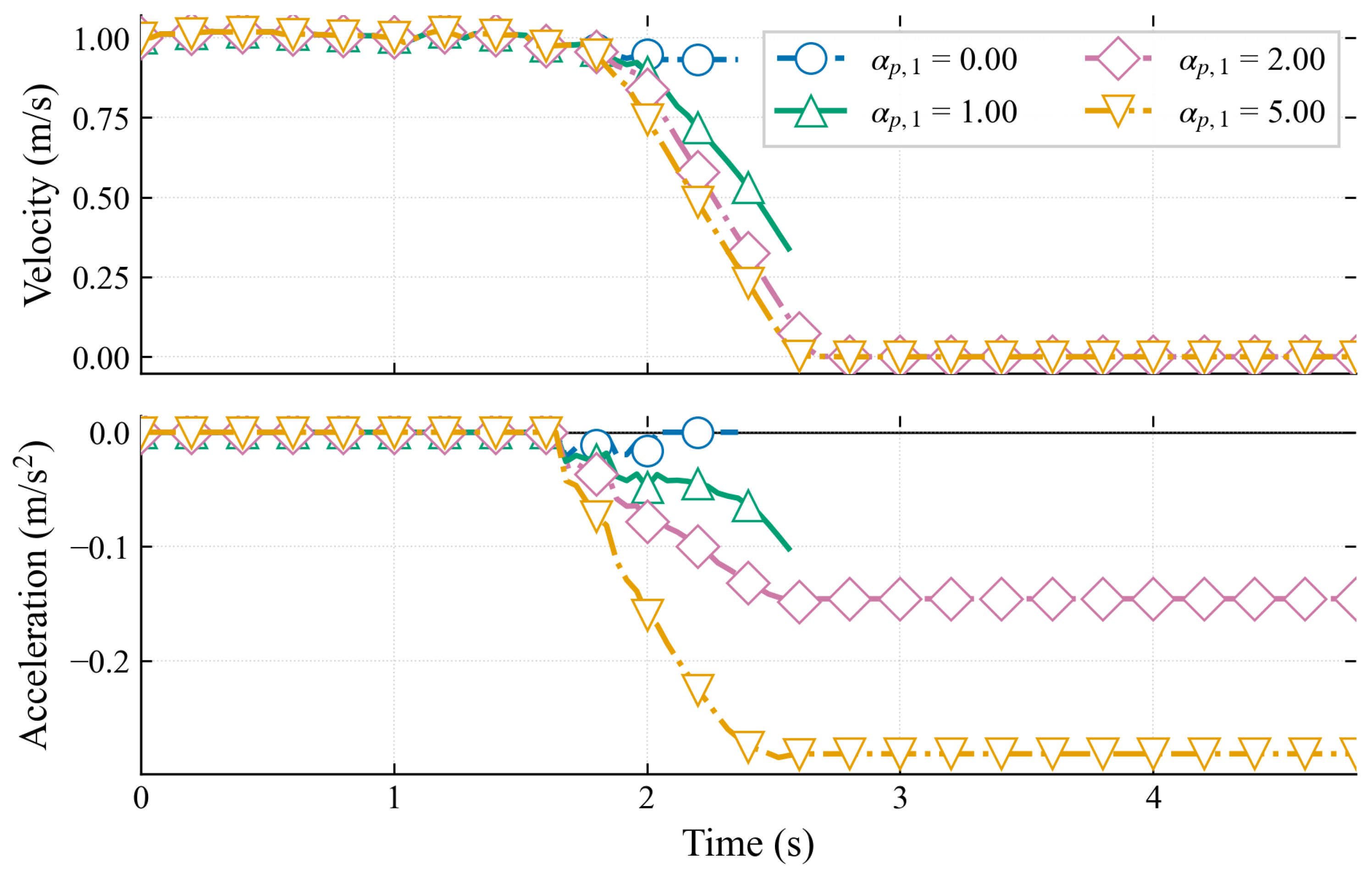
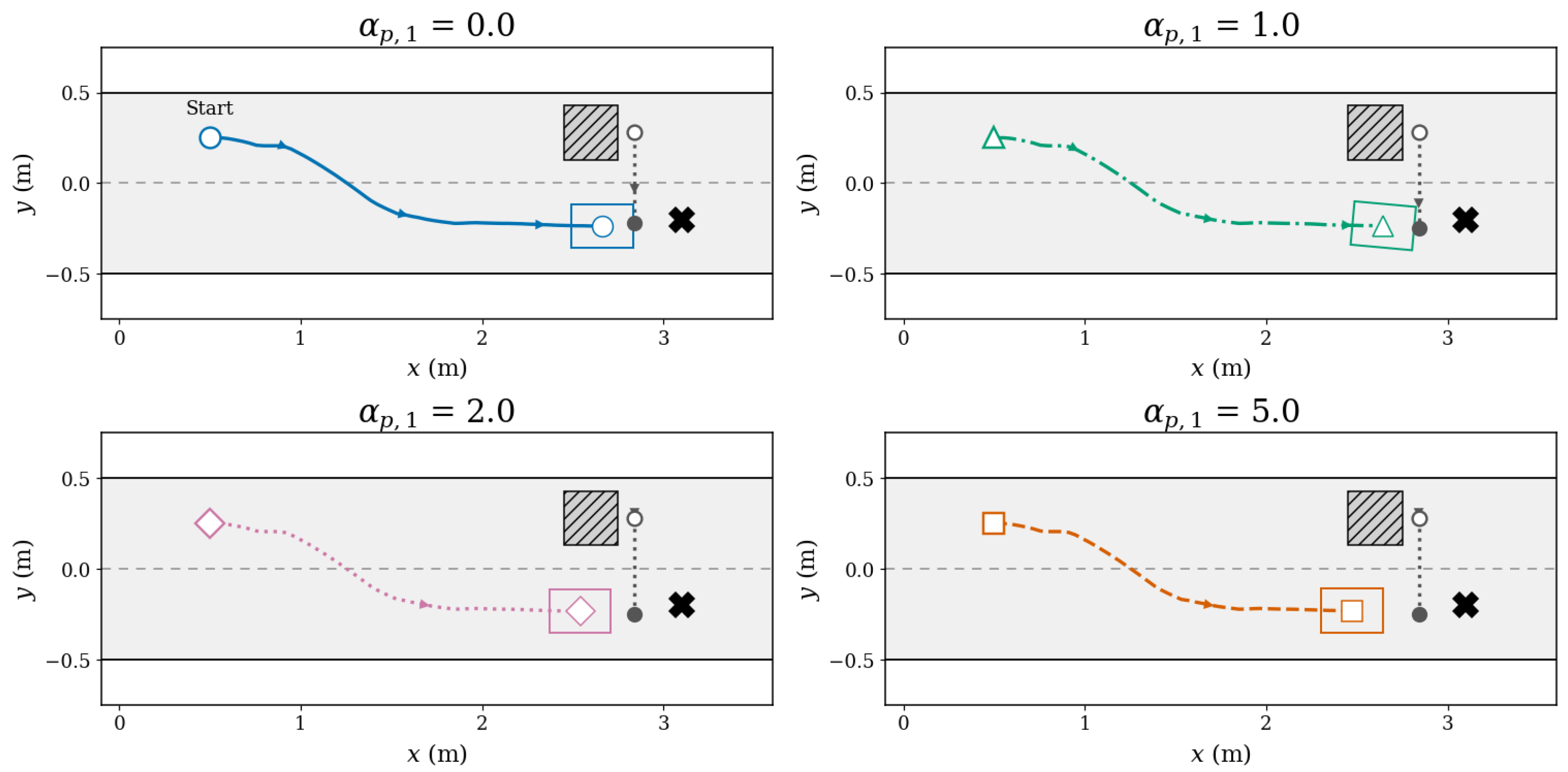
The analysis of safety behavior in the HOCBF-QP with respect to pedestrians is depicted in Figure 15, Figure 16, Figure 17 and Figure 18. These figures show the agent’s braking actions, velocity, acceleration, and the resulting trajectories as influenced by the coefficients α p , 1 and α p , 2 in the HOCBF, as described in Equation (24). In this study, we simulate a situation where the agent, which employs slip angle control based on a trained model with weights set at d l = 0.10 , d s = 0.05 , and d p = 0.10 , travels at a speed of 1 m / s toward a goal. At the same time, a pedestrian crosses the road at 0.5 m / s and is located in the center of the right lane. This scenario resembles a pedestrian walking who suddenly trips. Additionally, we set the value of K p in (37) to 100.0.
According to the HOCBF equation, when α p , 2 is zero, the agent does not initiate braking. The QP keeps the nominal acceleration unchanged, causing the agent to continue at its current speed without applying the brakes, even as it nears the pedestrian. This lack of controlled deceleration results in a violation of the safety margin, illustrating that the higher-order barrier term is what drives the avoidance maneuver, rather than the nominal policy.
When the coefficients are non-zero, the QP adjusts the nominal acceleration to remain within the safe limits, prompting the agent to decelerate. The distinction between settings, however, is clearest in the velocity profile rather than in the peak deceleration alone. At α p , 2 = 1.00 , the barrier term is too weak to enforce timely braking: deceleration begins late and stays shallow (a peak of about 0.1 m / s 2 ), so the agent’s speed falls too gradually and does not reach zero before the gap to the pedestrian closes, resulting in a collision. When α p , 2 is increased to 2.00, the braking onset is earlier and sharper, and the velocity is driven to zero before the vehicle reaches the pedestrian. Hence, the agent halts in time, and avoidance succeeds. Increasing α p , 2 further to 5.00 produces the steepest profile, with the peak deceleration rising to roughly 0.3 m / s 2 and the vehicle stopping soonest. The trend is therefore monotonic in α p , 2 but the decisive difference between collision and avoidance at moderate gains lies in when braking begins and whether the speed is brought to zero in time—both governed by the closing-rate term L f h ( x ) , which captures the relative velocity between the vehicle and the moving pedestrian. For this reason, α p , 2 regulates the strength, sharpness, and onset of the braking response, linking it more closely to the closing speed than to the absolute distance. The corresponding trajectories under each α p , 2 setting are shown in Figure 16. Figure 18 presents the trajectories when α p , 1 is varied with α p , 2 fixed at 1.00, exhibiting the same qualitative pattern.

4.2.2. Influence of the Coefficients of α l , 2 and α l , 1 on Goal-Reaching Behavior on the HOCLF-QP

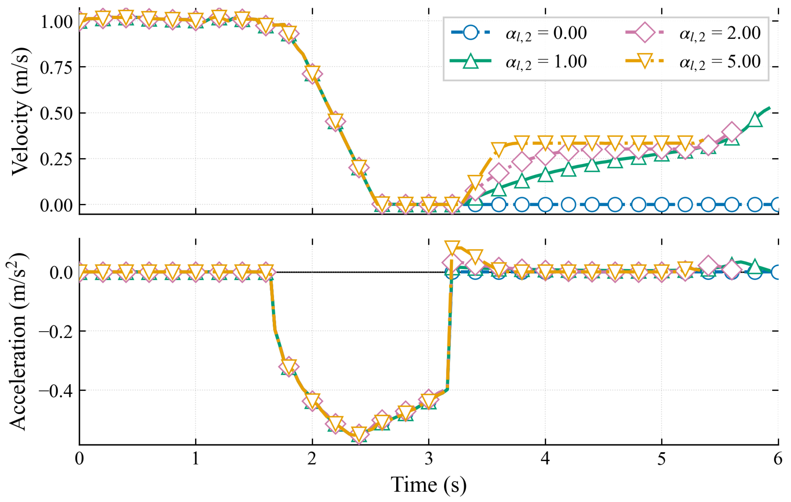
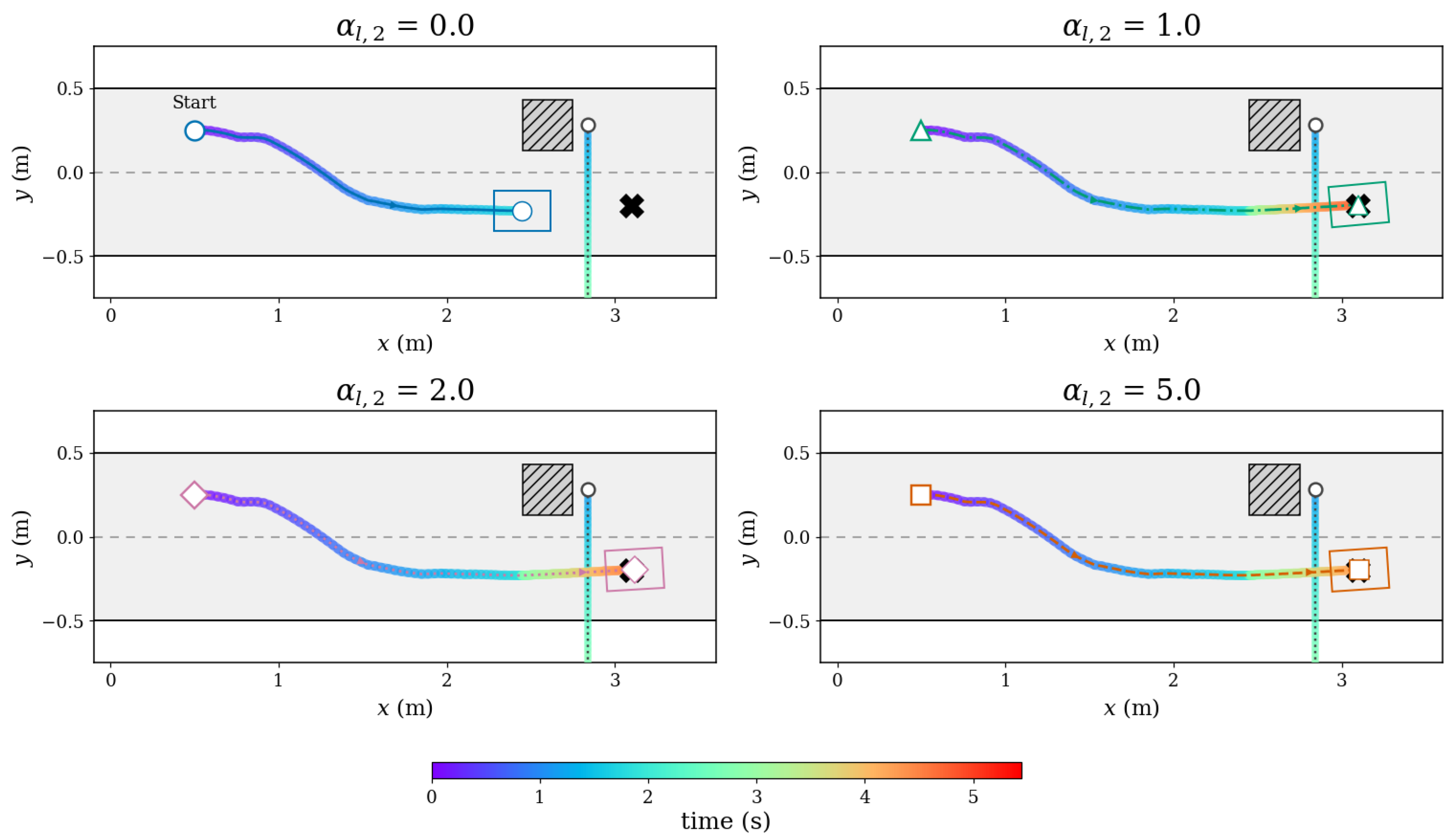
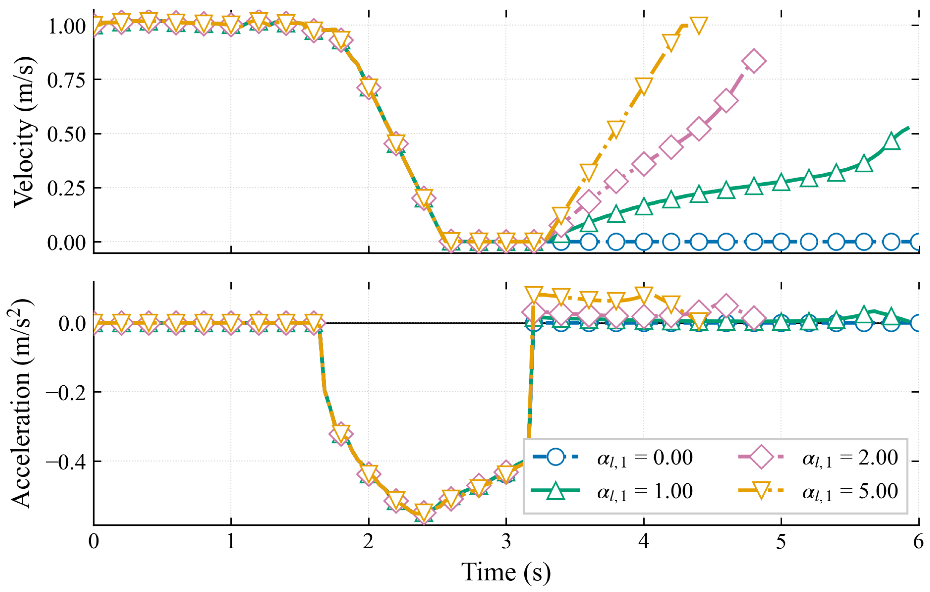
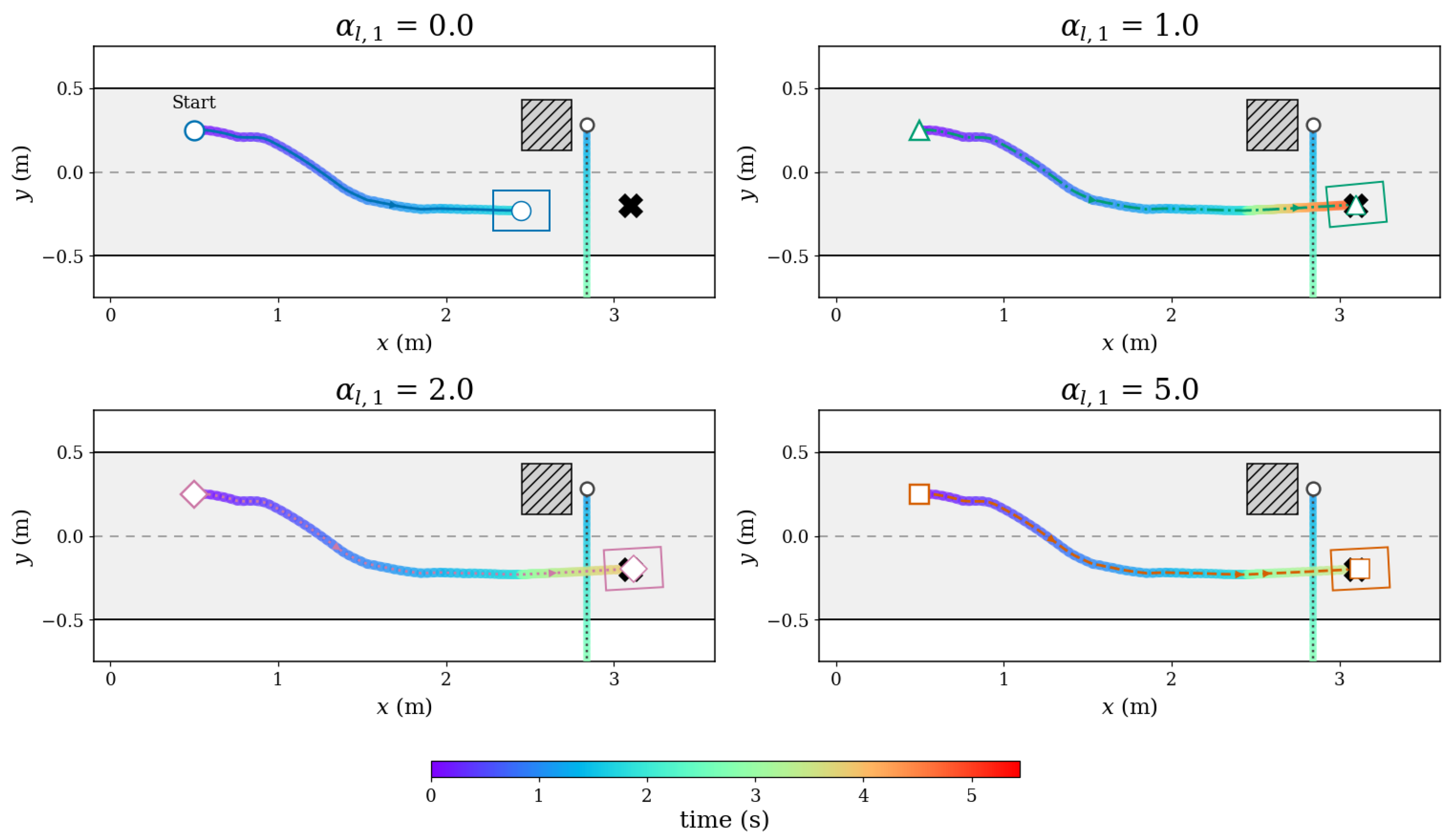
In the goal-reaching approach applied to the HOCLF-QP framework, as illustrated in Figure 19, Figure 20, Figure 21 and Figure 22, we examine the effects of the parameters α l , 2 and α l , 1 on the agent’s behavior in reaching its goal. In our experiment, we simulate a scenario where the agent navigates a roadway with a pedestrian moving across the street at a constant speed of 0.5 m / s . Regarding the weights K l , K p in Equation (37), we set K l to 10.0 and K p to 100.0, similar to the experiments conducted in the pedestrian braking scenario.
Regarding the influence of α l , 2 detailed in Figure 19, which relates to (18) and (37), we observe that when α l , 2 is set to 0.00, the agent comes to a complete stop after braking and remains stationary. Without a state-dependent convergence signal from the CLF constraint, the agent does not regain motion, demonstrating that the higher-order Lyapunov term, rather than the standard policy, is responsible for driving the goal-reaching behavior. Conversely, for any non-zero values of α l , 2 , the QP effectively promotes convergence, and the agent actively seeks to reach the goal. The responsiveness of the maneuver varies with the parameter; specifically, the velocity directed toward the goal is influenced by the goal-closing rate L f V ( x ) . Additionally, since this gain directly affects the acceleration input, a larger α l , 2 yields a more pronounced corrective acceleration, resulting in a quicker approach to the goal—with α l , 2 set to 5.00 leading to the fastest convergence and 1.00 yielding the slowest among the non-zero values. Thus, α l , 2 dictates the intensity and precision of the corrective actions, linking the agent’s response to the closing speed rather than just the absolute distance to the goal. The corresponding time-coded trajectories are shown in Figure 20.
On the other hand, the effects of α l , 1 on goal-reaching behavior are demonstrated in Figure 21. With α l , 1 set to zero, the agent behaves similarly to cases where α l , 1 is unweighted, as the distance-dependent term V ( x ) is effectively removed. When α l , 1 obtains a weight, it introduces a distance-dependent convergence, scaling the position error V ( x ) and determining the aggressiveness with which the agent reduces this error based on the remaining distance to the goal. As α l , 1 increases, this term becomes increasingly significant in the constraint, enabling stronger convergence and allowing the agent to close the error over a shorter time frame; conversely, the smallest non-zero weight results in the slowest convergence. Hence, α l , 1 plays a critical role in how cautiously the agent manages its approach in relation to the remaining distance to the goal. Figure 22 shows the corresponding trajectories.

4.3. Comparison on Integration of the First-Order Lyapunov—Barrier-Proximal Policy Optimization and Higher-Order CLBF-QP and Traditional Higher-Order CLBF-QP in Agent’s Driving Behavior in Various Pedestrian Speed

This subsection illustrates a comparison of the agent’s driving behaviors in a scenario involving pedestrians crossing at various speeds. The agent, starting with an initial speed of 1.00 m / s , drives toward its goal while responding to pedestrians moving at constant speeds of 0.325 m / s , 0.425 m / s , and 0.500 m / s . These comparisons are depicted in Figure 23, Figure 24 and Figure 25, respectively, and Table 5 consolidates the comparison into a single set of quantitative metrics, grouped into safety-and-avoidance, goal convergence, kinematic-model validity, and QP constraint relaxation. The CLBF-PPO model is employed, trained with a fixed Control Lyapunov–Barrier controller, with parameters set to d l = 0.10 , d s = 0.05 , and d p = 0.10 for the training policy. Additionally, the HOCLBF-QP parameters are defined as α l , 1 = 2.0 and α l , 2 = 2.0 for the HOCLF-QP based on Equation (19). For the HOCBF-QP, the parameters are set to α p , 1 = 5.00 and α p , 2 = 2.00 based on Equation (24). The slack weight is K l = 10.0 and K p = 100.0 in the QP optimization according to Equation (37). In the traditional baseline, labeled HOCLBF-QP [42], the parameters remain similar to those of the proposed method to facilitate a comparison of driving behaviors.
At the lowest crossing speed of 0.325 m / s as illustrated in Figure 23, the relative velocity term of the barrier remains minimal, resulting in the closing rate, L f h ( x ) , keeping the second-order barrier constraint binding only briefly. Consequently, the proposed controller executes a singular, shallow deceleration upon the pedestrian’s appearance. Once the pedestrian has crossed, the higher-order Lyapunov constraint allows the agent to restore its nominal speed and proceed toward its goal. In contrast, the traditional baseline maintains a nearly constant velocity, as its nominal action lies comfortably within the feasibility region of the quadratic program, thereby eliciting no corrective action from the safety filter. Although both controllers successfully complete the task at this speed, the distinguishing factor lies in the margin rather than the outcome: as reported in Table 5, the proposed controller reduces its speed, effectively decreasing its closing rate on the pedestrian, thereby ensuring a longer temporal separation. The baseline, conversely, sustains full speed and clears the pedestrian by executing a wider steering maneuver, as indicated by the greater steering excursions listed in the same table. Both trajectories maintain a positive clearance throughout the process, preventing any collision at this speed.
As the crossing speed is increased to 0.425 m / s , depicted in Figure 24, the closing rate escalates sufficiently for the proposed controller to compute a significantly stronger braking command, ultimately bringing the vehicle to a complete stop while the pedestrian traverses the lane. Following the relaxation of the barrier constraint, the higher-order Lyapunov constraint reinstates the goal-directed convergence signal, allowing the agent to smoothly accelerate back to its nominal speed, thus completing the maneuver in a single braking-and-recovery sequence. The peak deceleration and the extended completion time for this sequence are documented in Table 5. The traditional baseline also reaches the goal at this speed without engaging the brakes, resulting in a quicker completion. Therefore, the proposed controller makes a calculated decision to accept a modest increase in travel time in exchange for a substantially greater temporal safety margin. This behavior is a direct consequence of the modified advantage estimates: due to the incorporation of the Lyapunov and barrier Lie derivatives in the policy gradient during training, the learned policy is biased toward actions that reside within the intersection of the stability and safety sets, positioning it favorably to resume goal-directed motion immediately upon the release of the barrier constraint.
The divergence between the two controllers becomes particularly pronounced at the highest crossing speed, 0.500 m / s , as illustrated in Figure 25. In this scenario, the proposed controller again decelerates to a stop and subsequently recovers, executing a clearly discernible acceleration pulse that returns the vehicle to its nominal speed and guides it toward the goal through coordinated steering. In contrast, the traditional baseline opts to avoid the pedestrian, achieving the greatest clearance recorded in the study at this speed, as noted in Table 5. However, this is accomplished through a wide swerve at full speed, which ultimately results in a failure to re-converge to the original goal: it falls short of the intended travel distance, and the goal remains unattained. This contrast is especially notable as the baseline succeeds in terms of safety during the avoidance maneuver but fails in restoring goal-directed motion. While the quadratic-program filter effectively enforces avoidance, it lacks a mechanism to reinstate goal-directed motion post-evasion, a function exclusively provided by the learned policy absent in the baseline. Thus, only the proposed framework successfully balances both pedestrian avoidance and task completion at this speed.
Table 5 clearly illustrates the division of responsibilities between the two layers of the controller and how they correspond to the two properties claimed for the integrated controller. In the safety-and-avoidance block, both controllers maintain a safe distance at all tested speeds, demonstrating that the barrier filter effectively enforces the forward invariance of the safe set in both cases. However, the proposed controller stands out by reducing the closing rate through braking, in accordance with the relative velocity barrier term. In the goal-convergence block, both controllers perform similarly at lower and intermediate speeds, but diverge at higher speeds. Notably, only the proposed framework is able to return to the goal. This behavior explains the graceful degradation observed as pedestrian speed increases: the integrated controller remains safe at each moment, as dictated by the barrier constraint in Equation (24), while also ensuring asymptotic goal-reaching, as governed by the stability constraint in Equation (19). In contrast, the baseline controller only guarantees safety. This comparison supports the key argument of this section: a learning-based controller that incorporates both a Lyapunov–barrier formalism and a deployment-time filter is most effective for safe pedestrian avoidance. This effectiveness is enhanced when the learned policy and the deployment-time filter are designed together within a unified framework, rather than being treated as separate, sequential modules.
The Kinematic-Model Validity block in Table 5 outlines the key factors that assess whether the small-slip-angle, no-slip model presented in Equation (5) remains valid during maneuvers. For both controllers and at all crossing speeds, the friction utilization, denoted as ρ —which represents the combined longitudinal and lateral tire demands as a fraction of the available friction μ g —stays below the friction limit at all times. It peaks at approximately half of the available grip during the full-speed turn around the static obstacle and decreases significantly during braking to approximately 0.16. Consequently, the required contact forces remain within the limits that the surface can provide, ensuring that the vehicle maintains traction throughout the maneuver. Since ρ aggregates demands from both axes, it also accounts for scenarios where braking and steering occur simultaneously, which actually present the lowest demand.
The peak slip angle remains around 20–22°, peaking at 22.11°. At this angle, the simplifications cos β 1 and sin β β result in errors of only 7%. The slightly higher slip angle measured during the higher-speed runs corresponds to the vehicle being stationary at times, carrying no lateral load—a finding consistent with the observed lateral acceleration and friction figures, which do not increase alongside it. Furthermore, the slip angle is directly measured by the onboard IMU, providing an observed rather than an assumed value. These results validate the use of the kinematic bicycle model for the low-speed conditions analyzed; however, its potential limitations under aggressive cornering, higher speeds, or reduced surface friction are discussed in Section 5.
The QP Constraint Relaxation section found in Table 5 outlines the slack magnitudes observed during deployment, illustrating how the filter balances stability and safety constraints. A constraint is implemented at each step when its slack reaches zero. The pedestrian barrier, represented by slack δ p , only engages upon detecting a pedestrian. While the pedestrian is hidden behind an obstruction, the barrier h is large, and the second-order condition (24) is comfortably satisfied by the nominal acceleration, which means the constraint does not bind, keeping δ p trivially at zero. The slack becomes significant for assessing safety enforcement primarily during the braking action triggered by the pedestrian’s appearance, during which δ p consistently remained at zero within solver tolerance across all tests: the barrier was strictly enforced when it influenced the motion. The safe set continued to remain forward-invariant without any relaxation. In contrast, the stability slack δ l was active, increasing in magnitude with pedestrian speed, indicating the extended braking and recovery phase required for faster crossings; this behavior is by design, as the goal-convergence constraint is relaxed while the safety constraint is strictly adhered to.
The reason δ p does not activate is that the barrier is only allowed to relax when no acceleration within [ u min , u max ] can fulfill the safety requirement—essentially, when the constraint becomes infeasible. This situation does not occur because the higher-order barrier responds in anticipation. Once a pedestrian is detected, the closing-rate term L f h ( x ) and the class- K margins α p , 1 , α p , 2 start dictating the response while h remains well inside the safe set, ensuring that the necessary deceleration to maintain h 0 is gradual and remains within the actuator’s limits. A barrier that only engages at the last moment could demand an unmanageable stop, leading to δ p > 0 ; it is the proactive, relative velocity approach that ensures the required braking remains feasible. With just one detectable pedestrian, the feasible set is guaranteed to be non-empty at every step. Given that K p K l , any tension between reaching the goal and maintaining safety is absorbed by δ l instead of the barrier slack. Consequently, the barrier is enforced precisely whenever the scenario remains within the capabilities of the actuator; the conditions under which this may fail—such as dense or partially visible traffic, or when a pedestrian appears too close to stop for—are explored in Section 5.

4.4. Computational Cost and Real-Time Feasibility

In the context of the HOCLBF-QP, as expressed in Equation (37), it is imperative that the solution is computed in real time at each control step, as established in Section 3.3. The controller engages once per simulation step, during which the trained policy generates the slip angle command, followed by the resolution of the HOCLBF-QP for the acceleration command prior to implementing the action on the vehicle.
To evaluate the computational burden, we document the execution time for each step for both the proposed CLBF-PPO-HOCLBF-QP and the traditional HOCLBF-QP, distinguishing between the OSQP solver core time and other components. All recorded measurements reflect wall-clock times on an Apple MacBook Pro equipped with an M4 Pro 14-core CPU and 48 GB of RAM. Warm-start procedures between steps are taken into account while excluding the initialization time for the solver at the initial step. The statistics compiled span three different pedestrian crossing speeds, as described in Section 4.3.
Figure 26 illustrates the distribution of per-step quadratic programming solve times and the overall per-step execution times for both control strategies. Across the aggregated runs, the average solution time for the QP solver per controller is relatively brief: approximately 4.7 ms for the proposed controller and 4.2 ms for the traditional controller. The total execution times per control step are approximately 6.2 ms and 5.0 ms, respectively. Notably, even the longest recorded time—8.8 ms for the proposed controller at the maximum crossing speed—affords a significant margin against the defined control period. The solving times for both controllers are comparable, with the proposed controller exhibiting a marginally longer total time due to the inclusion of the policy-network evaluation at each step, which contributes an average of less than one millisecond (specifically 0.7 ms). Consequently, the computational load attributed to the learned component is minimal in relation to the control period, ensuring that both controllers comfortably meet the real-time operational requirement at the 25 Hz rate.
These findings align with existing literature reporting real-time implementations of similar optimization-based safety controllers. For instance, a hierarchical autonomous driving controller, which combines a high-order CLBF-QP low-level controller with a deep reinforcement learning decision layer, has reported an average low-level QP solve time of 0.66 ms per step at a control rate of 100 Hz [26]. Furthermore, operator-splitting solvers, such as the one utilized in this study, are explicitly designed for real-time and embedded applications in quadratic programming [41]. In our implementation, the optimization process itself is completed in approximately 54 μs for the proposed controller and 37 μs for the traditional controller. Thus, the millisecond-scale per-step cost is primarily a result of the assembly of the quadratic program within the host environment and the scheduling overhead from the operating system, rather than the OSQP solver itself. This overhead contributes to the slightly increased variability in step execution times for the proposed controller, given that general-purpose operating systems tend to optimize for average-case performance, leading to timing fluctuations arising from caching, memory allocation, and task scheduling [47]. Employing a real-time operating system or a compiled deployment could minimize both absolute cost and variability, although such measures are not essential to meet the present operational constraints.
The per-step execution cost remains largely consistent across varying pedestrian crossing speeds, which is why it is characterized collectively rather than individually for each scenario; the mean solve time for each controller varies by less than 0.3 ms across the tested speeds. The only notable speed dependence is observed in the upper tail of the proposed controller. This is attributed to the higher closing rate, which keeps the barrier constraint active for an extended duration during the maneuver, resulting in a larger fraction of steps occurring in the constrained phase. Consequently, the most prolonged execution time is recorded at the highest crossing speed; however, the total per-step time remains well within the designated control period. These results corroborate the real-time feasibility of the online optimization process using OSQP and validate the integrated framework, demonstrating that the incorporation of a learned policy in conjunction with the quadratic programming safety filter does not hinder real-time operation.


5. Research Limitations

The proposed approach is intended to ensure safe driving within a specific scenario; however, it presents notable limitations that significantly impact its overall efficiency.
A primary concern is the sensitivity of the approach’s performance to the selection of advantage-modifier weights, specifically d l , d s , and d p , in conjunction with the class- K coefficients α l , 1 , α l , 2 , α p , 1 , α p , 2 utilized in the HOCLBF-QP model. As detailed in Section 4, there is a pronounced non-monotonic relationship between these weights and the approach’s efficacy. Moderate weights facilitate enhanced convergence rates and adherence to constraints, while excessive weights may lead to detrimental effects: an overly high d l can destabilize the policy gradient, and excessive d s and d p can induce over-conservative behavior, ultimately resulting in vehicle misalignment or straying off the intended path. Currently, these weights are manually tuned for the scenario at hand, and the absence of an adaptive or self-supervised mechanism to recalibrate them in response to changing operational conditions—such as variations in pedestrian speed, road geometry, or vehicle dynamics—poses a significant limitation.
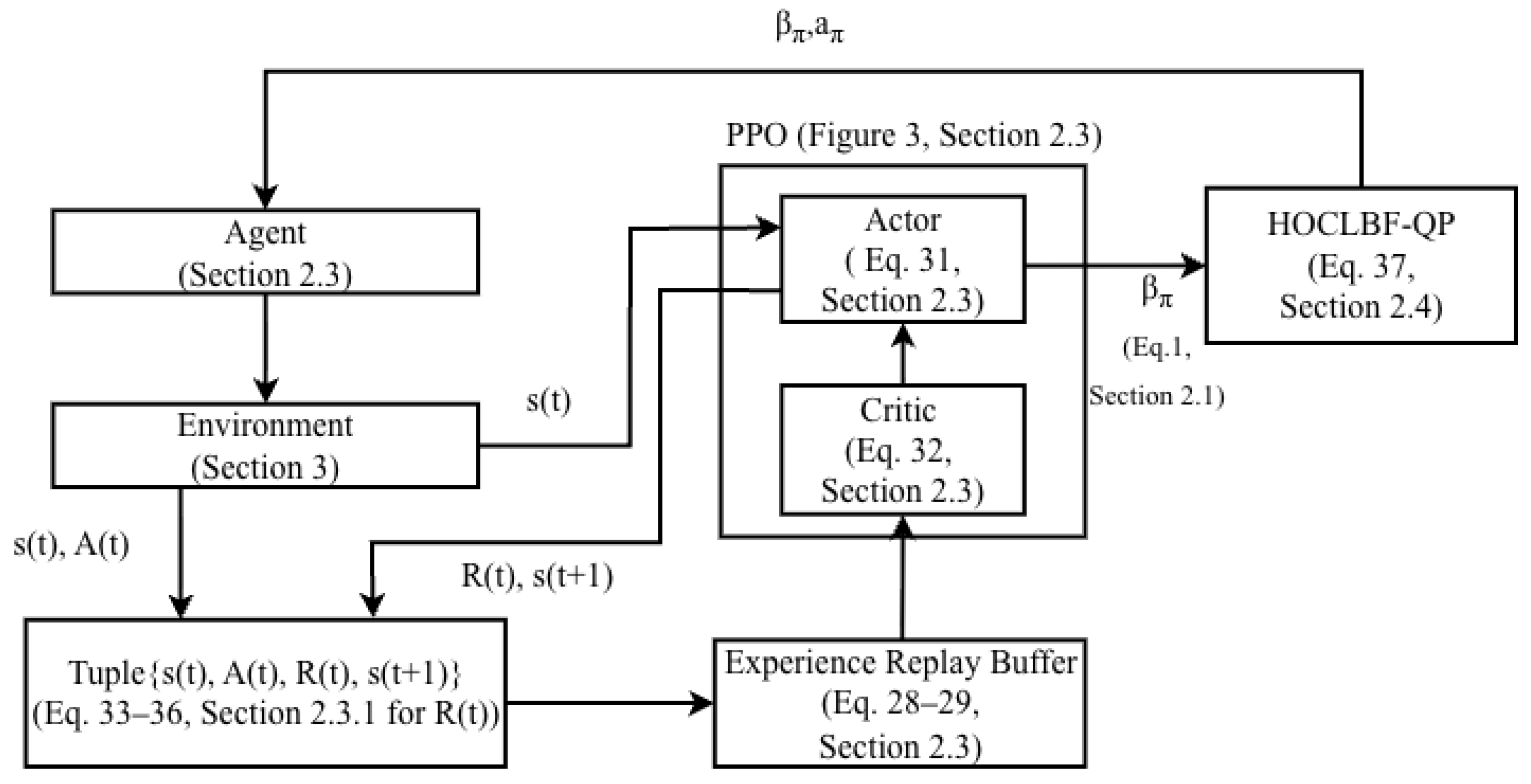
Furthermore, the modeling assumptions made for the sake of tractability impose constraints on the range of situations in which the current guarantees remain valid. The vehicle is represented by a kinematic bicycle model that intentionally omits various factors, including inertial forces, mass distribution, and tire slip dynamics. A small slip angle linearization ( cos β = 1 , sin β = β ) is employed to derive the control-affine form used in both the CLF-CBF constraints and the HOCLBF-QP filter. While these simplifications are justified for the moderate speeds addressed in this study, specifically with the agent operating at a maximum longitudinal velocity of 1.0 m / s , they become increasingly invalid in scenarios involving aggressive cornering, high-speed lane changes, or surfaces with limited friction, where lateral dynamics and load transfer significantly influence behavior.
Moreover, the current benchmark focuses on a single occluded pedestrian crossing at controlled speeds, which is sufficient for studying the braking and recovery behavior central to this work. However, it does not encompass the full range of urban conditions. Furthermore, all results are obtained in the Webots simulator under idealized sensing and actuation; sensor noise, detection latency, actuator saturation, and the broader sim-to-real transfer gap are not yet assessed.
Finally, a related assumption concerns the pedestrian model. The second-order barrier (24) is derived under a locally constant pedestrian velocity ( v ˙ p , x = v ˙ p , y = 0 ), as explained following its definition in Section 2.2.2. If the pedestrian accelerates, the true second derivative of h differs from the modeled L f 2 h ( x ) by a term proportional to the unmodeled pedestrian acceleration, and the forward-invariance guarantee of Theorem 1—which presumes (24) is enforced exactly—no longer strictly holds over that interval. Because the filter re-solves (37) at every 40 ms control step using the freshly observed pedestrian velocity, the exposure window for this mismatch is bounded to a single control period rather than the full maneuver, which limits but does not eliminate the resulting risk. A formal robustness margin under bounded pedestrian acceleration—for example, an input-to-state-safe extension of the barrier condition—is a natural direction for future work.
These directions are directly related to the scenario generation and intent estimation work outlined in Section 6, which aims to provide the diverse and correlated traffic situations necessary for effective evaluation.
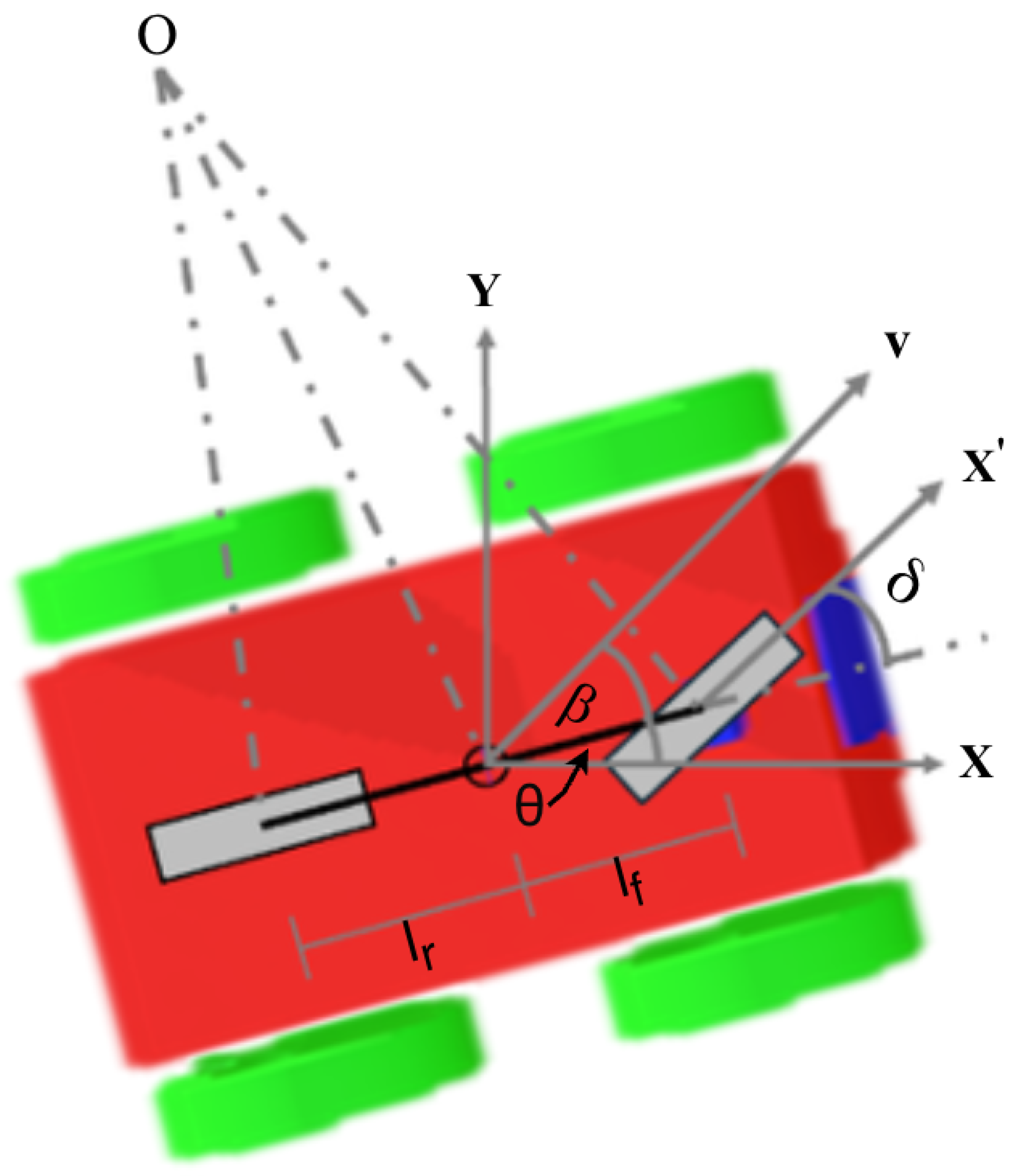
6. Conclusions

This paper presents a dual-layer framework aimed at enhancing the safety of autonomous vehicles in occluded urban driving scenarios, specifically focusing on pedestrian avoidance. The framework integrates a first-order Control Lyapunov–Barrier Function with Proximal Policy Optimization (CLBF-PPO) to regulate slip-angle control, alongside a Higher-Order Control Lyapunov–Barrier Function with Quadratic Programming (HOCLBF-QP) for real-time acceleration management.
The key innovation of this research lies in bridging the divide between learning-based adaptability and the rigorous stability and safety assurances provided by formal methods. This is achieved by allowing each method to operate within its domain of inherent strength. During the training phase, the analytical Lie derivatives of the Lyapunov and barrier functions are incorporated as modifiers within the PPO advantage estimate. This approach injects structural stability and safety signals into the training loop, enhancing the policy’s capability to achieve its goals while ensuring collision avoidance, without disrupting the standard updates of the PPO algorithm.
In the deployment phase, the HOCLBF-QP layer serves as a mathematically grounded safety filter. It adjusts the nominal acceleration of the vehicle to conform to the intersection of the higher-order Lyapunov and barrier feasibility sets, extending the barrier formulation to include relative velocity terms to account for dynamic pedestrian movements. Consequently, the framework culminates in an integrated architecture where a learned policy and an optimization-based safety mechanism are jointly designed within a unified Lyapunov–barrier formalism.
A simulation study conducted on a four-wheeled vehicle within the Webots environment corroborates the qualitative assertions of the proposed framework. The incorporation of the first-order CLBF advantage modifier infuses explicit stability and safety information into the policy gradient, resulting in accelerated and more stable convergence while generating trajectories that adhere to safety margins amidst both static and dynamic obstacles. Notably, the influence of each modifier weight is non-monotonic; a moderate weighting enriches the learning signal, whereas excessive weighting can destabilize training or lead to overly conservative policies that prioritize safety at the expense of efficient goal attainment. In addition, the HOCLBF-QP layer orchestrates the temporal dynamics of braking and goal-recovery maneuvers, with the higher-order Lyapunov and barrier coefficients jointly determining the agent’s responsiveness to imminent hazards while modulating speed in accordance with the remaining safety margin.
Through various pedestrian crossing scenarios of differing complexities, the integrated controller consistently demonstrates a coherent sequence of braking and recovery that maintains the forward invariance of the barrier safety set, while restoring convergence to the goal once the hazard has been cleared. This behavior is not replicable by a traditional HOCLBF-QP baseline, which lacks a goal-consistent learned policy. These findings collectively affirm that the synergistic interaction of the two layers—rather than their isolated implementation—is pivotal for enabling safe and purposeful navigation in emergency situations.
The broader implications of this work suggest that safety-critical learning-based control systems significantly benefit from being developed within, rather than merely layered over, a Lyapunov–barrier formalism. By embedding stability and safety criteria directly into the learning signals, the alignment of the policy’s inductive bias with the geometric structure enforced by the deployment-time safety filter is achieved. This results in a controller that is adaptive to perceptual and environmental uncertainties while ensuring instantaneous safety and long-term stability. Nonetheless, the present framework is limited by its dependence on manually tuned weights and class- K coefficients, as well as the simplifying assumptions inherent in the kinematic bicycle model with small-slip-angle linearization, alongside a benchmark restricted to a single occluding obstacle and a solitary observable pedestrian.
Future research will focus on four main directions, each addressing a limitation identified in Section 5.
First, to eliminate the reliance on manually tuned weights and class- K coefficients, we will explore adaptive and self-supervised mechanisms. These include meta-learned or Bayesian-optimized schedules, as well as differentiable tuning of coefficients through the QP layer. This approach will allow us to recalibrate d l , d s , d p , and α l , 1 , α l , 2 , α p , 1 , α p , 2 in real time, responding to variations in pedestrian speed, road geometry, and vehicle dynamics. Second, to extend the applicability beyond low-speed scenarios, we will replace the kinematic bicycle model with a more accurate dynamic bicycle or full-vehicle model. This new model will account for tire forces, load transfer, and yaw dynamics. Additionally, we will provide a formal characterization of the QP feasibility region under these more complex dynamics. Furthermore, A broader statistical validation over a larger number of random seeds, enabling confidence-interval estimation across all configurations, is also planned to complement the dispersion analysis reported here.
Third, we will generalize the higher-order barrier formulation from a single, fully observable pedestrian to a setting with dense, partially observable, multi-pedestrian environments. This involves coupling the safety filter with probabilistic intent estimation, so that the closing-rate term reflects predicted pedestrian motion rather than just instantaneous motion. As part of this direction, we will also establish a formal robustness margin under bounded pedestrian acceleration—for example, an input-to-state-safe extension of the barrier condition—so that the forward-invariance guarantee degrades gracefully when the constant-velocity assumption of the present filter is violated. Fourth, an important complementary direction is the systematic generation of complex traffic scenarios for training and stress testing. Spatiotemporal graph generative models, which represent multiple interacting agents as a time-varying graph, have shown promise in other fields, such as power system generation [48,49], for handling spatiotemporally correlated uncertainty. Furthermore, experiments on hardware-in-the-loop testing and real-vehicle validation will be a part of our future work. To enhance our research, we will implement scenario-clustering techniques to identify and prioritize safety-critical situations. This approach will provide a significantly more robust benchmark than the fixed-trajectory pedestrian scenarios discussed in this paper. Additionally, the distributions of the generated scenarios can serve to inform the probabilistic intent estimates that are vital for establishing effective barrier constraints.
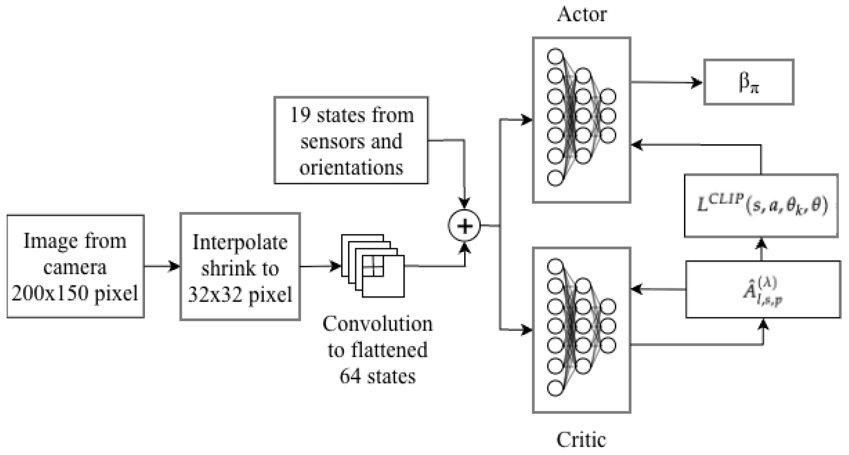
By pursuing these research directions, we aim to strengthen the role of unified, learning-based, mathematically grounded controllers as a foundational framework for the safe deployment of autonomous vehicles in real-world urban traffic environments.

Author Contributions

Conceptualization, C.-K.P. and T.C.; methodology, T.C.; software, T.C.; validation, C.-K.P. and T.C.; formal analysis, T.C.; investigation, T.C.; resources, T.C.; data curation, T.C.; writing—original draft preparation, T.C.; writing—review and editing, C.-K.P. and T.C.; visualization, T.C.; supervision, C.-K.P.; project administration, C.-K.P. All authors have read and agreed to the published version of the manuscript.

Funding

This research received no external funding.

Institutional Review Board Statement

Not applicable.

Informed Consent Statement

Not applicable.

Data Availability Statement

The numerical data that underpins the findings of this study, including detailed per-run logs that contribute to the figures and tables, are available for your review. For any further inquiries, we encourage you to contact the corresponding author for assistance.

Acknowledgments

The author would like to express his gratitude to the Royal Thai Government Scholarship (Ministry of Higher Education, Science, Research and Innovation) for receiving the Scholarship during his Ph.D. program, alleviating financial burdens and enabling him to focus wholeheartedly on his research.

Conflicts of Interest

The authors declare no conflicts of interest.

Appendix A

Table A1. Hyperparameters in the CLBF-PPO experiment.
DescriptionValue
Actor Learning Rate ( α θ )3 × 10⁻⁵
Critic Learning Rate ( α θ ^ )3 × 10⁻⁵
Discount Rate ( γ )0.99
GAE decay coefficient ( λ )0.95
Entropy Coefficient ( φ )0.05
Experience Replay Pool1024
Experience Replay Batch256
Epoch10
Exploration Episode3000

References

  1. World Health Organization (WHO). Global Status Report on Road Safety 2023; World Health Organization: Geneva, Switzerland, 2023. [Google Scholar]
  2. Blincoe, L.; Miller, T.; Wang, J.S.; Swedler, D.; Coughlin, T.; Lawrence, B.; Guo, F.; Klauer, S.; Dingus, T. The Economic and Societal Impact of Motor Vehicle Crashes, 2019 (Revised); Report DOT HS 813 403; National Highway Traffic Safety Administration: Washington, DC, USA, 2023.
  3. Nageshrao, S.; Tseng, H.E.; Filev, D. Autonomous Highway Driving using Deep Reinforcement Learning. In Proceedings of the 2019 IEEE International Conference on Systems, Man and Cybernetics (SMC), Bari, Italy, 6–9 October 2019; IEEE: New York, NY, USA, 2019; pp. 2326–2331. [Google Scholar] [CrossRef]
  4. Martínez-Díaz, M.; Soriguera, F. Autonomous vehicles: Theoretical and practical challenges. Transp. Res. Procedia 2018, 33, 275–282. [Google Scholar] [CrossRef]
  5. Aleksa, M.; Schaub, A.; Erdelean, I.; Wittmann, S.; Soteropoulos, A.; Fürdös, A. Impact Analysis of Advanced Driver Assistance Systems (ADAS) Regarding Road Safety–Computing Reduction Potentials. Eur. Transp. Res. Rev. 2024, 16, 39. [Google Scholar] [CrossRef]
  6. Terapaptommakol, W.; Phaoharuhansa, D.; Koowattanasuchat, P.; Rajruangrabin, J. Design of Obstacle Avoidance for Autonomous Vehicle Using Deep Q-Network and CARLA Simulator. World Electr. Veh. J. 2022, 13, 239. [Google Scholar] [CrossRef]
  7. Fu, H.; Wang, Q.; He, H. Path-Following Navigation in Crowds with Deep Reinforcement Learning. IEEE Internet Things J. 2024, 11, 20236–20245. [Google Scholar] [CrossRef]
  8. Li, J.; Tang, C.; Tomizuka, M.; Zhan, W. Hierarchical Planning Through Goal-Conditioned Offline Reinforcement Learning. IEEE Robot. Autom. Lett. 2022, 7, 10216–10223. [Google Scholar] [CrossRef]
  9. Chen, H.; Cao, X.; Guvenc, L.; Aksun-Guvenc, B. Deep-Reinforcement-Learning-Based Collision Avoidance of Autonomous Driving System for Vulnerable Road User Safety. Electronics 2024, 13, 1952. [Google Scholar] [CrossRef]
  10. Chen, Y.; Lam, C.T.; Pau, G.; Ke, W. From Virtual to Reality: A Deep Reinforcement Learning Solution to Implement Autonomous Driving with 3D-LiDAR. Appl. Sci. 2025, 15, 1423. [Google Scholar] [CrossRef]
  11. Li, D.; Okhrin, O. A Platform-Agnostic Deep Reinforcement Learning Framework for Effective Sim2Real Transfer Towards Autonomous Driving. Commun. Eng. 2024, 3, 147. [Google Scholar] [CrossRef] [PubMed]
  12. Raj, R.; Kos, A. Intelligent Mobile Robot Navigation in Unknown and Complex Environment Using Reinforcement Learning Technique. Sci. Rep. 2024, 14, 22852. [Google Scholar] [CrossRef] [PubMed]
  13. Wu, Z.; Albalawi, F.; Zhang, Z.; Zhang, J.; Durand, H.; Christofides, P.D. Control Lyapunov-Barrier Function-Based Model Predictive Control of Nonlinear Systems. In Proceedings of the 2018 Annual American Control Conference (ACC), Milwaukee, WI, USA, 27–29 June 2018; IEEE: New York, NY, USA, 2018; pp. 5920–5926. [Google Scholar] [CrossRef]
  14. Ding, Y.; Zhong, H.; Qian, Y.; Wang, L.; Xie, Y. Lane-Change Collision Avoidance Control for Automated Vehicles with Control Barrier Functions. Int. J. Automot. Technol. 2023, 24, 739–748. [Google Scholar] [CrossRef]
  15. He, S.; Zeng, J.; Zhang, B.; Sreenath, K. Rule-Based Safety-Critical Control Design using Control Barrier Functions with Application to Autonomous Lane Change. In Proceedings of the 2021 American Control Conference (ACC), New Orleans, LA, USA, 25–28 May 2021; IEEE: New York, NY, USA, 2021; pp. 178–185. [Google Scholar] [CrossRef]
  16. Hamdada, O.; Kribeche, A.; Chaibet, A.; Andrianarison, O. Optimizing Autonomous Vehicle Control and Safety with the CLF-CBF-QP Framework for Dynamic Driving Scenarios. In Proceedings of the 2025 International Conference on Control, Automation and Diagnosis (ICCAD), Barcelona, Spain, 1–3 July 2025; IEEE: Nevers, France, 2025; pp. 1–7. [Google Scholar] [CrossRef]
  17. Silva, D.; Silvestre, D. Guaranteed collision avoidance for autonomous surface vehicles equipped with a LiDAR using a CLF-CBF-QP controller. Eur. J. Control 2025, 86, 101377. [Google Scholar] [CrossRef]
  18. Wang, L.; Ames, A.D.; Egerstedt, M. Safety Barrier Certificates for Collisions-Free Multirobot Systems. IEEE Trans. Robot. 2017, 33, 661–674. [Google Scholar] [CrossRef]
  19. Allamaa, J.P.; Patrinos, P.; Ohtsuka, T.; Son, T.D. Real-time MPC with Control Barrier Functions for Autonomous Driving using Safety Enhanced Collocation. IFAC-PapersOnLine 2024, 58, 392–399. [Google Scholar] [CrossRef]
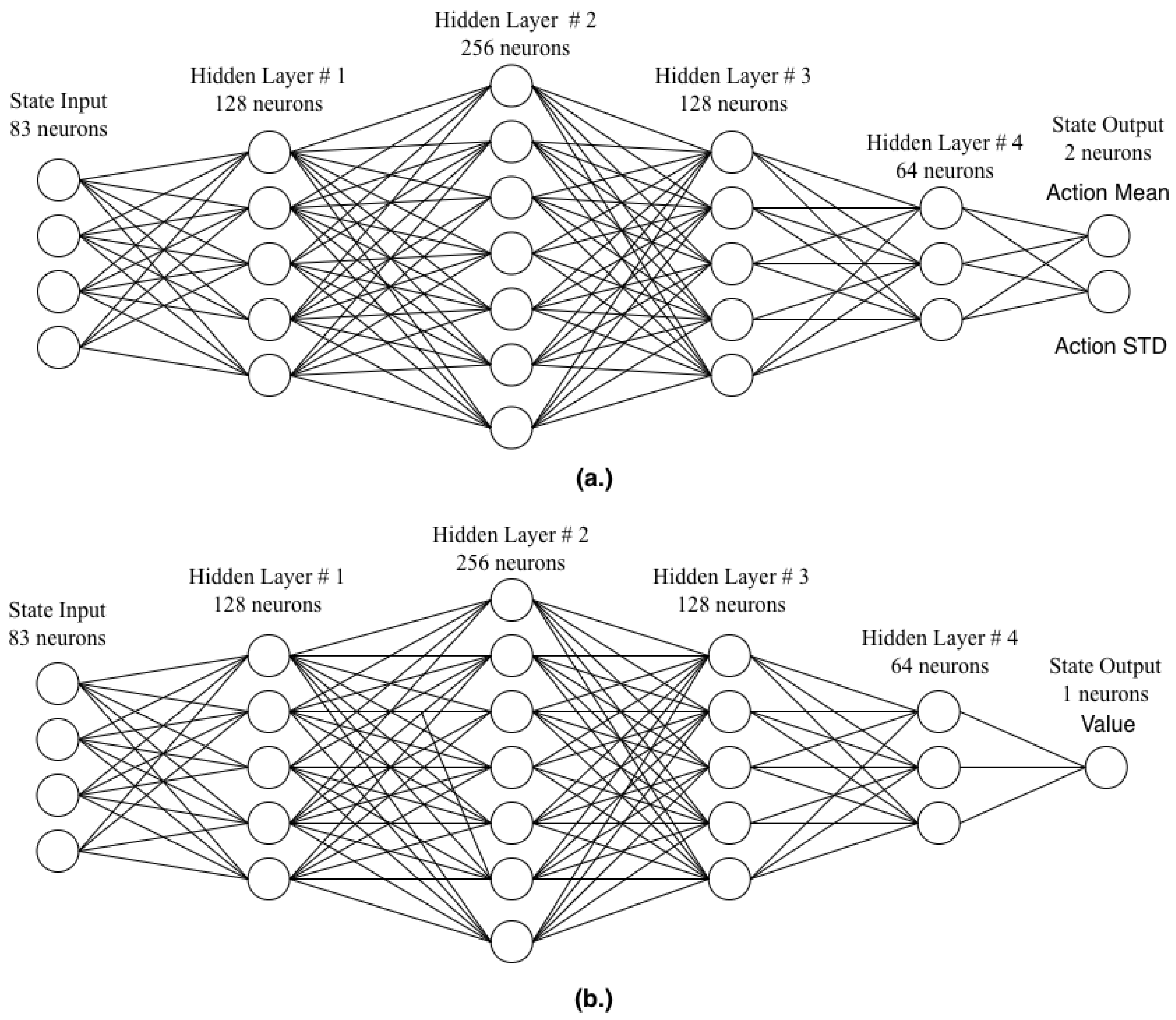
  20. Cohen, M.H.; Belta, C. Safe Exploration in Model-Based Reinforcement Learning Using Control Barrier Functions. arXiv 2021, arXiv:2104.08171. [Google Scholar]
  21. Cheng, R.; Orosz, G.; Murray, R.M.; Burdick, J.W. End-to-End Safe Reinforcement Learning through Barrier Functions for Safety-Critical Continuous Control Tasks. In Proceedings of the AAAI Conference on Artificial Intelligence, Honolulu, HI, USA, 27 January–1 February 2019; The Association for the Advancement of Artificial Intelligence: Washington, DC, USA, 2019; Volume 33, pp. 3387–3395. [Google Scholar] [CrossRef]
  22. Zhang, Y.; Liang, X.; Li, D.; Ge, S.S.; Gao, B.; Chen, H.; Lee, T.H. Barrier Lyapunov Function-Based Safe Reinforcement Learning for Autonomous Vehicles with Optimized Backstepping. IEEE Trans. Neural Netw. Learn. Syst. 2024, 35, 2066–2080. [Google Scholar] [CrossRef] [PubMed]
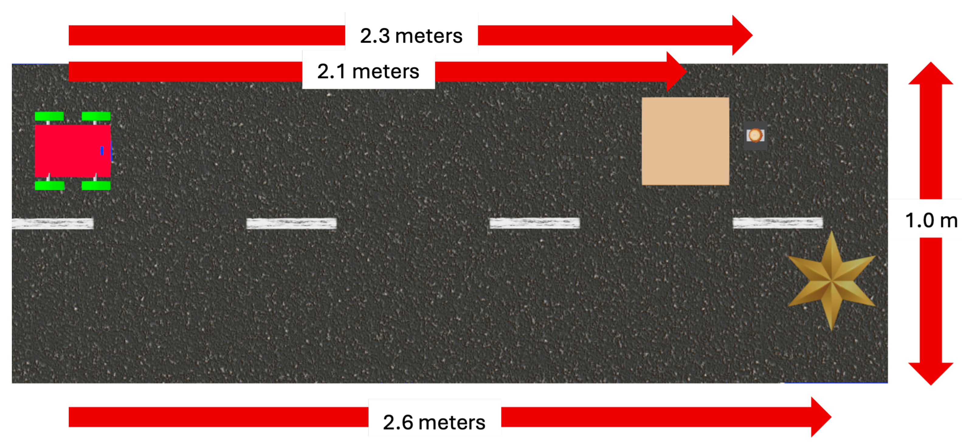
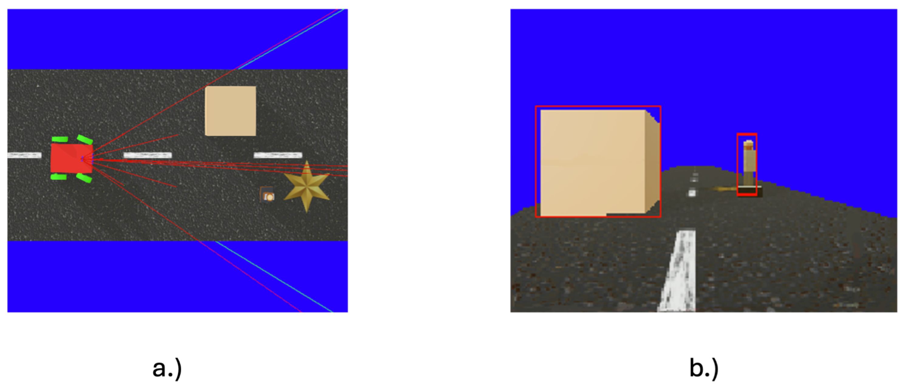
  23. Wang, P.; Liang, X.; Peng, X.; Lu, Y.; Ge, S.S. Control Barrier Performance Function-Based Cooperative Formation with Parallel Dynamic Event-Triggering Strategy. IEEE Trans. Syst. Man Cybern. Syst. 2024, 54, 4552–4564. [Google Scholar] [CrossRef]
  24. Ma, H.; Chen, J.; Li, S.E.; Lin, Z.; Guan, Y.; Ren, Y.; Zheng, S. Model-Based Constrained Reinforcement Learning Using Generalized Control Barrier Function. In Proceedings of the 2021 IEEE/RSJ International Conference on Intelligent Robots and Systems (IROS), Prague, Czech Republic, 27 September–1 October 2021; IEEE: New York, NY, USA, 2021; pp. 4552–4559. [Google Scholar] [CrossRef]
  25. Chen, H.; Zhang, F.; Aksun-Guvenc, B. Collision Avoidance in Autonomous Vehicles Using the Control Lyapunov Function–Control Barrier Function–Quadratic Programming Approach with Deep Reinforcement Learning Decision-Making. Electronics 2025, 14, 557. [Google Scholar] [CrossRef]
  26. Chen, H.; Aksun-Guvenc, B. Hierarchical Deep Reinforcement Learning-Based Path Planning with Underlying High-Order Control Lyapunov Function–Control Barrier Function–Quadratic Programming Collision Avoidance Path Tracking Control of Lane-Changing Maneuvers for Autonomous Vehicles. Electronics 2025, 14, 2776. [Google Scholar] [CrossRef]
  27. Polack, P.; Altché, F.; d’Andréa Novel, B.; de La Fortelle, A. The kinematic bicycle model: A consistent model for planning feasible trajectories for autonomous vehicles? In Proceedings of the 2017 IEEE Intelligent Vehicles Symposium (IV), Los Angeles, CA, USA, 11–14 June 2017; IEEE: New York, NY, USA, 2017; pp. 812–818. [Google Scholar] [CrossRef]
  28. Hu, X.; Wang, P.; Cai, S.; Zhang, L.; Hu, Y.; Chen, H. Vehicle Stability Analysis by Zero Dynamics to Improve Control Performance. IEEE Trans. Control Syst. Technol. 2023, 31, 2365–2379. [Google Scholar] [CrossRef]
  29. Shevitz, D.; Paden, B. Lyapunov stability theory of nonsmooth systems. IEEE Trans. Autom. Control 1994, 39, 1910–1914. [Google Scholar] [CrossRef]
  30. Li, B.; Wen, S.; Yan, Z.; Wen, G.; Huang, T. A Survey on the Control Lyapunov Function and Control Barrier Function for Nonlinear-Affine Control Systems. IEEE/CAA J. Autom. Sin. 2023, 10, 584–602. [Google Scholar] [CrossRef]
  31. Kushwaha, D.S.; Biron, Z.A. A Review on Safe Reinforcement Learning Using Lyapunov and Barrier Functions. arXiv 2026, arXiv:2508.09128. [Google Scholar]
  32. Chen, H.; Cao, X.; Guvenc, L.; Aksun-Guvenc, B. High Order Control Lyapunov Function-Control Barrier Function-Quadratic Programming Based Autonomous Driving Controller for Bicyclist Safety. arXiv 2025, arXiv:2512.12776. [Google Scholar]
  33. Xiao, W.; Belta, C.A.; Cassandras, C.G. High Order Control Lyapunov-Barrier Functions for Temporal Logic Specifications. In Proceedings of the 2021 American Control Conference (ACC), New Orleans, LA, USA, 25–28 May 2021; IEEE: New York, NY, USA, 2021; pp. 4886–4891. [Google Scholar] [CrossRef]
  34. Gurriet, T.; Singletary, A.; Reher, J.; Ciarletta, L.; Feron, E.; Ames, A. Towards a Framework for Realizable Safety Critical Control through Active Set Invariance. In Proceedings of the 2018 ACM/IEEE 9th International Conference on Cyber-Physical Systems (ICCPS), Porto, Portugal, 11–13 April 2018; IEEE: New York, NY, USA, 2018; pp. 98–106. [Google Scholar] [CrossRef]
  35. Loshchilov, I.; Hutter, F. Decoupled Weight Decay Regularization. arXiv 2019, arXiv:1711.05101. [Google Scholar]
  36. Cocaul, P.; Bertrand, S.; Piet-Lahanier, H.; Lemazurier, L.; Ganet, M. Deep Reinforcement Learning design of safe, stable and robust control for sloshing-affected space launch vehicles. Control Eng. Pract. 2025, 161, 106328. [Google Scholar] [CrossRef]
  37. Shen, Y. Proximal Policy Optimization with Entropy Regularization. In Proceedings of the 2024 4th International Conference on Computer, Control and Robotics (ICCCR), Shanghai, China, 19–21 April 2024; IEEE: New York, NY, USA, 2024; pp. 380–383. [Google Scholar] [CrossRef]
  38. Serfilippi, L.; Franceschelli, G.; Corradi, A.; Musolesi, M. Complexity-Regularized Proximal Policy Optimization. arXiv 2026, arXiv:2509.20509. [Google Scholar]
  39. Ma, S.; Li, D.; Hu, T.; Xing, Y.; Yang, Z.; Nai, W. Huber Loss Function Based on Variable Step Beetle Antennae Search Algorithm with Gaussian Direction. In Proceedings of the 2020 12th International Conference on Intelligent Human-Machine Systems and Cybernetics (IHMSC), Hangzhou, China, 22–23 August 2020; IEEE: New York, NY, USA, 2020; Volume 1, pp. 248–251. [Google Scholar] [CrossRef]
  40. Cheng, C.H.; Lin, H.H.; Luo, Y.Y. Research on Autonomous Vehicle Lane-Keeping and Navigation System Based on Deep Reinforcement Learning: From Simulation to Real-World Application. Electronics 2025, 14, 2738. [Google Scholar] [CrossRef]
  41. Stellato, B.; Banjac, G.; Goulart, P.; Bemporad, A.; Boyd, S. OSQP: An operator splitting solver for quadratic programs. Math. Program. Comput. 2020, 12, 637–672. [Google Scholar] [CrossRef]
  42. Xiao, W.; Belta, C. High-Order Control Barrier Functions. IEEE Trans. Autom. Control 2022, 67, 3655–3662. [Google Scholar] [CrossRef]
  43. Michel, O. Cyberbotics Ltd. Webots™: Professional Mobile Robot Simulation. Int. J. Adv. Robot. Syst. 2004, 1, 39–42. [Google Scholar] [CrossRef] [PubMed]
  44. Kirtas, M.; Tsampazis, K.; Passalis, N.; Tefas, A. Deepbots: A Webots-Based Deep Reinforcement Learning Framework for Robotics. In Proceedings of the Artificial Intelligence Applications and Innovations; Maglogiannis, I., Iliadis, L., Pimenidis, E., Eds.; Springer: Cham, Switzerland, 2020; pp. 64–75. [Google Scholar]
  45. Trararak, C.; Hoang, T.T.; Cong-Kha, P. Pedestrian Avoidance Simulation by Deep Reinforcement Learning Using Webots. In Proceedings of the 2025 International Conference on Artificial Intelligence in Information and Communication (ICAIIC), Fukuoka, Japan, 18–21 February 2025; IEEE: New York, NY, USA, 2025; pp. 0734–0739. [Google Scholar] [CrossRef]
  46. Luo, W.; Wang, X.; Han, F.; Zhou, Z.; Cai, J.; Zeng, L.; Chen, H.; Chen, J.; Zhou, X. Research on LSTM-PPO Obstacle Avoidance Algorithm and Training Environment for Unmanned Surface Vehicles. J. Mar. Sci. Eng. 2025, 13, 479. [Google Scholar] [CrossRef]
  47. Reghenzani, F.; Massari, G.; Fornaciari, W. The Real-Time Linux Kernel: A Survey on PREEMPT_RT. ACM Comput. Surv. 2019, 52, 1–36. [Google Scholar] [CrossRef]
  48. Hu, J.; Cao, Y.; Tan, G. A dynamic spatiotemporal graph generative adversarial network for scenario generation of renewable energy with nonlinear dependence. Energy 2025, 335, 138049. [Google Scholar] [CrossRef]
  49. Hu, J.; Liu, Y.; Chai, Y.; Tan, G. An adaptive dynamic scenario clustering method for power system optimization control under spatiotemporal correlated uncertainties. Meas. Sci. Technol. 2026, 37, 236206. [Google Scholar] [CrossRef]
Figure 1. Integration of CLBF-PPO and HOCLBF-QP optimization algorithm for pedestrian avoidance.
Electronics 15 03026 g001
Figure 2. Kinematics Bicycle Vehicle Dynamics.
Electronics 15 03026 g002
Figure 3. Overview of the CLBF-PPO algorithm.
Electronics 15 03026 g003
Figure 4. PPO network structure (a.) actor network; (b.) critic network.
Electronics 15 03026 g004
Figure 5. Pedestrian-avoidance scenario simulated on Webots simulator.
Electronics 15 03026 g005
Figure 6. Camera perception in the vehicle. (a.) the camera’s field of view (b.) the camera perception using recognition features.
Electronics 15 03026 g006
Figure 7. Robot-supervisor scheme on deepbots [45].
Electronics 15 03026 g007
Figure 8. Reward comparison under varying control Lyapunov weight d l .
Electronics 15 03026 g008
Figure 9. Reward comparison under control Lyapunov weight d l = 0.10 , against baseline PPO and PPO-LSTM (50-episode moving average).
Electronics 15 03026 g009
Figure 10. Agent’s trajectories on control Lyapunov weight over PPO(MLP) and PPO-LSTM.
Electronics 15 03026 g010
Figure 11. Reward comparison under varying control barrier weight on static obstacle(the box) d s , on the fixed control Lyapunov weight d l = 0.10 .
Electronics 15 03026 g011
Figure 12. Agent’s trajectories under varying control barrier weight on static obstacle (the box) d s .
Electronics 15 03026 g012
Figure 13. Reward comparison under varying control barrier weight on pedestrian d p , on the fixed control Lyapunov weight d l = 0.10 and d s = 0.05 .
Electronics 15 03026 g013
Figure 14. Agent’s trajectories under varying control barrier weight on pedestrian d p .
Electronics 15 03026 g014
Figure 15. Agent’s velocity and acceleration over various α p , 2 on the fix of α p , 1 = 1.00.
Electronics 15 03026 g015
Figure 16. Agent’s trajectories on the change of α p , 2 .
Electronics 15 03026 g016
Figure 17. Agent’s velocity and acceleration over various α p , 1 on the fix of α p , 2 = 1.00.
Electronics 15 03026 g017
Figure 18. Agent’s trajectories on the change of α p , 1 .
Electronics 15 03026 g018
Figure 19. Agent’s velocity and acceleration over various α l , 2 on the fix of α l , 1 = 1.00.
Electronics 15 03026 g019
Figure 20. Agent’s trajectories on the change of α l , 2 .
Electronics 15 03026 g020
Figure 21. Agent’s velocity and acceleration over various α l , 1 on the fix of α l , 2 = 1.00.
Electronics 15 03026 g021
Figure 22. Agent’s trajectories on the change of α l , 1 .
Electronics 15 03026 g022
Figure 23. The characteristics of agent’s driving behavior in a pedestrian speed at 0.325 m / s between CLBF-PPO-HOCLBF-QP and traditional HOCLBF-QP (a) the agent’s trajectory (b) the agent’s velocity (c) the agent’s acceleration (d) the agent’s steering angle.
Electronics 15 03026 g023
Figure 24. The characteristics of agent’s driving behavior in a pedestrian speed at 0.425 m / s between CLBF-PPO-HOCLBF-QP and traditional HOCLBF-QP (a) the agent’s trajectory (b) the agent’s velocity (c) the agent’s acceleration (d) the agent’s steering angle.
Electronics 15 03026 g024
Figure 25. The characteristics of agent’s driving behavior in a pedestrian speed at 0.500 m / s between CLBF-PPO-HOCLBF-QP and traditional HOCLBF-QP (a) the agent’s trajectory (b) the agent’s velocity (c) the agent’s acceleration (d) the agent’s steering angle.
Electronics 15 03026 g025
Figure 26. Computational time of the quadratic programming time (QP) solver in Equation (37) and total time step.
Electronics 15 03026 g026
Table 1. Positioning of the proposed framework against the closest control-, hierarchical-, and learning-based safety approaches.
MethodLearning ObjectiveSafety FilterObstacle TypeRelative-Degree TreatmentDynamic-Obstacle ModelingValidation Environment
Proposed (this work)Continuous slip-angle policy (PPO) with a CLBF-modified advantageHOCLBF–QP at deployment, co-designed with the policy on shared certificatesStatic obstacle and an occluded crossing pedestrianFirst-order CLF/CBF in the training advantage; second-order (HOCLBF) in the deployment QPRelative velocity (closing-rate) barrier termWebots four-wheeled vehicle, real time at 25 Hz
CLF-CBF-QP control [16,17]None; hand-designed nominal/reference inputCLF–CBF–QPStatic and moving obstaclesFirst-orderPosition-based CBFSimulink and surface-vehicle experiment
DRL decision + CLF-CBF-QP [25]Discrete high-level decision (DRL), trained separately from the filterCLF–CBF–QP low-level, independently designedStatic and dynamic obstacle setupsFirst-orderPosition-based CBFSimulink MIL and real-time, unicycle model
DDQN decision + HOCLF-HOCBF-QP [26]Discrete lane-maneuver selection (DDQN), trained separately from the filterHOCLF–HOCBF–QP low-level, independently designedLane change past a static/parked obstacleHigher-orderPosition-based path trackingSimulation, single-track lateral model
Safe RL with (generalized) CBF [20,21,24]Constrained policy optimization; barrier folded into trainingCBF/GCBF constraint inside the policy update; no deployment-time QPCollision-avoidance and safe-exploration tasksFirst-order [20,21]; higher-order via GCBF [24]Distance-to-boundary (position-based)Benchmark simulation in real vehicle
Table 2. Comparison on experiment results across control Lyapunov weights d l , against PPO and PPO-LSTM baselines.
AlgorithmAverage ReturnSuccess RateAverage Advantage
Baseline PPO 581.10 ± 202.52 28.00 % ± 45.00 % 155.80 ± 45.79
PPO-LSTM [46] 759.35 ± 178.53 47.43 % ± 49.94 % 163.00 ± 38.59
d l = 0.05 976.02 ± 145.52 88.13 % ± 32.34 % 171.72 ± 11.55
d l = 0.10 999.78 ± 104.56 90.40 % ± 29.46 % 199.75 ± 21.04
d l = 0.15 624.54 ± 225.02 37.20 % ± 48.34 % 142.81 ± 33.86
Table 3. Comparison on experiment results across control barrier weight on static obstacle d s , on the fixed control Lyapunov weight d l = 0.10 .
AlgorithmAverage ReturnSuccess RateAverage Advantage
d s = 0.00 999.76 ± 104.50 90.40 % ± 29.46 % 199.75 ± 21.04
d s = 0.05 1007.36 ± 95.74 95.83 % ± 19.98 % 192.52 ± 17.49
d s = 0.10 903.47 ± 164.15 80.27 % ± 39.81 % 170.43 ± 19.20
d s = 0.15 883.08 ± 141.98 77.67 % ± 41.65 % 158.77 ± 17.69
Table 4. Comparison on experiment results across control barrier weight on pedestrian d p , on the fixed d l = 0.10 and d s = 0.05 .
AlgorithmAverage ReturnSuccess RateAverage Advantage
d p = 0.00 817.84 ± 135.08 49.80 % ± 50.01 % 162.17 ± 24.65
d p = 0.05 824.54 ± 229.77 73.83 % ± 42.81 % 163.65 ± 17.02
d p = 0.10 884.29 ± 165.03 78.07 % ± 41.39 % 158.81 ± 15.09
d p = 0.15 658.51 ± 171.10 30.47 % ± 46.03 % 116.13 ± 18.54
Table 5. Quantitative comparison of the proposed CLBF-PPO-HOCLBF-QP framework and the traditional HOCLBF-QP baseline across the three pedestrian crossing speeds.
v p = 0.325  m/s v p = 0.425  m/s v p = 0.500  m/s
MetricProp.Trad.Prop.Trad.Prop.Trad.
Safety & Avoidance Response
   Min. ped. clearance (m)0.200.310.150.210.160.64
   Min. speed (m/s)0.691.000.001.000.001.00
   Peak decel. (m/s2) 0.42 0.00 0.63 0.00 0.63 0.00
   max δ (deg-turn right)10.9726.6513.5426.3713.530.00
   min δ (deg-turn left)−36.28−38.00−39.09−38.00−39.09−38.00
Goal Convergence
   Goal reachedYesYesYesYesYesNo
   Travel distance (m)2.742.782.752.782.752.23
   Completion time (s)2.722.764.722.804.72
Kinematic-Model Validity
   Max. slip angle | β | (deg)20.1521.3322.1121.3322.1121.33
   Max. lateral accel. | a y | (m/s2)4.314.554.314.554.314.55
   Max. curvature demand | κ | (m−1)4.314.554.714.554.714.55
   Max. friction util. ρ 0.520.550.520.550.520.55
QP Constraint Relaxation
   Barrier slack δ p (min) 0.00 0.00 0.00 0.00 0.00 0.00
   Barrier slack δ p (max) 0.00 0.00 0.00 0.00 0.00 0.00
   Stability slack δ l (min)0.000.000.000.000.000.00
   Stability slack δ l (max)7.190.838.250.758.250.30
Disclaimer/Publisher’s Note: The statements, opinions and data contained in all publications are solely those of the individual author(s) and contributor(s) and not of MDPI and/or the editor(s). MDPI and/or the editor(s) disclaim responsibility for any injury to people or property resulting from any ideas, methods, instructions or products referred to in the content.