Article

Balancing Energy and Mission Time in UAV Site Servicing on Graph Maps Through Dynamic Battery-Threshold Double Deep Q-Learning

by
Gabriele Gemignani
1,2,* and
Lorenzo Pollini
1,*
1
Department of Information Engineering, University of Pisa, Largo Lucio Lazzarino 1, 56122 Pisa, Italy
2
DAuSy National PhD Programme, Polytechnic of Bari, Department of Electrical and Information Engineering, Via Re David 200, 70125 Bari, Italy
*
Authors to whom correspondence should be addressed.
Electronics 2026, 15(14), 2984; https://doi.org/10.3390/electronics15142984
Submission received: 29 May 2026 / Revised: 3 July 2026 / Accepted: 6 July 2026 / Published: 8 July 2026
(This article belongs to the Special Issue Machine Learning Applications in Unmanned Aerial Vehicles and Drones)

Abstract

Unmanned Aerial Vehicles (UAVs) increasingly operate in missions requiring the simultaneous satisfaction of multiple objectives: reaching task locations, performing the correct service, and preserving sufficient onboard energy for continuous operation. Mission efficiency depends not only on task completion but also on managing the trade-off between service duration and battery recharging. This work proposes a Double Deep Q-Network (DDQN) policy for energy-aware UAV navigation on graph maps. The UAV must first collect the appropriate servicing tool from a depot node and then deliver it to the active failure node. At the same time, it autonomously decides when to interrupt the mission for recharging so as to ensure sufficient battery reserve throughout continuous operations, while minimizing task-servicing duration. The key contribution is an energy-aware reward based on a Dynamic Battery Threshold (DBT) computed from graph shortest-path distances to the nearest charging station, enabling a topology-aware recharge policy that is safer yet less conservative than a per-map tuned safety margin. Extensive Monte Carlo tests on increasingly complex graphs show that the proposed policy achieves a 100% task completion rate with always sufficient final battery to reach a charging node from the task node, while degrading less with map complexity and exhibiting greater robustness to stochastic battery dynamics than a pseudo-optimal baseline.

1. Introduction

Unmanned Aerial Vehicles (UAVs) are increasingly deployed in missions where limited battery capacity constrains operational endurance. In these settings, mission planning must jointly optimize task completion and battery safety: the UAV must decide not only which tasks to service and in what order, but also when it is necessary to interrupt the mission to recharge to avoid depletion [1,2].
Among the most critical aspects of autonomous UAV operation is energy-awareness: this does not consist in finding an energy-optimized path to a goal, as studied in different UAV literature works [3,4], but rather the vehicle’s capability to continuously monitor its battery state and decide when to interrupt task execution and return to a recharge home. Indeed, recent work explicitly models the recharge decision as a first-class variable in the UAV policy, for example via Reinforcement Learning (RL) in coverage missions [5] or joint mission-and-charging planning [6], and even in simulation-based studies that distinguish “work” and “recharge” decisions in UAV behavior [7].
Energy-awareness is more than a safety constraint or a simple Return-to-Home (RTH) rule: it is a mission-level decision variable that directly affects performance. A conservative policy that recharges too often increases mission duration, while an aggressive one risks battery depletion. The challenge is to determine when recharging is truly necessary and when the UAV can safely continue its task. This trade-off is illustrated in Figure 1, where the same environment leads to opposite outcomes depending on task placement. The optimal policy must adapt to the environment topology and to the joint agent–task state, a requirement for long-term autonomy in persistent deployment scenarios.
From an engineering perspective, this naturally leads to a multi-objective combinatorial problem whose complexity grows with the state dimension and the map topology, and is, in general, NP-hard [8]. This motivates the search for efficient and practically feasible navigation policies capable of balancing mission performance with strict energy constraints.

1.1. Literature Review

Early approaches to energy-aware UAV mission planning relied on heuristic strategies such as nearest-neighbor routing, shortest-path navigation, and manually tuned recharge rules [9,10]. These methods are simple and computationally inexpensive, but they do not optimize a global mission objective, ignore the long-term consequences of local decisions, and are poorly scalable as the environment or task complexity increases.
To address these limitations, many works have formulated energy-constrained routing and scheduling as optimization problems, typically using Mixed-Integer Linear Programming (MILP) or related variants. These formulations jointly model task allocation, path selection, and recharge scheduling, sometimes including the placement of stationary charging stations [11,12,13] or the routing of UGVs acting as mobile chargers [14,15]. While principled and occasionally optimal, such methods are NP-hard and become computationally intractable for large graphs or online re-planning, even when combined with meta-heuristic scheduling policies [16].
Learning-based energy-aware task scheduling has therefore gained attention due to its scalability in large, complex UAV missions [17]. RL has been applied to battery-constrained UAV routing by incorporating the battery state into the agent’s observations and explicitly modeling charging stations within the environment [18,19]. Fan et al. [20] formulate UAV traffic monitoring as a routing problem with multiple charging stations and, through a multi-head attention RL architecture, learn a policy that sequentially constructs the route optimizing energy consumption and path length minimization. Theile et al. [5] solve power-constrained coverage path planning with recharge actions using Proximal Policy Optimization (PPO). Ni et al. [21] tackle battery-limited coverage path planning with an Improved Double Deep Q-Network (IDDQN) that combined mechanisms like dynamic soft-update and Prioritized Experience Replay (PER) to improve sample efficiency under battery constraints. Chu et al. [22] study UAV data collection missions with joint speed control and energy replenishment, where RL optimizes both mobility and charging decisions. In multi-robot settings, RL has also been applied to cooperative UAV–UGV routing, where UGVs act as mobile charging stations and coordinated policies jointly optimize routing and recharging decisions [23]. For example, Mondal et al. [24,25], combine RL with expert-knowledge or attention-based architecture for cooperative route planning, overall showing improved mission efficiency and scalability in energy-constrained heterogeneous fleets.
The above RL approaches differ both in how they enforce energy-awareness (route-level versus per-step) and in how battery safety is designed. Route-construction methods typically optimize complete mission trajectories while accounting for battery feasibility and charging constraints [20,23,25,26]. Although battery state influences the generated routes, the required energy reserve is not explicitly formulated as a state-dependent function of the UAV position on the graph. Per-step RL are closer to our work, since recharge decisions are repeatedly taken during execution. However, they generally rely on manually tuned battery-related reward terms or fixed safety thresholds, like in [21] and our previous work [27]. These designs are inherently topology-agnostic: a threshold calibrated for a region densely served by charging stations is overly conservative there, yet unsafe in sparse regions far from any station, so it must be tuned for the worst-case configuration of the map, which extends mission time through unnecessary recharges. The closest formulation to ours is [22], where the reward combines residual energy with the Euclidean distance to a single charging station in a continuous environment. To the best of our knowledge, no RL formulations employ distance-based rewards that are explicitly defined from graph shortest-path distances to multiple charging stations.

1.2. Contributions and Paper Outline

In this work, we employ RL for solving an energy-aware site-servicing mission involving a UAV navigating on a graph map. In our case study, the UAV must collect the appropriate servicing tool from warehouse nodes, deliver it to active failure nodes, and autonomously plan intermediate recharges while minimizing the overall mission duration.
The main contributions of this paper are summarized as follows:
  • We propose a Double Deep Q-Network (DDQN) framework with a graph-aware Dynamic Battery-Threshold (DBT) reward based on Dijkstra shortest-path distances to the nearest recharge node. Unlike fixed battery safety margins, DBT defines a topology-aware energy reserve that adapts to heterogeneous graphs without per-map tuning, resulting, as proof of our experiments, in a more efficient trade-off between mission performance and battery safety. We adopt a value-based RL algorithm [28] rather than a policy-gradient one such as PPO, which has previously been shown to require ad hoc convergence tricks, like action masking and discount-factor scheduling, on comparable problems with large maps and sparse rewards [5].
  • We analyze the scalability of the proposed DDQN policy by increasing the graph dimension and the corresponding network size. To make policy training tractable as the state–action space grows with map complexity, we couple DDQN with PER, a combination already adopted for battery-constrained UAV path planning [21]. Across all benchmark graphs, the learned policy attains a 100% task completion rate with always enough final battery to at least reach a charging station after the successful fix. We further observe, in a continuous multi-task deployment where the agent’s battery is not reset from one test to another, a 0% discharge rate while minimizing mission length w.r.t. fixed-threshold policies, either too aggressive or conservative.
  • We compare the proposed DBT-DDQN policy against a model-based, pseudo-optimal planner. The results show that the RL policy achieves competitive mission efficiency, degrading less with increasing graph complexity and stochastic battery dynamics, all while maintaining significantly lower computational requirements.
The remainder of this paper is organized as follows. Section 2 introduces the graph-based mission formulation and the UAV and task model. Section 3 presents the proposed DDQN framework and the DBT reward shaping. Section 4 describes the simulation environment and the neural network implementation details. Section 5 reports the experimental results and comparative analyses. Finally, Section 6 discusses our findings and potential research directions.

2. Energy-Aware Site-Servicing on a Graph

Graph-based representations provide a compact and general abstraction for a broad class of autonomous mission planning problems. As illustrated in Figure 1, graph nodes can represent spatial waypoints in a physical environment, where the UAV navigates among task locations, charging stations, and transit points, but the same formulation applies equally to abstract task-transition structures or logistics networks, without loss of generality [29]. This section formalizes the graph environment and the site-servicing mission model and states the optimization problem that the proposed policy is designed to solve.

2.1. Graph and Mission Model

Consider a weighted undirected graph G = ( V , E , W ) , where V = { 1 , , N } is the set of N nodes, E V × V is the set of bidirectional edges, and  W : E R > 0 assigns a positive traversal cost to each edge. The graph is assumed connected, which is reasonable when building an ad hoc graph model for the environment at hand. The node set is partitioned into four subsets:
  • Target nodes V t V : Locations where failures occur and must be serviced.
  • Depot nodes V d V : Locations where the UAV collects servicing tools requested by targets. Tools can represent more general features that the UAV must possess in order to solve a specific requested task (e.g., a water tank in case of a wildfire, or package transportation, etc.).
  • Charging station nodes V c V : Locations where the UAV can recharge its battery, allowing uninterrupted autonomous operability. Recharge can occur autonomously via a landing policy on a charging platform or be conducted on-site by human operators.
  • Regular nodes V r = V ( V t V d V c ) : Transit nodes with no special mission function.
  • These subsets are not necessarily disjoint: a node v V d V c simultaneously offers tool pick-up and recharging capabilities. The only structural requirement is V t ( V d V c ) = , i.e., failures occur exclusively at non-service locations.
Let F = { 1 , , M } be the set of failure types, each requiring a dedicated tool. At any time, exactly one target node v V t is active with a failure of type f F . This single-failure assumption reflects a hierarchical decomposition of a multi-agent deployment: the proposed policy is the per-agent execution layer, while concurrency across tasks, priority scheduling, and task timeouts are handled by a higher-level task allocation algorithm that assigns at most one active failure per agent [30,31]. The UAV carries at most one tool at a time, encoded by τ T = { 0 } F , where τ = 0 denotes an empty payload.

2.2. Agent’s Energy Model

The onboard battery charge is described by a scalar b ( , 1 ] , where b = 1 denotes full charge and b 0 complete depletion. Note that the current model extends the battery to fictitious negative values for RL training, and that the goal of the policy will be, among others, to keep a positive level of battery throughout every mission request.
Denoting with a k the action selection at decision step k, the UAV selects one of four action types: move to an adjacent node, pick up a tool at a depot, fix the active failure, or recharge at a charging station. When a recharge action is executed at a charging node, the battery is instantly restored to full charge. This simple model assumes a UAV that enters a recharge mode and resumes the mission only once fully charged, overlooking the mission-time delay proportional to the time spent charging. For all other actions, the battery decreases by a stochastic amount depending on the action type:
Δ b k = clip N ( μ k , σ 2 ) , 0 , Δ b max ,
where σ > 0 is a noise, Δ b max > 0 is an upper bound on the per-step decay, and the deterministic mean μ k is proportional to the weight on the edge undergone if the UAV moved across adjacent graph edges, and it is constant otherwise, i.e.:
μ k = α W ( v k , a k ) if the UAV moves to an adjacent node , c 0 otherwise ,
with α > 0 a weight-to-consumption scaling factor and c 0 > 0 a fixed mean decay for non-movement operations. Real-world non-movement operations could, for instance, consist of hovering, asset control, or landing. Rather than adopting a detailed physical energy model as in existing works [3], the stochastic perturbation in (1) abstracts unmodeled low-level effects, such as imperfect trajectory tracking, wind disturbances, and uncertain payload dynamics. The energy-consumption model (1)–(2) is nevertheless modular: a higher-fidelity, physics-based consumption model can be substituted into the deterministic mean of the per-step decay in (2) without modifying the DBT reward or the DDQN policy, since the agent only observes the current battery state.

2.3. Problem Statement

The goal of the mission is to service the active failure in the minimum time. To ensure continuous operability beyond a single mission, the UAV must maintain a sufficient battery level throughout the episode, not only to avoid depletion during navigation, but also to guarantee that, upon completing the servicing task, enough charge remains to reach the nearest charging station. Denoting by π the UAV decision policy and by K the number of steps required to complete the mission, these requirements are captured by the following constrained minimization, where the expectation is taken over by the stochastic battery evolution:
min π E π [ K ] subject to b k b ̲ ( v k ) k < K ,
where b ̲ ( v k ) is a position-dependent battery safety margin ensuring sufficient residual charge to reach the nearest charging station from any node visited during the mission.
The problem is further subject to physical and model constraints: the UAV may only move along edges present in E , must perform a fix only at the active target v with the requested tool τ = f , and can only recharge and pick-up tools at the nodes v V c and v V d , respectively. Rather than enforcing these as hard constraints in (3), they are learned directly by the policy through the RL training process: infeasible actions are discouraged via dedicated penalty terms in the reward function, and the agent naturally internalizes admissibility as part of the learned value function, as detailed in Section 3.1.
The key challenge lies in the definition of b ̲ : how this margin is designed determines the trade-off between mission efficiency and energy safety, and is the subject of Section 3.2. The combinatorial structure, stochastic battery evolution, and the difficulty of calibrating this margin across heterogeneous map topologies make the problem intractable for exact methods at scale, motivating the learning-based approach presented next.

3. Reinforcement Learning Policy Design

The mission is cast as a Markov Decision Process (MDP) [32], and the optimal policy is approximated by a DDQN trained with our DBT reward contribution. The section is organized as follows: Section 3.1 defines the MDP state and action spaces; Section 3.2 reports the reward function with a focus on the relevance of the DBT term; Section 3.3 describes the training algorithm.

3.1. MDP Formulation

3.1.1. State Space

At each step k, the environment state is
s ¯ k = b k , v k , τ k , v , f ,
where b k is the battery level, v k V the current agent’s location, τ k T the onboard tool, and  v , f the active target and failure type, which remain unchanged until the fix action is successfully executed and the mission terminates.
At the beginning of each episode, the initial state s ¯ 0 is drawn according to
v 0 U ( V ) , τ 0 U ( T ) , b 0 U ( ( 0 , 1 ) ) , v U ( V t ) , f U ( F ) ,
where U ( · ) denotes a uniform distribution over the respective set or interval. Randomizing all state components at initialization promotes generalization of the learned policy across diverse mission configurations.
In our RL implementation, the battery level is encoded as a continuous scalar, while all the remaining discrete state components use a compact binary representation bin ( · ) , so that all inputs are normalized in the [ 0 , 1 ] range. The binary state vector provided to the neural network is therefore
s k = b k , bin ( v k ) , bin ( τ k ) , bin ( f ) , bin ( v ) , ,
from which it follows that the state space S s has a dimension equal to
| S | = 1 battery + log 2 | V | current node v k + log 2 | T | tool τ k + log 2 | F | failure type f + log 2 | V t | target node v
Compared with one-hot encodings, this representation significantly reduces the state dimensionality, yielding a state vector whose size grows only logarithmically with the cardinality of the underlying discrete variables, while preserving all the information required for decision-making.

3.1.2. Action Space

The agent selects a k A , where
A = A move A pick { fix } { recharge } ,
with A move = V , A pick = F , and  | A | = N + M + 2 . Not all actions in A are meaningful in every state: moving toward a non-adjacent node, attempting to pick up a tool outside a depot, recharging at a node without a charging station, or initiating a repair without the correct tool are all incompatible with the physical constraints of the scenario. As anticipated, we therefore introduce the set of actions that are physically and graph-model feasible, depending on the system state s k :
A feas ( s k ) = a A move ( v k , a ) E a A pick v k V d fix v k = v , τ k = f recharge v k V c ,
and its complement A inf ( s k ) = A A feas ( s k ) defines the infeasible set.

3.1.3. Agent’s State Model

Once the policy π outputs an action a k given the state s k , the state transits to s k + 1 and the MDP loop is repeated. In particular, in only the UAV state, the first three components of (4) vary as follows. The mobility and tool change models update position and tool deterministically over the feasible subsets,
v k + 1 = a k , if a k A move A feas ( s k ) , v k , otherwise , τ k + 1 = a k , if a k A pick A feas ( s k ) , τ k , otherwise .
while the battery evolves stochastically per (1) and is reset to b = 1 if the selected recharge action is in the feasible set (9). Since the battery state is defined over the domain b k [ , 1 ] , the condition b k < 0 does not terminate the MDP episode. A negative battery level simply indicates that the agent has discharged during that episode, a metric that is analyzed independently from the mission success. The episode ends when a feasible fix, as defined in (9), is applied, signaling a successful mission and triggering re-initialization according to (5).
Rather than hard-constraining the agent to A feas ( s k ) at each step, infeasible actions are retained in A and discouraged through a dedicated penalty in the reward function. If the policy were to select an infeasible action during deployment, the transition functions (10) leave the UAV state unchanged, yet the time step is consumed and the battery decays regardless, resulting in a direct loss of both mission efficiency and energy reserves with no task advancement. Penalizing such actions during training therefore incentivizes the agent to internalize admissibility as part of the learned value function, producing a policy that avoids infeasible choices without requiring an external feasibility filter to be applied to the action space at inference time.

3.2. The Dynamic Battery-Threshold Reward

A common way to enforce the safety constraint in (3) is to penalize states in which the battery charge falls below a fixed threshold b ̲ ( 0 , 1 ) , as done in [27]. Although simple, this approach is inherently topology-agnostic: the same battery level may correspond to very different safety conditions depending on the UAV’s current position on the graph. For instance, a residual charge of 0.2 may be adequate when the agent is one step away from a charging station, but dangerously low when it is several transitions away. As a result, a fixed threshold must be tuned conservatively for the worst-case graph configuration, which often implies overly frequent recharging and longer mission times.
To address this limitation, we introduce the Dynamic Battery Threshold (DBT), which defines a UAV position-dependent safety margin b ̲ ( v k ) . Let d c ( v k ) denote the shortest-path distance from node v k to the nearest charging station, computed via Dijkstra’s algorithm [33]:
d c ( v k ) = min u V c d G ( v k , u ) .
In the simplified case of unitary edge weights and deterministic battery decay, the minimum residual charge required to reach a charging node safely would be d c ( v k ) times the nominal per-step consumption coefficient α as in (1). In practice, however, this estimate must account for three sources of mismatch with the idealized model: stochastic battery discharge, generally non-unitary edge weights, and energy consumption due to non-movement actions. For this reason, we augment the DBT with two designable parameters, namely a gain η > 1 and an offset b ̲ t h 0 :
b ̲ ( v k ) = η · α d c ( v k ) nominal DBT + b ̲ t h ,
The role of η and b ̲ t h is to obtain a practical DBT, which is slightly greater than the nominal DBT α d c ( v k ) , to account for stochasticity and modeling inaccuracies. Both parameters are intentionally left designable, as they regulate the trade-off between aggressiveness and conservativeness of the resulting policy. Notably, tuning η and b ̲ t h —or even just η —is far simpler than identifying a single static threshold that works across the entire graph. Since the position-dependent term η α d c ( v k ) already captures local topological risk, the remaining effort reduces to adjusting a global scaling factor rather than hand-crafting a threshold that must accommodate the worst-case configuration of the graph.
The total reward at each step is composed of three additive terms:
r k = r k shape + r k bat + r k term ,
The shaped reward r k shape provides immediate feedback on the executed action:
r k shape = c move if a k A move A feas ( s k ) , c rech if a k = recharge A feas ( s k ) , c inf if a k A inf ( s k ) , 0 otherwise ,
The battery reward r k bat penalizes battery levels that are unsafe with respect to the DBT margin:
r k bat = c DBT if b k + 1 b ̲ ( v k + 1 ) , 0 otherwise .
This term is the main driver of the proposed energy-aware behavior, since it pushes the policy to maintain a residual charge that is sufficient not only for continued navigation, but also for a safe RTH from any current location. Finally, the termination reward r k term provides a large signed signal at the end of the episode:
r k term = + R term if a k = fix A feas ( s k ) and b k > b ̲ ( v k ) , R term if a k = fix A feas ( s k ) and b k b ̲ ( v k ) , + 0 otherwise ,
The asymmetric terminal signal R term rewards successful mission completion with sufficient residual charge while strongly penalizing episodes that end in an unsafe state. One may question the need for an explicit unsafe (negative) termination penalty, given that an energy-aware term is already defined in (15). However, without it, the agent may behave undesirably in specific configurations. For example, if the agent starts close to the target and already carries the correct tool, it may prefer to complete the task immediately—even if doing so violates the safe RTH threshold—because reaching a distant charging station would incur repeated battery penalties. In such cases, the unsafe shortcut can appear more rewarding unless explicitly discouraged by a dedicated termination penalty.
The per-step penalties are designed to satisfy the following ordering:
0 < c move < c rech < c DBT < c inf R term .
Recharging must cost more than a single movement step ( c move < c rech ), otherwise the agent would recharge without need; at the same time, since recharging is a legitimate action available only in specific feasible states, its penalty is kept moderate, while violating the DBT safety margin must outweigh the cost of the recharge that would have prevented it ( c rech < c DBT ). Infeasible actions carry the largest intermediate penalty ( c DBT < c inf ), as they waste both battery and time without advancing the mission. All per-step penalties remain well below the terminal magnitude ( c inf R term ), ensuring no single action can override the mission outcome, so that succeeding without many DBT violations or infeasible actions always yields a positive return. The penalties c inf and c DBT act trough accumulation: a sequence of infeasible actions drives the return sharply negative, making admissibility one of the first priorities the agent learns, while repeated DBT violations progressively overcome the return of a successful episode, discouraging trajectories that reach the target through unsafe states. Finally, the design is insensitive to the smallest move penalty: since the policy consistently learns shortest-path navigation across all benchmarks (Section 5), the exact value of c move does not materially affect the result. This confirms that the DBT design relies on the relative magnitudes of these terms rather than on their absolute values.

3.3. DDQN Training

The policy is trained to maximize the expected episodic reward discounted by a factor  γ :
π = arg max π E π k = 0 K 1 γ k r k | s 0 ,
via DDQN [28], which approximates the action-value function Q ( s , a ) with a neural network parameterized by weights ω , denoted as Q ω ( s , a ) . Training minimizes the Bellman regression loss:
L ( ω ) = E ( s k , a k , r k , s k + 1 ) D y k Q ω ( s k , a k ) 2 ,
where D is a replay buffer containing environment transitions ( s k , a k , r k , s k + 1 ) gathered at each training step, and the regression target is
y k = r k + γ Q ω ˜ s k + 1 , arg max a Q ω ( s k + 1 , a ) .
Thetarget network Q ω ˜ is periodically synchronized with the online network Q ω , decoupling action selection from value estimation and improving stability. During training, actions are selected via an ε -greedy policy,
π ( a s ) = arg max a A Q ω ( s , a ) with probability 1 ε , U ( A ) with probability ε ,
while at evaluation time we set ε = 0 , thus always selecting the greedy action. To prioritize informative transitions and accelerate convergence, a crucial aspect as the state and action spaces grow with map complexity, we employ the PER mechanism [34], which samples transitions from the replay buffer with probability proportional to their Bellman error. The sampled minibatch is then used to compute the DDQN loss, after which gradients are backpropagated to update the network parameters.

4. Simulation Setup

4.1. Benchmark Evaluation Maps

All experiments are performed in a simulation environment implemented in Python using Gymnasium 0.28.1 [35]. Our experimental validation is carried out on four benchmark graphs, ordered by increasing complexity in terms of overall size, number of special nodes, number of failure nodes and failure types, and graph connectivity. The graphs are generated from a grid-based layout, where each node is connected to its adjacent nodes with a prescribed connectivity probability p conn . This allows us to progressively increase the difficulty of the navigation and energy-management task while preserving a structured spatial organization. All these graph-related configuration parameters are reported in Table 1.
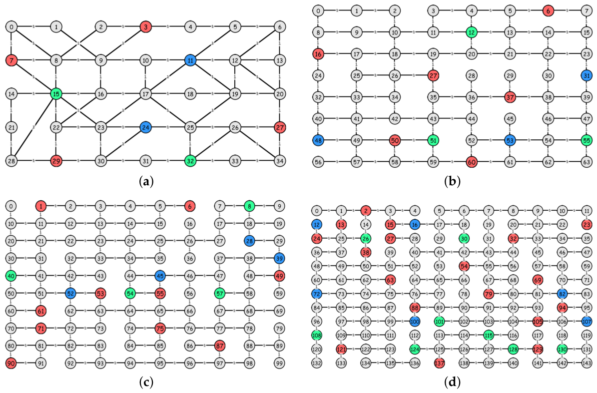
The four benchmark graphs are shown in Figure 2. Their grid layout is a pure choice of clarity, as it keeps the maps easy to visualize and the difficulty progression clear across G1-G4, with no loss of applicability to any other map. The proposed framework operates on an arbitrary connected weighted graph, since the DBT margin is computed by Dijkstra’s shortest-path distance over the edge weights W and the battery decay in (2) is proportional to those weights. The presence of obstacles is captured through graph connectivity, while factors such as physical distances or non-flat terrains (Figure 1) are captured through heterogeneous edge weights. The unit weights used in these four benchmarks are aimed at isolating the effect of graph connectivity and size on the recharging policy.
Across all benchmark graphs, the edge weights are assumed unitary and the battery decay dynamics are modeled according to the stochastic formulation (1). The nominal battery consumption is arbitrarily set to α = c 0 = 0.03 with stochastic perturbation σ = 0.005 and maximum decay Δ b max = 0.05 . Unless otherwise specified, the experimental section is based on the DBT reward function with safety designable parameters η = 1.5 and b o f f = 0 , fine-tuned to trade-off aggressiveness and conservativeness of the policy. After numerous trials, we found the sweet spot for η to be in the range 1.5 2.0 . A value of one degenerates in the nominal DBT, which does not sufficiently account for stochastic battery decay, while values greater than two tend to induce overly conservative policy behaviors.

4.2. Policies Implementation Details

The training algorithm was coded in PyTorch 2.3.1. The DDQN policy uses a Multi-Layer Perceptron (MLP) whose input and output dimensions match, respectively, the state- and action-space cardinality in (7) and (8). As the size of the environment increases, both the state and action spaces grow accordingly, leading to more complex state–action value approximations and longer training times. For this reason, different hidden-layer sizes are adopted for the MLP used in each benchmark graph, as summarized in Table 2. All neural networks use a LeakyReLU activation function with a negative slope of 0.1 . The reward parameters instantiate the magnitude ordering designed in (17) and are reported in Table 3. The learning hyperparameters, shared across all benchmark graphs, were instead obtained by fine-tuning and are listed in Table 4.

5. Numerical Results

5.1. Training and Monte Carlo Evaluation Across Graphs

We trained four DDQN policies with the DBT reward mechanism, one for each benchmark graph. To monitor training convergence, the networks were periodically evaluated on 30 random episodes, logging key performance metrics. In particular, we track the optimization objective—the maximization of the cumulative discounted reward (18)—and the episode success rate, which should converge to 100 % for a correct learning of the task. These quantities, together with the normalized episode length (scaled in [ 0 , K max ] with K max = 50 the unsuccessful truncation of the episode), are reported in Figure 3 for all benchmark graphs. All policies eventually reach a 100 % success rate, indicating that they learn to complete the site-servicing mission from any starting condition on the graph. As expected, training time increases with map complexity. The episodic reward follows a similar trend to the success rate, as the termination reward dominates the intermediate rewards. The normalized episode length also stabilizes as training progresses, with higher plateaus for more complex graphs due to longer trajectories. This analysis corroborates the convergence of the neural network training.
The training curves indicate a generally convergent learning process, but a more reliable assessment requires evaluation over a larger number of episodes and additional metrics. For this reason, each trained policy is tested on 10,000 Monte Carlo episodes, and the corresponding results are reported in Table 5. As expected, the episodic reward decreases with increasing graph complexity, mainly due to longer mission times and larger distances from charging stations. These factors raise the DBT (12), leading to more recharge stops, as reflected in the steadily increasing recharge rate from G1 to G4. The greater spatial complexity of the maps also results in a larger variance in episode length.
All policies achieve perfect mission Termination rate, meaning that the UAV always completes the site-servicing task with the correct tool. Most episodes also terminate with the positive reward (16), as indicated by the Positive Termination metric, which measures how often the final battery level remains above the DBT and is therefore sufficient to reach a charging station after having serviced the task. In a small fraction of episodes, the battery falls below the DBT due to stochastic fluctuations in the battery decay model. For these cases, we compute the safety margin as the difference between the actual battery level at termination and the nominal energy required to RTH, that is, the nominal DBT in (12). Across all benchmark maps, the safety margin remains strictly positive and sufficiently large, confirming that the gains and offset used in (12) to augment the nominal DBT provide an effective cushion against noise in the battery dynamics. Even when the battery terminates below the DBT, the UAV still retains enough nominal energy to reach a charging station, and the safety margin offers an additional buffer against stochastic variations during the RTH phase.
It is not meaningful in this evaluation setup to monitor whether the battery ever drops below zero during navigation: according to (5), the battery level can be artificially initialized near zero at the beginning of each episode, independently of the UAV’s proximity to charging nodes. Such events do not terminate the episode and therefore do not affect the validity of the reported metrics. Finally, all policies strictly respect the action feasibility constraints imposed by the environment, as no infeasible actions were observed throughout the entire Monte Carlo evaluation.

5.2. Sample DBT-DDQN Trajectories on Graphs

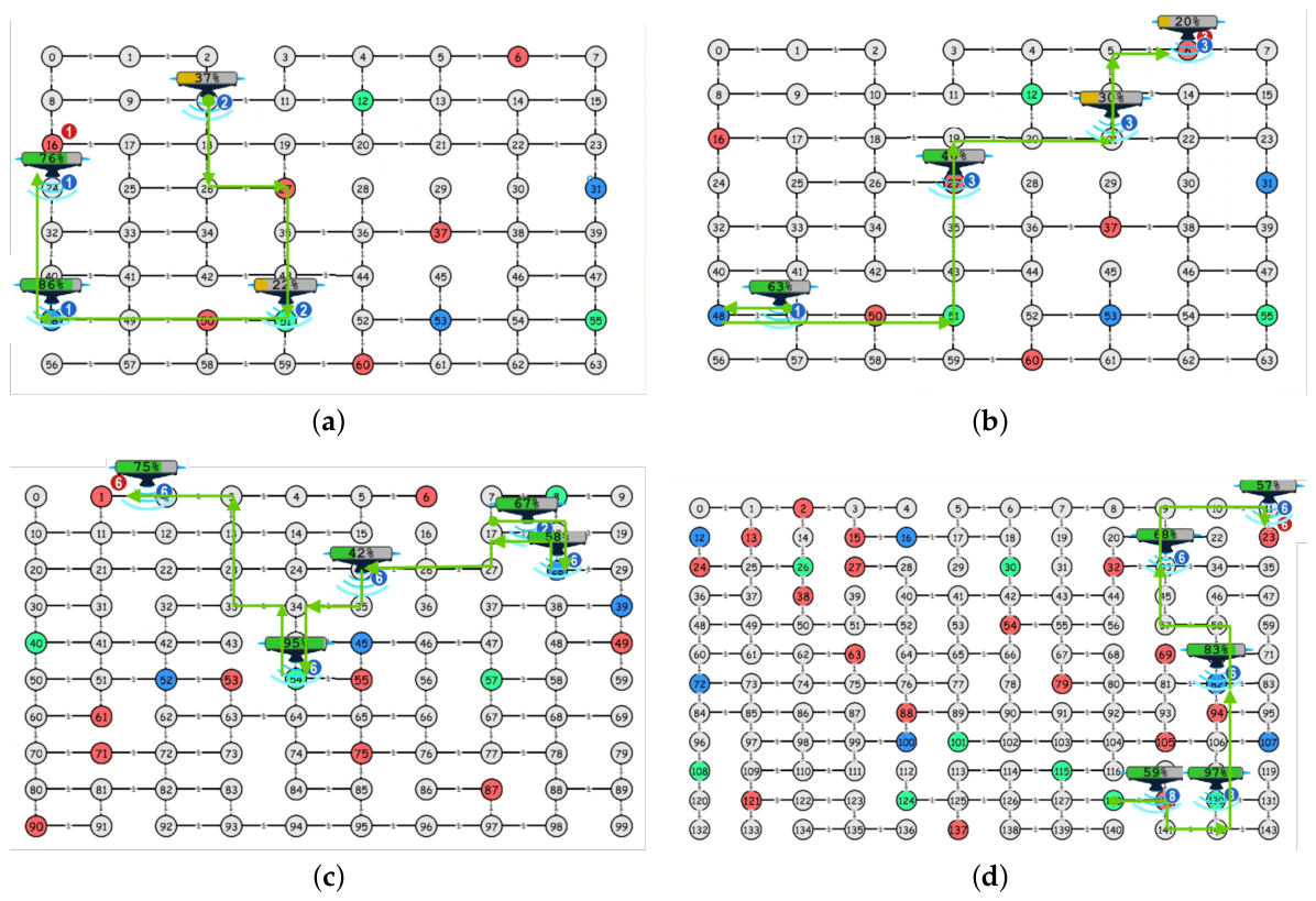
We present four emblematic and often occurring DBT-DDQN-controlled simulations on the more complex graphs G2, G3, G4. For a concise yet expressive depiction of the system’s evolution, we overlay the evolving MDP state onto the graph topology itself, yielding a compact visualization of the episode progression as in Figure 4. Here, a UAV is positioned on the graph with its battery and onboard tool depicted respectively with an overlying bar and a number aside, while the failure type is written next to the active target. As the state of the UAV is the only one varying during the episode, various frames of the UAV with its state are shown in different positions of the episodic trajectory, signaled with an oriented arrow moving along the graph’s edges.
In Figure 4a, the policy correctly identifies that changing the tool at depot node 48 and then heading directly to the failure location yields a very fast mission completion without risking discharge. However, the remaining battery after servicing would be insufficient to reach the closest charging station (node 51, seven steps away). Recharging immediately after the tool change would avoid this issue but would also increase the episode length (19 instead of 15 steps). The chosen trajectory is therefore optimal in expectation, according to (3), as it balances mission time and energy feasibility.
A similar averagely optimal behavior is displayed in Figure 4b, where the UAV starts close to depot node 48 and with enough battery, making the tool change the natural first action. The shortest path to the failure location crosses two charging stations, but the remaining battery after servicing the active task is still sufficient to reach station 12 under the adopted battery decay model. Recharging would only delay the mission. These two examples on graph G2 illustrate how the policy has learned when recharging is necessary and how to order recharge and tool-change operations depending on the map topology. Notably, in both cases, the UAV always follows the shortest paths between special nodes.
On the more complex graphs G3–G4, the DBT-DDQN policy continues to display desirable behaviors such as shortest-path navigation, sensible recharge decisions, and correct timing of tool changes, yet slight deviations from near-optimality occasionally emerge. In Figure 4c, the UAV correctly performs an early tool change and plans an intermediate recharge at node 54 before reaching the target, as the failure location is far from all charging stations. However, a faster solution would involve performing the tool change at node 45, which is very close to charging node 54, either before or after the recharge. This alternative would reduce the episode length from 21 to 19 steps. Such cases suggest a degree of myopic behavior: the network may struggle to distinguish small differences in long-term returns (the reward gap here is only six points), an aspect that warrants further investigation.
Finally, Figure 4d shows a simulation on G4, where the graph is less connected and special nodes are sparsely distributed, leaving large areas far from charging stations or depots. Despite this complexity, the policy adapts its conservative/aggressive balance to the map structure. Although the initial battery might seem sufficient to head directly to the failure location, node 23 is far from all charging stations, making the mission risky in terms of energy. The UAV would have enough battery to reach the target, but not to RTH afterwards. The policy foresees this and exploits the fact that the shortest path to the target passes by charging node 130, where it performs a recharge that avoids later detours and minimizes mission time. As also seen in Figure 4b, the policy does not adopt a simplistic “always recharge when passing by a station” strategy; instead, it effectively decides whether and when to recharge while pursuing the mission objective. This consistent behavior across scenarios indicates that DBT-DDQN achieves strong energy-awareness even on complex maps.

5.3. Ablation Study: Hidden MLP Size

One of the key design choices for achieving a competitive neural network policy lies in the size of the MLP. As the state and, especially, the action space expand with increasing environment complexity, it becomes progressively more challenging for the network to accurately approximate the quantity Q ( s , a ) . Adjusting the number of hidden neurons can therefore yield substantial improvements in mission-level performance, helping identify a suitable approximator for diverse graph environments.
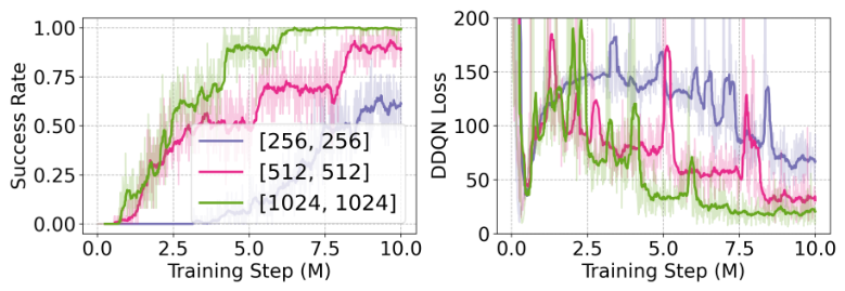
To validate this, we report training results for three different MLP hidden-layer sizes on the benchmark graph G3. The left-hand plot of Figure 5 shows that an inadequate choice of hidden dimensions leads to a severe drop in episode success rate, confirming that this parameter is critical and environment-dependent. For the graph considered, two hidden layers of 1024 neurons achieve a perfect success rate of 100 % , indicating that this configuration provides sufficient representational capacity. The right-hand plot illustrates the corresponding DDQN loss function (19), highlighting the superior approximation capability of the larger network, which yields the lowest loss and thus the most accurate representation of the state–action–reward space.
However, it remains unclear to what extent increasing the network size alone can influence the optimality properties of the learned policy. The comparison performed here is based exclusively on episode success rate, and therefore does not allow us to extrapolate conclusions on whether larger architectures systematically lead to higher returns beyond the observed improvements in task completion rate.

5.4. The Contribution of the DBT Reward

To isolate the contribution of the DBT reward term with respect to previously employed static thresholds [27], we compare the performance of DBT-DDQN with DDQN policies trained using fixed battery thresholds on the benchmark graphs. According to the notation in (15), this corresponds to setting b ̲ ( v k + 1 ) = b ̲ to a constant value. Our goal is to emulate a realistic continuous deployment scenario, in which the UAV is immediately given a new task after completing the previous one, navigating the graph to solve tasks sequentially while managing its battery across missions. This setup reflects practical operating conditions where the end state of one mission directly influences the next. To this end, we reset the full MDP state only for the first Monte Carlo test as in (5), while subsequent episodes start from the UAV state (battery, location, tool) reached at the end of the previous mission, resetting only the target node and failure type.
We trained DDQN networks with fixed thresholds b ̲ = { 0.15 , 0.20 , 0.25 , 0.30 } on graphs G2–G3, using the same training setup adopted for DBT-DDQN. These two maps were selected to limit training workload, and the threshold values were chosen based on the average distances from charging nodes in these environments. All fixed-threshold policies achieved 100 % success rate during training. We then evaluated them against DBT-DDQN in a Monte Carlo continuous deployment setting to assess whether DBT provides a notable advantage. Because each episode depends on the final state of the previous one, the stochastic seeds cannot be aligned across policies; therefore, we run 100 , 000 episodes to mitigate statistical variability.
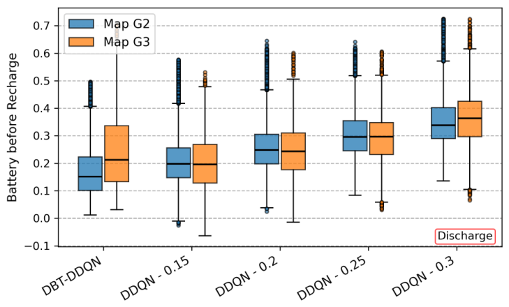
Figure 6 reports the distribution of battery levels before a recharge action for all policies on G2 and G3. As expected, the distributions shift upward as the static threshold increases. The lower quantiles and outliers are particularly informative: on G2, the DDQN-0.15 policy exhibits outliers below zero, meaning it would occasionally lead the UAV to discharge mid-mission and is therefore unsafe. Higher thresholds avoid negative outliers and provide increasing safety margins. DBT-DDQN never discharges during the entire continuous deployment experiment and achieves the lowest median battery-at-recharge, indicating that it learns to remain safe while avoiding excessive conservativeness.
This behavior appears consistently on both G2 and G3. Interestingly, for static-threshold policies, the median battery-at-recharge remains roughly constant across maps, showing that this naive approach is topology-unaware. However, their medians are significantly higher than that of DBT-DDQN, while their lower outliers approach or even fall below the zero-discharge boundary, suggesting that static thresholds fail to strike a balanced trade-off between conservativeness and aggressiveness. In contrast, DBT-DDQN adapts to the map structure and achieves a safer and more efficient recharge policy.
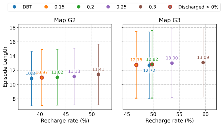
Figure 7 visualizes the Pareto-optimal trade-off between mission duration and recharge rate, i.e., the percentage of Monte Carlo runs in which the UAV first stops at a charging node. As above, results are reported under continuous deployment, where each episode starts from the final state of the previous one. On G2, DBT-DDQN is Pareto-optimal with respect to the fixed-threshold policies: it learns to recharge only when necessary and achieves the lowest average episode length, with a variability comparable across all methods. As the static threshold increases, the average episode length also increases, indicating a progressively more conservative behavior. On G3, DBT is Pareto-optimal among the policies that never discharge during continuous deployment. In this map, the lower thresholds 0.15 and 0.20 are too aggressive to cope with the larger distances from the more sparse charging stations, and they occasionally lead to battery depletion.

5.5. Pseudo-Optimality Analysis

Assessing the optimality of the proposed DBT-DDQN across different maps is computationally intractable, as the cost of an exhaustive search grows combinatorially. A meaningful and computationally feasible baseline for comparison is instead provided by a look-ahead planner based on Monte Carlo Tree Search (MCTS). The MCTS method approximates the optimal solution by deterministically exploring the decision tree and evaluating future action sequences through rollout simulations. For fairness, the planner maximizes the cumulative reward over a finite horizon, which, when chosen sufficiently large, covers the entire mission duration for all benchmark maps. Although MCTS generally offers strong planning performance, its computational complexity increases rapidly with both the branching factor and the planning horizon. To mitigate this effect, especially in larger graphs, the expansion policy evaluates rollouts only over the feasible action subset (9), significantly reducing the branching factor while preserving meaningful planning trajectories. In all experiments, the pruning parameter and the planning horizon were set to 150 and 20, respectively, representing a compromise between solution quality and tractability. Larger parameters in this regard would push MCTS closer to the true optimum, but at a cost that grows rapidly and that, beyond the practical infeasibility of running online, would make the Monte Carlo campaign itself prohibitive. The chosen setting already places MCTS in the near-optimal regime, as confirmed by the following experiments, so a larger budget would trade large runtime increases for marginal gains without altering the conclusions.
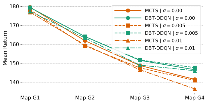
The comparison between DBT-DDQN and MCTS is conducted over 1000 independent tests, resetting the full environment state between episodes to ensure identical scenarios for both methods. Since MCTS is deterministic while the environment is stochastic, its planning is expected to be more exposed to model inaccuracy; in the following, we retain the deterministic MCTS formulation, as averaging multiple rollouts per action would further increase its already important computational cost. The evaluation spans all benchmark maps and three levels of stochastic battery decay, σ = { 0.00 , 0.005 , 0.01 } , to assess both optimality and robustness. The mean return over the 10 , 000 episodes is shown in Figure 8. The two methods perform similarly on the simplest map G1, suggesting that this value may be close to the theoretical optimum. As map complexity increases, the performance gap widens. One interpretation is that this gap reflects the distance between the pseudo-optimal MCTS and the true optimum, with the planner degrading as complexity rises. However, this contrasts with earlier observations indicating that DBT-DDQN also exhibits non-optimal behaviors (e.g., the trajectory in Figure 4c). Although DBT-DDQN may not be fully optimal on complex maps, its performance degrades less than that of MCTS, whose pseudo-optimality is given by pruning and the finite planning horizon. In this sense, the DBT-DDQN policy can be considered, on average, closer to the theoretical optimum than the look-ahead planner.
Figure 8 also serves as a robustness check against inaccuracy in the energy model (1). At every map, the DBT-DDQN return stays tightly clustered for the deterministic and low-noise cases, and it crucially holds at σ = 0.01 , above the noise value used in training, indicating that the policy tolerates energy dynamics it did not encounter during learning. The pseudo-optimal MCTS planner, by contrast, is expectedly more exposed to σ : its gap from the deterministic model widens across noise levels and map complexity. Moreover, MCTS is matched or outperformed by DBT-DDQN in every stochastic regime on every map, suggesting greater robustness to model uncertainties.
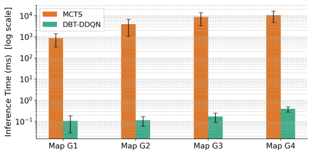
To further promote the practical relevance of DBT-DDQN, we report the inference time measured during the Monte Carlo evaluation. One of the main advantages of RL-based controllers over optimization-based planners is their substantially lower computational burden. The inference time is computed using Python’s time.perf_counter and refers to the same hardware used for training: an Ubuntu server equipped with an AMD EPYC 7413 24-Core CPU and 1 TB RAM, which enabled fast training and evaluation. The mean and standard deviation of the inference time are shown in Figure 9. The two methods differ by four orders of magnitude: even with the largest network (G4), DBT-DDQN produces an action in less than one millisecond on this high-performance machine, and likely within a few tens of milliseconds on a low-cost onboard processor, making it suitable for real-time deployment even in complex environments. In contrast, the inference time of MCTS quickly grows to several seconds, which severely limits its feasibility in real-world scenarios. Considering the reduced computational load, the near-optimality observed with respect to the look-ahead planner, and the superior robustness to environmental stochasticity, these factors collectively support the use of DBT-DDQN as an efficient decision-maker on graphs, capable of balancing mission performance and energy-awareness.

6. Discussions and Conclusions

This paper addressed the problem of energy-aware site-servicing for a UAV navigating on a graph map, where the agent must collect the appropriate tool, deliver it to an active failure node, and autonomously manage recharge stops so as to minimize mission duration while avoiding battery depletion. The problem was formulated as an MDP and solved via the DDQN algorithm, whose central contribution is a Dynamic Battery-Threshold (DBT-DDQN) reward mechanism derived from the shortest-path distance to the nearest recharge station. Extensive Monte Carlo simulations show that, unlike fixed-threshold approaches, the DBT reward adapts to the map topology at each decision step, enabling the agent to strike a better balance between episode duration and battery safety across graphs of increasing complexity. For multi-objective UAV routing problems on graph maps, DDQN proves highly effective: the learned policy achieves 100 % success rates on all benchmark maps, scales gracefully with state and action space size, and is more robust to stochastic model parameters (for the energy consumption) than an MCTS planner, whose performance degrades more rapidly with map size.
Despite these results, two limitations deserve acknowledgment. The position of DBT-DDQN relative to the theoretical optimum remains uncertain on larger graphs: comparisons with MCTS suggest near-optimality, but cannot guarantee proximity to the true optimum. Moreover, when far from the target, the agent occasionally exhibits suboptimal behaviors, such as unnecessary detours for recharging or non-ideal choices of nodes for tool changes (Figure 4c), indicating that the current feedforward architecture may be inherently myopic for high-dimensional, long-horizon instances.
Nonetheless, the proposed method demonstrates strong and consistent capabilities. DBT-DDQN reliably identifies whether and when to recharge along the path to the target (Figure 4b,d), always navigates through shortest paths between nodes, and achieves perfect mission success even on the largest benchmark maps. This, together with its robustness to model inaccuracy (Figure 8) and its far lower inference cost (Figure 9) compared to the look-ahead planner, confirms that the learned policy is a strong and practical solution for balancing mission performance and energy-awareness in UAV graph routing.
Building on these findings, several directions emerge for future research. From an algorithmic standpoint, the approximation capacity of the policy could be enhanced through larger, recurrent, or attention-based architectures better suited to long-horizon planning. On the mission side, the framework could be extended to richer objective structures and, ultimately, to the multi-agent setting, where multiple UAVs coordinate through a two-level architecture combining an external task-assignment loop with a DBT-DDQN-like execution policy. On the evaluation side, the method should be tested on graphs with heterogeneous edge weights and with higher-fidelity energy consumption and non-instantaneous recharge models, all already supported by the construction of the method.

Author Contributions

Conceptualization, G.G. and L.P.; methodology, G.G.; software, G.G.; validation, G.G.; formal analysis, G.G.; investigation, G.G.; resources, G.G.; data curation, G.G.; writing—original draft preparation, G.G.; writing—review and editing, G.G. and L.P.; visualization, G.G. and L.P.; supervision, G.G. and L.P.; project administration, L.P.; funding acquisition, L.P. All authors have read and agreed to the published version of the manuscript.

Funding

Project co-funded by the European Union—Next Generation EU—under the National Recovery and Resilience Plan (NRRP), Mission 4 Component 1 Investment 4.1—Decree No. 118 (2nd March 2023) of the Italian Ministry of University and Research—Concession Decree No. 2333 (22nd December 2023), Project code D93C23000450005, within the Italian National Program PhD Programme in Autonomous Systems (DAuSy).

Institutional Review Board Statement

Not applicable.

Informed Consent Statement

Not applicable.

Data Availability Statement

The raw data and software supporting the conclusions of this article will be made available by the authors on request.

Acknowledgments

During the preparation of this manuscript, the authors used ChatGPT-4o to generate the background landscape in Figure 1. The authors have reviewed and edited the output and take full responsibility for the content of this publication.

Conflicts of Interest

The authors declare no conflicts of interest.

Abbreviations

The following abbreviations are used in this manuscript:
UAVUnmanned Aerial Vehicle
DDQNDouble Deep Q-Network
DBTDynamic Battery Threshold
RLReinforcement Learning
MDPMarkov Decision Process
MLPMulti-Layer Perceptron
MCTSMonte Carlo Tree Search
PERPrioritized Experience Replay
MILPMixed-Integer Linear Programming
UGVUnmanned Ground Vehicle
RTHReturn To Home
PPOProximal Policy Optimization
IDDQNImproved Double Deep Q-network

References

  1. Mohsan, S.A.H.; Othman, N.Q.H.; Li, Y.; Alsharif, M.H.; Khan, M.A. Unmanned aerial vehicles (UAVs): Practical aspects, applications, open challenges, security issues, and future trends. Intell. Serv. Robot. 2023, 16, 109–137. [Google Scholar] [CrossRef] [PubMed]
  2. Bouček, Z.; Flídr, M. Mission Planner for UAV Battery Replacement. In Proceedings of the 2024 IEEE International Conference on Multisensor Fusion and Integration for Intelligent Systems (MFI), Pilsen, Czech Republic, 4–6 September 2024; pp. 1–6. [Google Scholar] [CrossRef]
  3. Zeng, Y.; Zhang, R. Energy-efficient UAV communication with trajectory optimization. IEEE Trans. Wirel. Commun. 2017, 16, 3747–3760. [Google Scholar] [CrossRef]
  4. Theile, M.; Bayerlein, H.; Nai, R.; Gesbert, D.; Caccamo, M. UAV Coverage Path Planning under Varying Power Constraints using Deep Reinforcement Learning. In Proceedings of the 2020 IEEE/RSJ International Conference on Intelligent Robots and Systems (IROS), Las Vegas, NV, USA, 25–29 October 2020; pp. 1444–1449. [Google Scholar] [CrossRef]
  5. Theile, M.; Bayerlein, H.; Caccamo, M.; Sangiovanni-Vincentelli, A.L. Learning to recharge: UAV coverage path planning through deep reinforcement learning. arXiv 2023, arXiv:2309.03157. [Google Scholar]
  6. Zhang, Y.; Zheng, H.; Zhai, X. Deep Reinforcement Learning Based UAV Mission Planning with Charging Module. In Proceedings of the 2023 4th International Conference on Computing, Networks and Internet of Things, Xiamen, China, 26–28 May 2023; pp. 658–662. [Google Scholar]
  7. Grando, L.; Jaramillo, J.F.G.; Leite, J.R.E.; Ursini, E.L. Modeling and Simulation of Battery Recharging for UAVs Applications: Smart Farming, Disaster Recovery, and Dengue Focus Detections. In Proceedings of the 2024 Winter Simulation Conference (WSC); IEEE: Piscataway, NJ, USA, 2024; pp. 2832–2843. [Google Scholar]
  8. Garey, M.R.; Johnson, D.S. A Guide to the Theory of NP-Completeness. In Computers and Intractability; W.H. Freeman and Company: New York, NY, USA, 1990; pp. 37–79. [Google Scholar]
  9. Sundar, K.; Rathinam, S. Algorithms for routing an unmanned aerial vehicle in the presence of refueling depots. IEEE Trans. Autom. Sci. Eng. 2013, 11, 287–294. [Google Scholar] [CrossRef]
  10. Ribeiro, R.G.; Cota, L.P.; Euzébio, T.A.M.; Ramírez, J.A.; Guimarães, F.G. Unmanned-Aerial-Vehicle Routing Problem With Mobile Charging Stations for Assisting Search and Rescue Missions in Postdisaster Scenarios. IEEE Trans. Syst. Man Cybern. Syst. 2022, 52, 6682–6696. [Google Scholar] [CrossRef]
  11. Yu, K.; Budhiraja, A.K.; Tokekar, P. Algorithms for Routing of Unmanned Aerial Vehicles with Mobile Recharging Stations. In Proceedings of the 2018 IEEE International Conference on Robotics and Automation (ICRA), Brisbane, Australia, 21–25 May 2018; pp. 5720–5725. [Google Scholar] [CrossRef]
  12. Alyassi, R.; Khonji, M.; Karapetyan, A.; Chau, S.C.K.; Elbassioni, K.; Tseng, C.M. Autonomous Recharging and Flight Mission Planning for Battery-Operated Autonomous Drones. IEEE Trans. Autom. Sci. Eng. 2023, 20, 1034–1046. [Google Scholar] [CrossRef]
  13. Mohabbati-Kalejahi, N.; Alavi, S.; Toragay, O. A mixed-integer programming framework for drone routing and scheduling with flexible multiple visits in highway traffic monitoring. Mathematics 2025, 13, 2427. [Google Scholar] [CrossRef]
  14. Ramasamy, S.; Reddinger, J.P.F.; Dotterweich, J.M.; Childers, M.A.; Bhounsule, P.A. Cooperative route planning of multiple fuel-constrained unmanned aerial vehicles with recharging on an unmanned ground vehicle. In Proceedings of the 2021 International Conference on Unmanned Aircraft Systems (ICUAS); IEEE: Piscataway, NJ, USA, 2021; pp. 155–164. [Google Scholar]
  15. Maini, P.; Sundar, K.; Singh, M.; Rathinam, S.; Sujit, P.B. Cooperative Aerial–Ground Vehicle Route Planning With Fuel Constraints for Coverage Applications. IEEE Trans. Aerosp. Electron. Syst. 2019, 55, 3016–3028. [Google Scholar] [CrossRef]
  16. Chen, Z.; Hu, Z.; Bao, Z.; Xu, W. UAV Charging Station Planning and Route Optimization Considering Stochastic Delivery Demand. IEEE Trans. Transp. Electrif. 2024, 10, 9328–9341. [Google Scholar] [CrossRef]
  17. Fagundes-Junior, L.A.; de Carvalho, K.B.; Ferreira, R.S.; Brandão, A.S. Machine learning for unmanned aerial vehicles navigation: An overview. SN Comput. Sci. 2024, 5, 256. [Google Scholar] [CrossRef]
  18. Zhao, C.; Liu, J.; Yoon, S.U.; Li, X.; Li, H.; Zhang, Z. Energy constrained multi-agent reinforcement learning for coverage path planning. In Proceedings of the 2023 IEEE/RSJ International Conference on Intelligent Robots and Systems (IROS); IEEE: Piscataway, NJ, USA, 2023; pp. 5590–5597. [Google Scholar]
  19. Fu, H.; Li, Z.; Zhang, W.; Feng, Y.; Zhu, L.; Long, Y.; Li, J. Path Planning for Agricultural UAVs Based on Deep Reinforcement Learning and Energy Consumption Constraints. Agriculture 2025, 15, 943. [Google Scholar] [CrossRef]
  20. Fan, M.; Wu, Y.; Liao, T.; Cao, Z.; Guo, H.; Sartoretti, G.; Wu, G. Deep Reinforcement Learning for UAV Routing in the Presence of Multiple Charging Stations. IEEE Trans. Veh. Technol. 2023, 72, 5732–5746. [Google Scholar] [CrossRef]
  21. Ni, J.; Gu, Y.; Gu, Y.; Zhao, Y.; Shi, P. UAV coverage path planning with limited battery energy based on improved deep double Q-network. Int. J. Control Autom. Syst. 2024, 22, 2591–2601. [Google Scholar] [CrossRef]
  22. Chu, N.H.; Hoang, D.T.; Nguyen, D.N.; Van Huynh, N.; Dutkiewicz, E. Joint Speed Control and Energy Replenishment Optimization for UAV-Assisted IoT Data Collection with Deep Reinforcement Transfer Learning. IEEE Internet Things J. 2023, 10, 5778–5793. [Google Scholar] [CrossRef]
  23. Li, X.; Yao, L.; Li, M.; Zhang, B. Reinforcement Learning Based Collaborative Path Planning Research for UAVs and Unmanned Vehicles. In Proceedings of the International Conference on Machine Learning and Intelligent Computing; PMLR: Cambridge, MA, USA, 2025; pp. 595–603. [Google Scholar]
  24. Mondal, M.S.; Ramasamy, S.; Bhounsule, P. OptiRoute: A Heuristic-assisted Deep Reinforcement Learning Framework for UAV-UGV Collaborative Route Planning. arXiv 2023, arXiv:2309.09942. [Google Scholar]
  25. Mondal, M.S.; Ramasamy, S.; Humann, J.D.; Dotterweich, J.M.; Reddinger, J.P.F.; Childers, M.A.; Bhounsule, P. An attention-aware deep reinforcement learning framework for uav-ugv collaborative route planning. In Proceedings of the 2024 IEEE/RSJ International Conference on Intelligent Robots and Systems (IROS); IEEE: Piscataway, NJ, USA, 2024; pp. 13687–13694. [Google Scholar]
  26. Mondal, M.S.; Ramasamy, S.; Rownak, R.; Russo, L.; Humann, J.D.; Dotterweich, J.M.; Bhounsule, P. Risk-Aware Energy-Constrained UAV-UGV Cooperative Routing Using Attention-Guided Reinforcement Learning. In Proceedings of the 2025 IEEE International Conference on Robotics and Automation (ICRA); IEEE: Piscataway, NJ, USA, 2025; pp. 13000–13006. [Google Scholar]
  27. Gemignani, G.; Bongiorni, M.; Pollini, L. An Energy-aware Decision-making scheme for Mobile Robots on a Graph map based on Deep Reinforcement Learning. In Proceedings of the 2024 18th International Conference on Control, Automation, Robotics and Vision (ICARCV); IEEE: Piscataway, NJ, USA, 2024; pp. 460–466. [Google Scholar]
  28. Van Hasselt, H.; Guez, A.; Silver, D. Deep reinforcement learning with double q-learning. In Proceedings of the AAAI Conference on Artificial Intelligence, Phoenix, AZ, USA, 12–17 February 2016; Volume 30. [Google Scholar]
  29. Meng, W.; Zhang, X.; Zhou, L.; Guo, H.; Hu, X. Advances in UAV path planning: A comprehensive review of methods, challenges, and future directions. Drones 2025, 9, 376. [Google Scholar] [CrossRef]
  30. Dai, W.; Rai, U.; Chiun, J.; Cao, Y.; Sartoretti, G. Heterogeneous multi-robot task allocation and scheduling via reinforcement learning. IEEE Robot. Autom. Lett. 2025, 10, 2654–2661. [Google Scholar] [CrossRef]
  31. Gemignani, G.; Casini, S.; Rosellini, V.; Bucchioni, G.; Pollini, L. Preliminary Design of Human-like Decentralised Task Assignment for Heterogeneous Unmanned Vehicles using Reinforcement Learning. In Proceedings of the AIAA SCITECH 2026 Forum, Orlando, FL, USA, 12–16 January 2026; p. 0326. [Google Scholar]
  32. Mnih, V.; Kavukcuoglu, K.; Silver, D.; Rusu, A.A.; Veness, J.; Bellemare, M.G.; Graves, A.; Riedmiller, M.; Fidjeland, A.K.; Ostrovski, G.; et al. Human-level control through deep reinforcement learning. Nature 2015, 518, 529–533. [Google Scholar] [CrossRef] [PubMed]
  33. Dijkstra, E.W. A note on two problems in connexion with graphs. In Edsger Wybe Dijkstra: His Life, Work, and Legacy; Association for Computing Machinery (ACM): New York, NY, USA; Morgan & Claypool: New York, NY, USA, 2022; pp. 287–290. [Google Scholar]
  34. Schaul, T.; Quan, J.; Antonoglou, I.; Silver, D. Prioritized experience replay. arXiv 2015, arXiv:1511.05952. [Google Scholar]
  35. Towers, M.; Kwiatkowski, A.; Balis, J.; De Cola, G.; Deleu, T.; Goulão, M.; Andreas, K.; Krimmel, M.; Kg, A.; Perez-Vicente, R.; et al. Gymnasium: A standard interface for reinforcement learning environments. Adv. Neural Inf. Process. Syst. 2026, 38. [Google Scholar] [CrossRef]
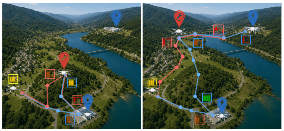
Figure 1. (The background of this image was AI-generated) Illustration of the trade-off between mission efficiency and battery safety in UAV task-servicing over the same environment, under two different task configurations (left and right panels). In each panel, two policies are depicted: an aggressive policy (red trajectory) and a conservative one (blue trajectory), visiting waypoints (circles of the same color as the trajectory). Both UAVs must visit task sites (red pins) and recharge stations (blue pins), starting from the same position with the same initial battery level (yellow border). Colored squares alongside the paths denote the observed battery level at each visited node, with border color matching the corresponding trajectory. In one configuration (left), the aggressive policy completes the mission faster, while in the other (right) it risks battery depletion before reaching the nearest recharge station. The desired policy should find the optimal compromise between these two behaviors depending on the environment topology and the current agent-task state.
Electronics 15 02984 g001
Figure 2. Benchmark graphs used in simulations. Nodes are numbered in a grid layout. Special nodes are red (targets), blue (depots), and green (charging stations). Edge weights are unitary and indicated over the edges. (a) G1. (b) G2. (c) G3. (d) G4.
Electronics 15 02984 g002
Figure 3. Training curves for the four benchmark maps (from left to right: G1–G4). The 10-point moving average is shown as a solid line, while raw data appear as a shaded trace. For a uniform y-axis scale, the episodic reward is clipped to [ 200 , 200 ] (the scale of the termination rewards (16)) and then normalized to [ 0 , 1 ] . The normalized episode length (scaled in [ 0 , 50 ] ) is also displayed.
Electronics 15 02984 g003
Figure 4. DBT-DDQN policy simulation on G2 (a,b), G3 (c) and G4 (d). Nodes are numbered in a grid layout. Special nodes are red (targets), blue (depots), and green (charging stations). Edge weights are unitary and indicated over the edges. The active target is indicated with a red circle next to the node reporting the failure number, and the same mechanism is adopted for the tool carried by the UAV, but with a blue circle. The UAV is depicted at different times during the trajectory, the latter visualized with the oriented green arrow. Over the UAV, a battery bar indicates the % level of remaining charge.
Electronics 15 02984 g004
Figure 5. Training curves for different hidden MLP sizes on benchmark graph G3.
Electronics 15 02984 g005
Figure 6. Battery level before recharge actions: distribution across dynamic (DBT) and static threshold policies, experiments on maps G2–G3. Data is gathered on 100 , 000 tests carried out in continuous deployment conditions.
Electronics 15 02984 g006
Figure 7. Mission duration mean and std vs. recharge rate (% of episodes) scatter across dynamic (DBT) and static threshold policies; experiments on maps G2–G3. Data is gathered on 100,000 tests carried out in continuous deployment conditions.
Electronics 15 02984 g007
Figure 8. Mean return over 10,000 independent episodes for DBT-DDQN and MCTS policies across various benchmark maps and battery decay standard deviation.
Electronics 15 02984 g008
Figure 9. Mean and std of decision-making inference time over 10,000 independent episodes for DBT-DDQN and MCTS policies across various benchmark maps.
Electronics 15 02984 g009
Table 1. Graph parameters used in the simulation campaign.
GraphN | V t | | V d | | V c | M p conn
G1354223/
G26463350.80
G3100104460.75
G4144186880.70
/ denotes a hand-tailored configuration.
Table 2. State-space, action-space, and MLP hidden-layer dimensions for each graph.
GraphState Dim.Action Dim.MLP
G11340 [ 256 , 256 ]
G21671 [ 512 , 512 ]
G318108 [ 1024 , 1024 ]
G421154 [ 2048 , 2048 ]
Table 3. Reward parameters, instantiating the ordering of (17).
Parameter R term c inf c DBT c rech c move
Value2005025103
Table 4. DDQN training hyperparameters.
HyperparameterValueHyperparameterValue
Learning rate 5 × 10 4 Batch size128
Exploration factor ε 0.3 Buffer size 1 × 10 6
Target network sync rate 1 × 10 3 Discount factor 0.99
Environment transitions per step10PER priority exponent [34] 0.65
PER importance sampling [34] 0.80 Backpropagation optimizerAdamW
Table 5. Monte Carlo Evaluation for DBT-DDQN policies on benchmark environments G1–G4.
MetricG1G2G3G4
Episodic reward (mean ± std)178.15 ± 20.85162.82 ± 29.32152.18 ± 41.59140.75 ± 51.24
Episode length (mean ± std)7.26 ± 2.1911.21 ± 3.8112.92 ± 4.2915.84 ± 5.74
Termination rate (%)100.00100.00100.00100.00
Infeasible actions rate (%)0.000.000.000.00
Recharges rate (%)26.5542.1553.1855.96
Positive termination rate (16) (%)99.97100.0099.9999.88
Safety battery margin range *[0.029, 0.041]/[0.051, 0.051][0.011, 0.119]
* Computed when episode terminates with battery lower than the DBT (12).
Disclaimer/Publisher’s Note: The statements, opinions and data contained in all publications are solely those of the individual author(s) and contributor(s) and not of MDPI and/or the editor(s). MDPI and/or the editor(s) disclaim responsibility for any injury to people or property resulting from any ideas, methods, instructions or products referred to in the content.