CSA-PTR: Context-Aware Feature Splitting and Polarized Topology Refinement for Reliable Selective Propagation in Graph Neural Networks

Abstract

Graph Neural Networks (GNNs) have achieved strong performance on graph-structured data via neighborhood message passing. Recent studies on GNNs suggest that not all feature dimensions benefit equally from message passing, motivating preference-guided feature splitting rather than uniform aggregation. Empirically, the splitting criterion is affected by class-boundary nodes with label-inconsistent neighborhoods, which confound the estimation of which dimensions should be propagated. Moreover, conducting propagation on the original topology may amplify feature–topology mismatch, causing messages to be passed along incompatible edges. To address these issues, we propose a plug-and-play architecture called Core–Shell Adaptive augmentation with dual-branch Polarized Topology Refinement (CSA-PTR), through simultaneous consideration of clearer feature splitting and a more ideal topology for GNNs to better satisfy the selective propagation criterion. Specifically, CSA-PTR consists of three modules. Core–shell adaptive augmentation stabilizes node representations by a purity-aware clustering algorithm, which reduces the ambiguity in feature-preference estimation. Then, graph feature splitting allocates feature dimensions into a propagation branch and a feature-only branch based on learned preferences. Finally, Dual-branch Polarized Topology Refinement exploits these branches as complementary views to learn polarized weights, yielding a more desirable topology and improving information flow. Extensive experiments on diverse benchmarks show that CSA-PTR achieves competitive performance across the evaluated settings, while consistently improving several representative GNN backbones.

1. Introduction

Graph Neural Networks (GNNs) have emerged as a prominent paradigm for representation learning on graph-structured data [1], demonstrating strong effectiveness in modeling complex relationships in domains, such as recommendation systems [2,3], molecular graphs [4,5], and traffic forecasting [6,7,8]. In general, GNNs learn node representations through iterative neighborhood message passing [9], which enables them to incorporate structural information into node embeddings.

Despite their success, message passing is not universally beneficial [10]. When information is propagated indiscriminately, GNNs may over-smooth discriminative signals or aggregate messages along task-irrelevant edges, especially when the graph topology is not well aligned with feature semantics [11]. These limitations have motivated increasing interest in selective propagation, which applies graph convolution only when it is truly beneficial.

Recent studies have progressively refined the criteria for selective propagation. Early works revisited the conditions under which graph-aware models improve node classification and proposed more informative measures for assessing the benefits of graph convolution [12,13]. Subsequent studies further showed that these benefits are shaped by the interaction between graph topology and node features [14]. Building on this view, more recent feature-splitting frameworks have pushed the analysis to the feature-dimension level. One representative framework introduces Topological Feature Informativeness (TFI) to distinguish GNN-favored and GNN-disfavored dimensions, enabling split processing with graph-based and graph-agnostic models [15].

However, existing selective propagation frameworks still exhibit a gap between their underlying principles and their behavior on realistic graphs. In particular, although feature splitting is intended to identify dimensions that are more suitable for graph convolution, its estimation process can be unreliable in structurally complicated regions, and directly reusing the original topology after splitting may still introduce incompatible propagation paths. These issues call for a closer empirical examination before further architectural design.

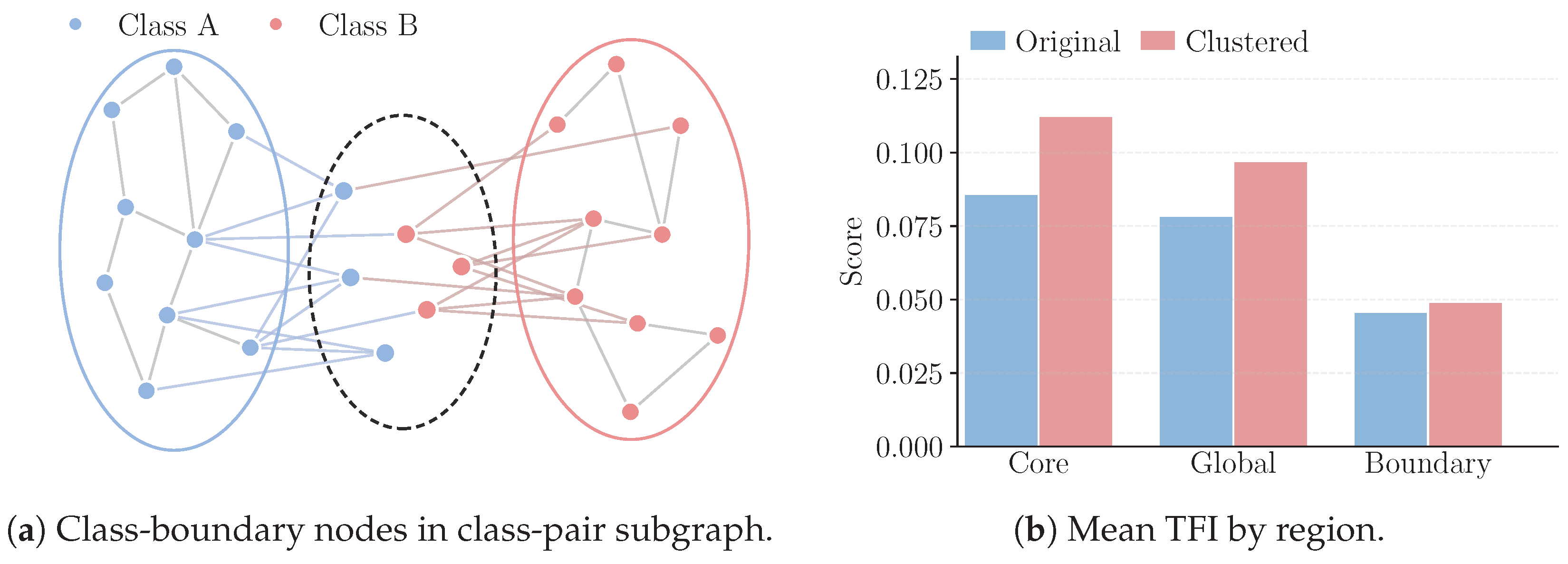
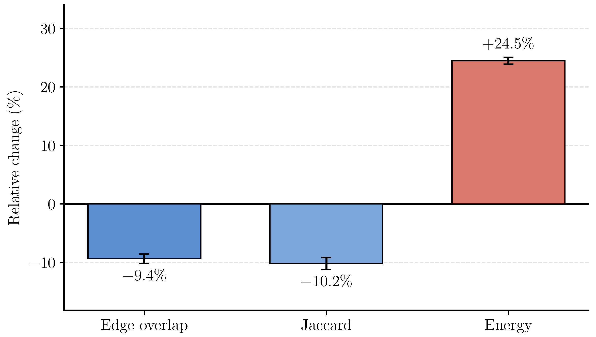
To clarify this gap, we conduct two preliminary experiments. First, as shown in Figure 1, nodes near class boundaries, which often exhibit label-inconsistent neighborhoods, consistently show lower TFI-related informativeness than other regions. This suggests that directly mixing untreated boundary nodes into the overall estimation may dilute the estimated informativeness of candidate propagation dimensions and thus bias the split criterion. Second, as shown in Figure 2, we assess feature–topology compatibility by comparing the original graph with the feature-induced kNN graph through Edge Overlap [16] and Jaccard similarity [17], and by further measuring feature smoothness with Dirichlet energy [18]. The results indicate that feature splitting weakens the alignment between the split features and the original topology, revealing a clear feature–topology mismatch. Such a mismatch may hinder effective message passing in GNNs when propagation is still performed on the unchanged graph structure.

Taken together, these observations suggest that improving feature-splitting GNNs requires intervention at two stages. The first is the estimation stage, where propagation-favored dimensions are identified and can be biased by locally mixed neighborhoods. The second is the propagation stage, where the selected graph-favored features interact with the graph structure and may suffer from topology mismatch if the original graph is directly reused.

To address these challenges, we develop a plug-and-play architecture called CoreShell Adaptive augmentation with dual-branch Polarized Topology Refinement (CSA-PTR), which enhances a feature-splitting pipeline from both the estimation and propagation perspectives. Specifically, the core–shell adaptive augmentation module uses purity-aware clustering to reduce the ambiguity introduced by class-boundary nodes, leading to more stable feature-preference estimation. Based on these refined preferences, the feature-splitting process divides feature dimensions into a propagation branch and a feature-only branch, so that message passing is reserved for dimensions that are more likely to benefit from graph convolution. To further alleviate feature–topology mismatch, the Dual-branch Polarized Topology Refinement module treats these two branches as complementary views and learns polarized edge weights, yielding a more desirable topology for information flow. Through this coordinated design, CSA-PTR improves both the reliability of feature-preference estimation and the suitability of propagation paths, making selective propagation more effective on realistic graphs. Our main contributions are summarized as follows:

(1)

We identify two coupled issues of feature-splitting GNNs on realistic graphs: biased estimation of propagation-favored dimensions in locally mixed boundary regions, and feature–topology mismatch caused by directly reusing the original graph after feature splitting.

(2)

We propose a coordinated framework, CSA-PTR, for feature-splitting GNNs on realistic graphs. Rather than modifying the original splitting criterion itself, CSA improves the contextual basis on which feature-wise propagation preference is estimated, while DPTR refines the propagation topology used by the split graph-favored branch through polarized relation modeling and dual-branch coordination.

(3)

We provide extensive empirical evaluation on multiple benchmark datasets, including low-label settings, an ablation study, statistical comparison, and a framework study, showing that CSA-PTR achieves competitive and generally superior performance across the evaluated settings.

The rest of this paper is organized as follows. In Section 2, we review related work on graph convolution, selective propagation, and polarization in GNNs. In Section 3, we introduce the proposed CSA-PTR framework in detail, and in Section 4, we report the experimental results and further analysis. Finally, Section 5 presents the conclusion and outlines future work.

2. Related Work

2.1. Graph Convolution and Selective Propagation

GNNs have been predominantly developed under the message-passing paradigm, where node representations are learned by aggregating information from neighboring nodes over the graph structure. Early representative models, such as GCN [19] and GAT [20], established the basic framework of neighborhood aggregation and demonstrated the effectiveness of graph convolution for node representation learning. Building on this foundation, a large body of work has focused on improving how information is propagated, for example through subgraph sampling in GraphSAINT [21] and high-order propagation in MixHop [22].

Despite these successes, most conventional GNNs still implicitly assume that neighborhood propagation is broadly beneficial to representation learning. However, this assumption does not always hold in realistic graphs. When graph topology is weakly aligned with feature semantics, indiscriminate message passing may over-smooth discriminative signals, thereby degrading downstream performance. To address these limitations, recent studies have moved beyond improving propagation strength alone and begun to investigate selective propagation.

Earlier method-oriented studies mainly focused on adapting propagation to local graph contexts, rather than enforcing a single propagation rule for all nodes. For instance, Ada-GNN learns subgroup-specific personalized models to better capture local patterns, while node-wise architecture methods further assign different propagation depths, aggregators, and resolutions to different nodes according to their local structures [23,24]. More recently, representative feature-splitting frameworks introduce Topological Feature Informativeness (TFI) to identify which dimensions are more suitable for graph convolution and which are better preserved without propagation, thereby enabling more fine-grained selective processing [15]. However, existing feature-splitting methods mainly focus on determining which feature dimensions should be propagated, while paying less attention to whether this preference can be estimated reliably in locally mixed regions and whether the original topology remains suitable after splitting. In contrast, our work focuses on two practical issues that remain underexplored in feature-splitting GNNs, namely the reliability of preference estimation in locally mixed regions and the suitability of the reused topology after splitting.

2.2. Polarization in GNNs

Most similarity-oriented propagation methods, such as GPR-GNN, still rely on a single propagation stream and mainly improve smoothing-based aggregation [25]. Subsequent studies began to explicitly model difference signals during message passing, as exemplified by ACM-GNN [26]. A further line of work then considered similarity and dissimilarity jointly, for example through compatibility modeling in CPGNN [27], but the two relations are still not modeled in a sufficiently explicit manner. PMP-GNN advances this direction by explicitly treating similarity and dissimilarity as dual message sources within a unified polarized message-passing paradigm [28]. More recently, FTCP incorporates polarized similarity–dissimilarity cues for topology adaptation [29]. IAGCN further introduces a polarized mechanism to facilitate multi-view representation learning by enhancing node relationships [30]. Different from these methods, our topology refinement is not introduced as a standalone module. Instead, it is designed specifically for the graph-favored branch after feature splitting and is further coordinated by graph-independent semantic evidence from the feature-only branch.

3. Method

3.1. Preliminaries

Let $\mathcal{G}=(\mathcal{V},\mathcal{E})$ represent a graph, where $\mathcal{V}=\{v_1,v_2,\dots ,v_N\}$ is the node set and $\mathcal{E}\subseteq \mathcal{V}\times \mathcal{V}$ is the edge set. We denote the node feature matrix by $\mathbf{X}\in {\mathbb{R}}^{N\times F}$, where ${\mathbf{x}}_i\in {\mathbb{R}}^F$ is the feature vector of node $v_i$. The graph structure is represented by the adjacency matrix $\mathbf{A}\in {\{0,1\}}^{N\times N}$, where ${\mathbf{A}}_{ij}=1$ if $(v_i,v_j)\in \mathcal{E}$ and ${\mathbf{A}}_{ij}=0$ otherwise. For semi-supervised node classification, let ${\mathcal{V}}_L$ and ${\mathcal{V}}_U$ denote the sets of labeled and unlabeled nodes, respectively. Let $\mathbf{Y}\in {\mathbb{R}}^{|{\mathcal{V}}_L|\times C}$ denote the label indicator matrix, where C is the number of classes.

We define $\widehat{\mathbf{A}}=\mathbf{A}+\mathbf{I}$ as the adjacency matrix with self-loops, where $\mathbf{I}$ is the identity matrix. Let $\widehat{\mathbf{D}}$ be the degree matrix of $\widehat{\mathbf{A}}$. The normalized propagation matrix is then defined as $\tilde{\mathbf{A}}={\widehat{\mathbf{D}}}^{-\frac{1}{2}}\widehat{\mathbf{A}}{\widehat{\mathbf{D}}}^{-\frac{1}{2}}$. Given the input feature matrix ${\mathbf{H}}^{\left(0\right)}=\mathbf{X}$, the propagation rule of the $(l+1)$-th layer is defined as ${\mathbf{H}}^{(l+1)}=\sigma \left(\tilde{\mathbf{A}}{\mathbf{H}}^{\left(l\right)}{\mathbf{W}}^{\left(l\right)}\right)$, where ${\mathbf{W}}^{\left(l\right)}$ is the trainable weight matrix and $\sigma (·)$ denotes the activation function. For node classification, the output prediction is computed by $\widehat{\mathbf{Y}}=\mathrm{softmax}\left({\mathbf{H}}^{\left(L\right)}{\mathbf{W}}_o\right)$, where ${\mathbf{W}}_o$ is the output weight matrix.

3.2. Framework Overview

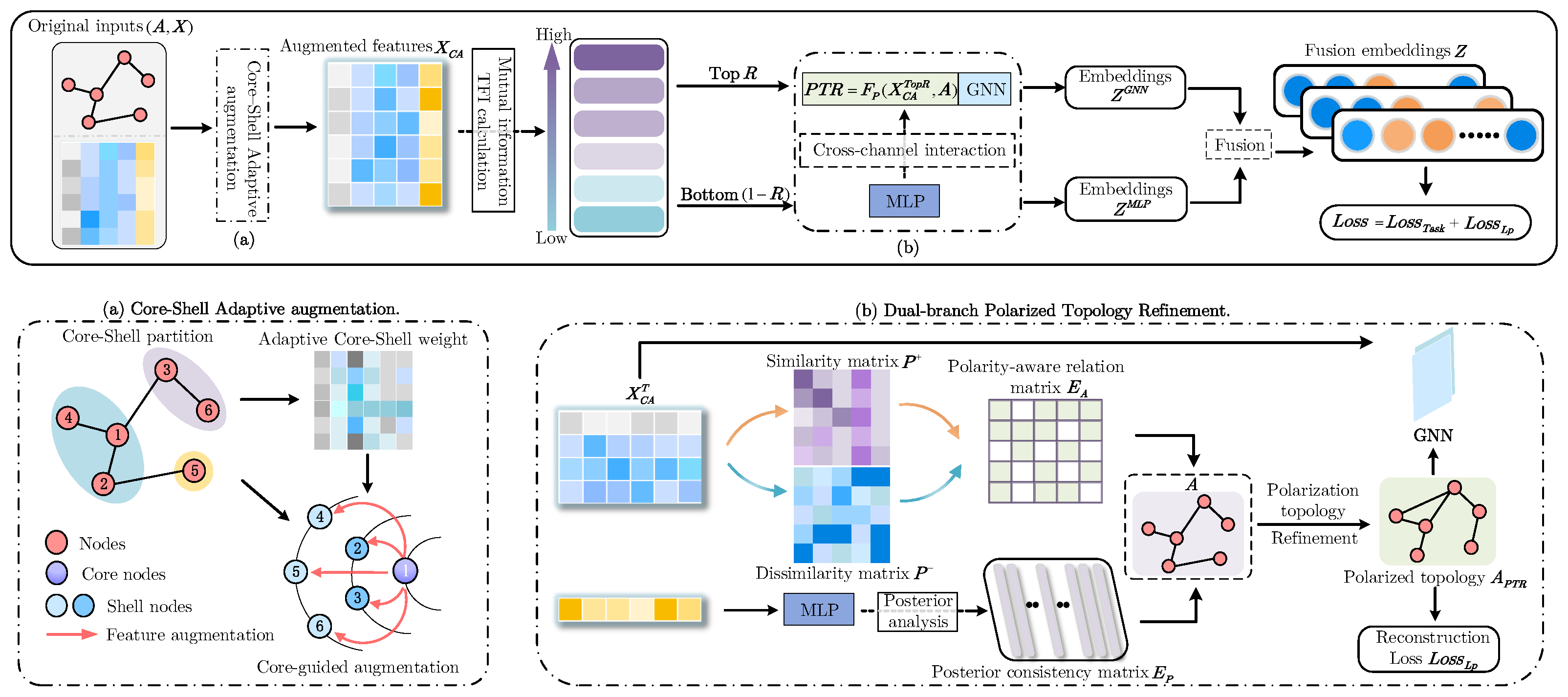
The overall architecture of CSA-PTR is illustrated in Figure 3. Our framework consists of the following modules:

(1)

Graph feature splitting: This module adopts the TFI-based feature-splitting strategy to estimate feature-wise propagation preference and divide the input features into a propagation-favored branch and a graph-agnostic branch.

(2)

Core–shell adaptive augmentation: This module is designed to alleviate the bias in propagation preference estimation caused by locally mixed neighborhoods. It leverages granular-ball-based local grouping to derive more reliable core–shell-aware support for node representations, thereby providing a better context for subsequent feature-wise preference estimation.

(3)

Dual-branch Polarized Topology Refinement: This module is developed to address the mismatch between the selected propagation features and the original topology. By learning complementary polarized relation patterns in a dual-branch manner, this module refines the topology used for message passing and enables more effective propagation.

Figure 3. Overview of the proposed CSA-PTR framework. Starting from the original graph $(A,X)$, the model first applies Core–shell adaptive augmentation (CSA), as shown in (a), to enhance node features with more reliable local support. It then performs TFI-based feature splitting to divide the features into a propagation-favored branch and a graph-agnostic branch. For the former, Dual-branch Polarized Topology Refinement (DPTR), as shown in (b), refines the propagation topology through polarity-aware relations and posterior consistency derived from the graph-agnostic branch. Finally, the two branches are encoded separately and fused for node classification.

Figure 3. Overview of the proposed CSA-PTR framework. Starting from the original graph $(A,X)$, the model first applies Core–shell adaptive augmentation (CSA), as shown in (a), to enhance node features with more reliable local support. It then performs TFI-based feature splitting to divide the features into a propagation-favored branch and a graph-agnostic branch. For the former, Dual-branch Polarized Topology Refinement (DPTR), as shown in (b), refines the propagation topology through polarity-aware relations and posterior consistency derived from the graph-agnostic branch. Finally, the two branches are encoded separately and fused for node classification.

3.3. Graph Feature Splitting (GFS)

Following the feature-splitting paradigm introduced in TFI, we first divide the input feature dimensions into a graph-favored part and a graph-disfavored part. The intuition is that graph propagation is not uniformly beneficial to all feature dimensions. Some dimensions are more compatible with topology-aware aggregation and can benefit from message passing, whereas others may be degraded by neighborhood mixing and are therefore better handled by a graph-agnostic encoder. Based on this observation, GFS routes different feature dimensions to different learning branches instead of applying the same propagation operator to the entire feature space.

Existing graph metrics mainly characterize feature similarity over connected nodes. However, for feature splitting, what we need to evaluate is not merely whether neighboring nodes are similar, but whether graph propagation on a specific feature dimension can provide label-relevant information for downstream prediction. To this end, mutual information offers a suitable tool, as it directly measures the statistical dependence between variables and can capture both linear and non-linear relationships [31].

To measure the propagation preference of each feature dimension, TFI assigns the d-th feature dimension a topology-aware informativeness score:

$${\mathrm{TFI}}_d=I\left(y;{\tilde{\mathbf{X}}}_{:,d}\right),$$

(1)

where ${\tilde{\mathbf{X}}}_{:,d}={\tilde{\mathbf{A}}}^k{\mathbf{X}}_{:,d}$ denotes the propagated signal of the d-th feature dimension, k is the propagation hop, and y denotes the node label random variable. A larger ${\mathrm{TFI}}_d$ indicates that the d-th feature dimension contains more label-relevant information after graph propagation, and is therefore more suitable for topology-aware encoding.

Specifically, the mutual information term in Equation (1) is computed as

$$I(U;V)=\sum _{v\in \mathcal{V}}\sum _{u\in \mathcal{U}}p(u,v)\log {\displaystyle \frac{p(u,v)}{p\left(u\right)p\left(v\right)}},$$

(2)

where U and V denote two random variables, $p(u,v)$ is their joint probability distribution, and $p\left(u\right)$ and $p\left(v\right)$ are the corresponding marginal probability distributions. In Equation (1), U and V correspond to the label variable y and the propagated feature signal ${\tilde{\mathbf{X}}}_{:,d}$, respectively.

In practice, TFI is estimated on the labeled training nodes only, so that no supervision from validation or test nodes is involved in feature splitting. For each feature dimension, the aggregated scalar signal is discretized into B bins by quantile-based partitioning, and the mutual information is then computed from the empirical joint distribution between the discretized signal and labels. To avoid excessive computational overhead and training instability, the feature split is computed before the main optimization stage and kept fixed during training unless otherwise specified.

After computing ${\mathrm{TFI}}_d$ for all feature dimensions, we rank these scores and split the feature space according to a ratio $r\in (0,1)$. Let ${\tau }_r$ be the threshold for selecting the top-r fraction of feature dimensions according to their TFI scores. The graph-favored feature subset ${\mathbf{X}}^G$ and the graph-disfavored feature subset ${\mathbf{X}}^M$ are defined as follows:

$$\begin{array}{cc}\hfill {\mathbf{X}}^G& =\{{\mathbf{X}}_{:,d}\mid {\mathrm{TFI}}_d\ge {\tau }_r\},\hfill \\ \hfill {\mathbf{X}}^M& =\{{\mathbf{X}}_{:,d}\mid {\mathrm{TFI}}_d<{\tau }_r\}.\hfill \end{array}$$

(3)

In this way, the original feature matrix is decomposed into a propagation-oriented part and a non-propagation part.

The two subsets are then processed by separate encoders. Specifically, the graph-favored features ${\mathbf{X}}^G$ are fed into a GNN branch to exploit informative neighborhood interactions, while the graph-disfavored features ${\mathbf{X}}^M$ are processed by an MLP branch to preserve discriminative signals without introducing unnecessary message mixing. For the ℓ-th layer, the two branches are written as

$$\begin{array}{cc}\hfill {\mathbf{H}}_G^{(\ell )}& =\sigma \left(\tilde{\mathbf{A}}{\mathbf{H}}_G^{(\ell -1)}{\mathbf{W}}_G^{(\ell -1)}\right),\hfill \\ \hfill {\mathbf{H}}_M^{(\ell )}& =\sigma \left({\mathbf{H}}_M^{(\ell -1)}{\mathbf{W}}_M^{(\ell -1)}\right),\hfill \end{array}$$

(4)

where ${\mathbf{H}}_G^{\left(0\right)}={\mathbf{X}}^G$ and ${\mathbf{H}}_M^{\left(0\right)}={\mathbf{X}}^M$.

Finally, the outputs of the two branches are fused to obtain the final node representation:

$$\mathbf{Z}=\left[{\mathbf{H}}_G^{\left(L\right)}\parallel {\mathbf{H}}_M^{\left(L\right)}\right]{\mathbf{W}}_f+{\mathbf{b}}_f,$$

(5)

where $[·\parallel ·]$ denotes concatenation, and ${\mathbf{W}}_f$ and ${\mathbf{b}}_f$ are trainable parameters. The fused representation $\mathbf{Z}$ is then used for downstream node classification. Through this split-processing design, GFS provides an explicit implementation of selective propagation at the feature-dimension level.

3.4. Core–Shell Adaptive Augmentation (CSA)

Although GFS determines feature-wise propagation preference through a statistical criterion, the reliability of this estimation still depends on the local context from which the aggregated signals are formed. In realistic graphs, however, local neighborhoods are often mixed and structurally unstable: nodes near class boundaries may be surrounded by label-inconsistent neighbors, making the resulting context less reliable for judging whether a feature dimension should be propagated. Therefore, the role of CSA is to construct a cleaner contextual space for more reliable TFI estimation before feature splitting.

To examine how different context construction strategies affect TFI estimation, we conduct an exploratory comparison of six variants, including perturbation-based, masking-based, and clustering-based methods. As shown in

Table 1. Comparison of different context enhancement strategies on TFI-related statistics across three citation datasets. “Top K%” denotes the average TFI over the top-K% feature dimensions ranked by TFI. Bold: best.

Datasets	Metrics	Methods
		Default	Gauss	Shuffle	Dim_masked	Entry_masked	Cluster
Cora	Mean	0.0306	0.0321	0.0259	0.0274	0.0295	0.0331
	Top 5%	0.1609	0.1414	0.1354	0.1507	0.1588	0.1692
	Top 10%	0.1335	0.1230	0.1146	0.1235	0.1318	0.1411
	Top 20%	0.1034	0.0996	0.0952	0.0952	0.1031	0.1102
Citeseer	Mean	0.0261	0.0245	0.0241	0.0237	0.0244	0.0270
	Top 5%	0.1388	0.1354	0.1376	0.1338	0.1351	0.1447
	Top 10%	0.1163	0.1138	0.1136	0.1118	0.1136	0.1218
	Top 20%	0.0920	0.0891	0.0878	0.0870	0.0891	0.0958
Pubmed	Mean	0.0393	0.0406	0.0268	0.0370	0.0327	0.0416
	Top 5%	0.2054	0.1987	0.1470	0.1831	0.2586	0.2087
	Top 10%	0.1713	0.1703	0.1240	0.1521	0.1630	0.1723
	Top 20%	0.1325	0.1353	0.0982	0.1222	0.1101	0.1365

, the clustering-based variant yields the most consistent improvement across datasets. This result suggests that effective TFI estimation benefits more from a cleaner contextual space for aggregation than from generic structure-agnostic perturbations. One possible explanation is that clustering-based augmentation reorganizes nodes with similar characteristics into compact local groups, thereby reducing the interference caused by mixed boundary neighborhoods and providing cleaner contextual support for propagation preference estimation.

This intuition can also be understood from the formulation of TFI. Using the identity of mutual information, we have

$${\mathrm{TFI}}_d=H\left(y\right)-H\left(y\mid {\tilde{\mathbf{X}}}_{:,d}\right),$$

(6)

where $H\left(y\right)$ is fixed for a given dataset. Therefore, improving ${\mathrm{TFI}}_d$ is equivalent to reducing the conditional uncertainty $H\left(y\mid {\tilde{\mathbf{X}}}_{:,d}\right)$. In mixed boundary neighborhoods, semantically inconsistent neighbors may participate in aggregation, making the resulting aggregated signal less discriminative for predicting labels and thus increasing the conditional uncertainty. By contrast, a cleaner contextual space can provide more stable local evidence, making the aggregated feature more informative about the label distribution. More specifically, boundary nodes distort TFI estimation by perturbing the empirical dependency between the propagated feature signal and the label variable. When label-inconsistent neighbors are mixed during propagation, similar propagated feature values may no longer provide stable label-discriminative cues. Consequently, the empirical label uncertainty conditioned on the same discretized feature bin increases, which enlarges $H\left(y\mid {\tilde{\mathbf{X}}}_{:,d}\right)$ and lowers ${\mathrm{TFI}}_d$. As a result, some potentially graph-favored dimensions may be underestimated and incorrectly assigned to the graph-agnostic branch, leading to biased feature splitting.

These observations further suggest that the choice of context constructor is also critical. For TFI estimation, a suitable constructor should preserve local purity and structural stability, thereby providing more reliable contextual support for feature-wise propagation preference estimation. Prior studies suggest that effective aggregation relies on stable intra-class topological patterns rather than consistency-based metrics alone [32]. From this perspective, granular computing provides a suitable inductive principle, as it organizes samples into compact information granules that better capture locally coherent and semantically stable regions [33]. In particular, the purity-skeleton dynamic hypergraph suggests that a purity-aware, granular-ball construction can effectively organize feature-space correlations and data distributions into structured local regions [34], thereby preserving important information and providing a more reliable contextual basis for TFI estimation.

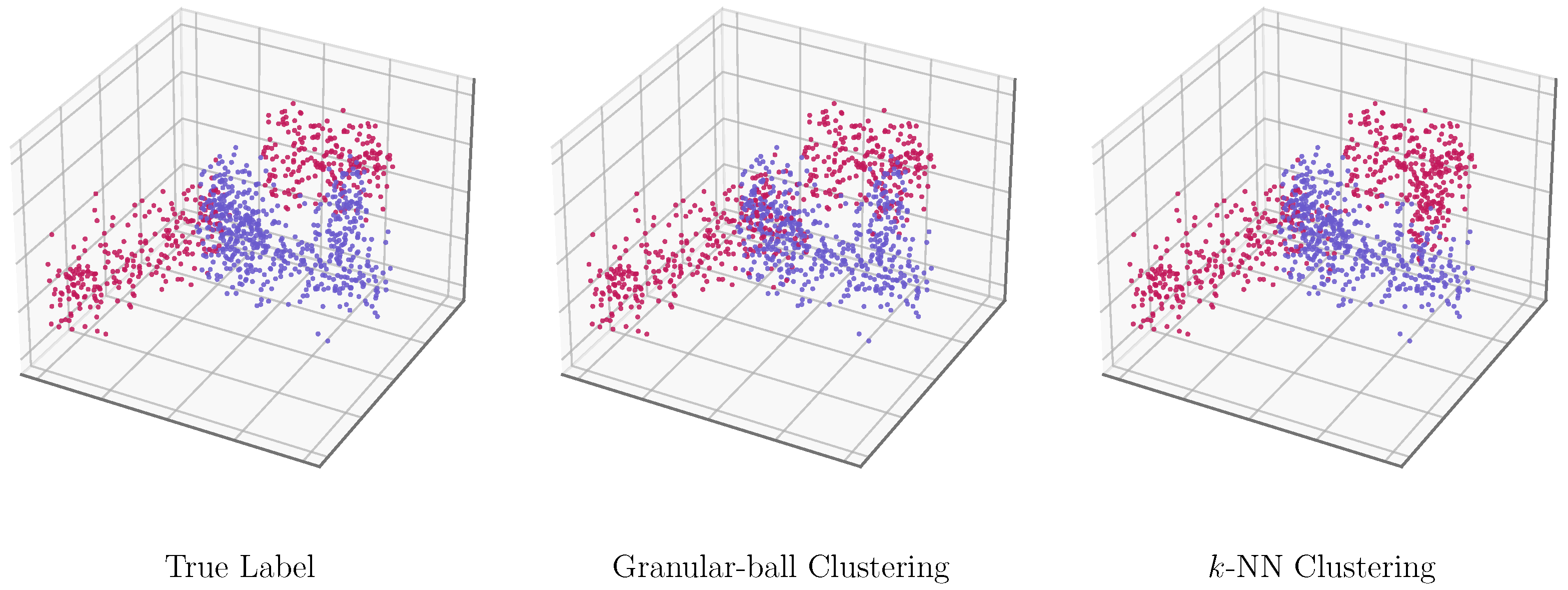
As further illustrated in Figure 4, granular-ball clustering yields cleaner local partitions than k-NN clustering, especially around boundary regions, which is consistent with our goal of constructing a more reliable contextual space for TFI estimation. To further quantify this observation, we compute the partition purity on a sampled class-pair subgraph from the dataset. For each granular ball $B_m$, its purity is defined as $P\left(B_m\right)={\max }_c|v_i\in B_m=c|/|B_m|$, and the weighted granular-ball purity is computed as ${\overline{P}}_{GB}={\sum }_m|B_m|P\left(B_m\right)/N_s$, where $N_s$ is the number of nodes in the sampled subgraph. For k-NN, since it does not produce explicit disjoint clusters, we treat each node’s k-nearest-neighbor set $\mathcal{N}k\left(i\right)$ as its local context and compute the average local purity as $\overline{P}kNN=N_s^{-1}{\sum }_i{\max }_c|v_j\in {\mathcal{N}}_k\left(i\right)=c|/|{\mathcal{N}}_k\left(i\right)|$.

As shown in

Table 2. Partition purity comparison between granular-ball clustering and k-NN clustering.

Region	Granular-Ball	k-NN	Relative Improvement (%)
Whole graph	0.8200	0.8102	1.21
Boundary region	0.7962	0.7333	8.58

, granular-ball clustering achieves slightly higher purity on the whole subgraph and a much larger improvement in the boundary region. In particular, the relative improvement reaches 8.58% in the boundary region, indicating that its advantage mainly lies in suppressing label mixing near class boundaries. This quantitative result supports the visual observation in Figure 4: k-NN may connect feature-close but label-inconsistent nodes around boundary regions, whereas purity-aware, granular-ball clustering can recursively separate low-purity regions and form cleaner local contexts. Therefore, what we need is a purity-aware context constructor that can suppress boundary contamination while preserving structurally stable local support for TFI estimation. Motivated by this observation, we design CSA to instantiate such a context enhancement mechanism.

Specifically, CSA constructs a contextual space composed of two complementary parts: a purity-aware core and an anchor-guided shell. The design choice is intentionally lightweight in function rather than exhaustive in mechanism: the core is introduced to suppress local boundary contamination, while the shell is introduced only to provide complementary structural support when local evidence is insufficient.

We first use a clustering algorithm to partition the node feature space into a set of local granular balls $\mathcal{B}=\{B_1,\dots ,B_M\}$. For each ball $B_m$, its center and radius are defined as

$${\mathbf{c}}_m={\displaystyle \frac{1}{|B_m|}}\sum _{{\mathbf{x}}_i\in B_m}{\mathbf{x}}_i,$$

(7)

$$r_m={\displaystyle \frac{1}{|B_m|}}\sum _{{\mathbf{x}}_i\in B_m}\parallel {\mathbf{x}}_i-{\mathbf{c}}_m\parallel ,$$

(8)

where ${\mathbf{x}}_i$ denotes the feature vector of node $v_i$, and the summation is taken over all nodes whose feature vectors belong to the granular ball $B_m$.

Following the granular ball computing formulation, the purity of $B_m$ is measured as

$$\mathrm{purity}\left(B_m\right)={\displaystyle \frac{{\max }_{1\le t\le K_m}|{\mathcal{S}}_t\left(B_m\right)|}{{\sum }_{t=1}^{K_m}|{\mathcal{S}}_t\left(B_m\right)|}},$$

(9)

where ${\mathcal{S}}_t\left(B_m\right)$ denotes the subset of samples in the t-th subcluster of $B_m$, and $K_m$ is the number of subclusters in $B_m$. Balls with purity lower than a hyperparameter threshold p are recursively split until the criterion is satisfied. In this way, the resulting purity-ball set provides compact local regions that better reflect the feature-space distribution and reduce boundary-induced mixing.

For each node $v_i$, let $q\left(i\right)$ denote the index of the granular ball containing it. We then define the core representation of $v_i$ as

$${\mathbf{h}}_i^{\mathrm{core}}=(1-\lambda ){\mathbf{x}}_i+\lambda {\mathbf{c}}_{q\left(i\right)},$$

(10)

where $\lambda \in [0, 1]$ controls the strength of local purity-aware refinement.

While the core improves local semantic coherence, TFI estimation also benefits from complementary structural evidence beyond a single granular ball. To this end, we select a small set of representative anchor nodes from the largest granular balls. Let $\mathcal{A}=\{a_1,\dots ,a_S\}$ denote the anchor set, where each anchor is chosen as the highest-degree node in one selected large ball:

$$a_s=\arg \underset{v_j\in B_{\left(s\right)}}{\max }\mathrm{deg}\left(v_j\right),$$

(11)

with $B_{\left(s\right)}$ denoting the s-th selected large granular ball.

To make the shell aware of granular-ball boundaries under purity-aware guidance, we define a purity-aware, ball-level edge cost ${\omega }_{uv}$ and compute the shortest ball-aware distance $d_{\mathcal{B}}(i,a_s)$ from node $v_i$ to anchor $a_s$:

$${\omega }_{uv}=\left\{\begin{array}{cc}{\omega }_{\mathrm{in}},\hfill & q\left(u\right)=q\left(v\right),\hfill \\ {\omega }_{\mathrm{out}},\hfill & q\left(u\right)\ne q\left(v\right),\hfill \end{array}\right.{\omega }_{\mathrm{out}}>{\omega }_{\mathrm{in}}>0,$$

(12)

$$d_{\mathcal{B}}(i,a_s)=\underset{\pi :i⇝a_s}{\min }\sum _{(u,v)\in \pi }{\omega }_{uv}.$$

(13)

For subsequent computation, we further map this distance into an anchor affinity ${\alpha }_{is}$ and use these affinities to obtain the shell representation of node $v_i$:

$${\alpha }_{is}=\sigma \left(-d_{\mathcal{B}}(i,a_s)\right),$$

(14)

$${\mathbf{h}}_i^{\mathrm{shell}}={\displaystyle \frac{{\sum }_{s=1}^S{\alpha }_{is}{\mathbf{x}}_{a_s}}{{\sum }_{s=1}^S{\alpha }_{is}+\epsilon }},$$

(15)

where $\sigma (·)$ is the sigmoid function and $\epsilon$ is a small constant.

However, the need for shell supplementation is not uniform across nodes. Nodes located in locally stable regions usually already possess sufficiently reliable contextual support and, therefore, require only limited shell enhancement, whereas nodes near boundary regions are more likely to suffer from unstable local evidence and thus need stronger structural compensation. This suggests that the amount of injected shell information should be adjusted according to each node’s structural role. Inspired by the idea of local-global centrality, which jointly characterizes nodes from local and global structural perspectives, we introduce a node-wise adaptive weight to modulate the strength of shell information injected into each node [35]. Specifically, we quantify each node from two complementary aspects, namely local influence ($\mathrm{LI}$) and global influence ($\mathrm{GI}$), which are defined as follows:

$$\begin{array}{cc}\hfill {\mathrm{LI}}_i& ={\displaystyle \frac{\mathrm{deg}\left(v_i\right)}{{\max }_{v_j\in \mathcal{V}}\mathrm{deg}\left(v_j\right)}},\hfill \\ \hfill {\mathrm{GI}}_i& ={\displaystyle \sum _{s=1}^S}{\alpha }_{is}\sqrt{\mathrm{deg}\left(a_s\right)}.\hfill \end{array}$$

(16)

We further combine them into an adaptive centrality score

$${\mathrm{LGC}}_i={\mathrm{LI}}_i\left({\mathrm{GI}}_i+\gamma {\displaystyle \sum _{s=1}^S}{\alpha }_{is}\right),$$

(17)

where $\gamma$ is a balancing coefficient. After min-max normalization, the node-wise fusion weight is obtained as

$$w_i={\displaystyle \frac{{\mathrm{LGC}}_i-{\min }_j{\mathrm{LGC}}_j}{{\max }_j{\mathrm{LGC}}_j-{\min }_j{\mathrm{LGC}}_j+\epsilon }}.$$

(18)

Finally, we combine the core and shell to obtain final feature ${\mathbf{X}}^{\mathrm{CSA}}$ and estimate TFI on the CSA-enhanced context.

$${\mathbf{x}}_i^{\mathrm{CA}}={\mathbf{h}}_i^{\mathrm{core}}+w_i{\mathbf{h}}_i^{\mathrm{shell}}.$$

(19)

$${\tilde{\mathbf{X}}}_{:,d}^{\mathrm{CA}}={\tilde{\mathbf{A}}}^k{\mathbf{X}}_{:,d}^{\mathrm{CA}}.$$

(20)

$${\mathrm{TFI}}_d^{\mathrm{CA}}=I\left(y;{\tilde{\mathbf{X}}}_{:,d}^{\mathrm{CA}}\right).$$

(21)

The purity-aware core reduces the ambiguity in feature-preference estimation, while the adaptive shell provides a more reliable structural context. In this way, CSA stabilizes node representations to support clearer feature splitting.

In addition to improving the reliability of feature-preference estimation, CSA is designed as a lightweight preprocessing component, where the main extra cost comes from purity-aware, granular-ball clustering. Following the notation above, let $N=|\mathcal{V}|$ and F denote the number of nodes and the input feature dimension, respectively. Since the granular-ball set has been defined as $\mathcal{B}=B_1,\dots ,B_M$, M denotes the number of generated granular balls, while the number of graph edges is written explicitly as $|\mathcal{E}|$. Let I denote the maximum number of recursive splitting iterations in the purity-aware, granular-ball clustering process, and let S denote the number of selected anchors. Since CSA is conducted before TFI-based feature splitting, it introduces a one-time preprocessing cost rather than an additional cost repeatedly incurred in each training epoch.

Specifically, purity-aware, granular-ball clustering recursively checks and splits low-purity balls. In each splitting iteration, the algorithm scans node features in the current balls to compute ball centers, radii, and purity scores. Since all nodes are visited at most once in each iteration, this clustering step costs $O\left(INF\right)$. After the granular balls are obtained, constructing the core representation only requires a feature-level interpolation between each node and the center of its corresponding ball, with cost $O\left(NF\right)$. Anchor selection can be completed by computing node degrees and scanning candidate balls, resulting in $O(|\mathcal{E}|+N)$ time. For the anchor-guided shell, computing ball-aware distances from S anchors on the sparse graph costs $O\left(S\right(|\mathcal{E}|+N\left)\log N\right)$ with a standard shortest-path implementation, and aggregating anchor features for all nodes costs $O\left(NSF\right)$. The adaptive core–shell fusion further costs $O(NS+NF)$. Therefore, the overall time complexity of CSA is $O(INF+S(|\mathcal{E}|+N)\log N+NSF+|\mathcal{E}|)$.

The following dual-branch forward propagation after feature splitting also does not double the graph propagation cost. Let $F_G$ and $F_M$ denote the dimensions of the graph-favored and graph-agnostic feature subsets, respectively, where $F_G+F_M=F$. Only the graph-favored subset ${\mathbf{X}}^G\in {\mathbb{R}}^{N\times F_G}$ is fed into the GNN branch and involves sparse neighborhood aggregation, while the graph-agnostic subset ${\mathbf{X}}^M\in {\mathbb{R}}^{N\times F_M}$ is processed by an MLP branch without using the adjacency matrix. Therefore, the MLP branch introduces only node-wise feature transformation cost, e.g., $O\left(N{F}_{M}H\right)$ for a hidden dimension H, and does not incur edge-wise message passing cost such as $O(|\mathcal{E}|F_M)$. Since $F_G+F_M=F$, the dual-branch design reallocates features between graph-based and graph-agnostic encoders rather than applying two full graph propagations.

In our implementation, both I and S are bounded constants. Therefore, for sparse graphs where $|\mathcal{E}|=O\left(N\right)$, the CSA preprocessing complexity reduces to a near-linear cost, approximately $O(NF+N\log N)$. The space complexity mainly comes from storing the enhanced node features, granular-ball assignments, ball centers, sparse graph structure, and anchor affinities, requiring $O(NF+MF+|\mathcal{E}|+NS)$ space. Since $M\le N$ and S is fixed, the space complexity is bounded by $O(NF+|\mathcal{E}|)$. Thus, although CSA introduces purity-aware, granular-ball clustering and the subsequent model adopts dual-branch forward propagation, the framework does not introduce dense pairwise computation or duplicate full graph propagation, and its additional cost remains lightweight compared with standard sparse graph learning.

3.5. Dual-Branch Polarized Topology Refinement (DPTR)

Although GFS separates graph-favored and graph-disfavored feature dimensions for selective propagation, the graph-based branch may still suffer from a practical mismatch: once the split propagation-oriented features are no longer well aligned with the original graph, message passing on the unchanged topology may route information through incompatible edges. Meanwhile, the graph-based and feature-only branches provide naturally complementary views, but their interaction remains limited if they are optimized independently. To address these issues, we introduce a Dual-branch Polarized Topology Refinement (DPTR) module, which refines the propagation topology from a polarized perspective and further coordinates this refinement with graph-independent evidence from the feature-only branch.

Let ${\mathbf{X}}^G\in {\mathbb{R}}^{N\times F_G}$ and ${\mathbf{X}}^M\in {\mathbb{R}}^{N\times F_M}$ denote the propagation-favored features and the feature-only features obtained by GFS, respectively. Following the polarized formulation, we define the similarity matrix $M_{ij}^{+}$ and the dissimilarity matrix $M_{ij}^{-}$ as

$$\begin{array}{cc}\hfill M_{ij}^{+}& =A_{ij}·{\left({\left(\mathbf{H}\right)}_{i,:}{\parallel \left(\mathbf{H}\right)}_{j,:}\right)}^{\top }{\mathbf{W}}_{+},\hfill \\ \hfill M_{ij}^{-}& =A_{ij}·{\left|{\left(\mathbf{H}{\mathbf{W}}_{-}\right)}_{i,:}-{\left(\mathbf{H}{\mathbf{W}}_{-}\right)}_{j,:}\right|}^2,\hfill \end{array}$$

(22)

where $\mid \mid$ denotes vector concatenation, $\mathbf{H}={\mathbf{X}}^G$, and ${\mathbf{W}}_{+}$ and ${\mathbf{W}}_{-}$ are learnable parameters.

On the MLP branch, we first obtain the branch embedding and then compute the posterior prediction as follows:

$$\begin{array}{cc}\hfill {\mathbf{Z}}^M& =\mathrm{MLP}\left({\mathbf{X}}^M\right),\hfill \\ \hfill {\mathbf{O}}^M& ={\mathbf{Z}}^M{\mathbf{W}}_o^M,\hfill \\ \hfill {\mathbf{P}}^M& =\mathrm{softmax}\left({\mathbf{O}}^M\right),\hfill \end{array}$$

(23)

where ${\mathbf{W}}_o^M$ is the output projection matrix, and ${\left({\mathbf{P}}^M\right)}_{i,:}$ denotes the posterior vector of node $v_i$.

Since the feature-only branch does not rely on graph propagation, its posterior provides graph-independent semantic evidence that can serve as a complementary cue for topology refinement. In particular, we use the inner product between posterior distributions to measure the semantic consistency between two nodes [36,37], and define

$$R_{ij}={\left({\mathbf{P}}^M\right)}_{i,:}{\left({\mathbf{P}}^M\right)}_{j,:}^{\top }.$$

(24)

To obtain a sparse and stable coordination operator, we further normalize and sparsify $R_{ij}$:

$${\left({\mathbf{E}}_P\right)}_{ij}=\left\{\begin{array}{cc}{\displaystyle \frac{\exp \left(R_{ij}\right)}{{\displaystyle \sum _{k\in {\mathrm{TopK}}_K\left(i\right)}}\exp \left(R_{ik}\right)}},\hfill & j\in {\mathrm{TopK}}_K\left(i\right),\hfill \\ 0,\hfill & \mathrm{otherwise},\hfill \end{array}\right.$$

(25)

where ${\mathrm{TopK}}_K\left(i\right)$ denotes the set of the top-K nodes with the largest posterior consistency scores for node $v_i$.

Equation (25) serves as a posterior coordination operator for topology refinement. Specifically, $A_{ij}$ anchors the refinement to the observed graph structure, $\exp (M_{ij}^{+}-\alpha M_{ij}^{-})$ provides polarized support from the graph-favored branch, and ${\left({\mathbf{E}}_P\right)}_{ij}$ acts as a semantic gate derived from the feature-only branch. The Top-K sparsification further keeps the coordination local and prevents over-dense semantic connections.

We then use the posterior consistency operator to coordinate the polarized relation term when constructing the refined topology:

$${\left({\mathbf{E}}_A\right)}_{ij}=A_{ij}+{\left({\mathbf{E}}_P\right)}_{ij}·A_{ij}·\exp \left(M_{ij}^{+}-\alpha M_{ij}^{-}\right),$$

(26)

where $\alpha >0$ is a learnable parameter.

Accordingly, we take ${\mathbf{A}}_{PTR}={\mathbf{E}}_A$ and define the normalized propagation matrix as

$${\tilde{\mathbf{A}}}_{PTR}={\mathbf{D}}_{PTR}^{-\frac{1}{2}}({\mathbf{A}}_{PTR}+\mathbf{I}){\mathbf{D}}_{PTR}^{-\frac{1}{2}},$$

(27)

where ${\mathbf{D}}_{PTR}$ is the degree matrix of ${\mathbf{A}}_{PTR}+\mathbf{I}$.

The graph-based branch then performs message passing on the refined topology and ${\mathbf{H}}_G^{\left(0\right)}={\mathbf{X}}^G$:

$${\mathbf{H}}_G^{(\ell )}=\sigma \left({\tilde{\mathbf{A}}}_{PTR}{\mathbf{H}}_G^{(\ell -1)}{\mathbf{W}}_G^{(\ell -1)}\right).$$

(28)

Let ${\mathbf{Z}}^G={\mathbf{H}}_G^{\left(L\right)}$ denote the output embedding of the graph-based branch. We then fuse the two branch representations and make the final prediction:

$$\mathbf{Z}=\left[{\mathbf{Z}}^G\parallel {\mathbf{Z}}^M\right]{\mathbf{W}}_f+{\mathbf{b}}_f.$$

(29)

For node classification, the task loss is defined as

$${Loss}_{Task}=-\sum _{v_i\in {\mathcal{V}}_L}{\displaystyle \sum _{c=1}^C}{Y}_{ic}\log {\widehat{Y}}_{ic}.$$

(30)

To jointly regularize the polarized topology and the posterior consistency operator, we introduce an auxiliary topology-coordination loss defined as

$${Loss}_{Lp}=tr\left({\mathbf{E}}_A^{\top }\mathbf{L}{\mathbf{E}}_A\right)-\left(\sum _{(v_i,v_j)\in \mathcal{E}}\log R_{ij}+\sum _{(v_i,v_j)\in {\mathcal{E}}^{-}}\log \left(1-R_{ij}\right)\right),$$

(31)

where $\mathbf{L}=\mathbf{D}-\mathbf{A}$ is the Laplacian matrix of the original graph, ${\mathcal{E}}^{-}$ denotes a set of sampled non-edge pairs. The overall objective is $Loss={Loss}_{Task}+{Loss}_{Lp}.$

The first term regularizes the refined relation matrix with respect to the graph structure, encouraging structurally coherent topology refinement. The second term explicitly increases posterior agreement on observed edges while discouraging high agreement on sampled non-edge pairs. In this way, $Los{s}_{Lp}$ constrains the refined topology from both structural and semantic perspectives.

The complexity of DPTR mainly comes from the pairwise polarized topology refinement. Let $F_G$ and $F_M$ denote the dimensions of the graph-favored and graph-agnostic feature subsets, respectively, where $F_G+F_M=F$. Let H denote the hidden dimension, C denote the number of classes, L denote the number of GNN layers, and K denote the number of retained posterior-consistency neighbors. Different from the CSA module, DPTR is performed during model training. Following the polarized topology perturbation formulation, the similarity matrix $M^{+}$ and the dissimilarity matrix $M^{-}$ are defined over node pairs. Therefore, computing the pairwise polarized relation introduces a quadratic term with respect to the number of nodes.

Specifically, projecting the graph-favored features ${\mathbf{X}}^G$ into the hidden space costs $O\left(N{F}_{G}H\right)$. Computing the pairwise similarity and dissimilarity scores over node pairs costs $O\left(N^{2}H\right)$, and storing the corresponding polarized relation matrices requires $O\left(N^2\right)$ space before sparsification. On the graph-agnostic branch, the MLP produces posterior predictions through node-wise transformations, with cost $O(N{F}_{M}H+NHC)$. The posterior consistency matrix R is computed by pairwise inner products between posterior distributions, which costs $O\left(N^{2}C\right)$ time and requires $O\left(N^2\right)$ temporary storage if fully materialized. The subsequent Top-K operation sparsifies the posterior coordination operator and keeps only K candidates for each node, leading to a sparse operator with $O\left(NK\right)$ stored entries.

After the polarized relation and posterior coordination are obtained, the refined topology is constructed by coordinating the original adjacency, polarized relation scores, and posterior consistency. The final message passing is performed on the refined topology. If the refined topology is stored after Top-K sparsification and adjacency-based masking, the propagation cost is $O(L|\mathcal{E}\ast PTR|H)$, where $|\mathcal{E}\ast PTR|$ denotes the number of retained edges in the refined topology. Therefore, the per-epoch time complexity of DPTR can be summarized as $O(N{F}_{G}H+N{F}_{M}H+NHC+N^{2}H+N^{2}C+L|\mathcal{E}\ast PTR|H)$, and its additional space complexity is $O(NH+NC+N^2+|\mathcal{E}\ast PTR|)$.

Although DPTR introduces a quadratic pairwise relation-estimation term, this cost is controlled in two aspects. First, the polarized computation is applied to the graph-favored branch after feature splitting, rather than to the entire original feature space. Second, the graph-agnostic branch is implemented by an MLP and does not introduce another graph propagation process. Moreover, Top-K sparsification prevents the refined topology used for message passing from becoming fully dense. Therefore, DPTR introduces additional pairwise topology-refinement overhead, but it does not duplicate full graph convolution over both branches. This design provides a practical trade-off between topology refinement capability and computational cost on the evaluated benchmark graphs.

In this way, DPTR first learns polarity-aware relations directly from the split propagation-favored features, and then further uses posterior consistency from the feature-only branch as complementary guidance to coordinate topology refinement. The resulting topology is better aligned with the split propagation features, thereby alleviating feature–topology mismatch and reducing the risk that messages are passed along incompatible edges. For clarity, we summarize the overall procedure of CSA-PTR in Algorithm 1.

Algorithm 1 The overall procedure of CSA-PTR.

Require: Graph adjacency matrix $\mathbf{A}$, feature matrix $\mathbf{X}$, labels $\mathbf{Y}$, maximal training epochs T Ensure: Prediction result $\widehat{\mathbf{Y}}$   1: Initialize model parameters   2: Construct context-enhanced features ${\mathbf{X}}^{\mathrm{CA}}$ via Equation (21)   3: Compute TFI scores on ${\mathbf{X}}^{\mathrm{CA}}$ and split features ${\mathbf{X}}^{\mathrm{CA}}$ into ${\mathbf{X}}^G$ and ${\mathbf{X}}^M$   4: for $epoch=1,2,\dots ,T$ do   5:       Construct polarized relations based on ${\mathbf{X}}^G$ via Equation (22)   6:       Obtain posterior consistency operator ${\mathbf{E}}^P$ from the MLP branch on ${\mathbf{X}}^M$ via Equation (25)   7:       Construct refined topology ${\mathbf{A}}^{\mathrm{PTR}}$ via Equation (26)   8:       Obtain graph-based embedding ${\mathbf{Z}}^G$ with GNN on ${\mathbf{X}}^G$ and ${\mathbf{A}}^{\mathrm{PTR}}$   9:       Obtain feature-only embedding ${\mathbf{Z}}^M$ with MLP on ${\mathbf{X}}^M$ 10:       Fuse ${\mathbf{Z}}^G$ and ${\mathbf{Z}}^M$ to obtain $\widehat{\mathbf{Y}}$ via Equation (29) 11:       Compute the $Loss$ 12:       Update parameters by gradient descent 13: end for 14: return $\widehat{\mathbf{Y}}$

4. Experiments

In this section, we evaluate the proposed CSA-PTR against several state-of-the-art graph-based semi-supervised node classification methods, followed by ablation studies to examine the contributions of its key components.

4.1. Experiment Setup

4.1.1. Datasets

We adopt seven benchmark datasets to evaluate the effectiveness of the proposed method. The datasets are summarized in

Table 3. Data details.

Datasets	Nodes	Edges	Features	Classes
Cora	2708	5429	1433	7
Citeseer	3327	4732	3703	6
Pubmed	19,717	44,338	500	3
Actor	7600	26,659	932	5
Texas	183	325	1703	5
Cornell	183	295	1703	5
Wisconsin	251	499	1703	5

, which are briefly introduced as follows. Cora, Citeseer, and Pubmed are three widely used citation networks, where nodes represent scientific publications and edges denote citation links; Actor is an actor co-occurrence network, where nodes correspond to actors and edges indicate co-occurrence relationships on the same Wikipedia page; Texas, Cornell, and Wisconsin are three WebKB webpage networks, where nodes represent webpages and edges correspond to hyperlinks between webpages [38].

4.1.2. Baselines

We compare CSA-PTR with state-of-the-art models under the same label rate settings. (1) Classical GNNs: GCN [19], GAT [20], GraphSAGE [39], SGC [40]. (2) Mutual information-based methods: DGI [41], GFS-GCN [15]. (3) High-order modeling approaches: MOGCN [42]. (4) granular-ball-based methods: PS-DHGNN [34], PGBSF-GCN [43]. (5) polarization-based models: PMP-GNN [28]. (6) Advanced methods: PAGCN [44], LoGo-GNN [45], JNSGSL [46].

4.1.3. Implementation Details

All experiments are conducted on a computer equipped with an NVIDIA RTX 4070 GPU. Our model is implemented in Python 3.10 with PyTorch 2.4.0. To better evaluate the proposed CSA-PTR on semi-supervised node classification tasks, we conduct experiments on seven benchmark datasets under the settings described above. Unless otherwise specified, we use a hidden dimension of 32, set the learning rate to 0.005, set the weight decay to 0.001, set the anchor number to 5, fix the dropout rate to 0.6, and set the propagation hop k to 2. For the auxiliary hyperparameters in CSA and DPTR, we set the core interpolation strength $\lambda$ to 0.05, the LGC balance coefficient $\gamma$ to 0.2, and the number of Top-K posterior candidates K to 10. For all experiments, node classification accuracy (ACC) is adopted as the evaluation metric. Our method is run multiple times under random initialization, and the average results are reported. For baseline methods, we use the results reported in the corresponding papers.

4.2. Experimental Results

Table 4. ACC (%) of node classification tasks. Bold: best; underline: second-best.

Methods	Datasets
	Cora	Citeseer	Pubmed	Actor	Texas	Cornell	Wisconsin
GCN	81.5	69.5	79.2	27.9	62.1	37.8	45.8
GAT	83.0	72.6	79.0	27.8	59.4	43.2	49.4
GraphSAGE	82.4	71.9	79.4	26.3	50.6	40.5	49.2
SGC	81.0	71.9	78.9	27.1	51.3	43.2	52.9
DGI	82.3	71.8	76.8	28.2	64.8	45.9	54.9
MOGCN	83.3	72.4	79.2	25.4	54.0	45.9	54.9
PS-DHGNN	82.3	69.9	80.3	32.7	67.5	64.8	52.9
PGBSF-GCN	80.4	70.7	81.6	27.1	37.5	50.0	45.7
PMP-GNN	84.1	72.7	82.3	33.5	59.4	56.7	60.7
PAGCN	83.6	70.4	79.3	28.5	60.2	41.2	56.9
LoGo-GNN	84.6	73.4	81.6	31.2	67.6	45.9	52.9
GFS-GCN	81.7	71.6	81.8	33.2	72.9	68.1	72.5
JNSGSL	83.2	74.1	79.6	28.2	64.8	56.7	56.8
Ours	84.7	72.9	82.9	35.4	75.6	72.9	76.4

presents the node classification accuracy of CSA-PTR and various baseline methods on seven benchmark datasets, where ours denotes the performance of CSA-PTR. Overall, CSA-PTR achieves competitive and often superior performance across the evaluated datasets. In particular, it attains the best results on several benchmarks while remaining competitive on the others. These observations suggest that improving both the reliability of feature-wise preference estimation and the suitability of post-splitting propagation paths can be beneficial in practice.

To further evaluate the performance of CSA-PTR under different supervision levels, we conduct experiments with varying numbers of labeled nodes per class, as shown in Table 5. Specifically, for Cora and Citeseer, we use {4, 8, 12, 16, 20} labeled nodes per class, while for Pubmed, we use {5, 9, 12, 15, 20} labeled nodes per class, and we observe the following results:

(1)

Across different label settings, CSA-PTR maintains competitive and generally stable performance on all three datasets. This suggests that the proposed framework is not overly sensitive to the amount of supervision under the evaluated settings.

(2)

The advantage of CSA-PTR is particularly evident on Pubmed. In terms of average classification accuracy, CSA-PTR surpasses the second-best method by 2.5% and achieves the best result across all considered label settings. This trend is broadly consistent with our motivation: under limited supervision, propagation preference estimation becomes more vulnerable to locally mixed neighborhoods, while CSA and DPTR jointly improve the reliability of splitting and the suitability of propagation paths.

(3)

On Citeseer, CSA-PTR is slightly inferior to JNSGSL in the main comparison, but the label-rate results provide a more nuanced observation. Under lower supervision levels, CSA-PTR outperforms JNSGSL and achieves a higher average accuracy on Citeseer. This behavior is closely related to the characteristics of Citeseer, which has a relatively high-dimensional sparse feature space and a sparse citation topology, making model performance more sensitive to the amount of labeled data. With relatively sufficient supervision, JNSGSL can benefit from explicit graph structure learning and may introduce useful additional neighborhood relations beyond the observed sparse links. In contrast, when labeled nodes are limited, such learned structures may become less stable, while CSA-PTR relies on a more constrained selective propagation pipeline that improves the contextual basis for feature-wise preference estimation and refines the post-splitting propagation topology. This explains why CSA-PTR shows clearer advantages under low-label settings on Citeseer, while still remaining competitive in the main comparison.

Table 5. ACC (%) of node classification under different label rates. Bold: best; underline: second-best.

Datasets	Train	GCN	GAT	SGC	MOGCN	JNSGSL	PS-DHGNN	PGBSF-GCN	PMP-GNN	PAGCN	LoGo-GNN	GFS-GCN	Ours
Cora	28	62.3	66.8	57.6	71.5	69.4	58.0	58.6	61.0	65.8	68.6	58.1	63.2
	56	73.6	76.4	66.3	74.4	75.6	69.9	64.9	76.1	74.9	77.8	75.4	79.0
	84	76.7	77.9	74.3	77.2	79.0	74.8	69.7	77.5	77.1	80.7	76.3	80.0
	112	78.6	81.4	76.5	80.2	79.6	78.3	79.2	81.1	81.8	81.9	79.3	82.6
	140	81.5	82.2	81.0	82.4	83.2	82.3	80.4	84.1	83.6	84.6	81.7	84.7
	Average	74.5	76.9	71.1	77.1	77.4	72.7	70.6	76.0	76.6	78.7	74.2	77.9
Citeseer	24	55.7	55.6	43.9	55.2	58.9	53.6	54.9	59.4	53.7	55.6	51.8	60.2
	48	63.3	62.3	52.3	64.0	63.6	58.8	63.8	64.3	66.4	59.1	60.5	66.5
	72	65.8	66.3	59.6	66.1	68.6	63.1	67.1	67.2	65.8	60.0	67.3	68.9
	96	67.1	67.8	63.0	69.0	72.2	64.1	69.8	69.4	68.7	70.1	68.7	71.6
	120	69.5	72.6	71.9	72.4	74.1	69.9	70.7	72.7	70.4	73.4	71.6	72.9
	Average	64.3	64.9	58.1	65.3	67.5	61.9	65.3	66.6	65.0	63.6	64.0	68.0
Pubmed	9	60.6	58.8	60.1	58.6	60.1	60.7	48.5	62.6	49.8	54.2	60.9	63.5
	15	58.2	52.3	56.5	62.3	57.5	66.5	56.5	61.9	65.1	59.2	61.7	66.9
	30	62.4	69.6	64.9	70.2	62.6	69.1	74.4	71.8	75.2	66.1	72.9	77.2
	45	77.6	77.1	77.0	77.1	77.5	72.4	77.8	79.7	76.1	69.2	79.7	80.3
	60	79.2	79.0	78.9	79.2	79.6	80.3	81.6	82.3	79.3	81.6	81.8	82.9
	Average	67.6	67.4	67.5	69.5	67.5	69.8	67.8	71.7	69.1	66.1	71.4	74.2

Table 5. ACC (%) of node classification under different label rates. Bold: best; underline: second-best.

Datasets	Train	GCN	GAT	SGC	MOGCN	JNSGSL	PS-DHGNN	PGBSF-GCN	PMP-GNN	PAGCN	LoGo-GNN	GFS-GCN	Ours
Cora	28	62.3	66.8	57.6	71.5	69.4	58.0	58.6	61.0	65.8	68.6	58.1	63.2
	56	73.6	76.4	66.3	74.4	75.6	69.9	64.9	76.1	74.9	77.8	75.4	79.0
	84	76.7	77.9	74.3	77.2	79.0	74.8	69.7	77.5	77.1	80.7	76.3	80.0
	112	78.6	81.4	76.5	80.2	79.6	78.3	79.2	81.1	81.8	81.9	79.3	82.6
	140	81.5	82.2	81.0	82.4	83.2	82.3	80.4	84.1	83.6	84.6	81.7	84.7
	Average	74.5	76.9	71.1	77.1	77.4	72.7	70.6	76.0	76.6	78.7	74.2	77.9
Citeseer	24	55.7	55.6	43.9	55.2	58.9	53.6	54.9	59.4	53.7	55.6	51.8	60.2
	48	63.3	62.3	52.3	64.0	63.6	58.8	63.8	64.3	66.4	59.1	60.5	66.5
	72	65.8	66.3	59.6	66.1	68.6	63.1	67.1	67.2	65.8	60.0	67.3	68.9
	96	67.1	67.8	63.0	69.0	72.2	64.1	69.8	69.4	68.7	70.1	68.7	71.6
	120	69.5	72.6	71.9	72.4	74.1	69.9	70.7	72.7	70.4	73.4	71.6	72.9
	Average	64.3	64.9	58.1	65.3	67.5	61.9	65.3	66.6	65.0	63.6	64.0	68.0
Pubmed	9	60.6	58.8	60.1	58.6	60.1	60.7	48.5	62.6	49.8	54.2	60.9	63.5
	15	58.2	52.3	56.5	62.3	57.5	66.5	56.5	61.9	65.1	59.2	61.7	66.9
	30	62.4	69.6	64.9	70.2	62.6	69.1	74.4	71.8	75.2	66.1	72.9	77.2
	45	77.6	77.1	77.0	77.1	77.5	72.4	77.8	79.7	76.1	69.2	79.7	80.3
	60	79.2	79.0	78.9	79.2	79.6	80.3	81.6	82.3	79.3	81.6	81.8	82.9
	Average	67.6	67.4	67.5	69.5	67.5	69.8	67.8	71.7	69.1	66.1	71.4	74.2

CSA-PTR brings larger gains under low-label settings because both TFI-based feature splitting and topology refinement become more sensitive to insufficient supervision. With limited labeled nodes, boundary-induced label inconsistency can more easily bias TFI estimation, while sparse citation graphs further amplify the effect of mismatched propagation paths. CSA reduces this estimation bias by constructing a purer contextual space, and DPTR refines the topology with polarized relations and MLP posterior consistency, making the framework more beneficial when supervision is scarce.

4.3. Statistical Analysis

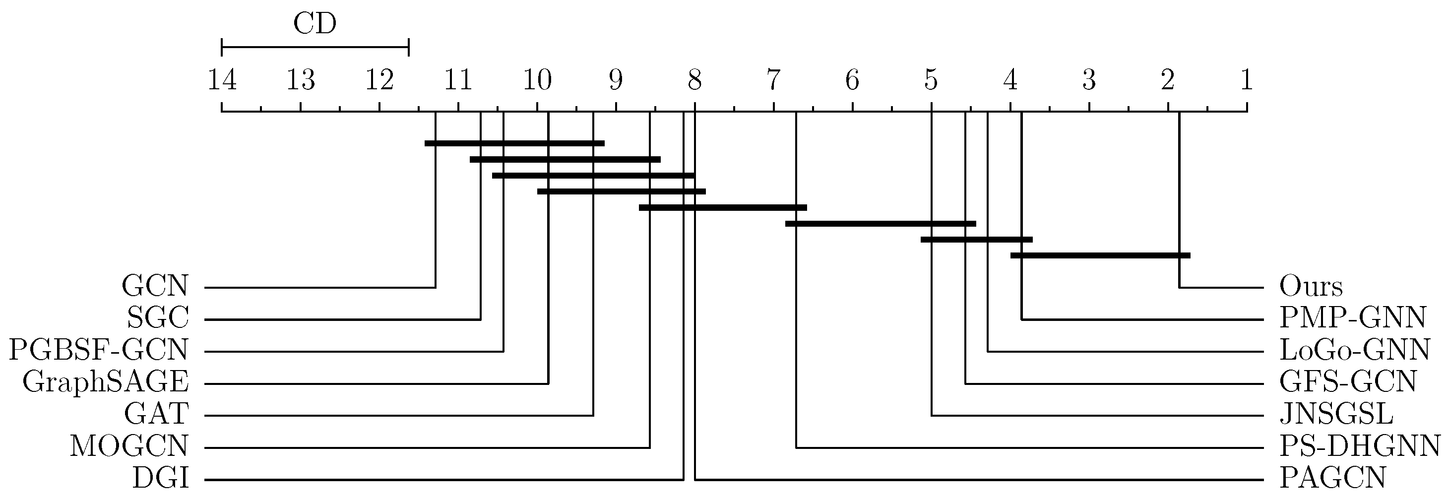
To further examine whether the observed performance differences are statistically reliable, we conduct a Friedman test followed by a Bonferroni–Dunn post hoc test on all datasets [47]. The Friedman test confirms that the compared methods do not perform equivalently, and the Bonferroni–Dunn test is then used to analyze the pairwise differences between our method and the baselines.

Figure 5 shows the Bonferroni–Dunn test results. The horizontal axis represents the average rank of each method, where a lower rank indicates better overall performance. The critical difference (CD) at $\alpha =0.05$ is 2.3714. Our method achieves the best average rank among all compared methods. Moreover, the rank differences between ours and most baselines exceed one CD, indicating statistically significant improvements over the majority of competing methods. These results provide additional evidence for the overall competitiveness of the proposed method.

4.4. Ablation Study

To demonstrate the significance of the proposed components, we design four representative variants and evaluate them on the benchmark datasets. Specifically, GFS denotes the original feature-splitting backbone adopted from GFS-GCN. Based on this backbone, we construct several variants to examine the contributions of CSA and DPTR. OURS-w-GFS denotes the basic GFS backbone without CSA or DPTR. OURS-w/o-DI removes dual-branch interaction and applies only single-channel polarized topology refinement after GFS. OURS-w/o-DPTR keeps CSA but removes DPTR, and thus focuses on improving the reliability of feature-wise propagation preference estimation. OURS-w/o-CSA keeps DPTR but removes CSA, and thus focuses on refining the propagation topology after feature splitting. The complete model is denoted as OURS. From Table 6, the following observations can be made:

(1)

The complete model achieves the best results on all seven datasets, suggesting that CSA and DPTR provide complementary benefits around the GFS backbone.

(2)

The inferior performance of OURS-w/o-DI suggests that single-channel polarization after feature splitting is insufficient. In contrast, the stronger results of OURS-w/o-CSA indicate that dual-branch coordination plays an important role in topology refinement.

(3)

Compared with OURS-w-GFS, the improvements of OURS-w/o-DPTR on citation datasets suggest that CSA helps stabilize feature-preference estimation. Likewise, the gains of OURS-w/o-CSA over OURS-w-GFS on several datasets indicate that topology refinement after feature splitting is beneficial for alleviating feature–topology mismatch.

Table 6. ACC (%) of CSA-PTR and its variants. Bold: best.

Methods	Cora	Citeseer	Pubmed	Actor	Texas	Cornell	Wisconsin	Average
OURS-w-GFS	81.7	71.6	81.8	33.5	72.9	64.8	70.5	68.1
OURS-w/o-DI	83.0	71.9	81.3	32.1	51.3	56.7	58.8	62.2
OURS-w/o-DPTR	83.8	71.8	82.5	33.4	70.2	51.3	68.6	65.9
OURS-w/o-CSA	84.4	72.5	82.7	33.0	67.5	70.2	64.7	67.9
OURS	84.7	72.9	82.9	35.4	75.6	72.9	76.4	71.6

Table 6. ACC (%) of CSA-PTR and its variants. Bold: best.

Methods	Cora	Citeseer	Pubmed	Actor	Texas	Cornell	Wisconsin	Average
OURS-w-GFS	81.7	71.6	81.8	33.5	72.9	64.8	70.5	68.1
OURS-w/o-DI	83.0	71.9	81.3	32.1	51.3	56.7	58.8	62.2
OURS-w/o-DPTR	83.8	71.8	82.5	33.4	70.2	51.3	68.6	65.9
OURS-w/o-CSA	84.4	72.5	82.7	33.0	67.5	70.2	64.7	67.9
OURS	84.7	72.9	82.9	35.4	75.6	72.9	76.4	71.6

The above ablation study verifies the module-level contribution of CSA and DPTR. In particular, removing either CSA or DPTR leads to performance degradation, indicating that reliable feature-preference estimation and topology refinement are both important for CSA-PTR. Since DPTR further introduces an auxiliary topology-coordination loss to guide the refined topology, we conduct an additional ablation study to isolate the contribution of each loss sub-term. Considering that this experiment focuses on verifying the loss mechanism rather than providing another full benchmark comparison, we report the results on three representative citation datasets. Specifically, OURS-w/o-${Loss}_{Lp}$ removes the entire auxiliary topology-coordination loss and uses only the task loss. OURS-w/o-${Loss}_{Post}$ removes the posterior pairwise consistency term and only keeps the graph Laplacian regularization term, while OURS-w/o-${Loss}_{Lap}$ removes the graph Laplacian regularization term and only keeps the posterior pairwise consistency term.

As shown in

Table 7. ACC (%) of CSA-PTR under different auxiliary loss variants. Bold: best.

Methods	Cora	Citeseer	Pubmed	Average
OURS-w/o-${Loss}_{Lp}$	82.2	72.0	82.2	78.8
OURS-w/o-${Loss}_{Post}$	84.3	72.8	82.7	79.9
OURS-w/o-${Loss}_{Lap}$	84.6	72.6	82.5	79.9
OURS	84.7	72.9	82.9	80.2

, removing the entire auxiliary topology-coordination loss leads to the largest performance degradation, with an average accuracy drop of 1.4 percentage points. This indicates that ${Loss}_{Lp}$ provides useful supervision for topology refinement beyond the task loss alone. When either the Laplacian regularization term or the posterior pairwise consistency term is removed, the performance remains better than the task-only variant but lower than the full model. This demonstrates that the graph Laplacian term and the posterior pairwise term provide complementary structural and semantic constraints, and their joint use leads to the best overall performance.

4.5. Parameter Sensitivity

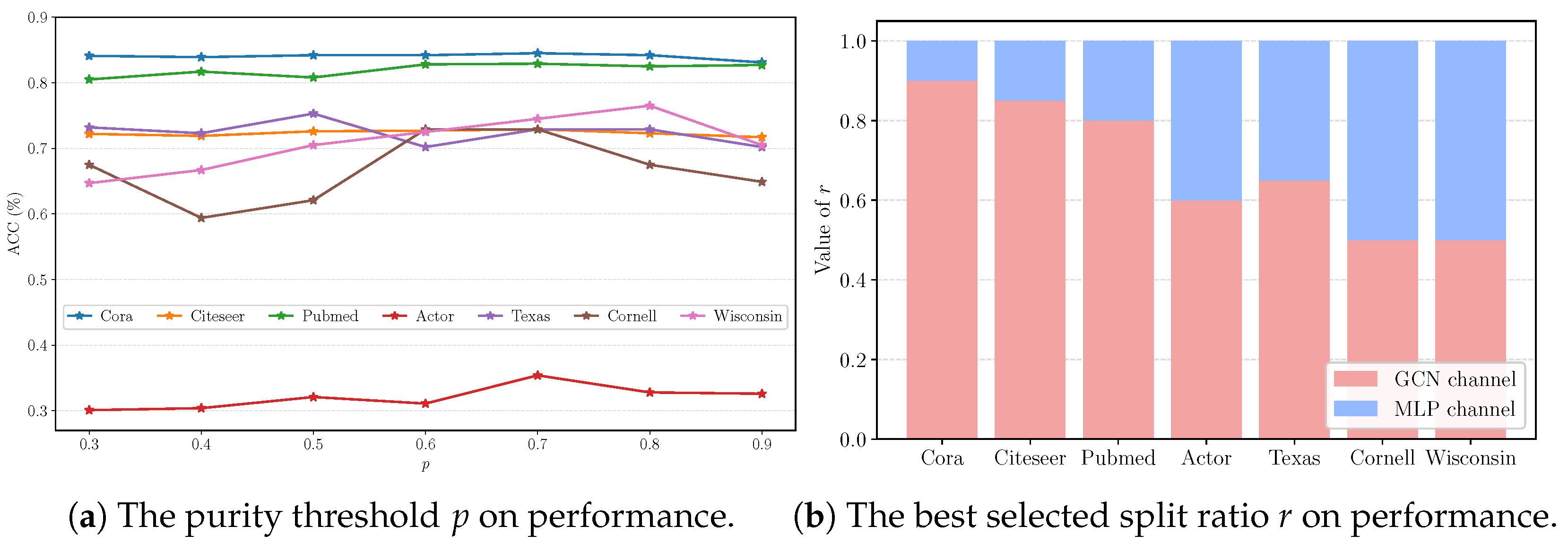
In this subsection, we analyze the sensitivity of CSA-PTR to two key hyper parameters, namely the split ratio r and the purity threshold p. The corresponding results are shown in Figure 6.

The purity threshold p controls how strictly local purity is enforced in CSA. A larger p imposes a stronger purity constraint within each granular ball, whereas a smaller p allows nodes with more diverse characteristics to be grouped together. To study its effect, we vary p from 0.3 to 0.9 and report the corresponding node classification accuracy on seven benchmark datasets, as shown in Figure 6a. Overall, the performance remains relatively stable when p ranges from 0.6 to 0.8, suggesting that a moderate purity constraint is generally more suitable. This observation indicates that overly small p may retain excessive local mixing, while overly large p may lead to excessively fragmented partitions and weaken stable contextual support. We also observe dataset-specific preferences. For example, Wisconsin performs poorly when p is small, whereas Cornell becomes worse when p is too large. Therefore, a moderate purity threshold usually provides a better balance between local coherence and structural stability.

The split ratio r determines how many feature dimensions are assigned to the graph-aware branch and the graph-agnostic branch in GFS. We use Bayesian optimization to select the optimal value of r for each dataset, and the resulting values are illustrated in Figure 6b. We observe that the citation datasets tend to prefer a larger graph-aware proportion, indicating that more feature dimensions can benefit from topology-guided propagation in these datasets. By contrast, the other datasets favor a more balanced split between the two branches. This observation is consistent with the motivation of feature splitting: the benefit of graph propagation is feature-dependent and dataset-dependent rather than uniform across the full feature space. Overall, the observed distribution of r further supports the necessity of selectively assigning different feature dimensions to different processing branches.

The effects of r and p reflect a dataset-specific tradeoff. A larger r sends more features to the graph branch and can exploit useful topology, but may also propagate graph-disfavored dimensions when topology-feature alignment is weak. Similarly, a low p may retain mixed boundary regions, whereas an overly high p may over-split local contexts. Therefore, moderate values usually provide a better balance between structural utilization, boundary suppression, and contextual preservation.

4.6. Visualization

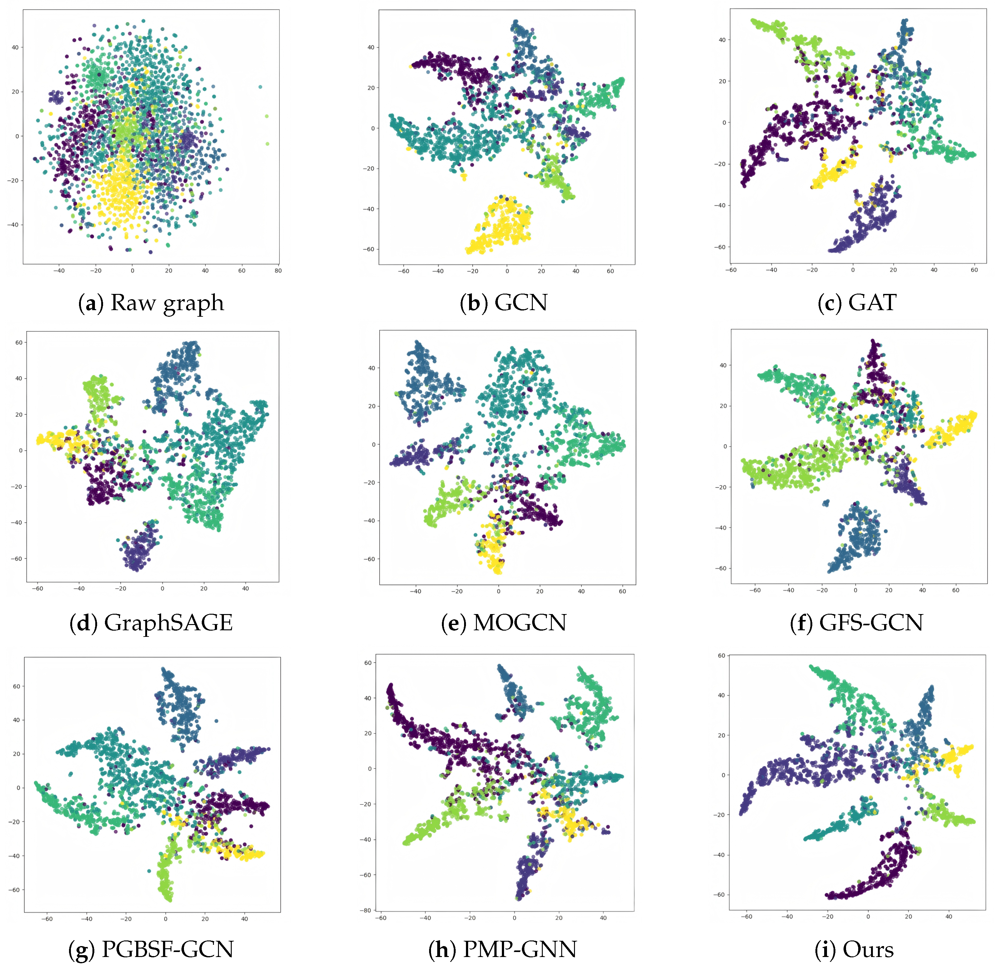
To further demonstrate the differences between CSA-PTR and the compared methods, we visualize the learned node representations via t-SNE by reducing them to a two-dimensional space [48]. The visualization results on the Cora dataset are shown in Figure 7.

As shown in Figure 7, the raw graph exhibits a highly chaotic distribution, where samples from different classes are heavily mixed and no clear class-wise structure can be observed. After graph learning, the compared methods can separate several classes to different degrees, but obvious overlaps still remain in many cases. In particular, although methods such as GCN, GAT and GraphSAGE can already form several visible clusters, the distributions are still relatively scattered and some classes remain mixed in the central region. GFS-GCN, PGBSF-GCN, and PMP-GCN further improve the class-wise structure, but there are still noticeable overlaps among different classes. By contrast, the embeddings learned by our model exhibit clearer class boundaries and more compact intra-class distributions. This visualization provides an intuitive illustration that the embeddings learned by CSA-PTR exhibit clearer inter-class separation and more compact intra-class distributions, which is broadly consistent with the quantitative results.

4.7. Framework Study

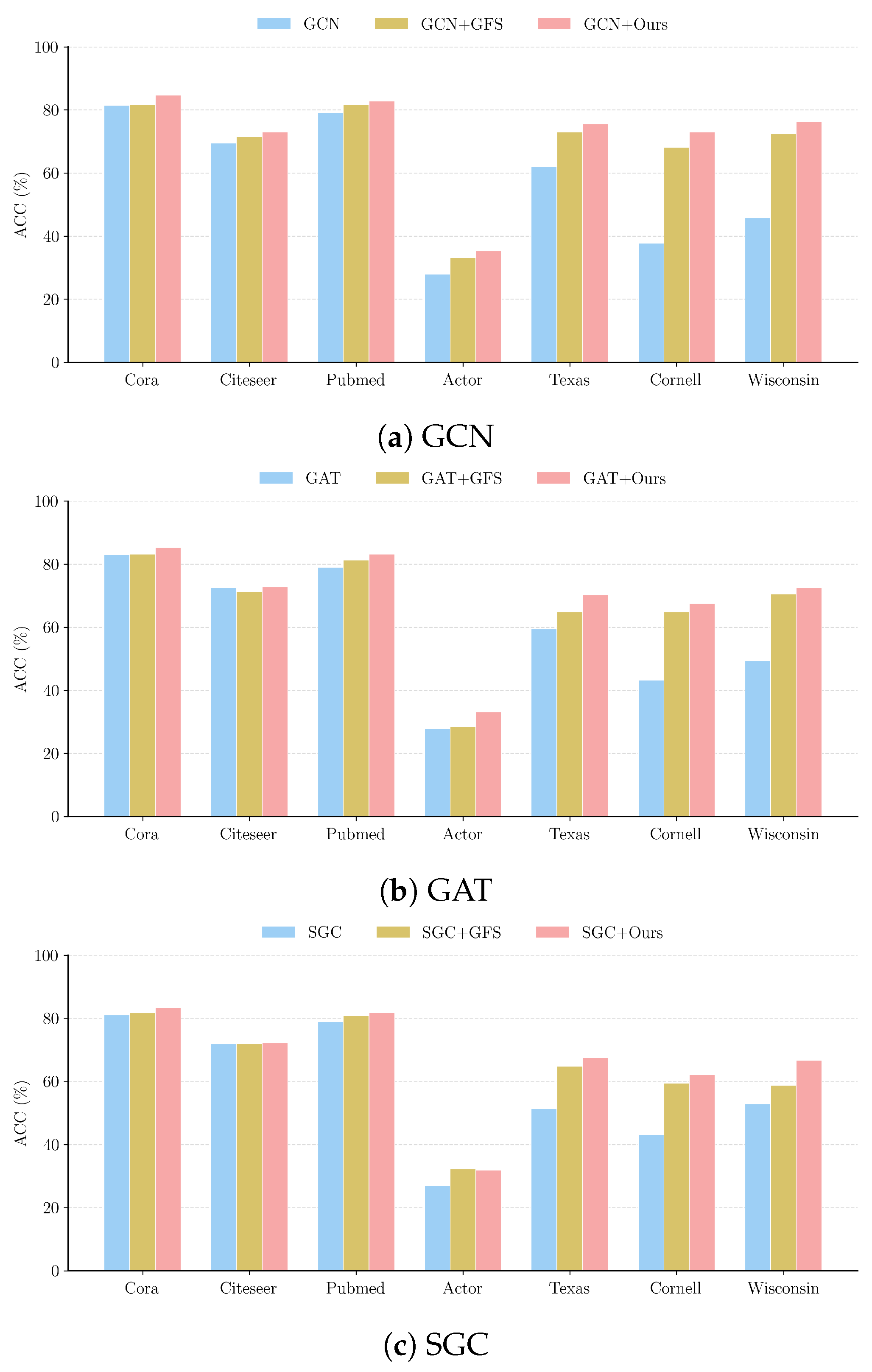
As previously described, CSA-PTR can be integrated into different GNN encoders in a relatively modular manner. To evaluate its generality, we instantiate it on three representative backbones and compare the resulting models with the corresponding original backbones as well as their GFS-based variants, where GFS refers to the basic feature-splitting module that partitions features according to their propagation preference for GNNs. The corresponding results are shown in Figure 8, from which two observations can be made.

First, CSA-PTR consistently improves the three representative backbones on most datasets, suggesting that the proposed framework is not restricted to a specific encoder and exhibits encouraging generality across the evaluated backbones.

Second, although the GFS-based variants already improve the original backbones in many cases, the full CSA-PTR framework still achieves better results in most settings. This suggests that basic feature splitting is beneficial, but that further improvement can be obtained by jointly enhancing preference estimation and post-splitting topology refinement.

5. Conclusions

In this paper, we revisit feature splitting in GNNs through the lens of selective propagation. While feature splitting offers a principled way to decide which dimensions to propagate, our analysis reveals two practical pitfalls on real-world graphs: unreliable propagation-preference estimation in locally mixed regions, and feature–topology mismatch after splitting. To address these issues, we propose CSA-PTR, a plug-and-play framework that enhances both estimation and propagation. Specifically, CSA constructs a purity-aware core–shell context for more reliable preference estimation, while DPTR refines the topology used by the graph-favored branch via polarized relation modeling and dual-branch posterior coordination.

Extensive experiments on seven benchmarks show that CSA-PTR achieves competitive or superior performance against strong baselines. Ablations confirm that CSA and DPTR offer complementary gains—CSA improves estimation reliability, and DPTR alleviates feature–topology mismatch. Additional results under varying label rates, statistical tests, sensitivity analysis, visualizations, and framework studies further attest to its effectiveness and robustness. Although the evaluated datasets cover multiple graph domains and supervision settings, the current experiments are mainly conducted on small-to-medium-scale benchmark graphs. Therefore, this study focuses on validating the effectiveness of CSA-PTR for reliable feature splitting and topology refinement under standard semi-supervised node classification settings. In addition, the full-batch pairwise topology-refinement design in DPTR makes experiments on very large graphs computationally demanding under the available hardware resources. Future work will explore scalable variants of CSA-PTR, such as mini-batch training, neighbor sampling, and anchor-based approximation, to extend the framework to larger graph scenarios.

References

1. Zhou, J.; Cui, G.; Hu, S.; Zhang, Z.; Yang, C.; Liu, Z.; Wang, L.; Li, C.; Sun, M. Graph neural networks: A review of methods and applications. AI Open 2020, 1, 57–81. [Google Scholar] [CrossRef]
2. Zhang, P.; Yan, Y.; Zhang, X.; Li, C.; Wang, S.; Huang, F.; Kim, S. TransGNN: Harnessing the Collaborative Power of Transformers and Graph Neural Networks for Recommender Systems. In Proceedings of the 47th International ACM SIGIR Conference on Research and Development in Information Retrieval, Washington, DC, USA, 14–18 July 2024. [Google Scholar]
3. Xia, L.; Huang, C.; Xu, Y.; Dai, P.; Bo, L. Multi-Behavior Graph Neural Networks for Recommender System. IEEE Trans. Neural Netw. Learn. Syst. 2024, 35, 5473–5487. [Google Scholar] [PubMed]
4. Rollins, Z.A.; Cheng, A.C.; Metwally, E. MolPROP: Molecular Property prediction with multimodal language and graph fusion. J. Cheminformatics 2024, 16, 56. [Google Scholar] [CrossRef]
5. Gao, Q.; Balhorn, L.S.; Laera, A.; Meys, R.; Goßen, J.; Weber, J.M.; Wernet, G.; Schweidtmann, A.M. Environmental impacts prediction using graph neural networks on molecular graphs. Comput. Chem. Eng. 2026, 204, 109362. [Google Scholar]
6. Ju, W.; Zhao, Y.; Qin, Y.; Yi, S.; Yuan, J.; Xiao, Z.; Luo, X.; Yan, X.; Zhang, M. COOL: A Conjoint Perspective on Spatio-Temporal Graph Neural Network for Traffic Forecasting. Inf. Fusion 2024, 107, 102341. [Google Scholar] [CrossRef]
7. Fan, G.; Sabri, A.Q.M.; Rahman, S.S.A.; Pan, L. DynaKey-GNN: An efficient dynamic key-node multi-graph neural network for spatio-temporal traffic flow forecasting. Eng. Appl. Artif. Intell. 2025, 159, 111757. [Google Scholar]
8. Jiang, W.; Luo, J.; He, M.; Gu, W. Graph Neural Network for Traffic Forecasting: The Research Progress. ISPRS Int. J. Geo-Inf. 2023, 12, 100. [Google Scholar] [CrossRef]
9. Wu, Y.; Hu, X.; Fan, X.; Ma, W.; Gao, Q. Learning Data-Driven Propagation Mechanism for Graph Neural Network. Electronics 2023, 12, 46. [Google Scholar]
10. Li, Q.; Han, Z.; Wu, X. Deeper Insights Into Graph Convolutional Networks for Semi-Supervised Learning. In Proceedings of the Thirty-Second AAAI Conference on Artificial Intelligence, New Orleans, LA, USA, 2–7 February 2018. [Google Scholar]
11. Shi, M.; Tang, Y.; Zhu, X. Topology and Content Co-Alignment Graph Convolutional Learning. IEEE Trans. Neural Netw. Learn. Syst. 2022, 33, 7899–7907. [Google Scholar] [PubMed]
12. Luan, S.; Hua, C.; Xu, M.; Lu, Q.; Zhu, J.; Chang, X.W.; Fu, J.; Leskovec, J.; Precup, D. When Do Graph Neural Networks Help with Node Classification? Investigating the Homophily Principle on Node Distinguishability. In Proceedings of the 37th Annual Conference on Neural Information Processing Systems, Orleans, LA, USA, 10–16 December 2023. [Google Scholar]
13. Zhang, L.; Sun, H. ESA-GCN: An Enhanced Graph-Based Node Classification Method for Class Imbalance Using ENN-SMOTE Sampling and an Attention Mechanism. Appl. Sci. 2024, 14, 111. [Google Scholar]
14. Lee, S.Y.; Kim, S.; Bu, F.; Yoo, J.; Tang, J.; Shin, K. Feature Distribution on Graph Topology Mediates the Effect of Graph Convolution: Homophily Perspective. In Proceedings of the 41st International Conference on Machine Learning, Vienna, Austria, 21–17 July 2024. [Google Scholar]
15. Zheng, Y.; Li, X.; Luan, S.; Peng, X.; Chen, L. Let Your Features Tell The Differences: Understanding Graph Convolution By Feature Splitting. In Proceedings of the International Conference on Learning Representations, Singapore, 24–28 April 2025. [Google Scholar]
16. Jin, D.; Yu, Z.; Huo, C.; Wang, R.; Wang, X.; He, D.; Han, J. Universal Graph Convolutional Networks. In Proceedings of the 35th Annual Conference on Neural Information Processing Systems, Virtual, 6–14 December 2021. [Google Scholar]
17. Koeneman, S.H.; Cavanaugh, J.E. An Improved Asymptotic Test for the Jaccard Similarity Index for Binary Data. Stat. Probab. Lett. 2022, 184, 109375. [Google Scholar] [CrossRef]
18. Rossi, E.; Kenlay, H.; Gorinova, M.I.; Chamberlain, B.P.; Dong, X.; Bronstein, M.M. On the Unreasonable Effectiveness of Feature Propagation in Learning on Graphs with Missing Node Features. In Proceedings of the First Learning on Graphs Conference, Virtual, 9–12 December 2022. [Google Scholar]
19. Kipf, T.N.; Welling, M. Semi-Supervised Classification with Graph Convolutional Networks. In Proceedings of the 5th International Conference on Learning Representations, Toulon, France, 24–26 April 2017. [Google Scholar]
20. Velickovic, P.; Cucurull, G.; Casanova, A.; Romero, A.; Lio, P.; Bengio, Y. Graph Attention Networks. In Proceedings of the 6th International Conference on Learning Representations, Vancouver, BC, Canada, 30 April–3 May 2018. [Google Scholar]
21. Zeng, H.; Zhou, H.; Srivastava, A.; Kannan, R.; Prasanna, V. GraphSAINT: Graph Sampling Based Inductive Learning Method. In Proceedings of the 8th International Conference on Learning Representations, Virtual, 26 April–1 May 2020. [Google Scholar]
22. Abu-El-Haija, S.; Perozzi, B.; Kapoor, A.; Alipourfard, N.; Lerman, K.; Harutyunyan, H.; Ver Steeg, G.; Galstyan, A. MixHop: Higher-Order Graph Convolutional Architectures via Sparsified Neighborhood Mixing. In Proceedings of the 36th International Conference on Machine Learning, Long Beach, CA, USA, 9–15 June 2019. [Google Scholar]
23. Luo, Z.; Lian, J.; Huang, H.; Jin, H.; Xie, X. Ada-GNN: Adapting to Local Patterns for Improving Graph Neural Networks. In Proceedings of the 15th ACM International Conference on Web Search and Data Mining, Tempe, AZ, USA, 21–25 February 2022. [Google Scholar]
24. Wang, Z.; Wei, Z.; Li, Y.; Kuang, W.; Ding, B. Graph Neural Networks with Node-wise Architecture. In Proceedings of the 28th ACM SIGKDD Conference on Knowledge Discovery and Data Mining, Washington, DC, USA, 14–18 August 2022. [Google Scholar]
25. Chien, E.; Peng, J.; Li, P.; Milenkovic, O. Adaptive Universal Generalized PageRank Graph Neural Network. In Proceedings of the 9th International Conference on Learning Representations, Virtual, 3–7 May 2021. [Google Scholar]
26. Luan, S.; Hua, C.; Lu, Q.; Zhu, J.; Zhao, M.; Zhang, S.; Chang, X.W.; Precup, D. Revisiting Heterophily For Graph Neural Networks. In Proceedings of the 36th Annual Conference on Neural Information Processing Systems, New Orleans, LA, USA, 28 November–9 December 2022. [Google Scholar]
27. Zhu, J.; Rossi, R.A.; Rao, A.; Mai, T.; Lipka, N.; Ahmed, N.K.; Koutra, D. Graph Neural Networks with Heterophily. In Proceedings of the 35th AAAI Conference on Artificial Intelligence, Virtual, 2–9 February 2021. [Google Scholar]
28. He, T.; Liu, Y.; Ong, Y.; Wu, X.; Luo, X. Polarized message-passing in graph neural networks. Artif. Intell. 2024, 331, 104129. [Google Scholar] [CrossRef]
29. Cong, H.; Yang, X.; Liu, K.; Guo, Q. Feature-topology cascade perturbation for graph neural network. Eng. Appl. Artif. Intell. 2025, 152, 110657. [Google Scholar] [CrossRef]
30. Teng, Q.; Liu, K.; Yang, X.; Li, M. Inconsistency-Aware Graph Convolutional Networks for Multi-View Classification. IEEE Trans. Emerg. Top. Comput. 2026, 10, 747–760. [Google Scholar]
31. Belghazi, M.I.; Baratin, A.; Rajeswar, S.; Ozair, S.; Bengio, Y.; Courville, A.; Hjelm, D. Mutual Information Neural Estimation. In Proceedings of the 35th International Conference on Machine Learning, Stockholm, Sweden, 10–15 July 2018. [Google Scholar]
32. Zheng, Y.; Luan, S.; Chen, L. What Is Missing In Homophily? Disentangling Graph Homophily For Graph Neural Networks. In Proceedings of the 38th Annual Conference on Neural Information Processing Systems, Vancouver, BC, Canada, 10–15 December 2024. [Google Scholar]
33. Wang, W.; Yang, X.; Zhang, Q.; Xia, S.; Yang, J.; Xu, T. Capturing local and global information: Multi-view graph convolutional network via granular-ball computing and collaborative matrix. Expert Syst. Appl. 2026, 296, 129057. [Google Scholar]
34. Wang, Y.; Yang, X.; Sun, Q.; Qian, Y.; Guo, Q. Purity Skeleton Dynamic Hypergraph Neural Network. Neurocomputing 2024, 610, 128539. [Google Scholar] [CrossRef]
35. Ullah, A.; Wang, B.; Sheng, J.; Long, J.; Khan, N.; Sun, Z. Identifying vital nodes from local and global perspectives in complex networks. Expert Syst. Appl. 2021, 186, 115778. [Google Scholar] [CrossRef]
36. Jebara, T.; Kondor, R.; Howard, A. Probability Product Kernels. J. Mach. Learn. Res. 2004, 5, 819–844. [Google Scholar]
37. Baradaaji, A.; Dornaika, F. Joint Latent Space and Label Inference Estimation with Adaptive Fused Data and Label Graphs. ACM Trans. Intell. Syst. Technol. 2023, 14, 62. [Google Scholar] [CrossRef]
38. Pei, H.; Wei, B.; Chang, K.C.; Lei, Y.; Yang, B. Geom-GCN: Geometric Graph Convolutional Networks. In Proceedings of the 8th International Conference on Learning Representations, Addis Ababa, Ethiopia, 26–30 April 2020. [Google Scholar]
39. Hamilton, W.L.; Ying, Z.; Leskovec, J. Inductive Representation Learning on Large Graphs. In Proceedings of the 31st International Conference on Neural Information Processing Systems, Long Beach, CA, USA, 4–9 December 2017. [Google Scholar]
40. Wu, F.; Souza, A., Jr.; Zhang, T.; Fifty, C.; Yu, T.; Weinberger, K. Simplifying Graph Convolutional Networks. In Proceedings of the 36th International Conference on Machine Learning, Long Beach, CA, USA, 9–15 June 2019. [Google Scholar]
41. Velickovic, P.; Fedus, W.; Hamilton, W.L.; Liò, P.; Bengio, Y.; Hjelm, R.D. Deep Graph Infomax. In Proceedings of the 7th International Conference on Learning Representations, New Orleans, LA, USA, 6–9 May 2019. [Google Scholar]
42. Wang, J.; Liang, J.; Cui, J.; Liang, J. Semi-supervised learning with mixed-order graph convolutional networks. Inf. Sci. 2021, 573, 171–181. [Google Scholar]
43. Cong, H.; Sun, Q.; Yang, X.; Liu, K.; Qian, Y. Enhancing graph convolutional networks with progressive granular ball sampling fusion: A novel approach to efficient and accurate GCN training. Inf. Sci. 2024, 676, 120831. [Google Scholar] [CrossRef]
44. Guo, Q.; Yang, X.; Zhang, F.; Xu, T. Perturbation-augmented Graph Convolutional Networks: A Graph Contrastive Learning architecture for effective node classification tasks. Eng. Appl. Artif. Intell. 2024, 129, 107616. [Google Scholar]
45. Guo, Q.; Yang, X.; Li, M.; Qian, Y. Collaborative graph neural networks for augmented graphs: A local-to-global perspective. Pattern Recognit. 2025, 158, 111020. [Google Scholar]
46. Liu, H.; Wu, J.; Li, W.; Yu, X. Graph structure learning with joint node and structural feature representation for node classification. Neurocomputing 2026, 663, 132002. [Google Scholar]
47. Dunn, O.J. Multiple Comparisons Among Means. J. Am. Stat. Assoc. 1961, 56, 52–64. [Google Scholar] [CrossRef]
48. van der Maaten, L.; Hinton, G. Visualizing Data using t-SNE. J. Mach. Learn. Res. 2008, 9, 2579–2605. [Google Scholar]
Figure 1. Boundary-induced bias in estimating TFI for selective propagation. (a) Illustration of a class-pair subgraph. Solid ellipses delineate two class-specific intra-class core regions (blue: Class A; red: Class B), while the dashed ellipse highlights class-boundary nodes that lie between the two cores and connect to both sides, potentially yielding label-inconsistent neighborhoods. (b) TFI scores are computed using a mutual-information criterion over the Core, Global, and Boundary regions for the original and clustered features. Boundary nodes show markedly lower TFI scores, while the clustering-based method improves the boundary-region TFI and raises the overall estimate.
Electronics 15 02882 g001
Figure 2. Feature–topology mismatch of split features on the original topology. Compared with the original features, split features yield lower Edge Overlap and Jaccard but higher smoothness energy, indicating degraded feature–topology compatibility after feature splitting.
Electronics 15 02882 g002
Figure 4. The figure provides an illustrative comparison of clustering behaviors. In this figure, red dots represent class A, blue dots represent class B, and the overlapping region on the right indicates the boundary area. From left to right are the ground-truth labels, granular-ball clustering, and k-NN clustering. Compared with k-NN clustering, granular-ball clustering produces cleaner local partitions around boundary regions.
Electronics 15 02882 g004
Figure 5. Bonferroni–Dunn post hoc test results of all comparison methods. The horizontal axis denotes the average rank, where lower ranks indicate better overall performance. Bold lines indicate methods whose rank differences are within the CD threshold.
Electronics 15 02882 g005
Figure 6. Parameter sensitivity analysis of CSA-PTR.
Electronics 15 02882 g006
Figure 7. Visualized results. Different colored dots represent the actual category of each node.
Electronics 15 02882 g007
Figure 8. Framework study of CSA-PTR on three representative backbones.
Electronics 15 02882 g008