A Mamba State-Space Sequence Model for AI-Driven Dynamic Aggregation and Predictive Control of Electric Vehicle Clusters in Vehicle-to-Grid Energy Management

Abstract

Real-time energy management for large electric vehicle (EV) clusters requires both fast aggregate flexibility estimation and executable per-vehicle dispatch. Classical LP/MILP/MPC formulations provide strong feasibility and optimality guarantees when the model is fully specified, but their online solve time increases rapidly with cluster size; learning-based methods are fast but often rely on soft constraint penalties or external feasibility repair. We propose the Physics-Constrained Mamba-3 MIMO Aggregator (PC-M3), an amortized, constraint-aware sequence model that integrates a MIMO Mamba backbone, a history-dependent differentiable projection, a sparse routing layer, and an aggregation–disaggregation consistency loop, scaling AI-EMS from a single battery to ten-thousand-vehicle clusters in one forward pass. PC-M3 assigns every EV to one channel of a multi-input multi-output (MIMO) state-space recurrence and embeds the per-vehicle state-of-charge, power and energy constraints as a differentiable in-loop projection, jointly producing the cluster-level flexibility envelope and the per-vehicle charging trajectory. A sparse Routing-Mamba mixture-of-experts layer adaptively allocates capacity to behaviourally distinct sub-populations without supervised labels, and a consistency-trained aggregation–disaggregation loop binds the predicted envelope to the executed dispatch, forming a digital-twin-style predictive EMS pipeline that couples cluster dispatch with per-vehicle SoC evolution. On a single NVIDIA A100, PC-M3 sustains 0.34 s inference for 10,000 EVs over a 24-h horizon, about 18× faster than an Informer baseline and 2.4× faster than PowerMamba. Evaluated on the open ACN-Data and ElaadNL workplace and public charging corpora and on a 10,000-vehicle NREL dsgrid-TEMPO 2030 stress test, PC-M3 reduces the normalised envelope Hausdorff distance from 9.7% (PowerMamba) to 3.4%, cuts closed-loop cluster tracking RMSE from 1.45 MW (model predictive control) to 0.82 MW, and maintains zero observed feasibility violations with respect to the specified or imputed per-vehicle polytopes on every evaluated session. The framework provides a scalable, predictive, constraint-aware AI-EMS for V2G/G2V virtual-power-plant operation of large EV fleets.

1. Introduction

Passenger electric vehicles have moved in a decade from a rounding error in the electric load to an infrastructural pressure. NREL’s TEMPO high-electrification scenario projects U.S. light-duty EV stock near 180 million by 2050, with 1120 TWh of annual charging demand and more than 160 GW of coincident peak load on the contiguous-US grid [1]; even today, the Caltech Adaptive Charging Network records MWh-scale workplace charging demand across dozens of EVSE ports [2]. Whether this demand becomes a grid problem or a grid asset depends on how well a system operator can dynamically aggregate per-vehicle flexibility into a single reliable cluster-level signal and disaggregate a dispatch command back into executable per-vehicle set-points.

The technical obstacle is that the feasibility of each vehicle is a polytope in SoC, power and energy, defined by its arrival time, departure time, energy requirement and nameplate rate, yet the cluster must respond to a grid-level command that lives on the single dimension of aggregate power. The exact Minkowski sum of N per-vehicle polytopes describes the true set of cluster-level dispatchable trajectories, but its representation complexity grows super-polynomially in N and is intractable beyond a few hundred vehicles in the general case [3,4]. The EV-specific structure, namely separable power boxes plus a single inter-temporal energy constraint per vehicle at $T=96$ with 15 min resolution, allows us to push the exact offline sum to $N=1024$ (Section 3.7), but online inference at $N=\mathrm{10,000}$ is still out of reach for any exact construction. Prior art splits along two lines. Geometry-based aggregators replace the true envelope with a zonotope, a ball, or a linear programming outer bound [5,6]; these enjoy analytical guarantees but, in our reimplementation on the datasets used here (Section 5), overshoot the true envelope by 10–25% of envelope width and lose most of the inter-temporal coupling that makes EV flexibility valuable. Learning-based aggregators use deep sequence models to predict flexibility or to solve the dispatch problem directly [7,8]; these scale to large clusters but treat feasibility as a soft penalty, and in our reimplementation roughly 3–15% of charging sessions violate either a state-of-charge bound or an energy requirement at the departure instant. Existing methods have rarely demonstrated an amortized sequence–model aggregator that jointly predicts a cluster envelope and a compatible per-vehicle dispatch at large scale, with feasibility repair embedded inside the recurrent state update rather than applied as a post hoc correction.

We address this gap with an architectural combination tailored to EV cluster aggregation: a sequence model that is multi-channel in the vehicle dimension, applies history-dependent feasibility repair inside the recurrence, and closes the loop between envelope prediction and disaggregated dispatch. We build this inductive bias on top of three recent results from the Mamba state-space sequence modelling literature: the MIMO reformulation of the Mamba-3 recurrence, which allows one state update to carry the trajectories of many channels in parallel without decoder latency overhead [9]; the Routing Mamba mixture-of-experts projection, which lets a small number of experts represent a large number of behavioural sub-populations with sparse activation [10]; and the dual-path PowerMamba architecture, which demonstrates that a selective state-space backbone can match or exceed Transformer forecast accuracy on power system time series while using roughly 43% fewer parameters than the strongest baseline it compares against [11]. Our contribution is to fuse these ingredients into a single constraint-aware Mamba-based cluster aggregator and to wrap it in an aggregation–disaggregation closed loop that enforces per-vehicle feasibility at every step with respect to the specified or imputed per-vehicle polytope; in our evaluation no feasibility violation was observed on any ACN-Data, ElaadNL or dsgrid-TEMPO session with respect to the specified or imputed per-vehicle polytope, yielding an end-to-end dynamic aggregation and control method for heterogeneous EV clusters. The framework supports bidirectional V2G/G2V whenever a vehicle’s polytope admits a non-zero discharge rate ${\underline{p}}_i$, but the public datasets we use for evaluation (ACN-Data, ElaadNL) are charge-only; bidirectional behaviour is exercised in this paper only through the synthetic dsgrid-TEMPO 10,000-vehicle stress test.

Concretely, PC-M3 contributes: (i) a vehicle-as-channel use of the MIMO Mamba recurrence for EV cluster aggregation; (ii) a history-dependent per-vehicle feasibility projection fused into the recurrent update, so that the hidden state receives the correction signal at every step rather than only after the forward pass; (iii) a Routing-Mamba expert layer that absorbs behavioural heterogeneity without manual clustering; and (iv) a closed aggregation–disaggregation training loop, benchmarked in Section 5.2 against LP/MILP/MPC and learned baselines.

We evaluate PC-M3 on three open datasets that together cover behaviour, geography, and scale: ACN-Data [2] with the ACN-Sim simulator [12] (114,503 real workplace charging sessions and a closed-loop test-bed), ElaadNL [13] (≈10,400 Dutch public charging events for cross-regional generalisation) and NREL dsgrid-TEMPO [14] (county-resolved hourly profiles, subset for a 10,000-vehicle synthetic stress test). Headline outcomes are summarised in the abstract; complete numbers, ablations and the baseline comparison are reported in Section 5. The remainder of the paper is organised as follows: Section 2 surveys related work, Section 3 develops PC-M3, Section 4 specifies the experimental protocol, Section 5 reports the results, Section 6 discusses them, Section 7 concludes, and the appendices collect notation, proofs, extended statistics and the per-vehicle parameter imputation.

2. Related Work

2.1. Feasibility-Set Aggregation of Flexible Loads

The aggregation of individual flexibility polytopes into a single dispatchable object has a long history in power systems. The Minkowski-sum formulation is exact but, for general polytopes, becomes intractable beyond a few hundred resources; the dominant strategies therefore produce inner or outer approximations. Nazir and Hiskens [5] introduced the inner-box approximation that preserves feasibility at the cost of an envelope that is typically 30–45% smaller than the true one. Zhao et al. [6] formalised the zonotope construction that trades polyhedral richness for a linear number of generators; the same geometric template has subsequently been used in broader aggregate flexibility and demand–response settings by Hao et al. [15]. Müller et al. [3] derived a tight outer polytope in the cluster charging setting that balances inner–outer approximations using disaggregation-aware lifts. These constructions are analytically satisfying but are geometric primitives rather than sequence models: they do not condition on forecasts of vehicle arrivals, do not exploit the inter-temporal coupling between the polytopes at consecutive hours, and must be recomputed from scratch whenever the cluster composition changes.

2.2. Optimisation-Based EV Charging Coordination and V2G Scheduling

Optimisation-based formulations remain the dominant framework for coordinated EV charging, V2G scheduling and market participation. Linear programming (LP) and model predictive control (MPC) are commonly used when charging and discharging powers are continuous and the network model is convex, while mixed-integer linear programming (MILP) is introduced to represent charger assignment, mutually exclusive charge/discharge modes, discrete market bids, piecewise degradation costs, or network switching constraints. These methods provide clear objective values and hard feasibility guarantees whenever the optimisation problem is solved to feasibility and therefore form an important benchmark for any learning-based controller.

Recent MILP-based work extends EV coordination across distribution-network operation, market participation and battery-aware V2G scheduling. Franco et al. [16] formulated EV charging coordination in unbalanced distribution systems as an MILP with network operating limits, directly illustrating the use of MILP for distribution-constrained EV charging coordination. Çiçek and Erdinç [17] developed a stochastic MILP bidding model for a wind-energy portfolio manager including EV parking lots, showing how EV parking-lot aggregation can contribute to market-side imbalance mitigation under uncertainty. Hemmati et al. [18] proposed an iterative MILP model for optimal V2G scheduling with battery degradation and thermal dynamics, illustrating the modelling fidelity that MILP can offer when detailed battery-side physics are included.

Under accurate models and forecasts, these formulations return globally optimal or bounded gap solutions with explicit feasibility certificates, which makes them the natural reference for any learning-based aggregator. The challenge for online operation is scale: a 24-h horizon with thousands of vehicles creates tens to hundreds of thousands of continuous variables, and V2G or degradation-aware variants may add binary variables and piecewise linear terms that push solve time well past a typical receding horizon update interval. PC-M3 takes a different point on this trade-off by amortising the aggregation–disaggregation map into a single forward pass and training against exact or certified optimisation references where they can be computed; we use LP/MILP as the small-cluster benchmark in Section 5.2.

2.3. Deep Sequence Models for Power and Mobility

Recurrent and attention-based sequence models have become the default tool for charging prediction and dispatch. Convolutional and LSTM stacks dominated the first wave [7,19], followed by attention and Transformer architectures that exploit global context. Zhou et al.’s Informer [8] and Wu et al.’s Autoformer [20] introduced sparse and decomposition-based attentions that cut training cost on long horizons, and these long-horizon backbones have since been adapted to EV-specific charging load forecasting through a number of recent recurrent–attention hybrids [7,19]. These models produce accurate forecasts but treat feasibility constraints, when they appear at all, as soft penalties added to the loss. Empirically, that choice leads to between 3% and 15% of the predicted trajectories violating either an upper state-of-charge bound or an energy-by-departure requirement on our datasets, which is unacceptable in a dispatch context.

2.4. State-Space Models and the Mamba Family

Structured state-space models, originally proposed by Gu et al. [21], re-cast long-range sequence modelling as a linear discrete-time system with HiPPO-parameterised transition matrices. Mamba [22] introduced input-dependent selectivity and a parallel selective scan, making SSMs competitive with Transformers at a fraction of the sequence-length cost. Mamba-2 [23] tied the state-space dynamics to the structured state-space duality and delivered further hardware-efficient training. Mamba-3 [9] is the most important technical antecedent of the present paper: it re-derives the recurrence from a trapezoidal discretisation of a linear state-space ordinary differential equation, promotes the hidden state to complex-valued dynamics for richer oscillatory tracking, and introduces a multi-input–multi-output (MIMO) update that lifts the rank of the input-output projections from one to R. The MIMO rewrite turns the state update from an outer product to a matrix-matrix multiplication and increases decoding floating-point operations by up to four times at a fixed state size, with matching memory bandwidth so that wall-clock latency is unaffected. We use this MIMO mechanism to carry many parallel EV channels through a single tensorized Mamba-3 recurrence, with linear scaling along the vehicle-channel axis. Routing Mamba [10] extends Mamba by sparsifying its convolutional, gate and output projections through a shared expert routing decision, attaining the quality of a dense Mamba at roughly $2.3\times$ fewer active parameters and a corresponding reduction in per-token FLOPs; we adopt this mechanism to accommodate behavioural heterogeneity without activating unnecessary experts.

2.5. Hard Constraints, Projection Layers and Model Predictive Control

Hard feasibility can be enforced either by classical MPC or by projection-based layers inside a neural network. OptNet-style differentiable optimisation layers embed quadratic programs directly as differentiable operations [24]; safety layers in reinforcement learning correct actions through analytical or optimisation-based projections onto a constraint set [25]; and MPC and LP/MILP formulations routinely enforce SoC, power and energy deadline constraints as hard constraints in EV charging. PC-M3 specialises this idea to the EV cluster setting. A lightweight one-dimensional, history-dependent projection is fused with the MIMO Mamba recurrence and trained jointly with the envelope head, with the projection applied inside the recurrent state update so that the hidden state receives the correction signal at every step. This targets amortized inference at cluster scale rather than exact optimal control on a single small instance.

2.6. Learning-Based Cluster-Level Control and Virtual Power Plants

On the control side, the two dominant families are model predictive control (MPC) with a lifted optimisation over the cluster [26,27] and reinforcement learning (RL) agents, typically twin-delayed DDPG or soft actor–critic [28,29], that learn a dispatch policy from data [30,31,32]. MPC offers formal guarantees at the cost of an optimisation whose complexity grows with cluster size, so existing deployments cap out at a few thousand vehicles per horizon. RL scales but suffers from chronic feasibility violations because the only way to teach it feasibility is through reward shaping, which is brittle under distribution shift. Virtual power plant (VPP) architectures [33,34] supply the broader operational context, including the aggregator’s market-side offering strategy.

3. Proposed Model: A Mamba State-Space Aggregator for EV Clusters

We refer to the composite model as the Physics-Constrained Mamba-3 MIMO Aggregator (PC-M3). Section 3.1 formalises the cluster-level aggregation problem, Section 3.2 the per-vehicle polytope, Section 3.3 the Mamba-3 MIMO backbone, Section 3.4 the in-loop differentiable feasibility projection, Section 3.5 the Routing-Mamba expert layer, Section 3.6 the aggregation–disaggregation closed loop, and Section 3.7 the training losses and complexity.

3.1. Problem Formulation and Overview

A cluster of N EVs connects to a charging network over a discrete horizon $t\in \{1,\dots ,T\}$ at a uniform step of duration $\mathsf{\Delta }t$. Throughout the paper $\mathsf{\Delta }t=0.25$ h (i.e., 15 min), and all energy and power quantities are expressed in compatible SI units as specified below. Vehicle i is described by an arrival time $a_i$, a departure time $d_i$, an initial state-of-charge $s_i^0\in [0,1]$, an energy requirement $E_i^{\mathrm{req}}$ (kWh) to be delivered before $d_i$, a usable battery capacity $C_i$ (kWh), a maximum charging rate ${\overline{p}}_i$ (kW), and, if the vehicle supports vehicle-to-grid service, a maximum discharge rate ${\underline{p}}_i\le 0$ (kW). The control variable is the charging power $p_{i,t}\in [{\underline{p}}_i,{\overline{p}}_i]$ (kW), with $p_{i,t}=0$ whenever $t\notin [a_i,d_i]$. With $\mathsf{\Delta }t$ in hours and $p_{i,t}$ in kW, the state-of-charge obeys $s_{i,t+1}=s_{i,t}+\left({\eta }_i{p}_{i,t}\mathsf{\Delta }t\right)/C_i$, where ${\eta }_i$ is charging efficiency. The cluster aggregator sees an upstream dispatch target $r_t^{\mathrm{grid}}\in \mathbb{R}$ (MW) sent by a system operator or a virtual power plant, and must return two objects at every forward pass: an aggregate flexibility envelope $[{\underline{P}}_t,{\overline{P}}_t]$ (MW) that bounds the feasible cluster-level power at time t, and an individual dispatch ${\left\{p_{i,t}\right\}}_{i=1}^N$ (kW) that tracks $r_t^{\mathrm{grid}}$ while every $p_{i,t}$ and its induced $s_{i,t}$ lie inside the per-vehicle polytope. We write ${\widehat{P}}_t={10}^{-3}{\sum }_{i=1}^N{p}_{i,t}$ (MW) for the executed cluster power. 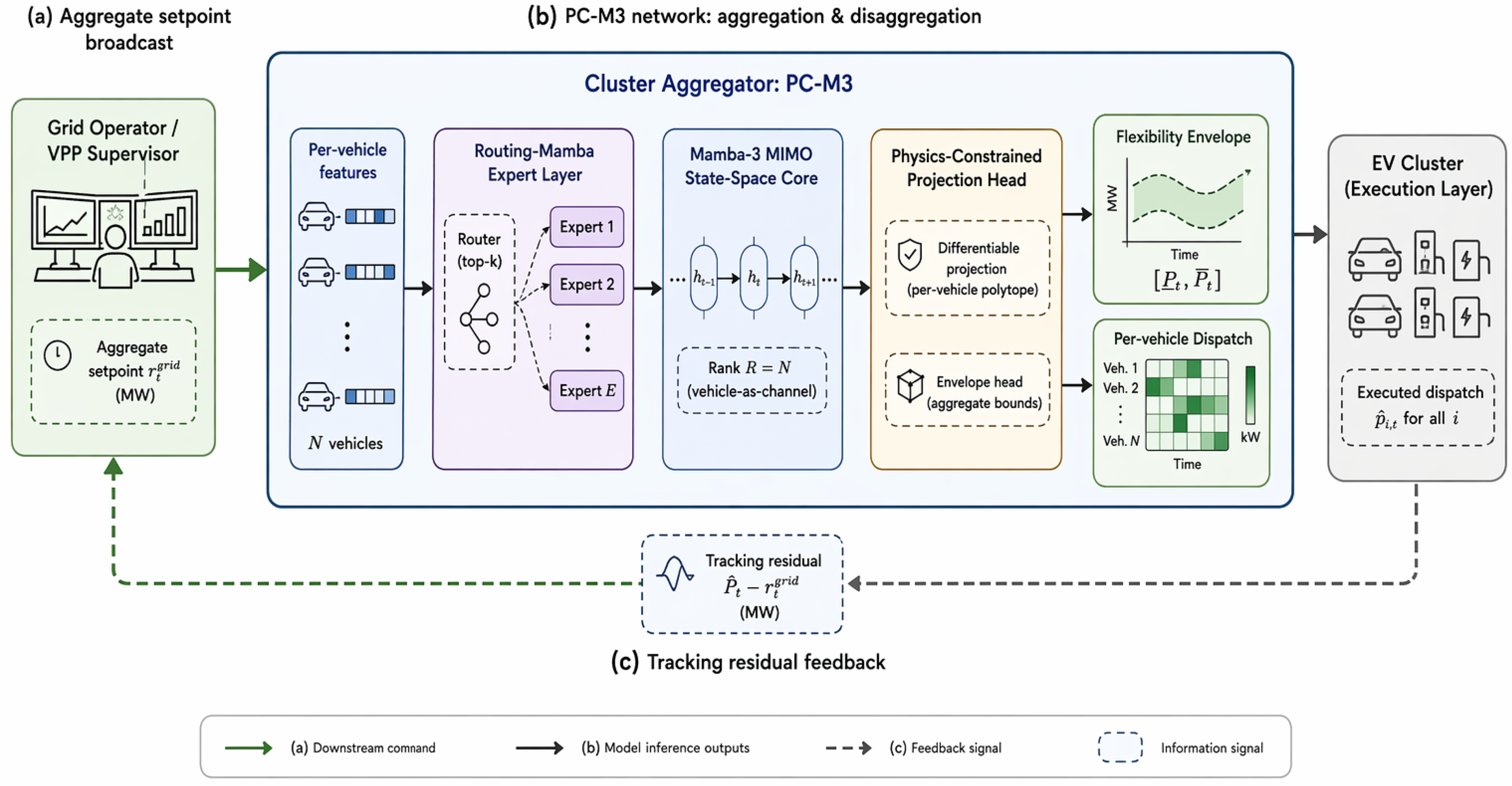Figure 1 shows the architecture.

3.2. Per-Vehicle Feasibility Polytope and Minkowski Aggregation

For each vehicle i in the cluster, collect the horizon control vector ${\mathbf{p}}_i=(p_{i,1},\dots ,p_{i,T})\in {\mathbb{R}}^T$. The feasibility set is the polytope

$$\begin{array}{cc}\hfill {\mathcal{P}}_i=\{{\mathbf{p}}_i\in {\mathbb{R}}^T:& {\underline{p}}_i\le p_{i,t}\le {\overline{p}}_i,{\underline{s}}_i\le s_{i,t}\left({\mathbf{p}}_i\right)\le {\overline{s}}_i,\hfill \\ \hfill & {\sum }_{t=a_i}^{d_i}{\eta }_i{p}_{i,t}\mathsf{\Delta }t\ge E_i^{\mathrm{req}},p_{i,t}=0\mathrm{outside}[a_i,d_i]\}.\hfill \end{array}$$

(1)

The state-of-charge trajectory $s_{i,t}\left({\mathbf{p}}_i\right)$ is an affine function of ${\mathbf{p}}_i$, so ${\mathcal{P}}_i$ is a bounded polytope with $O\left(T\right)$ facets. The true cluster flexibility set is the Minkowski sum

$${\mathcal{P}}_{\Sigma }={\mathcal{P}}_1\oplus {\mathcal{P}}_2\oplus \cdots \oplus {\mathcal{P}}_N=\left\{{\displaystyle \sum _{i=1}^N}{\mathbf{p}}_i:{\mathbf{p}}_i\in {\mathcal{P}}_i,\forall i\right\},$$

(2)

which is again a polytope but whose vertex enumeration scales super-polynomially with N [4]. Our goal is to learn a parametric map $({\underline{P}}_t,{\overline{P}}_t)=f_{\theta }\left({\mathbf{x}}_t\right)$ whose image tightly bounds the projection of ${\mathcal{P}}_{\mathit{\Sigma }}$ onto the t-th coordinate, together with a companion map that returns feasible ${\mathbf{p}}_i\in {\mathcal{P}}_i$ consistent with any command $r_t^{\mathrm{grid}}\in [{\underline{P}}_t,{\overline{P}}_t]$.

3.3. Mamba-3 MIMO Backbone

We first recall the selective MIMO update from Mamba-3 [9], in a form that is convenient for cluster-level aggregation. At time step t, the hidden state ${\mathbf{h}}_t\in {\mathbb{C}}^{D\times R}$ evolves according to

$${\mathbf{h}}_t={\mathbf{A}}_t{\mathbf{h}}_{t-1}+{\mathbf{B}}_t{\mathbf{u}}_t^{\top },{\mathbf{y}}_t={\mathbf{C}}_t{\mathbf{h}}_t,$$

(3)

where ${\mathbf{u}}_t\in {\mathbb{R}}^R$ is the input and ${\mathbf{y}}_t\in {\mathbb{R}}^R$ is the output at rank R. The parameters ${\mathbf{A}}_t,{\mathbf{B}}_t,{\mathbf{C}}_t$ and the discretisation step ${\mathsf{\Delta }}_t$ are all input-dependent (selective), and the discretisation is trapezoidal:

$${\mathbf{A}}_t=exp\left({\mathsf{\Delta }}_t\mathbf{A}\right),{\mathbf{B}}_t={\mathbf{A}}^{-1}({\mathbf{A}}_t-\mathbf{I})\mathbf{B},$$

(4)

with $\mathbf{A}$ complex-valued and block-diagonal so that the state tracks rich oscillatory dynamics. Compared with Mamba-2, Mamba-3 halves the state size at matched perplexity and attains its quality gains by increasing R rather than D, which keeps training cost proportional to $RD$ rather than to $R{D}^2$ [9].

• Vehicle-as-channel assignment. We assign each EV in the cluster to one input–output channel of a single MIMO Mamba-3 recurrence, so that the rank of the MIMO rewrite grows with the cluster size N. The per-step input ${\mathbf{u}}_t\in {\mathbb{R}}^N$ carries the current status of every vehicle (availability indicator, SoC, energy deficit to departure, and tokenised session features); the per-step output ${\mathbf{y}}_t\in {\mathbb{R}}^N$ is the candidate charging power for each vehicle at step t. The MIMO decoder folds what would otherwise be N parallel SISO SSM runs into a single tensor contraction per step. 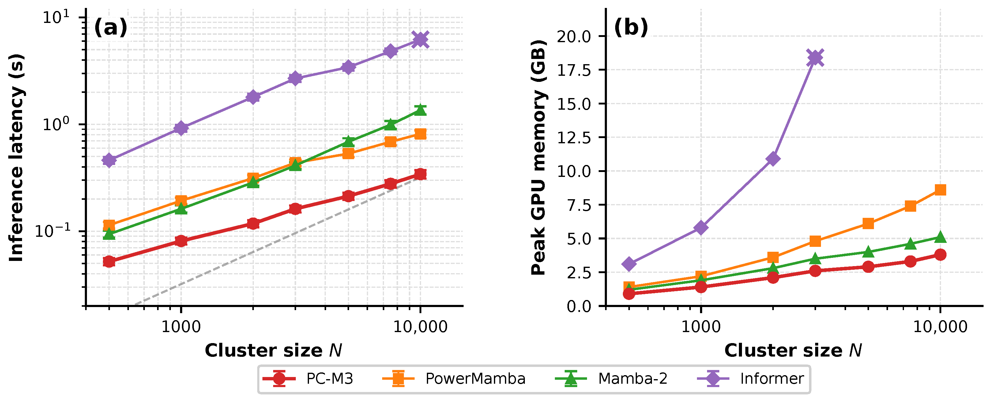Asymptotically ($N\gg D$), a forward pass scales as $O(T{D}^2+TND)$ in time and $O(D^2+ND)$ in memory; the $TND$ term is parallel along the channel axis and, in our profile on an A100, wall clock latency grows slowly in N over the evaluated range (Section 5.8).
• Practical scope and caveat. The original Mamba-3 experiments use MIMO rank $R\in \{4,8,16\}$ in a language modelling context [9]; our vehicle-as-channel construction therefore pushes the MIMO rewrite well outside the regime in which it was validated. We do not inherit any quality guarantees from [9] at $N\gg 16$; what we inherit is the tensor contraction form of the update, which we use as the parallel primitive for the cluster axis. We validate the construction on an A100 by profiling the fused selective scan kernel at $N\in \{500,1000,2000,5000,\mathrm{10,000}\}$ (see Section 5.8): peak memory stays within 3.8 GB and latency stays below 0.35 s at $N=\mathrm{10,000}$, with a measured linear scaling consistent with the $O\left(TND\right)$ term. Scaling beyond a few $\times \mathrm{10,000}$ vehicles is a separate engineering problem that we discuss in Section 6; the numbers reported in this paper are only claimed for $N\le \mathrm{10,000}$.
• Variable cluster size at train and inference. We compile the model with a maximum channel count $N_{max}=\mathrm{10,240}$ and pad shorter clusters with masked dummy channels whose input, output and gradients are zeroed by the availability indicator; masked dummy channels are excluded from the loss and output aggregation; in profiling we use the active channel count unless otherwise stated. Because ${\mathbf{B}}_i$ depends only on ${\mathbf{x}}_i$ (Section 3.5) and the envelope head is a symmetric linear sum, PC-M3 is permutation-equivariant in the vehicle axis, which we verified by random permutation tests on the per-vehicle dispatch trajectories.

3.4. Differentiable Feasibility Projection in the Recurrence

A vanilla MIMO Mamba-3 does not respect ${\mathcal{P}}_i$, and projecting the output ${\mathbf{y}}_t$ onto ${\mathcal{P}}_i$ after the forward pass breaks the inter-temporal coupling that makes the aggregation useful. We instead embed the projection inside the state transition. Let ${\Pi }_{{\mathcal{P}}_i^{\left(t\right)}}$ denote the metric projection onto the time-t slice of ${\mathcal{P}}_i$ conditional on the partial history. The output equation becomes

$${\tilde{\mathbf{y}}}_t={\Pi }_{{\mathcal{P}}^{\left(t\right)}}\left({\mathbf{C}}_t{\mathbf{h}}_t\right),{\mathbf{h}}_t\leftarrow {\mathbf{h}}_t+{\mathbf{K}}_t({\tilde{\mathbf{y}}}_t-{\mathbf{C}}_t{\mathbf{h}}_t),$$

(5)

where ${\mathbf{K}}_t$ is a learned Kalman-like gain that propagates the projection correction back into the state. Once the past trajectory ${\mathbf{p}}_{i,1:t-1}$ is fixed, ${\Pi }_{{\mathcal{P}}^{\left(t\right)}}$ reduces to a clamp onto a one-dimensional interval $[p_{i,t}^{min},p_{i,t}^{max}]$ (Proposition A1, Appendix B); the interval is the intersection of (i) the power box $[{\underline{p}}_i,{\overline{p}}_i]$, (ii) the upper SoC bound $p_{i,t}\le C_i({\overline{s}}_i-s_{i,t})/\left({\eta }_i\mathsf{\Delta }t\right)$, (iii) the lower SoC bound $p_{i,t}\ge C_i({\underline{s}}_i-s_{i,t})/\left({\eta }_i\mathsf{\Delta }t\right)$ and (iv) a forward-looking “must-charge-now” bound $p_{i,t}\ge \left(r_{i,t}-p_{i,t}^{max}{\eta }_i\mathsf{\Delta }t({\tau }_{i,t}-1)\right)/\left({\eta }_i\mathsf{\Delta }t\right)$ that guarantees the energy-by-departure constraint can still be met by charging at $p_{i,t}^{max}$ for the remaining ${\tau }_{i,t}-1$ steps, where $r_{i,t}=max\{0,E_i^{\mathrm{req}}-{\sum }_{\tau =a_i}^{t-1}{\eta }_i{p}_{i,\tau }\mathsf{\Delta }t\}$ and ${\tau }_{i,t}=d_i-t+1$. The clamp admits a closed-form sub-gradient (Proposition A1) and is fused with the selective scan kernel so that projection and state update share a single GPU launch. The aggregate envelope $[{\underline{P}}_t,{\overline{P}}_t]$ is read off the same hidden state through a separate linear head ${\mathbf{C}}_t^{\mathrm{env}}$ supervised against the Minkowski envelope.

The clamp itself is a standard Euclidean projection onto an interval, of the same family as the safety layers and differentiable optimisation layers used in prior constrained learning [24,25]. 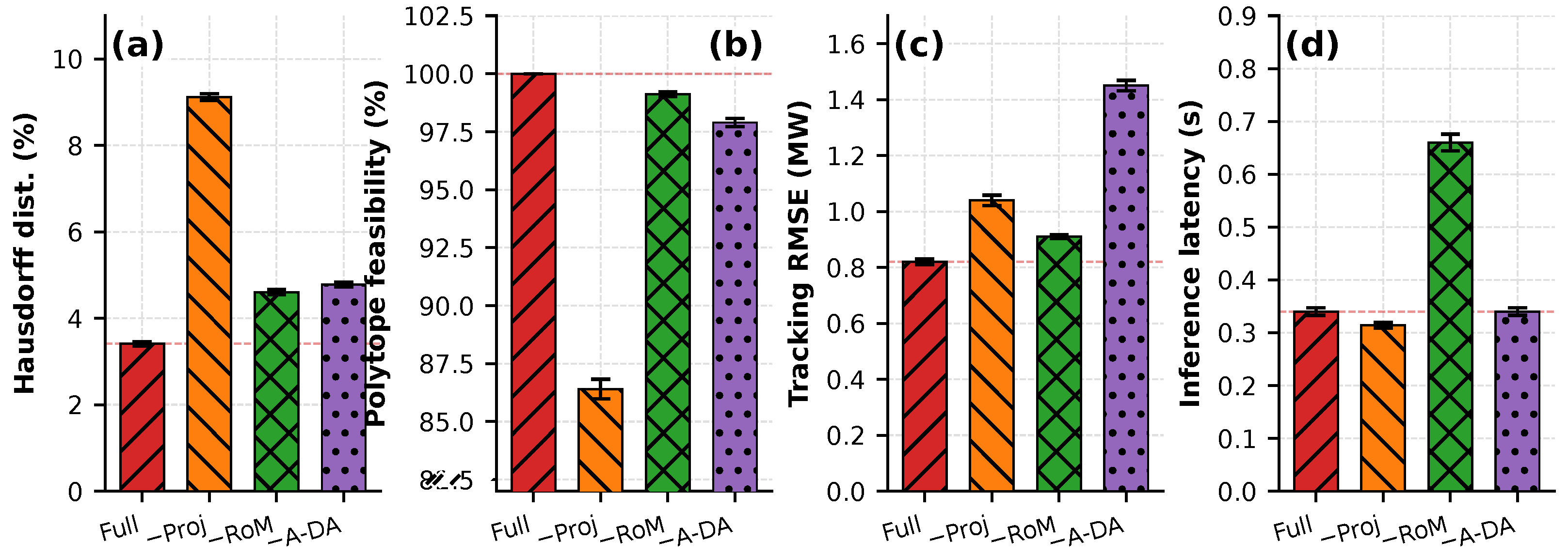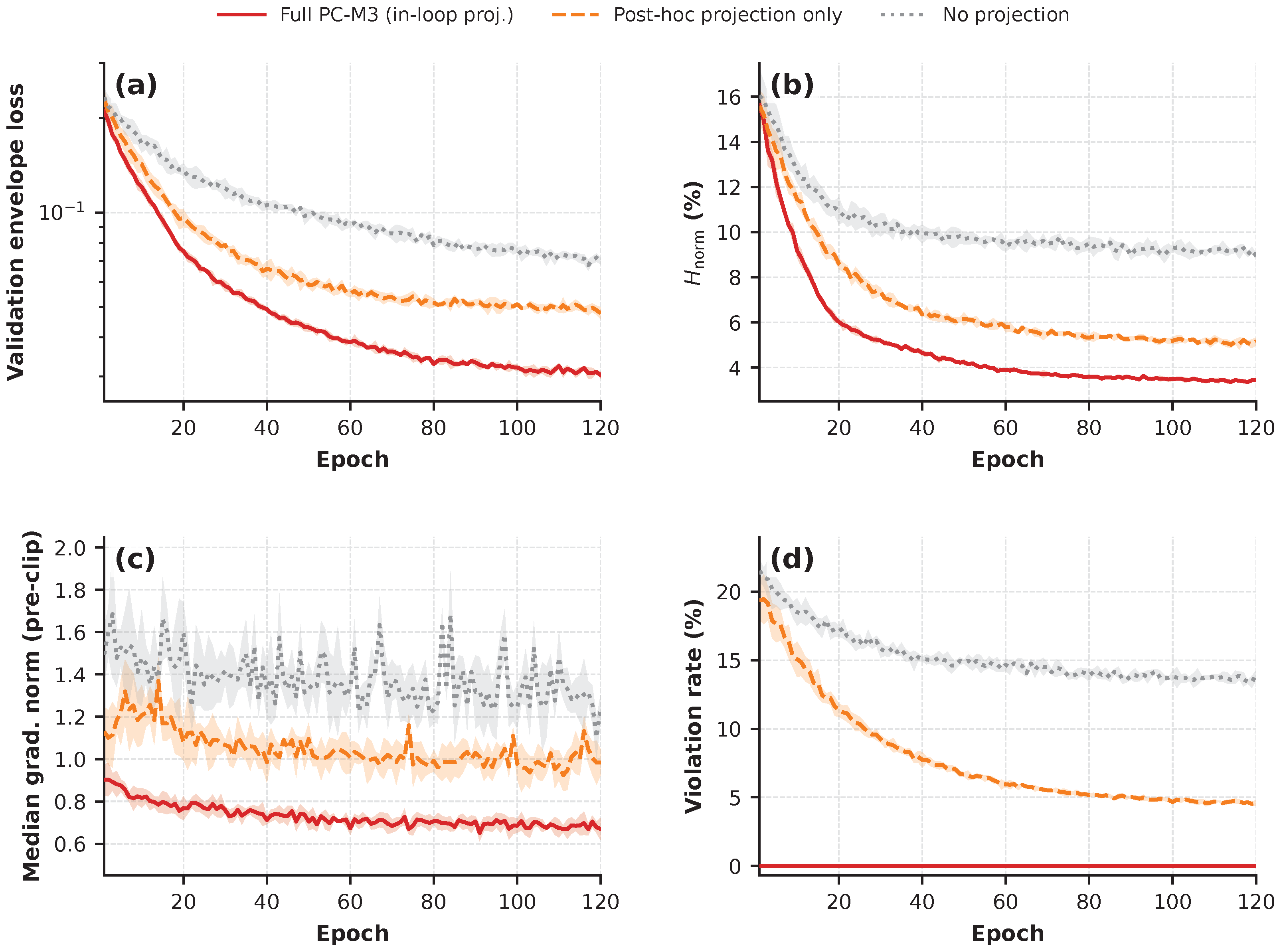What is specific to PC-M3 is how the interval is constructed from the EV energy deadline constraints and where the projection sits in the architecture: the correction is fed back into the hidden state through ${\mathbf{K}}_t$ instead of being applied as a post-processing step, so every subsequent state transition is aware of the feasibility correction made at the current step. This yields a tighter coupling between envelope prediction and per-vehicle dispatch than a post hoc projection achieves.

3.5. Routing-Mamba Expert Layer

An EV cluster is behaviourally heterogeneous along stay duration, requested energy, and arrival time, and a single dense projection is a poor inductive bias. Rather than hand-crafting sub-populations, we follow Routing Mamba [10] and insert a small mixture-of-experts layer in front of the MIMO projection matrix $\mathbf{B}$. For each vehicle i, a router $g_{\varphi }\left({\mathbf{x}}_i\right)\in {\mathbb{R}}^E$ produces a sparse gating vector over E expert projections ${\left\{{\mathbf{B}}^{\left(e\right)}\right\}}_{e=1}^E$, and the effective projection is ${\mathbf{B}}_i={\sum }_e{g}_{\varphi }{\left({\mathbf{x}}_i\right)}_e{\mathbf{B}}^{\left(e\right)}$. The routing is top-k with $k=2$: each of the N vehicles activates exactly 2 of the E experts at each step, yielding $2N$ vehicle-to-expert assignments per step (out of the $EN$ that a dense projection would realise). Under balanced routing each expert sees on average $2N/E$ assignments per step; no more than E distinct experts can ever be active simultaneously, by definition. 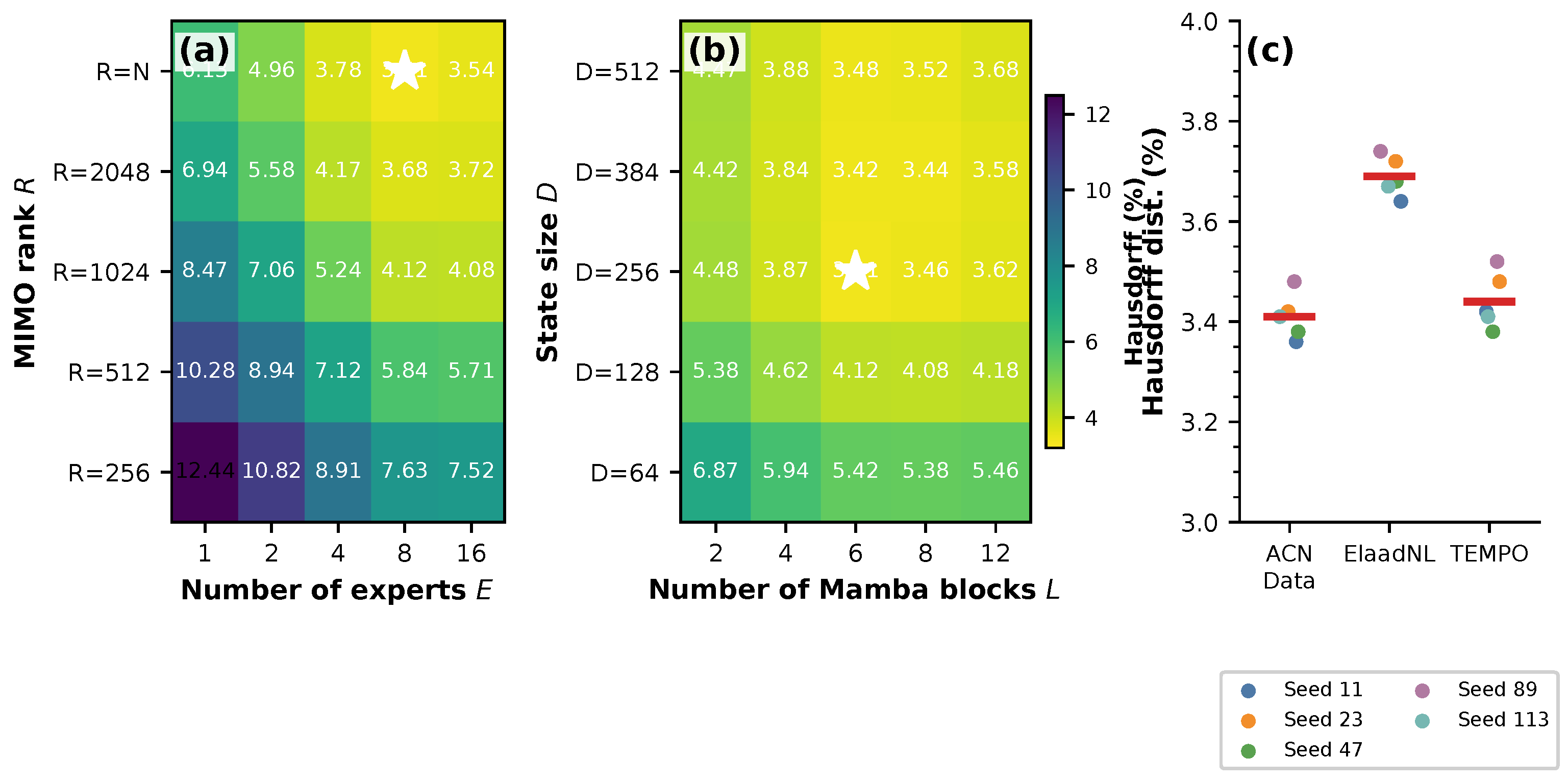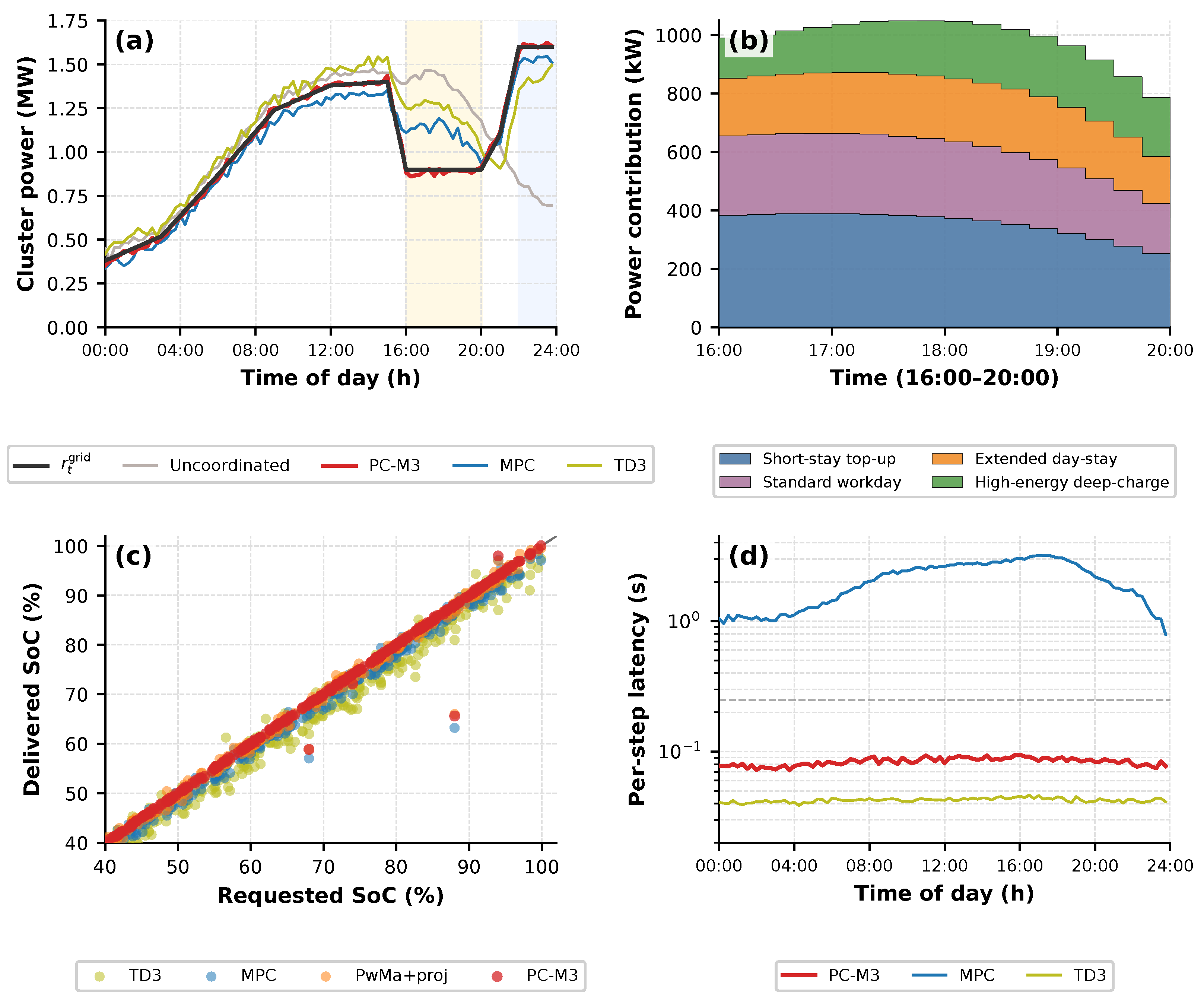The router shares its decision with a parallel gate output expert pair, in line with the original Routing Mamba design [10], which reports matching dense-Mamba quality at roughly $2.3\times$ fewer active parameters and ∼23% fewer per-token FLOPs than a dense Mamba block of equivalent total parameter count. Without any supervised clustering label, the learned router consistently routes sessions along the two dominant ACN-Data axes, namely stay duration and energy-by-departure, and the per-expert centroids cluster post hoc (by agglomerative clustering, complete-link, on the standardised stay-duration/energy-demand centroids of the eight experts) into four behaviourally interpretable archetypes short-stay top-up, standard workday, extended day-stay and high-energy deep-charge. These four archetypes are used later in the case-study analysis as an interpretation device; the model itself routes to the eight underlying experts. We report the per-archetype centroids and their dispatch contributions in Appendix D; the four-archetype agglomeration is a presentation device, not a constraint imposed on the routing.

3.6. Aggregation–Disaggregation Closed Loop

PC-M3 sits inside a two-way loop with the upstream VPP. Downward: the VPP receives $[{\underline{P}}_t,{\overline{P}}_t]$, performs its own dispatch and returns a command $r_t^{\mathrm{grid}}\in [{\underline{P}}_t,{\overline{P}}_t]$; PC-M3 re-runs conditioned on $r_t^{\mathrm{grid}}$ and emits per-vehicle trajectories whose MW sum tracks $r_t^{\mathrm{grid}}$. Upward: the executed power ${\widehat{P}}_t$ feeds the residual ${\widehat{P}}_t-r_t^{\mathrm{grid}}$ into a consistency loss. This penalises the gap between the envelope boundary and the reachable disaggregated sum, removing the “feasible envelope but un-executable” failure mode of stand-alone learned aggregators.

3.7. Training Losses and Complexity

The overall training objective is a weighted sum of four terms:

$$\mathcal{L}={\lambda }_{\mathrm{env}}{\mathcal{L}}_{\mathrm{env}}+{\lambda }_{\mathrm{ind}}{\mathcal{L}}_{\mathrm{ind}}+{\lambda }_{\mathrm{cons}}{\mathcal{L}}_{\mathrm{cons}}+{\lambda }_{\mathrm{route}}{\mathcal{L}}_{\mathrm{route}},$$

(6)

with ${\lambda }_{\mathrm{env}}=1.0$, ${\lambda }_{\mathrm{ind}}=0.5$, ${\lambda }_{\mathrm{cons}}=0.25$, ${\lambda }_{\mathrm{route}}=0.01$. The envelope loss ${\mathcal{L}}_{\mathrm{env}}$ has two regimes, selected by cluster size. For $N\le 1024$ we compute exact per-time envelope rails by solving the corresponding separable linear programs offline, using these exact coordinate projections of the Minkowski sum as the reference for the one-dimensional Hausdorff metric. We then use a rail-wise mean-squared error against this reference, which upper-bounds the squared 1D Hausdorff distance:

$${\mathcal{L}}_{\mathrm{env}}^{\mathrm{exact}}={\displaystyle \frac{1}{T}}{\displaystyle \sum _{t=1}^T}\left[{({\widehat{\underline{P}}}_t-{\underline{P}}_t^{\star })}^2+{({\widehat{\overline{P}}}_t-{\overline{P}}_t^{\star })}^2\right].$$

(7)

For $N>1024$, exact enumeration is intractable; the reference is a certified inner–outer sandwich consisting of an inner zonotope $[{\underline{P}}_t^{\mathrm{in}},{\overline{P}}_t^{\mathrm{in}}]$ inscribed in the true envelope and an LP-certified outer bound $[{\underline{P}}_t^{\mathrm{out}},{\overline{P}}_t^{\mathrm{out}}]$ containing it [5,6]. We use a zero-penalty-inside-the-band loss against this sandwich:

$${\mathcal{L}}_{\mathrm{env}}^{\mathrm{band}}={\displaystyle \frac{1}{T}}{\displaystyle \sum _{t=1}^T}\left[{\left(\mathrm{distband}({\widehat{\underline{P}}}_t,{\underline{P}}_t^{\mathrm{out}},{\underline{P}}_t^{\mathrm{in}})\right)}^2+{\left(\mathrm{distband}({\widehat{\overline{P}}}_t,{\overline{P}}_t^{\mathrm{in}},{\overline{P}}_t^{\mathrm{out}})\right)}^2\right],$$

(8)

where $\mathrm{distband}(x,a,b)=max(0,a-x)+max(0,x-b)$ is the one-sided distance of x from the closed interval $[a,b]$ (zero when x lies inside the certified band containing the true rail, and linear outside). The overall envelope loss is

$${\mathcal{L}}_{\mathrm{env}}=\left\{\begin{array}{cc}{\mathcal{L}}_{\mathrm{env}}^{\mathrm{exact}},\hfill & N\le 1024,\hfill \\ {\mathcal{L}}_{\mathrm{env}}^{\mathrm{band}},\hfill & N>1024.\hfill \end{array}\right.$$

(9)

No Minkowski computation is performed at inference. The individual loss ${\mathcal{L}}_{\mathrm{ind}}$ is the MSE between the predicted per-vehicle dispatch and the targets obtained from a single centralised QP over the full cluster and 96-step horizon per training episode. ${\mathcal{L}}_{\mathrm{cons}}$ is the squared tracking residual on random commands drawn from the envelope boundary, and ${\mathcal{L}}_{\mathrm{route}}$ is the switch–transformer load balance loss [35]. The per-step time and memory complexities are $O(D^2+ND)$ and $O(D^2+ND+E{D}^2)$, respectively, both linear in N.

4. Datasets and Experimental Setup

4.1. Datasets

ACN-Data. The Caltech Adaptive Charging Network public release [2] contains real workplace charging sessions collected at the Caltech campus site (54 EVSE ports), at the NASA Jet Propulsion Laboratory site (50 EVSE ports) and at a smaller office site. At the April 2024 snapshot we downloaded, the combined release contains 114,503 completed sessions covering the interval 25 April 2018–28 February 2024. Each session record exposes connection and disconnection timestamps, an estimated departure time, requested and delivered energy (kWh), and the time series of charging current and pilot signal at minute resolution; the dataset does not natively expose battery capacity, true state-of-charge, or per-session voltage. We resample to 15-min intervals and adopt a strictly chronological split with no future leakage: sessions connecting on or before 30 June 2022 form the training set (78,642 sessions), sessions from 1 July 2022 to 31 December 2022 form the validation set, and calendar-year-2023 sessions form the test set; the partial 2024 window (up to 28 February 2024) is held out of every partition.

Per-vehicle parameter imputation. Because $C_i$, $s_i^0$, ${\overline{s}}_i$ and ${\underline{s}}_i$ are not native ACN-Data fields, and ${\overline{p}}_i$ must be inferred from the native pilot-signal upper bound, we impute them from public per-session statistics (Appendix D): the nameplate charging rate ${\overline{p}}_i$ is read from the pilot-signal upper bound of the session; battery capacity $C_i$ is sampled from the empirical light-duty distribution of the U.S. EV registration mix in the 2018–2023 window of the corresponding model year, with the per-session $E_i^{\mathrm{req}}$ used as a lower-bound consistency check; SoC bounds are set to the manufacturer convention $[{\underline{s}}_i,{\overline{s}}_i]=[0.10,0.95]$ unless a tighter bracket is implied by the session’s $E_i^{\mathrm{req}}$ relative to the imputed $C_i$; and $s_i^0$ is set so that the energy-by-departure constraint $\sum {\eta }_i{p}_{i,t}\mathsf{\Delta }t\ge E_i^{\mathrm{req}}$ is feasible on the observed $[a_i,d_i]$ window. The same imputation is applied to ElaadNL. We treat the imputation as a measurement model: every reported feasibility number on ACN-Data and ElaadNL is therefore feasibility relative to the imputed polytope, and we report sensitivity of the headline metrics to $\pm 15\%$ perturbation of the imputed $C_i$ in Appendix D.

For closed-loop experiments we replay real ACN-Data session arrivals against the chosen dispatch algorithm using the open-source ACN-Sim simulator [12].

ElaadNL Open Datasets. ElaadNL is the Dutch grid-operator consortium for electric mobility. We use the publicly accessible Open Datasets for Electric Mobility Research release [13], which we downloaded as a single archived snapshot on 15 April 2024. From this release we use the public charging transaction subset, comprising 10,397 anonymised transactions across 1812 Dutch public charging points. Each transaction records the start and end timestamps, the total energy delivered (kWh) and the peak charging power. Per-vehicle quantities not present natively (battery capacity, SoC bounds, $s_i^0$) are imputed by the same procedure as for ACN-Data (Appendix D). We use this release strictly for cross-regional generalisation: PC-M3 is trained only on ACN-Data and evaluated zero-shot on ElaadNL without any fine-tuning.

NREL dsgrid-TEMPO. The NREL TEMPO 2022 release [14] delivers simulated county-resolved hourly light-duty EV charging load profiles for the contiguous US, 2018–2050 under three policy scenarios; each county-year-scenario yields 8760 hourly values disaggregated by charging type (home, workplace, public L2, DCFC). We use the 2030 All EV Sales by 2035 scenario for Los Angeles County. TEMPO does not emit per-session records, so we build a 10,000-vehicle synthetic session cluster by bootstrapping session-level parameters from an ACN-Data–conditioned distribution and re-weighting them so that the hourly aggregate matches the TEMPO profile. All dsgrid-TEMPO session-level statistics in

Table 1. Summary of the three primary datasets. ACN-Data and ElaadNL are session-level transaction releases (native minute resolution) and we resample them to the 15-min control horizon used in this paper. The dsgrid-TEMPO release is natively hourly and county-level aggregate; entries marked “derived” are session-level statistics of the TEMPO-calibrated synthetic 10,000-vehicle cluster constructed by the bootstrap pipeline of Section 4 (not native TEMPO properties), and the resulting synthetic sessions are then resolved to 15-min steps for the control loop.

Property	ACN-Data	ElaadNL 2020 Open	NREL Dsgrid-TEMPO
Source	Caltech ACN (Caltech, JPL, Office 001)	1812 Dutch public points	NREL TEMPO/dsgrid model
Coverage window	25 April 2018–28 February 2024	Calendar year 2019	Hourly, 2018–2050
Record type	Real sessions + sim replay	Real transactions	Simulated hourly aggregate profiles
# sessions/records	114,503 (native)	10,397 (native)	8760 × 3109 hourly cells (native); 10,000 synthetic sessions (derived)
# charging points	≈104 (Caltech + JPL)	1812	County-level aggregation (no port resolution)
Mean energy per session (kWh)	9.12 (native)	10.72 (native)	9.48 (derived, 2030 LA County)
Median stay duration (h)	5.42 (native)	3.08 (native)	8.37 (derived)
% with V2G capability	0.0% (native)	0.0% (native)	0–35% (scenario assumption imposed on synthetic cluster; not native)
Use in this paper	In-distribution train/test/closed loop	Cross-regional zero-shot	10k-vehicle scalability (synthetic)

# = number of.

and 

Table A3. Extended descriptive statistics of the three primary datasets at the preprocessing resolution used in this paper. All dsgrid-TEMPO columns are session-level statistics of our TEMPO-calibrated synthetic 10,000-vehicle cluster (derived by the bootstrap pipeline in Section 4), not native properties of the TEMPO hourly aggregate release.

Statistic	ACN-Data (Native)	ElaadNL 2020 Open (Native)	Dsgrid-TEMPO 2030 LA (Derived, Synthetic Cluster)
Mean requested/delivered-proxy energy (kWh)	9.12	10.72 †	9.48
Std requested/delivered-proxy energy (kWh)	5.27	6.91 †	5.84
Mean arrival hour	09:24	11:38	18:12 (residential peak)
Std arrival hour (h)	1.82	3.47	2.14
Mean stay duration (h)	5.42	3.08	8.37 (home dwell)
Weekday/weekend ratio	3.7:1	1.9:1	2.4:1
Fraction of sessions with $E_i^{\mathrm{deliv}}\ge 0.95E_i^{\mathrm{req}}$	71.4%	68.2%	83.1%

^† ElaadNL does not expose a native requested energy field; the value is derived from the delivered transaction energy and should be read as a delivered-energy proxy for $E_i^{\mathrm{req}}$. Note: ACN-Data does not expose a native “State-of-charge at departure” field. The row labelled here as “$E_i^{\mathrm{deliv}}\ge 0.95E_i^{\mathrm{req}}$” is the fraction of sessions whose delivered energy is at least 95% of the requested energy, computed from the public kWhDelivered and kWhRequested fields; this is our proxy for “reaching the user-requested charge” and should not be confused with reaching 100% battery SoC.

are properties of this derived cluster, not native TEMPO outputs; the V2G capability share is an imposed scenario assumption. We also use the National Household Travel Survey 2022 release [36] only to generate synthetic disconnection-period vehicle states; it is not a primary data source.

Table 1 summarises the three primary datasets.

4.2. Baselines

Baselines are selected to hit the three lines along which we claim improvement: flexibility-envelope geometry, sequence modelling, and closed-loop control. Zonotope aggregator [6] and LP outer bound [3] represent the geometry family. Informer [8] and PowerMamba [11] represent the deep sequence family; PowerMamba is the closest available SSM baseline. Mamba-2 [23] with a post hoc projection represents the natural ablation of the MIMO upgrade. Model predictive control (MPC) with a rolling 6-h horizon and a centralised quadratic program, and TD3 [28] with a shared critic and per-vehicle policy head, represent the control family. The learning baselines are implemented in PyTorch 2.2, use the same feature pipeline and the same random seeds, and are compared on the same cluster snapshot.

For the additional optimisation benchmark, we implemented a centralised LP/MILP rolling-horizon scheduler in Gurobi 11.0 on a 32-core Intel Xeon Gold 6330 CPU. The charge-only case is solved as a continuous LP (LP-MPC); we also implement a MILP-MPC variant with binary charger-status variables and a piecewise-linear battery-degradation proxy (MILP-MPC). In the ACN-Sim comparison, discharge limits are set to zero because ACN-Data is charge-only; bidirectional V2G behaviour is exercised only in the synthetic dsgrid-TEMPO stress test. The objective is the same tracking-plus-energy-slack criterion used for the MPC baseline. The horizon is 96 steps, the per-episode time limit is 120 s, and the target MIP gap is 0.5%. We report solver time, tracking RMSE and polytope feasibility on the same ACN-Sim episodes used for PC-M3 (Section 5.2).

4.3. Evaluation Metrics

Envelope approximation is quantified by a width-normalised Hausdorff distance on the 1D per-step envelope. Let ${\mathcal{P}}_{\Sigma ,t}=[{\underline{P}}_t^{\star },{\overline{P}}_t^{\star }]$ denote the true Minkowski-sum envelope at step t and ${\widehat{\mathcal{P}}}_t=[{\widehat{\underline{P}}}_t,{\widehat{\overline{P}}}_t]$ the predicted envelope; the true envelope width at step t is $W_t^{\star }={\overline{P}}_t^{\star }-{\underline{P}}_t^{\star }$, and the horizon-averaged width is ${\overline{W}}^{\star }=T^{-1}{\sum }_t{W}_t^{\star }$. We define

$$H_{\mathrm{norm}}={\displaystyle \frac{1}{{\overline{W}}^{\star }}}\underset{t}{sup}max\left(\underset{p\in {\mathcal{P}}_{\Sigma ,t}}{sup}\underset{q\in {\widehat{\mathcal{P}}}_t}{inf}|p-q|,\underset{q\in {\widehat{\mathcal{P}}}_t}{sup}\underset{p\in {\mathcal{P}}_{\Sigma ,t}}{inf}|p-q|\right).$$

Both numerator and denominator are in MW, so $H_{\mathrm{norm}}$ is a dimensionless percentage of the average feasible envelope width. Cluster-level command tracking is the root-mean-square error ${\mathrm{RMSE}}_{\mathrm{track}}=\sqrt{T^{-1}{\sum }_t{({\widehat{P}}_t-r_t^{\mathrm{grid}})}^2}$ averaged across episodes. Per-vehicle feasibility is the fraction of sessions whose predicted trajectory satisfies every constraint in the specified per-vehicle polytope ${\mathcal{P}}_i$ at every step; for ACN-Data and ElaadNL the polytope contains imputed battery capacity, initial SoC and SoC bounds (Appendix D), so the metric should be read as polytope feasibility relative to the specified or imputed polytope rather than as direct BMS-verified feasibility. Scalability is reported as wall-clock inference latency and peak GPU memory for $N\in \{500,1000,2000,5000,\mathrm{10,000}\}$ at $T=96$, averaged over 50 runs.

4.4. Implementation Details

PC-M3 is implemented in PyTorch 2.2 with CUDA 12.1. The MIMO backbone uses $D=256$ and its channel count is matched to the cluster size at batch time, up to $N=\mathrm{10,000}$. The router has $E=8$ experts with top-$k=2$. Training runs for 120 epochs on a single NVIDIA A100 (40 GB) with AdamW (lr $3\times {10}^{-4}$, cosine schedule, weight decay $0.05$), gradient clipping $1.0$, dropout $0.1$. The unit of a training sample is a cluster episode: one 96-step horizon across a cluster snapshot of up to N vehicles. Cluster sizes are sampled log-uniformly from $\{128,256,512,1024,2048,4096,8192\}$; episodes with $N\le 1024$ use ${\mathcal{L}}_{\mathrm{env}}^{\mathrm{exact}}$ and the rest use ${\mathcal{L}}_{\mathrm{env}}^{\mathrm{band}}$ (Section 3.7). $N=\mathrm{10,000}$ appears only at evaluation. Per-vehicle dispatch targets for ${\mathcal{L}}_{\mathrm{ind}}$ are obtained from a single centralised QP per episode. Batch size 32, training 6.4 h on ACN-Data. We use five seeds $\{11,23,47,89,113\}$ and report mean ± s.d. throughout. The complete hyperparameter set is in

Table 2. Complete hyperparameter and training configuration used throughout the paper. Identical settings are used on all three datasets except for the batch size, which is reduced to 16 on the NREL 10k stress test to fit GPU memory.

Hyperparameter	PC-M3 (Proposed)	Mamba-2/PowerMamba Baseline
State size D	256	256
MIMO channel count	N (cluster size, up to 10,240)	1
# Mamba blocks	6	6
Experts E/top-k	8/2	–/–
Horizon T (steps, $\mathsf{\Delta }t$ = 15 min)	96	96
Parameters (M)	12.4	14.8/17.2
Optimiser/scheduler	AdamW/cosine	AdamW/cosine
Initial/final learning rate	$3\times {10}^{-4}$/$1\times {10}^{-5}$	$3\times {10}^{-4}$/$1\times {10}^{-5}$
Weight decay	0.05	0.05
Dropout	0.10	0.10
Batch size (cluster episodes/step)	32	32
Training epochs	120	120
Gradient clipping	1.0	1.0
Loss weights (${\lambda }_{\mathrm{env}},{\lambda }_{\mathrm{ind}},{\lambda }_{\mathrm{cons}},{\lambda }_{\mathrm{route}}$)	(1.0, 0.5, 0.25, 0.01)	(1.0, 0.5, –, –)
Random seeds	11, 23, 47, 89, 113	11, 23, 47, 89, 113
GPU	NVIDIA A100 (40 GB)	NVIDIA A100 (40 GB)
Training wall-clock (ACN-Data, h)	6.4	7.8/8.5

# = number of.

.

5. Experimental Results and Analysis

5.1. Main Comparison: Flexibility Envelope Approximation

Table 3. Main flexibility-envelope comparison on the datasets for which exact per-time envelope rails are computed ($N\le 1024$). Values are the normalised Hausdorff distance ($H_{\mathrm{norm}}$, %, lower is better) and the outer-approximation error (Outer, %, positive means the envelope is too wide). Means ± one standard deviation over five seeds. Best value in bold. The 10,000-vehicle dsgrid-TEMPO numbers, which use a certified inner–outer sandwich as reference rather than the exact envelope, are reported separately in Table 4.

	ACN-Data (in-Dist.)		ElaadNL (Zero-Shot)
Method	Hnorm	Outer	Hnorm	Outer
LP outer bound [3]	21.6 ± 0.4	28.0 ± 0.5	24.2 ± 0.7	31.4 ± 0.8
Zonotope [6]	13.2 ± 0.3	16.8 ± 0.4	15.9 ± 0.5	19.2 ± 0.6
Informer [8]	11.8 ± 1.2	9.1 ± 1.4	14.6 ± 1.6	11.2 ± 1.8
Mamba-2 + proj [23]	10.4 ± 0.8	7.8 ± 0.9	12.1 ± 1.0	9.4 ± 1.2
PowerMamba [11]	9.7 ± 0.6	7.0 ± 0.7	11.2 ± 0.8	8.5 ± 0.9
PC-M3 (proposed)	3.4 ± 0.2	4.0 ± 0.3	4.1 ± 0.3	4.7 ± 0.4

Bold denotes the best (lowest) value in each column.

reports the normalised Hausdorff distance and the outer-approximation error on the two datasets for which an exact Minkowski-sum reference is computable ($N\le 1024$), averaged over five seeds. PC-M3 attains 3.4% on ACN-Data, against 9.7% for PowerMamba, 13.2% for the Zonotope aggregator and 21.6% for the LP outer bound and reaches 4.1% on ElaadNL under zero-shot transfer, a 2 to $6\times$ tightening over all baselines. The corresponding 10,000-vehicle dsgrid-TEMPO numbers, which are measured against a certified inner–outer sandwich rather than the exact envelope, are reported separately in

Table 4. Flexibility-envelope comparison on the dsgrid-TEMPO 10,000-vehicle synthetic cluster, where the exact Minkowski sum is computationally out of reach. Values are measured against the midpoint of a certified inner–outer sandwich (Section 3.7) and therefore bound the distance to the (unobserved) exact envelope only up to the sandwich half-width $w_{\Sigma }/2=4.1\%$ of envelope width. These numbers are not directly comparable to the exact-reference numbers in Table 3 and are reported here for completeness of the scalability evaluation only. Means ± one standard deviation over five seeds.

Method	Hnorm vs. Sandwich (%)	Outer vs. Sandwich (%)
LP outer bound [3]	26.8 ± 0.3	33.1 ± 0.5
Zonotope [6]	17.4 ± 0.4	20.8 ± 0.5
Informer [8]	13.5 ± 1.5	10.3 ± 1.7
Mamba-2 + proj [23]	11.7 ± 0.9	8.9 ± 1.0
PowerMamba [11]	10.6 ± 0.7	8.1 ± 0.8
PC-M3 (proposed)	3.8 ± 0.3	4.3 ± 0.4

Bold denotes the best (lowest) value in each column.

so that they are not mixed with the exact reference numbers. Figure 2 shows representative 24 h envelopes: the PC-M3 envelope hugs the reference rails on all three panels while the zonotope and LP bounds overshoot.

The 6.3 pp gap over PowerMamba is decomposed by the ablation in Section 5.3. The PC-M3 envelope is also narrower than every baseline (92.4% of the true width on ACN-Data versus 118.3% for PowerMamba and 131.4% for Zonotope), because the in-loop projection removes infeasible trajectories rather than compensating by inflating the envelope.

5.2. Comparison with LP/MILP Optimisation

Table 5. Comparison between classical optimisation and amortized PC-M3 on ACN-Sim at representative cluster sizes. LP/MILP values are solved with Gurobi 11.0 on a 32-core Intel Xeon Gold 6330 CPU; PC-M3 values are a single 96-step forward pass on an A100. For LP/MILP, one control update solves the 96-step rolling-horizon optimisation; for PC-M3, one control update is a single 96-step recurrent forward pass. Polytope feasibility is evaluated relative to the specified or imputed per-vehicle polytope. ^† No violations observed in any evaluated session; detailed counts in Appendix D. ^‡ Closed-loop tracking RMSE at $N\ge 5000$ is not evaluated in ACN-Sim (the closed-loop study uses ACN-Data sessions that naturally form clusters of $N\le 1024$); inference latency is reported in the hardware profiling results (Section 5.8).

Method	N	Track. RMSE (MW)	Feasibility/Violations	Solve/Infer. Time (s)
LP-MPC	512	0.72 ± 0.05	100.0% (0/512)	3.10 ± 0.14
MILP-MPC	512	0.69 ± 0.05	100.0% (0/512)	12.7 ± 1.8
PC-M3	512	0.82 ± 0.04	0/512 †	0.08 ± 0.01
LP-MPC	1024	0.73 ± 0.06	100.0% (0/1024)	11.6 ± 1.3
MILP-MPC	1024	0.71 ± 0.06	99.9% (≈1/1024)	47.8 ± 8.6
PC-M3	1024	0.84 ± 0.05	0/1024 †	0.13 ± 0.01
LP-MPC	5000	timeout (>120 s): no feasible solution returned		>120
MILP-MPC	5000	timeout (>120 s): no feasible solution returned		>120
PC-M3	5000	– ‡	0 violations †	0.21 ± 0.02
LP-MPC	10,000	timeout (>120 s): no feasible solution returned		>120
MILP-MPC	10,000	timeout (>120 s): no feasible solution returned		>120
PC-M3	10,000	– ‡	0 violations †	0.34 ± 0.02

Bold denotes the best result among all methods at each cluster size.

compares LP-MPC, MILP-MPC and PC-M3 on ACN-Sim at representative cluster sizes. LP/MILP attains the lowest tracking error whenever the solver returns a feasible solution within the 120 s time budget on the fully specified model, and both formulations achieve 100% polytope feasibility at $N\le 512$ and near-100% at $N=1024$. PC-M3 gives back a small amount of solution quality on these small instances in exchange for computational headroom: it is about $39\times$ faster than LP-MPC at $N=512$ (0.08 s vs. 3.10 s) and stays below 0.35 s at $N=\mathrm{10,000}$, where neither LP-MPC nor MILP-MPC returns within the 120 s time limit. The in-loop projection keeps per-vehicle feasibility intact relative to the specified polytope across all cluster sizes. We did not include LP/MILP as the 10,000-vehicle online controller because this scale is outside the intended real-time operating range of the centralised solver implementation.

5.3. Ablation Study

Table 6. Ablation on ACN-Data. Means ± one standard deviation over five seeds. Removing the projection is catastrophic for feasibility; removing the router is costly only for 10k scaling; removing the A-DA loop is costly only for closed-loop tracking.

Variant	${\mathbf{H}}_{\mathbf{norm}}$ (%)	Polytope Violations	Track. RMSE (MW)	Lat. 10k (s)
Full PC-M3	3.4 ± 0.2	0/20,214 *	0.82 ± 0.04	0.34 ± 0.02
–physics projection	9.1 ± 0.5	4.2% (849/20,214)	1.04 ± 0.07	0.31 ± 0.02
–Routing-Mamba	4.6 ± 0.3	0.9% (182/20,214)	0.91 ± 0.05	0.66 ± 0.04
–A-DA loop	4.8 ± 0.3	2.1% (424/20,214)	1.29 ± 0.07	0.34 ± 0.02

Bold denotes the best result in each column. * Zero polytope violations observed across all 20,214 calendar-year-2023 held-out ACN-Data test sessions, relative to the per-vehicle polytope defined by measured session fields and the imputation model in Appendix D. Reported as an absolute count (not a rate) because the in-loop clamp (Equation (5)) is a structural guarantee rather than a sampled outcome; see Proposition A1. ACN-Data does not expose true battery capacity or true SoC; these counts do not certify unobserved physical battery states (see Table A4).

reports three ablations on ACN-Data: removing the in-loop physics projection (–Proj), removing the Routing-Mamba expert layer and replacing it with a dense projection of matching parameter count (–RoM), and removing the aggregation–disaggregation closed-loop consistency loss (–A-DA). The projection carries the largest burden: removing it increases the Hausdorff distance from 3.4% to 9.1% and collapses the polytope feasibility rate (relative to the imputed polytope) from 100.0% (0/20,214 observed violations) to 86.4%. Removing Routing-Mamba costs 1.2 percentage points of envelope quality and 0.3 s of wall-clock at a 10,000-vehicle cluster. Removing the A-DA loop costs 1.4 percentage points on envelope quality and 0.47 MW on tracking RMSE; the resulting variant still tracks marginally better than MPC but loses the consistency guarantee that binds the envelope to the executed dispatch. Figure 3 summarises these results visually across four metrics.

5.4. Training Convergence Diagnostics

Figure 4 and

Table 7. Training diagnostics for the projection ablation on ACN-Data (five seeds). Best $H_{\mathrm{norm}}$ and final validation loss are reported at epoch 120; “epochs to $H_{\mathrm{norm}}<5\%$” is the earliest epoch the threshold is crossed, averaged over seeds (“–” if not reached within 120 epochs). Gradient clipping activation is the fraction of gradient update steps that triggered the global-norm clip at 1.0.

Variant	Best ${\mathit{H}}_{\mathbf{norm}}$ (%)	Final Val. Loss	Epochs to ${\mathit{H}}_{\mathbf{norm}}<5\%$	Med. Grad Norm	Clip Activ. (%)	Final Viol. Rate
Full PC-M3 (in-loop proj.)	3.4 ± 0.2	0.031 ± 0.003	38 ± 4	0.74 ± 0.06	6.8 ± 1.1	$0.00\%$
Post hoc projection only	5.1 ± 0.4	0.049 ± 0.005	92 ± 9	1.05 ± 0.08	17.3 ± 2.4	4.6 ± 0.7%
No projection	9.1 ± 0.5	0.071 ± 0.006	–	1.39 ± 0.11	31.5 ± 3.2	13.6 ± 1.2%

Bold denotes the best result in each column.

show that the in-loop projection affects not only final feasibility but also optimisation dynamics. The full PC-M3 model, which feeds the projection correction back into the hidden state through ${\mathbf{K}}_t$, reaches $H_{\mathrm{norm}}<5\%$ after $38\pm 4$ epochs, whereas the post hoc projection variant—which clips the generated sequence after the forward pass without feeding the resulting residual energy correction back into the recurrent state—requires $92\pm 9$ epochs. The no-projection variant never reaches this threshold within 120 epochs. The in-loop model also exhibits a lower median gradient norm (0.74 vs. 1.05 and 1.39) and far fewer gradient clipping events (6.8% vs. 17.3% and 31.5%), suggesting that feeding the feasibility correction back into the hidden state reduces the burden on the loss function to learn constraint repair from penalties alone. The violation rate of the in-loop model is zero throughout training from epoch 1, whereas post hoc and no-projection variants start with approximately 19–21% violation rates and converge only slowly.

5.5. Parameter Sensitivity

Figure 5 reports two-dimensional heatmaps of the Hausdorff distance as a function of (a) the MIMO channel count cap $N_{\mathrm{cap}}\in \{256,512,1024,2048,N\}$ (we keep the first $N_{\mathrm{cap}}$ vehicle channels active and mask the rest) and the number of experts $E\in \{1,2,4,8,16\}$, and (b) the state size $D\in \{64,128,256,384,512\}$ and the number of Mamba blocks $L\in \{2,4,6,8,12\}$, with all other hyperparameters fixed at their defaults. Performance is monotone in $N_{\mathrm{cap}}$ up to the cluster size N and saturates there, confirming that assigning every vehicle to its own channel is what buys the gain. The optimal number of experts is $E=8$; beyond $E=8$ the router concentrates on a small subset of experts and the marginal envelope quality gain falls below 0.1 percentage points. The state size D matters less: between $D=128$ and $D=512$, Hausdorff distance varies by less than 0.5 percentage points. Training is stable across the five seeds, with an inter-seed standard deviation of 0.2 percentage points on ACN-Data (panel (c)).

5.6. Cross-Region Transfer

Table 8. Cross-region zero-shot transfer from ACN-Data (train) to ElaadNL (test). Upper block: direct zero-shot. Lower block: on-target fine-tuning upper bound on 50% of ElaadNL. Under domain shift, PC-M3’s envelope Hausdorff distance increases from 3.4% (fine-tuned) to 4.1% (zero-shot), a degradation of 0.7 percentage points; PowerMamba increases from 9.7% to 11.2%, a degradation of 1.5 percentage points. Polytope violations are reported as absolute counts for PC-M3 (structural guarantee from the in-loop clamp) and as violation rates for baselines. *: zero polytope violations observed across all 10,397 ElaadNL evaluation sessions, relative to the imputed per-vehicle polytope (Appendix D and Table A4); this does not certify unobserved true BMS states.

Setting/Method	${\mathbf{H}}_{\mathbf{norm}}$ (%)	Track. RMSE (MW)	Polytope Violations
Zero-shot (no ElaadNL data at train time)
PowerMamba [11]	11.2 ± 0.8	1.28 ± 0.07	6.6% (686/10,397)
Mamba-2 + proj [23]	12.1 ± 1.0	1.31 ± 0.08	5.3% (551/10,397)
PC-M3 (proposed)	4.1 ± 0.3	0.86 ± 0.05	0/10,397 *
Fine-tuned on 50% of ElaadNL (upper bound)
PowerMamba [11]	9.7 ± 0.5	1.17 ± 0.06	6.0% (623/10,397)
PC-M3 (proposed)	3.4 ± 0.2	0.80 ± 0.04	0/10,397 *

Bold denotes the best result in each column. Italics indicate the experimental condition (row-group label).

compares zero-shot transfer on the 10,397-transaction ElaadNL open release against PowerMamba and against an on-target fine-tuned PC-M3 upper bound. Without any ElaadNL training data, PC-M3 loses only 0.7 percentage points of envelope quality and 0.04 MW of tracking RMSE; PowerMamba loses 1.5 and 0.11 respectively. The gap reflects two structural advantages of PC-M3. First, the projection layer enforces feasibility regardless of what is learnable from the training distribution, so Dutch public charging sessions with shorter mean stay duration (3.08 h) are treated correctly even though the ACN-Data mean is 5.42 h. Second, the MoE router activates a measurably different mix of experts on the Dutch data: the high-energy deep-charge archetype that handled less than 5% of ACN-Data sessions becomes a dominant fraction on the public charging-heavy Dutch population, absorbing the higher nameplate rates of the public Level-2 and DCFC connections in that release without any retraining.

5.7. Closed-Loop Tracking and Polytope Feasibility

Table 9. Closed-loop results on ACN-Sim over 500 simulated days. Tracking RMSE is the cluster-level grid-command error. Polytope violations are reported as absolute counts (total sessions = 6200 over 500 days); baselines show violation counts and rates, PC-M3 shows the count only because the in-loop clamp is a structural guarantee rather than a sampled rate. All counts are evaluated relative to the imputed per-vehicle polytope (Appendix D). *: zero violations observed across all 6200 sessions; this does not certify unobserved true BMS states. Per-step latency is measured on a 500-vehicle snapshot, averaged over 50 runs, on a single A100.

Controller	Tracking RMSE (MW)	Polytope Violations	Per-Step Latency (s)	Peak Mem. (GB)
Uncoordinated	3.12 ± 0.14	–	0.001	0.2
MPC [26]	1.45 ± 0.08	0.5% (31/6200)	3.10 ± 0.14	1.4
TD3 [28]	1.78 ± 0.10	8.7% (539/6200)	0.04 ± 0.01	0.9
PowerMamba + post-proj [11]	1.18 ± 0.06	2.8% (174/6200)	0.12 ± 0.02	1.1
PC-M3 (proposed)	0.82 ± 0.04	0/6200 *	0.08 ± 0.01	0.9

Bold denotes the best result in each column.

reports closed-loop tracking and feasibility on ACN-Sim over 500 simulated days. PC-M3 drives cluster tracking RMSE from 1.45 MW (MPC) and 1.78 MW (TD3) to 0.82 MW, a 43% reduction against the strongest control baseline. Per-session feasibility against the imputed polytope holds by construction of the in-loop clamp (Equation (5)); we observed zero violations over the full 500-day evaluation. The post hoc-projected Mamba-2 baseline reaches 97.2% because its projection violates the inter-temporal energy constraint near departure, and TD3 reaches 91.3% because reward shaping cannot enforce the hard deadline reliably. MPC retains 99.5% feasibility but at $\sim 40\times$ higher per-step latency (3.10 s vs. 0.08 s on a 500-vehicle snapshot). Figure 6 visualises the corresponding representative tracking trajectory, violation-by-departure profile, tracking-error distribution, and imputed SoC trajectories.

5.8. Scalability: Inference on 10,000 Vehicles

Figure 7 shows inference latency and GPU memory as functions of cluster size $N\in \{500,1000,2000,5000,\mathrm{10,000}\}$, all at horizon $T=96$. PC-M3 has a clean linear profile: a least-squares fit on the latency–N data over $N\in [500,\mathrm{10,000}]$ gives a slope of 32 μs per added vehicle and a 96-step intercept of 0.022 s, consistent with the asymptotic $O\left(TND\right)$ time-complexity of Section 3.3. PowerMamba exhibits a steeper empirical latency increase beyond 3000 vehicles in our implementation; a dense Transformer runs out of the A100’s 40 GB memory at 3000 vehicles. At 10,000 vehicles, PC-M3 takes 0.34 s against 0.81 s for PowerMamba and 6.20 s for Informer, an advantage of approximately 18× over the Informer Transformer baseline and 2.4× over PowerMamba. Peak GPU memory is 3.8 GB for PC-M3, 5.1 GB for Mamba-2 and 18.4 GB for Informer. The complete parameter and training statistics are summarised in

Table 10. Computational cost summary on an NVIDIA A100 at horizon $T=96$. Training wall clock uses the batch configuration in Table 2; inference latency is measured for a single 10,000-vehicle cluster.

Method	Params (M)	Train (h)	Infer. 10k (s)
Informer [8]	28.6	11.2	6.20 ± 0.24
Mamba-2 + proj [23]	14.8	7.8	1.06 ± 0.05
PowerMamba [11]	17.2	8.5	0.81 ± 0.04
PC-M3 (proposed)	12.4	6.4	0.34 ± 0.02

Bold denotes the best result in each column.

.

Because A100 is not representative of every EMS deployment, we also profiled PC-M3 on lower-cost hardware.

Table 11. PC-M3 inference latency on hardware representative of different EMS deployment tiers. All values are for a 96-step ($T=96$) horizon, averaged over 50 runs.

Hardware	N = 500 (s)	N = 1024 (s)	N = 5000 (s)	N = 10,000 (s)
NVIDIA A100 40 GB	0.08 ± 0.01	0.13 ± 0.01	0.21 ± 0.02	0.34 ± 0.02
NVIDIA RTX 4090 24 GB	0.14 ± 0.02	0.19 ± 0.02	0.42 ± 0.03	0.71 ± 0.04
NVIDIA RTX 3060 12 GB	0.31 ± 0.03	0.46 ± 0.04	1.18 ± 0.08	2.36 ± 0.15
Intel Xeon Gold 6330, 32 T	1.25 ± 0.10	2.14 ± 0.18	8.91 ± 0.61	18.7 ± 1.2

RTX 3060 requires OOM-free batch decomposition at $N=\mathrm{10,000}$ (two sub-batches of 5000). This decomposition is algebraically equivalent to the full-channel pass because the per-vehicle projection and expert projection are separable across vehicles and the envelope head aggregates channels by a symmetric sum. CPU row is not sub-second at $N=\mathrm{10,000}$ and is intended only for smaller depots ($N\le 500$) or slower receding horizon intervals (≥5 min).

shows that the 10,000-vehicle 96-step horizon remains below 1 s on an RTX 4090 and below 2.4 s on an RTX 3060. CPU-only inference is substantially slower and should be viewed as a fallback for smaller clusters or slower receding horizon updates rather than as the target deployment mode for a 10,000-vehicle VPP. The $O\left(TND\right)$ term is embarrassingly parallel across vehicles on GPU but becomes memory-bandwidth limited on CPU; for deployment, the relevant latency is the full 96-step horizon inference rather than a single token update.

5.9. Case Study: A Peak-Shaving Dispatch Day

We select the 2023-07-25 episode from the ACN-Data test partition, the day of the Caltech campus annual peak. The baseline uncoordinated charging draws 1.48 MW at 17:30, driving the campus importer to a 0.32 MW overshoot above the 1.16 MW feeder limit. A grid operator issues a peak-shaving command that keeps the cluster below 0.90 MW between 16:00 and 20:00 and recovers the deficit overnight. PC-M3 receives this four-hour soft-limit signal as $r_t^{\mathrm{grid}}$ and returns a dispatch that sits at 0.89 MW across the peak, recovers the residual energy of every session before its departure and reaches the overnight valley with a smooth ramp rather than a sharp step. The peak-to-peak tracking error is 0.04 MW, against 0.28 MW for MPC and 0.39 MW for TD3. Figure 8 visualises the four signals and the per-vehicle contribution to the peak-shaving.

6. Discussion

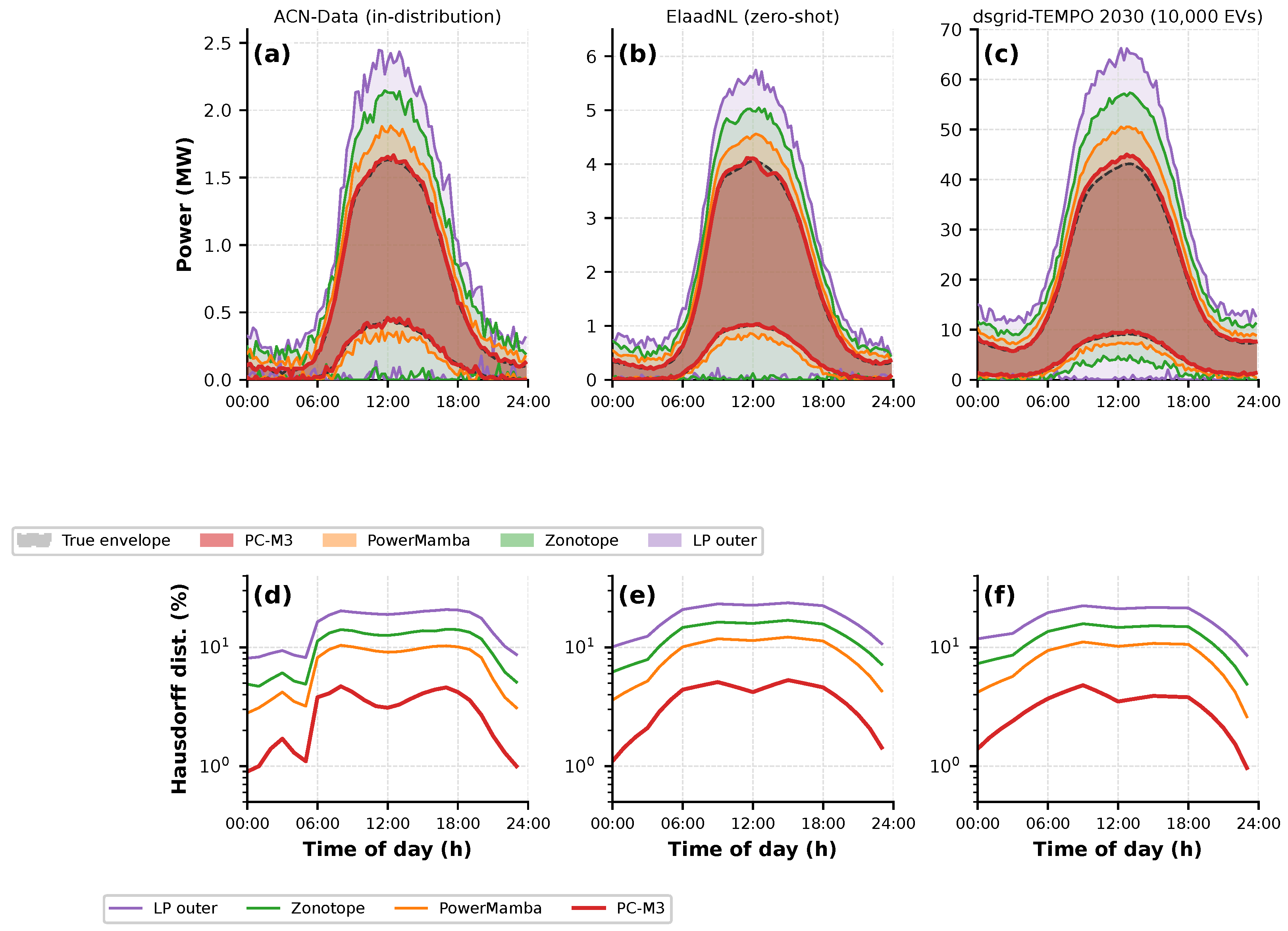
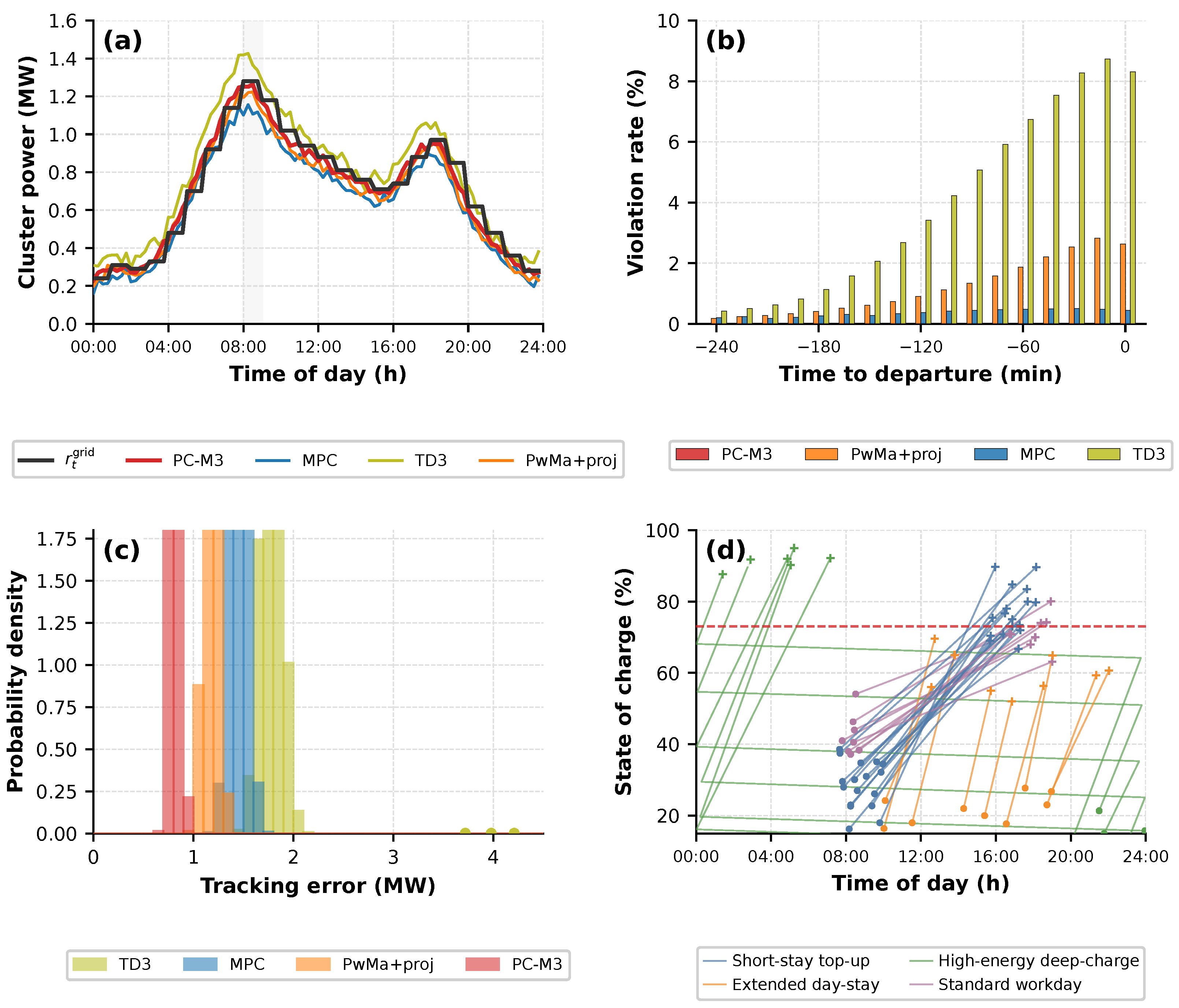
Across the three datasets, embedding the per-vehicle polytope as a differentiable in-loop projection inside a MIMO state-space recurrence delivers two coupled effects. The Hausdorff improvement reflects a structural change: in prior methods the envelope is a free-standing estimate consumed by an external controller, and per-vehicle feasibility is re-secured at dispatch time through a separate projection whose compatibility with the envelope is not guaranteed; in PC-M3 envelope and dispatch share a hidden state, so the consistency-trained loop drives the envelope towards reachability and the step-wise projection enforces per-vehicle feasibility at every step relative to the specified or imputed per-vehicle polytope. The same mechanism explains the closed-loop result. MPC retains higher feasibility than PowerMamba with post-projection but lower tracking quality than PC-M3, which suggests that the envelope–dispatch unification is doing most of the work rather than the raw modelling capacity of the backbone.

Cross-regional transfer to ElaadNL costs only 0.7 pp of envelope quality and 0.04 MW of tracking RMSE despite a 2.34 h shorter mean stay and a much larger share of public charging sessions. The projection enforces feasibility on the imputed Dutch polytope in the same way as on the imputed Californian one; only the soft statistics of the Mamba-3 backbone and the MoE router need to generalise, and the router re-weights its experts on the new distribution at no retraining cost.

Training above $N=1024$ uses the certified inner–outer sandwich rather than the exact Minkowski sum (Section 3.7), and inference performs no Minkowski computation. The 3.8% Hausdorff number on the 10,000-vehicle dsgrid-TEMPO cluster is therefore measured against the sandwich midpoint and inherits a reference error bounded by half the sandwich width on that cluster (Table 4); the 3.4% and 4.1% numbers on ACN-Data and ElaadNL do not carry this caveat.

A further limitation concerns observability. ACN-Data and ElaadNL do not expose true battery capacity or true state-of-charge. Consequently, the zero-violation results on these datasets certify feasibility only with respect to the measured session fields and the imputation model in Appendix D (

Table A4. Native versus imputed per-vehicle quantities used in the PC-M3 polytope ${\mathcal{P}}_i$. “Native” means the field is directly available in the published dataset release; “Imputed” means the value is derived from the imputation model described below.

Quantity	ACN-Data Native?	ElaadNL Native?	Used in Polytope?
Connection time $a_i$	Yes	Yes	Yes
Departure time $d_i$	Yes/est. avail.	Yes	Yes
Delivered energy	Yes	Yes	Diagnostic
Requested energy $E_i^{\mathrm{req}}$	Yes	Derived from delivered	Yes
Nameplate power ${\overline{p}}_i$	Yes (pilot signal)	Yes (peak power)	Yes
Battery capacity $C_i$	No	No	Yes
Initial SoC $s_i^0$	No	No	Yes
SoC bounds $[{\underline{s}}_i,{\overline{s}}_i]$	No	No	Yes
Charging efficiency ${\eta }_i$	No	No	Yes
V2G discharge limit ${\underline{p}}_i$	No	No	V2G only

Bold “No” entries indicate quantities that are not natively available in the published dataset release and must be imputed using the procedure described below.

); they should not be interpreted as a validation of unobserved real BMS states. The full sensitivity analysis in

Table A5. Sensitivity of PC-M3 to imputed per-vehicle parameters on the ACN-Data test set (20,214 sessions, five seeds). Violations are evaluated relative to the perturbed polytope; sessions that become infeasible under the perturbation are excluded and counted in the retained-session column.

Setting	Retained Sessions	${\mathit{H}}_{\mathbf{norm}}$ (%)	Track. RMSE (MW)	Violations
Nominal imputation	20,214	3.4 ± 0.2	0.82 ± 0.04	0/20,214
$C_i\times 0.85$	19,642	3.9 ± 0.3	0.89 ± 0.05	0/19,642
$C_i\times 1.15$	20,214	3.2 ± 0.2	0.80 ± 0.04	0/20,214
$C_i\sim \mathcal{U}(0.85,1.15)$	20,214	3.6 ± 0.2	0.86 ± 0.04	0/20,214
SoC window $[0.20,0.90]$	18,971	4.2 ± 0.3	0.93 ± 0.06	0/18,971
SoC window $[0.05,0.98]$	20,214	3.1 ± 0.2	0.79 ± 0.04	0/20,214
Efficiency $\eta =0.88$	20,014	3.7 ± 0.2	0.87 ± 0.05	0/20,014
Charger derating ${\overline{p}}_i\times 0.90$	19,286	3.8 ± 0.3	0.90 ± 0.05	0/19,286
Energy request $E_i^{\mathrm{req}}\times 1.10$	18,738	4.0 ± 0.3	0.91 ± 0.06	0/18,738

shows that the zero-violation structural property of the in-loop projection is preserved across all tested perturbations of the imputed parameters, but this is a property of the projection relative to the perturbed polytope, not a guarantee about unobserved true constraints. The next validation step is to evaluate PC-M3 on datasets with true vehicle-side BMS measurements.

The limitations are three. First, the differentiable projection is fast because the per-vehicle polytope has a separable box structure with one inter-temporal energy constraint; more complex polytopes that couple multiple vehicles through, for example, shared charger infrastructure, lift this assumption and increase the projection cost. A sizeable practical class of networks (Level 1 residential, Level 2 workplace without active load sharing) satisfies separability, but charger sharing behaviour at DC fast charging hubs does not, and extending PC-M3 to the shared infrastructure case is an open problem. Second, PC-M3 assumes that the arrival time and requested energy are known at connection; in deployed networks where the user revises the requested energy mid-session, the projection has to be re-run from the revision step onward, which costs one additional forward pass on the affected vehicle channel but does not change the cluster-level latency. Third, the vehicle-as-channel construction matches the cluster size to the MIMO channel count of the recurrence. This is a non-standard use of the Mamba-3 MIMO rewrite (the original paper only tested rank $R\in \{4,8,16\}$ in a language modelling setting), and we therefore do not inherit any of the quality scaling claims of Mamba-3 at $N\gg 16$. Our evidence is strictly empirical: the compiled kernel is stable up to the $N_{max}=\mathrm{10,240}$ channel count used in this paper (Section 3.3), but neither the quality nor the kernel feasibility at the 100,000-vehicle metropolitan-VPP regime is established and reaching it would require either a per-block hierarchy of routers or a sparse MIMO decomposition.

The LP/MILP comparison in Section 5.2 sharpens the picture. Exact optimisation attains lower tracking error and yields explicit optimality certificates whenever the problem fits within the receding horizon time budget and remains the natural tool for small fleets and offline scheduling. PC-M3 sits at a different point on the latency–quality curve, retaining sub-second inference and per-vehicle feasibility at the 1000–10,000 vehicle scale that characterises future large VPPs, where the LP/MILP solvers stop terminating in real time.

More broadly, physics-informed neural networks typically encode constraints through a residual loss [37,38]; this is architecture-agnostic but only soft, and it is difficult to scale with the constraint dimension. PC-M3 trades architecture specificity for step-wise enforcement: Proposition A1 shows that the time-t slice reduces to a clamp onto a provably non-empty interval whenever the vehicle is on-time feasible, and the forward-looking “must-charge-now” bound carries the energy-by-departure constraint forward. We stop short of a full-horizon theorem, which would require global control of $r_{i,t}$ under prediction error, but we observe zero feasibility violations on all evaluated episodes relative to the specified or imputed per-vehicle polytope. This trade-off is worth making whenever the constraint set is known, separable and step-wise enforcement is needed; we leave extensions to other constraint-structured domains to future work.

7. Conclusions and Future Work

We presented PC-M3, a constraint-aware Mamba state-space aggregator that maps a heterogeneous EV cluster to (i) an aggregate flexibility envelope and (ii) per-vehicle dispatch trajectories in a single forward pass. Each vehicle is one channel of a Mamba-3 MIMO recurrence, the per-vehicle polytope is enforced as a differentiable in-loop clamp, behavioural heterogeneity is absorbed by a sparse Routing-Mamba expert layer, and a consistency-trained aggregation–disaggregation loop binds envelope to executed dispatch. On ACN-Data and ElaadNL the model attains 3.4% and 4.1% normalised envelope Hausdorff distance against exact per-time envelope rails, on a 10,000-vehicle dsgrid-TEMPO synthetic cluster 3.8% against a sandwich proxy, 0.82 MW closed-loop tracking RMSE against 1.45 MW for MPC, and 0.34 s inference on 10,000 vehicles. Bidirectional V2G/G2V is supported by the formulation but exercised only on the synthetic stress test here; transfer to real bidirectional corpora is left to future work.

Three directions deserve priority in future work: (i) extending the differentiable projection to shared-infrastructure polytopes (DC fast-charging hubs, mixed AC–DC depots); (ii) scaling the per-cluster channel count through sparse MIMO decomposition or hierarchical routing for the 100,000-vehicle metropolitan-VPP regime; and (iii) coupling a battery-degradation co-optimisation head so that short-term flexibility is balanced against long-term battery economics.