Qrisp-Based Implementation and Experimental Evaluation of a T-Count-Optimized Non-Restoring Quantum Square-Root Circuit

Abstract

Efficient quantum arithmetic is a prerequisite for the practical realization of large-scale quantum algorithms, yet many resource-optimized designs remain at the theoretical level. In this work, we present a complete implementation of the T-count-optimized non-restoring quantum square-root circuit proposed by Muñoz-Coreas E. and Thapliyal H. in the Qrisp quantum programming framework. The implemented design follows the garbageless square-root construction based on reversible arithmetic and is built from modular sub-circuits, including reversible adders, subtractors, controlled add/subtract blocks, and controlled adders. We show that the high-level abstractions provided by Qrisp enable a direct and reusable realization of the algorithm while preserving the theoretical resource advantages of the original circuit. To assess practical feasibility, the circuits were additionally executed on IBM’s ibm_marrakesh superconducting quantum processor. The experimental results show that the algorithm can run on contemporary NISQ hardware for small input sizes, although compilation overhead, two-qubit gate errors, readout errors, and relaxation effects significantly reduce success rates as the circuit size increases. Among the tested runtime techniques, dynamical decoupling provided only limited improvement. These results establish the practical realizability of a resource-efficient quantum square-root circuit and provide insight into the challenges of executing arithmetic-heavy quantum algorithms on present-day hardware. These results demonstrate that the previously proposed T-count-optimized non-restoring square-root circuit can be realized as a modular Qrisp implementation, exported to Qiskit, and experimentally evaluated on contemporary NISQ hardware, while also highlighting the practical limitations imposed by compilation overhead and hardware noise.

1. Introduction

Quantum computing has emerged as a paradigm capable of solving certain problems much faster than classical computers. Quantum algorithms use superposition and entanglement to achieve these speedups. For example, Shor’s algorithm [1] for integer factorization runs in polynomial time and is capable of breaking popular cryptographic algorithms such as RSA. Grover’s search, on the other hand, can find a target item in an unsorted database in $O\left(\sqrt{N}\right)$ steps instead of $O\left(N\right)$, which can speed up brute force attacks [2]. More broadly, quantum algorithms have been developed for applications ranging from cryptography to linear algebra and the simulation of physical systems [3,4,5,6]. These advances highlight the potential of quantum computing across diverse fields of science and engineering.

Among the computational tasks that quantum computers will tackle, implementing fundamental arithmetic operations is crucial for enabling larger algorithms. One such operation is the square root, which is common in scientific and engineering computations. Following the discussion in [7], the optimized square-root circuit can decrease the required resource for computing the natural logarithm [8]. The square-root circuit can also be used in the implementation of algorithms computing roots of polynomials [9] or evaluating quadratic congruence [10]. Wang et al. [11] also use a square-root circuit in their quantum Fast Poisson Solver. In their work, the square-root operation is computed with m-qubit precision, where $m=2n+2+f$, and f depends on the required eigenvalue accuracy ${\epsilon }_1$. Accordingly, efficient quantum circuits for functions such as the square root are needed to integrate quantum computing into these applications.

Several quantum circuit designs for square-root operation have been proposed in the literature, each with varying trade-offs between gate count, qubit usage, and garbage output [8,12,13]. One particularly efficient approach is based on the non-restoring square-root algorithm [7]. This algorithm has been shown to produce a quantum circuit with reduced T-count and qubit requirements compared to other square root methods, such as those based on Newton iteration [8]. The design minimizes the usage of the ancilla and avoids garbage production by construction, and its resource efficiency has been analyzed in detail in terms of both gate complexity and fault-tolerant considerations.

In this work, we implement the non-restoring square-root algorithm proposed in [7] using the Qrisp quantum programming framework [14]. Qrisp enables the high-level construction of reversible circuits and offers built-in support for common quantum operations that are used in the implementation of arithmetic components. The modularity and flexibility of Qrisp allow for a direct mapping of the algorithm’s structure into a circuit composed of reusable subcomponents, including reversible addition, subtraction, and conditional logic blocks. Qrisp was chosen for this implementation due to its ability to simplify the design of arithmetic circuits through high-level abstractions, uncomputation, and backend-independent compilation, significantly simplifying the development and analysis of quantum algorithms.

The implementation demonstrates that the algorithm from [7] can be realized in a modern quantum software framework and executed beyond the level of theoretical design. We constructed the circuit in Qrisp, validated its correctness, and evaluated its behavior on actual IBM Quantum hardware under realistic noise conditions. This work shows that resource-optimized arithmetic designs can be translated into executable quantum circuits and experimentally studied on noisy intermediate-scale quantum (NISQ) devices, highlighting the practical limitations imposed by hardware noise, limited connectivity, and compilation overhead.

In the following, we give a roadmap for the remainder of this paper. Section 2 introduces the quantum gates and theoretical concepts required for the construction of the algorithm. Section 3 describes the non-restoring quantum square-root algorithm. Section 4 presents its implementation in the Qrisp framework, including the design of the main arithmetic components. Section 5 provides experimental validation on real quantum hardware and analyzes the obtained results. Finally, Section 6 summarizes the main contributions of this work and outlines directions for future research.

2. Basics

This section briefly introduces selected types of quantum gates and circuits that are needed to describe and build a quantum square-root algorithm.

2.1. T-Depth and T-Count

Let a quantum circuit be expressed on the Clifford + T gate set. Two common cost metrics are the following:

• T-Count: Total number of T gates in the circuit.
• T-Depth: Minimum number of sequential layers of T gates, where gates in the same layer act on disjoint qubits and may be executed in parallel.

These metrics are used because T gates are expensive to implement in fault-tolerant quantum computation. Optimizing for low T-count reduces the total overhead, whereas optimizing T-depth minimizes the circuit runtime. Together, they help assess the practicality of quantum algorithms on real hardware.

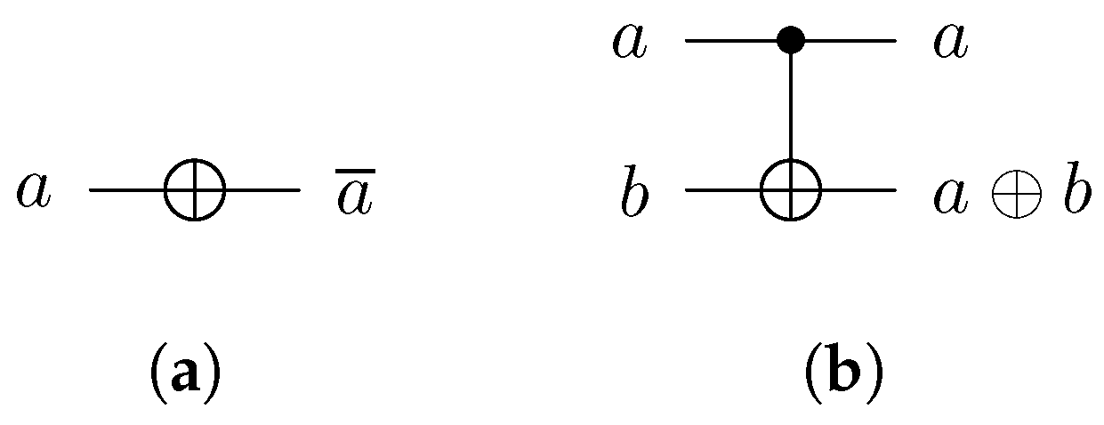
2.2. The NOT Gate

The NOT gate is a single-qubit gate represented as shown in Figure 1a. Since it does not contain T gates, its T-count and T-cost are 0.

2.3. The CNOT Gate

The Controlled-NOT (CNOT) gate is a 2-qubit reversible gate having the mapping for input qubits a and b to output qubits a and $a\oplus b$, respectively. The quantum representation of the CNOT gate is shown in Figure 1b. The T-count and T-cost of the CNOT gate are 0.

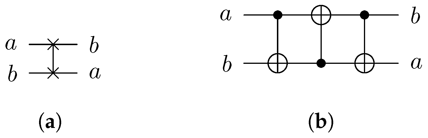
2.4. The SWAP Gate

The SWAP gate is a gate that swaps the states of two qubits. A quantum representation of the gate in a quantum circuit is shown in Figure 2a. It can be broken down into 3 CNOT gates, as shown in Figure 2b. The T-count and T-cost of the CNOT gate are 0.

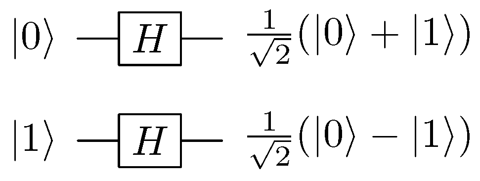
2.5. The Hadamard Gate

The Hadamard gate is a single-qubit gate that maps the state $|0\rangle$ to the superposition state ${\displaystyle \frac{1}{\sqrt{2}}}(|0\rangle +|1\rangle )$ and the state $|1\rangle$ to the superposition state ${\displaystyle \frac{1}{\sqrt{2}}}(|0\rangle -|1\rangle )$. A quantum representation of the Hadamard gate is shown in Figure 3. The Hadamard gate is a Clifford gate; therefore, the T-count and T-depth of the Hadamard gate are 0.

2.6. The T and $T^{†}$ Gates

The T and T^† gates are single-qubit gates that are used to control the phase of a qubit. The T gate is a gate that adds a phase of ${\displaystyle \frac{\pi }{4}}$ to the state, and the T^† gate is a gate that removes a phase of ${\displaystyle \frac{\pi }{4}}$ from the state.

2.7. The Toffoli Gate

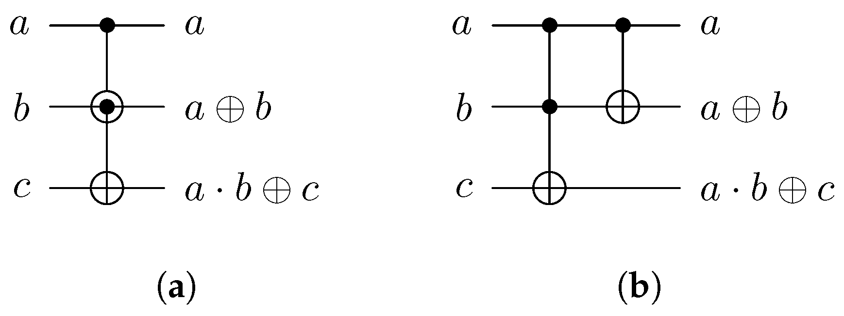
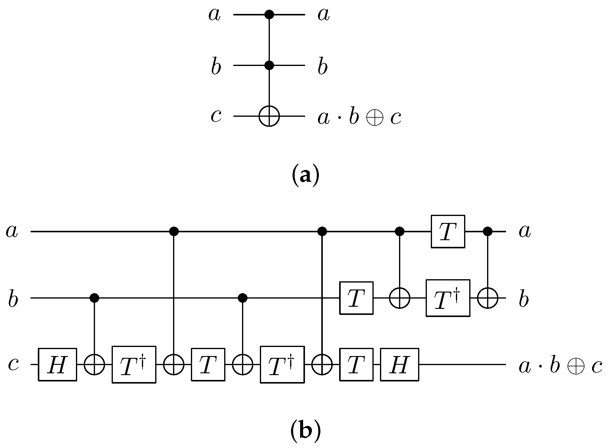
The Toffoli gate is a 3-qubit reversible gate having the mapping for three input qubits $(a,b,c)$ to three output qubits $(a,b,a·b\oplus c)$, as shown in Figure 4a.

One of the Toffoli gate realizations was presented in [15] and is shown in Figure 4b. The decomposition consists of two Hadamard gates, six CNOT gates, four T gates, and four T^† gates. Therefore, the T-count of the Toffoli gate is 7 and the T-depth is 3.

2.8. The Peres Gate

The Peres gate is a 3-qubit reversible gate having the mapping for three input qubits $(a,b,c)$ to output qubits $(a,a\oplus b,a·b\oplus c)$, as shown in Figure 5a. The gate can be constructed from sequentially applied Toffoli and CNOT gates, as shown in Figure 5b. The Peres gate inherits the T-count and T-depth of the Toffoli gate, since the CNOT gate has a T-count and T-depth of 0.

2.9. Addition and Subtraction Circuits

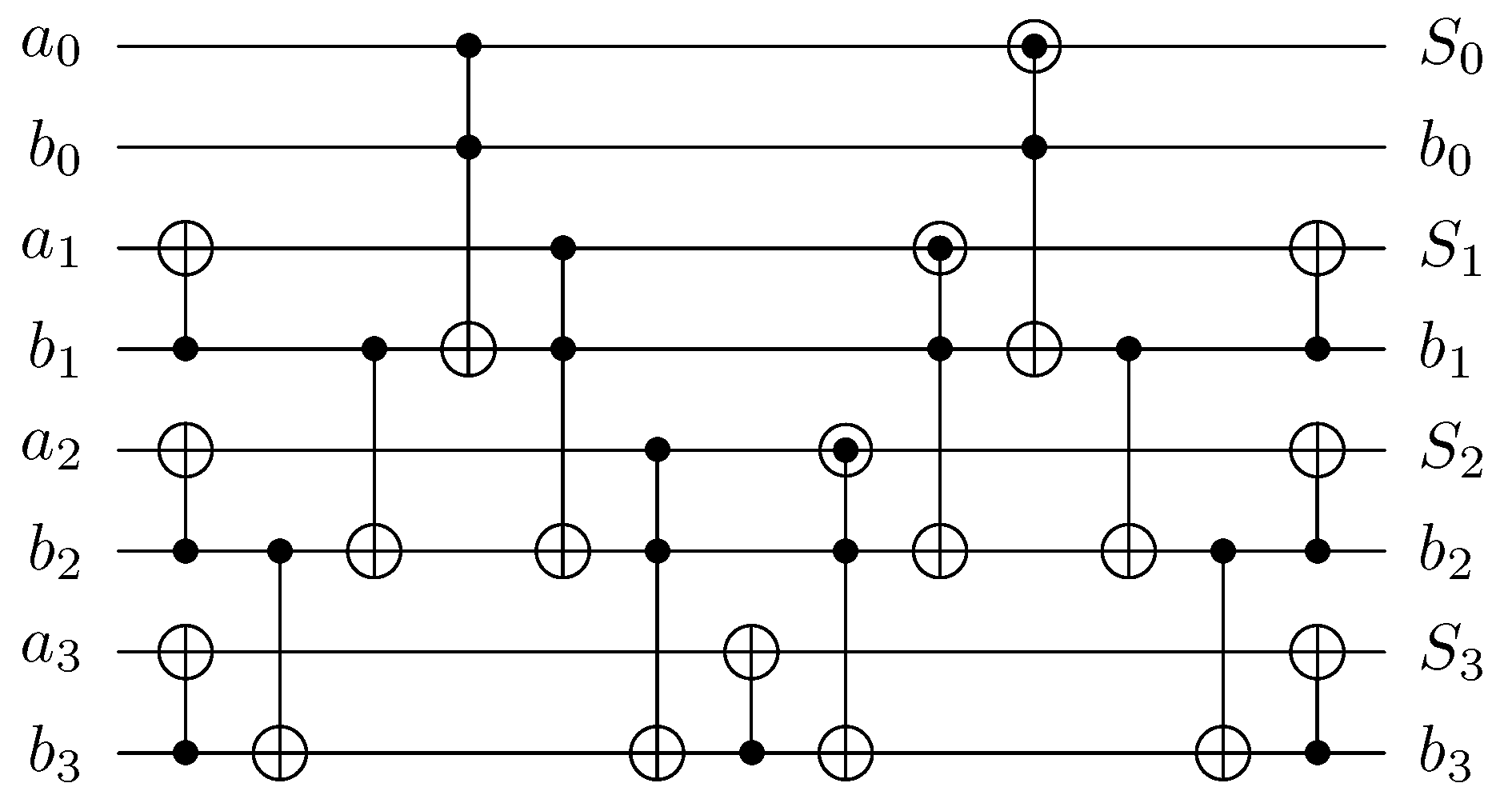
The quantum square-root algorithm described in the next section also requires T-count-efficient addition and subtraction circuits. The addition circuit used in the current implementation follows the idea from [16]. Unlike the original work, this version of the adder omits the overflow qubit. An example of the 4-bit adder is shown in Figure 6.

The implemented reversible ripple carry adder with no ancilla input qubit produces no garbage and places the result of the calculation in the first register. The algorithm follows six steps, described below, for two n-qubits with numbers a and b.

• For $i=1$ to $n-1$:
  Apply the CNOT gate to the qubits $b_i$ and $a_i$, where $a_i$ is the target qubit.
• For $i=n-1$ to 1:
  Apply the CNOT gate to the qubits $b_i$ and $b_{i-1}$, where $b_i$ is the target qubit.
• For $i=0$ to $n-2$:
  Apply the Toffoli gate to the qubits $a_i$, $b_i$, and $b_{i+1}$, where $b_{i+1}$ is the target qubit.
• For $i=n-1$ to 0:
  If $i=n-1$ apply the CNOT gate to the qubits $b_i$ and $a_i$, where $a_i$ is the target qubit (in the original algorithm the Peres gate is applied, but since the overflow qubit is omitted, the CNOT gate is used instead). Otherwise, apply the Peres gate to the qubits $b_i$, $a_i$, and $b_{i+1}$ such that $b_i$, $a_i$, and $b_{i+1}$ are passed to the inputs $a,b,c$ of the Peres gate, respectively.
• For $i=1$ to $n-2$:
  Apply the CNOT gate to the qubits $b_i$ and $b_{i+1}$, where $b_{i+1}$ is the target qubit.
• For $i=1$ to $n-1$:
  Apply the CNOT gate to the qubits $a_i$ and $b_i$, where $b_i$ is the target qubit.

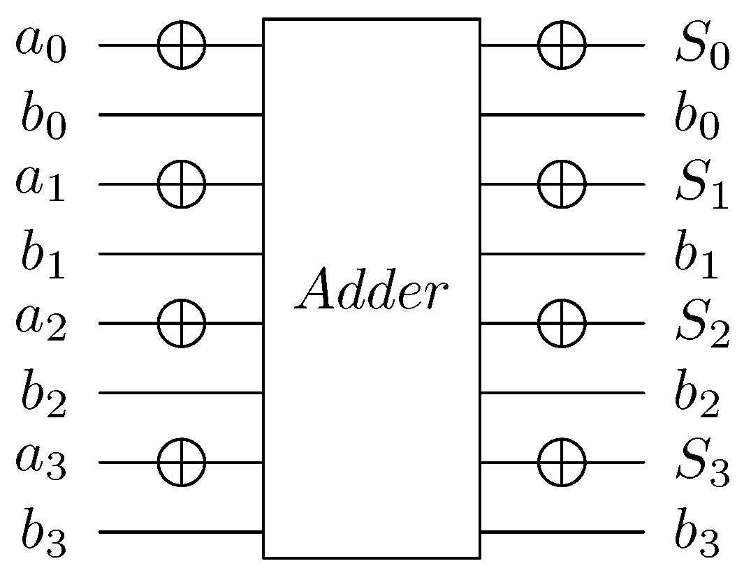
The subtraction circuit utilizes the property that $a-b=\overline{\overline{a}+b}$. Using this property, a subtractor can be designed by inverting the first register, applying the adder, and then inverting the first register again [17]. The example of such a circuit for 4-bit registers is shown in Figure 7.

The T gates are only used in the third and fourth steps of the algorithm and in each step there are $n-1$ Toffoli gates applied. The total T-count then is $(n-1)·7+(n-1)·7$, which can be reduced to $14n-14$. Since the subtractor does not add any additional T gates, the total T-count of the subtractor is $14n-14$ as well.

2.10. Controlled Addition Circuit

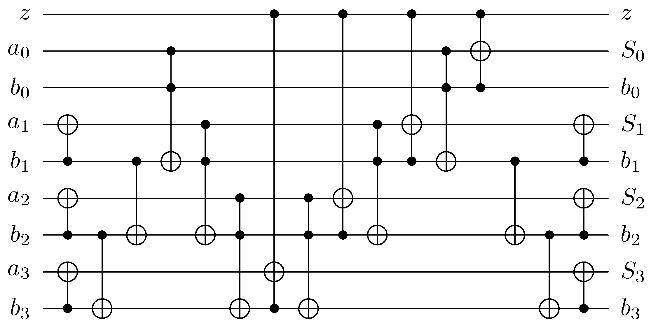
Another arithmetical operation required by the algorithm is T-count-efficient controlled addition. The implemented version of the controlled addition circuit is theoretically described in [18]. Unlike the original work, this version of the controlled adder omits the overflow qubits. An example of the 4-bit controlled adder is shown in Figure 8.

The implemented reversible controlled adder with no ancilla input qubit produces no garbage and places the result of the calculation in the first register. The algorithm follows seven steps, described below, for two n-qubit numbers a and b and control qubit z.

• For $i=1$ to $n-1$:
  Apply the CNOT gate to the qubits $b_i$ and $a_i$, where $a_i$ is the target qubit.
• For $i=n-2$ to 1:
  Apply the CNOT gate to the qubits $b_i$ and $b_{i+1}$, where $b_{i+1}$ is the target qubit.
• For $i=0$ to $n-2$:
  Apply the Toffoli gate to the qubits $a_i$, $b_i$, and $b_{i+1}$, where $b_{i+1}$ is the target qubit.
• Apply the Toffoli gate to the qubits z, $b_{n-1}$ and $a_{n-1}$, where $a_{n-1}$ is the target qubit.
• For $i=n-2$ to 0:
  First apply the Toffoli gate to the qubits $a_i$, $b_i$, and $b_{i+1}$, where $b_{i+1}$ is the target qubit.
  Then, apply the Toffoli gate to the qubits z, $b_i$, and $a_i$, where $a_i$ is the target qubit.
• For $i=1$ to $n-2$:
  Apply the CNOT gate to the qubits $b_i$ and $b_{i+1}$, where $b_{i+1}$ is the target qubit.
• For $i=1$ to $n-1$:
  Apply the CNOT gate to the qubits $b_i$ and $a_i$, where $a_i$ is the target qubit.

The T gates are used in the third, fourth, and fifth steps of the algorithms inside Toffoli gates. In the third step, the total amount of Toffoli gates is $n-1$; in the next step there is one Toffoli gate used. In the fifth step there are $2(n-1)$. The total amount of Toffoli gates is $3n-2$; therefore, the T-count of the circuit is $21n-14$ since the T-count of the Toffoli gate is 7.

3. Quantum Square-Root Algorithm

The quantum circuit presented in [7] calculates the integer square root of a number as well as the remainder utilizing the classical non-restoring square-root algorithm [19]. The proposed circuit is garbageless; it also requires fewer qubits and has a lower T-count compared to the existing designs. Consider a positive binary value a that has an even bit length n. Before computations, three registers are initialized: n-qubit register $|R\rangle$ that contains a, n-qubit register $|F\rangle$ set to 1, and ancilla qubit $|z\rangle$ initialized to 0. Afterwards, the computation register $|R\rangle$ will hold the value of the remainder and the $|F\rangle$ register will contain the integer square root of a for the locations $|F_{n/2-1}\rangle$ through $|F_2\rangle$.

The quantum algorithm is divided into three parts: (1) initial subtraction, (2) conditional addition/subtraction, and (3) remainder restoration.

3.1. Part 1: Initial Subtraction

This part occurs once and contains six steps.

• Apply the NOT gate on the qubit $R_{n-2}$.
• Apply the CNOT gate on the qubits $R_{n-2}$ and $R_{n-1}$ such that $R_{n-1}$ is the target qubit.
• Apply the CNOT gate on the qubits $R_{n-1}$ and $F_1$ such that $R_{n-1}$ is the target qubit.
• Apply the inverted CNOT gate on the qubit $R_{n-1}$ and the ancilla qubit z such that $R_{n-1}$ is the target qubit.
• Apply the inverted CNOT gate on the qubits $R_{n-1}$ and $F_2$ such that $R_{n-1}$ is the target qubit.
• Apply the conditioned ADD/SUB such that qubits $R_{n-4}$ to $R_{n-1}$ make the first argument of the ADD/SUB circuit and qubits $F_0$ to $F_3$ make the second argument, while the ancilla qubit z controls the operation performed.

3.2. Part 2: Conditional Addition or Subtraction

This part occurs $n/2-2$ times for i from 2 to $n/2-1$ and is made of seven steps.

• Apply the inverted CNOT gate on the qubit z and the ancilla qubit $F_1$ such that $F_1$ is the target qubit.
• Apply the CNOT gate on the qubits $F_2$ and z such that z is the target qubit.
• Apply the CNOT gate on the qubits $R_{n-1}$ and $F_1$ such that $F_1$ is the target qubit.
• Apply the inverted CNOT gate on the qubit $R_{n-1}$ and the ancilla qubit z such that z is the target qubit.
• Apply the inverted CNOT gate on the qubits $R_{n-1}$ and $F_{i+1}$ such that $F_{i+1}$ is the target qubit.
• For $j=i+1$ to 3:
  Apply the SWAP gate on the qubits $F_j$ and $F_{j-1}$.
• Apply the conditioned ADD/SUB such that qubits $R_{n-1}$ to $R_{n-2·i-2}$ make the first argument of the ADD/SUB circuit and qubits $F_{2·i+1}$ to $F_0$ make the second argument, while the ancilla qubit z controls the operation performed.

3.3. Part 3: Remainder Restoration

The last part occurs only once and contains nine steps.

• Apply the inverted CNOT gate on the qubits z and $F_1$ such that $F_1$ is the target qubit.
• Apply the CNOT gate on the qubits $F_2$ and z such that z is the target qubit.
• Apply the inverted CNOT gate on the qubits $R_{n-1}$ and z such that z is the target qubit.
• Apply the inverted CNOT gate on the qubits $R_{n-1}$ and $F_{n/2+1}$ such that $F_{n/2+1}$ is the target qubit.
• Apply the NOT gate on the qubit z.
• Apply the controlled addition on the registers R, F, and z such that if the ancilla qubit z has value 1 the R register will hold the value $R+F$ and F will be unchanged. If z is 0, both registers will be unchanged.
• Apply the NOT gate on the qubit z.
• For $j=n/2+1$ to 3:
  Apply the SWAP gate on the qubits $F_j$ and $F_{j-1}$.
• Apply the CNOT gate on the qubits $F_2$ and z such that z is the target qubit.

After the last step, the qubits $|F_{n/2+1}\rangle$ through $|F_2\rangle$ will contain the integer square root of a. And the register $|R\rangle$ will hold the remainder.

4. Implementation in Qrisp

The non-restoring integer square-root algorithm is implemented as a reversible quantum circuit using the Qrisp framework [14]. Each stage of the classical algorithm corresponds to a specific quantum sub-circuit, composed and executed on quantum registers.

First, we need to use the QuantumCircuit(qubit_amount) function, which initiates a circuit with a given number of qubits (qubit_amount) to create a reusable quantum sub-circuit. Then, we can apply operations on the circuit using the append(gate, qubits) function; parameters represent selected gate and indexes of qubits. Known gates like X (NOT gate), CX (CNOT gate), CCX (Toffoli gate), SWAP, etc., can be applied by calling the corresponding methods of QuantumCircuit; for example, qc.x(0) will apply the NOT gate on the first qubit in the circuit. Finally, to build the circuit the to_gate(name) function is used; the resulting gate can be appended to a different circuit.

4.1. Peres Gate

To facilitate arithmetic operations, a three-qubit Peres gate is defined (the introduced gate that combines Toffoli and CNOT gates). The Qrisp code in the peres_gate function constructs this gate by applying a CCX followed by a CX, and converts the circuit into a reusable gate, as shown in Listing 1.

Listing 1. Implementation of the Peres gate.

The Peres gate uses one Toffoli gate and therefore has a T-count of 7.

4.2. Reversible Addition Circuit

Using the Peres gate, an n-bit ripple-carry adder circuit is implemented in the function named add_circuit(n), which returns a reversible gate “ADD” acting on $2n$ qubits. The gate adds two n-qubit numbers, while leaving the second register unchanged and storing the sum $A+B$ in the first register.

The code in Listing 2 follows a six-step operation. The registers A and B are defined as lists of qubit positions, and the comments “Step 1”–“Step 6” correspond to the stages of the addition algorithm described in Section 2.

Listing 2. Implementation of the reversible n-bit ripple-carry adder.

The third step involves $n-1$ Toffoli gates, whereas step 4 uses $n-1$ Peres gates, resulting in a total T-count of $14n-14$.

# <... Preparing the circuit ...> is used to avoid boilerplate code and indicates the part of the code that creates a circuit and defines registers.

4.3. Controlled Addition/Subtraction

Some steps in the non-restoring square-root algorithm require usage of the addition and subtraction operations based on a condition (the sign of the current remainder). These steps are implemented in the ctrl_add_sub_circuit(n) function that constructs a reversible $(2n+1)$-qubit gate, as shown in Listing 3.

Listing 3. Implementation of the controlled addition/subtraction circuit.

The ADD circuit is always applied, and the only thing that changes based on the condition is the sign of the first argument A. This implies that the T-count of the ctrl_add_sub_circuit circuit remains at $14n-14$.

4.4. Controlled Addition

The last step of the original algorithm utilizes the controlled addition circuit to make final adjustments of the arguments based on the remainder’s sign. The implementation of the circuit is located in the ctrl_add_circuit function. If the controlled qubit is 1, the function calculates the sum of the two numbers and places the result in the first register A (the second register remains unchanged); otherwise, both registers stay unchanged. The implementation in Listing 4 follows the seven steps of the described controlled adder.

Listing 4. Implementation of the controlled addition circuit.

The third step uses $n-1$ Toffoli gates, step 4 uses one Toffoli gate, and the fifth step uses $2(n-1)=2n-2$ Toffoli gates. In total, the controlled addition circuit contains $3n-2$ Toffoli gates, which results in a T-count of $21n-14$.

4.5. Initial Subtraction Stage

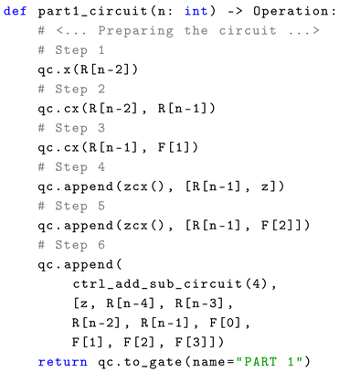
The algorithm begins by an initial subtraction on the most significant bits to establish the first partial remainder. The function part1_circuit(n) returns a $(2n+1)$-qubit operation “PART 1” that prepares the remainder register R and the result register F for the iterative process. The code in Listing 5 shows this initialization step.

Listing 5. Implementation of the initial subtraction stage (PART 1).

The first three steps are implemented using Qrisp functions x(qubit) and cx(ctrl, target) that implement the NOT and CNOT gates, respectively. The fourth and fifth steps require an inverted CNOT operation (zero-controlled CNOT gate) that is implemented by the zcx() function. The function works as a wrapper for the XGate().control(ctrl_state=0) gate. The gate performs the CNOT operation on the target qubit if the control qubit is in state $|0\rangle$. The last step uses the ctrl_add_sub_circuit(4) function that implements the controlled addition/subtraction on the qubits specified in the argument (qubits z, $R[n-4]$ to $R[n-1]$ and $F\left[0\right]$ to $F\left[3\right]$).

Only the sixth step involves T gates due to the use of the controlled addition/subtraction circuit on 4 qubits. Therefore, the T-count of the first part is $14n-14=42$.

4.6. Conditional Addition/Subtraction Stage

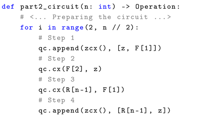
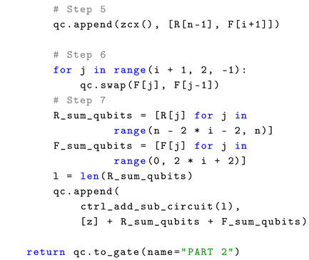
After initialization, the algorithm processes the remaining bits of the input in pairs. The function part2_circuit(n) generates the looped circuit that handles each subsequent pair of bits, using the control logic to decide on addition or subtraction at each step. The pseudocode is essentially a loop that, for each iteration i, prepares the control signals and then applies a controlled add/subtract on an expanding portion of the registers. The implementation is shown in Listing 6.

Listing 6. Implementation of the conditional addition/subtraction stage (PART 2).

First, five steps are implemented in a similar manner as in the previous part. The sixth step uses the swap(q1, q2) function to swap the argument qubits. In the last step, the ctrl_add_sub_circuit() function is appended to the circuit with the control qubit z.

Each iteration i performs controlled addition/subtraction on $2i+2$ qubits, consequently the T-count is $28i+14$. The total T-count can be calculated as ${\sum }_{i=2}^{n/2-1}28i+14={\displaystyle \frac{7}{2}}{n}^2-56$.

4.7. Remainder Restoration Stage

After processing all pairs of bits, the algorithm may end in a state where the last operation was a subtraction, potentially leaving a negative remainder. The final step is to restore a correct non-negative remainder. The function part3_circuit(n) produces a sub-circuit “PART 3” that conditionally adds back the last subtracted value. Its implementation is given in Listing 7.

Listing 7. Implementation of the remainder restoration stage (PART 3).

The operations used in the last part of the algorithm are implemented in a similar way as in the previous parts. The sixth step performs controlled addition on n qubits, which gives a total T-count of $21n-14$.

4.8. Assembling the Square-Root Circuit

The top-level function square_root_circuit(n) composes the full quantum circuit for the integer square root by concatenating the three stages described above. As shown in Listing 8, it simply appends the gates for initial subtraction, the iterative conditional add/subtract, and remainder restoration in sequence on a common set of registers R, F, and z.

Listing 8. Assembly of the full integer square-root circuit (ISQRT).

This assembled gate (named “ISQRT”) acts on $2n+1$ qubits, where n is chosen based on the input size. In our implementation, n is determined as the smallest even number of qubits sufficient to represent the input number a in binary (with two extra bits if needed to accommodate the algorithm’s grouping of bits). The ISQRT circuit can then be applied to quantum registers representing the input and will produce the integer square root in the F register and the remainder in the R register upon measurement.

The total T-count of the implementation can be calculated as the sum of the T-counts of the individual parts of the algorithm. The first part has a T-count of 42, the second part uses ${\displaystyle \frac{7}{2}}{n}^2-56$T gates, and the final part has a T-count of $21n-14$. Thus, the total T-count of the implemented circuit is

$$42+{\displaystyle \frac{7}{2}}{n}^2-56+21n-14,$$

which simplifies to

$${\displaystyle \frac{7}{2}}{n}^2+21n-28.$$

This is equal to the theoretical T-count of the original algorithm reported in [7].

4.9. Executing the Circuit in Qrisp

Finally, to use this circuit within Qrisp, we allocate quantum registers and run a quantum session. Qrisp provides the class QuantumFloat(bit_length, exponent) to represent a n-qubit quantum number and QuantumSession() to simulate circuit execution. The isqrt function as input gets a 2’s complement quantum number R with an even number of qubits and as a result returns the square root of the input and transforms the R register into the remainder.

We prepare two quantum registers: F (result) and z (control flag). Initially, F is set to 1 (as required by the algorithm’s initial conditions), and z to 0. We then append the ISQRT gate to a session and execute it. After execution, the square root is in qubits $F_{n/2+1}$ to $F_2$, so we also need to shift F by 2, to correctly return the square root. The wrapper is given in Listing 9.

Listing 9. Qrisp session wrapper for the integer square-root circuit.

As a result of this function, we obtain a quantum number whose value is the square root. Meanwhile, the input parameter R, which originally held the square, now carries the remainder of the computation. Since the input quantum number R can represent a superposition of multiple values, the resulting output registers (F and R) will also be in a corresponding superposition of square roots and remainders. This property reflects the inherently parallel nature of quantum computation.

In summary, the described implementation in Qrisp provides a complete quantum circuit for the integer square root using the non-restoring method. Each logical step of the classical algorithm is mirrored by a reversible quantum operation, and the Qrisp framework allows us to combine these into a single coherent quantum circuit (ISQRT) that can be applied and tested on arbitrary input values. The implementation illustrates how high-level quantum programming constructs (such as controlled operations and modular circuit composition) can be used to realize complex arithmetic algorithms on quantum hardware.

5. Experimental Validation and Analysis

To evaluate the practical feasibility of the proposed square-root circuit, we performed experimental validation on real NISQ quantum hardware provided by the IBM Quantum Platform. The objective was to verify whether the implemented non-restoring square-root algorithm can be executed on contemporary superconducting quantum processors and to analyze how hardware noise influences the probability of obtaining the correct result.

The experiments were conducted using IBM Quantum Runtime and the Sampler primitive, which returns measurement distributions for executed circuits. Each instance of the algorithm was compiled into a hardware-compatible circuit, transpiled for the selected quantum processor, and executed multiple times to obtain statistically meaningful output distributions.

5.1. Experimental Setup

Currently, IBM Quantum Platform offers three QPUs (quantum processing units): Marrakesh, Fez, and Kingston, which are available cost-free with execution time limitations. These QPUs belong to the Heron r2 generation of superconducting quantum processors and provide 156 physical qubits [20]. The devices are based on superconducting transmon qubits arranged in IBM’s heavy-hex lattice architecture, which limits qubit connectivity in order to reduce crosstalk and improve the reliability of two-qubit gate operations. As a consequence, logical circuits must be mapped to the hardware connectivity graph using hardware-aware transpilation, which may introduce additional routing operations and increase the circuit depth. The processors operate in the noisy intermediate-scale quantum (NISQ) regime, where gate errors, decoherence, and readout imperfections influence the probability of obtaining correct computational results.

The experiments were executed on the IBM Quantum Marrakesh backend. Although Marrakesh does not exhibit the lowest error rates among the publicly accessible IBM Quantum processors, the observed differences in calibration metrics between available backends remain relatively moderate within the context of the conducted experiments. The backend was therefore selected primarily due to its high availability and suitability for repeated execution within the IBM Quantum infrastructure. The calibration data for 12 March 2026 are shown in

Table 1. Calibration data for IBM Marrakesh.

Metric	Median
$T_1$	179.02 μs
$T_2$	86.58 μs
Readout assignment error	$1.07\times {10}^{-2}$
$P(\mathrm{meas}0\mid \mathrm{prep}1)$	$1.61\times {10}^{-2}$
$P(\mathrm{meas}1\mid \mathrm{prep}0)$	$3.42\times {10}^{-3}$
Identity gate error	$3.00\times {10}^{-4}$
RX gate error	$3.00\times {10}^{-4}$
SX gate error	$3.00\times {10}^{-4}$
X gate error	$3.00\times {10}^{-4}$
Measurement error	$1.07\times {10}^{-2}$
Readout length	2584 ns
Single-qubit gate length	36 ns
CZ gate error (2-qubit couplings)	$2.37\times {10}^{-3}$
RZZ gate error (2-qubit couplings)	$4.72\times {10}^{-3}$
2-qubit gate length	68 ns

.

The implemented square-root algorithm operates on $2n+1$ qubits, where n denotes the number of bits used to represent the input integer. The input number is a signed integer with an even number of bits. Because current quantum processors operate in the NISQ regime and are limited by gate fidelity, coherence times, and connectivity constraints, the experiments were conducted for relatively small input sizes that remain feasible after hardware-aware compilation.

Table 2. Input values used in the evaluation.

Input Value a	Bitstring	Root	Remainder	Expected Output
3	0011	1	2	000010010
4	0100	2	0	000100000
5	0101	2	1	000100001
7	0111	2	3	000100011
9	001001	3	0	0000011000000
16	010000	4	0	0000100000000
23	010111	4	7	0000100000111
31	011111	5	6	0000101000110
32	00100000	5	7	00000010100000111
49	00110001	7	0	00000011100000000
71	01000111	8	7	00000100000000111
127	01111111	11	6	00000101100000110

shows a total of 12 input values tested. For each n, one perfect square, one single-bit number, one Mersenne number, and one randomly chosen number were evaluated. The evaluation aims to provide a representative sample of execution scenarios. The column "Expected Output" represents the expected output register, where the first bit is the ancilla value, which is always 0; the next n bits represents the expected square root, where n is the input size; and the rest is the remainder.

The algorithm was implemented using the Qrisp framework and exported to a Qiskit-compatible quantum circuit for execution on IBM hardware by calling the method to_qiskit() on the Qrisp quantum circuit object. Before execution, each circuit was transpiled for the target backend using a hardware-aware compilation pipeline, the example of such transpilation is shown in Listing 10.

Listing 10. Hardware-aware transpilation with a preset pass manager.

This process included qubit mapping, routing operations required to satisfy hardware connectivity constraints, and circuit optimization aimed at reducing circuit depth and the number of two-qubit gates.

All circuits were executed using the IBM Quantum Runtime environment with the Sampler primitive, which returns measurement distributions for executed circuits. For each tested input value a, the compiled circuit was executed with 10,000 measurement shots, producing a probability distribution over all measured bitstrings corresponding to the values stored in the root and remainder registers.

To study the influence of hardware noise and error suppression techniques, the circuits were executed under multiple runtime configurations. In addition to baseline execution, the experiments were repeated with runtime error suppression mechanisms enabled, including dynamical decoupling and Pauli twirling. These techniques were selected because the implemented square-root circuits become deep after hardware-aware transpilation, which increases their exposure to decoherence, idle-time errors, and accumulated two-qubit gate imperfections. Dynamical decoupling can improve performance by inserting pulse sequences into idle intervals, thereby reducing the accumulation of errors associated with relaxation and dephasing while qubits are waiting for subsequent operations. Pauli twirling can improve performance by randomizing coherent and systematic gate errors, converting them into a more stochastic Pauli-like noise channel that is less likely to accumulate constructively over many circuit layers. In this way, dynamical decoupling mainly targets idle-time decoherence, whereas Pauli twirling targets coherent gate-error accumulation. Comparing these configurations makes it possible to assess whether these complementary error suppression mechanisms increase the probability of measuring the correct root and remainder on NISQ hardware. The example of the configuration is shown in Listing 11.

Listing 11. Sampler configuration with dynamical decoupling and Pauli twirling.

To perform the noise simulation, the high-level Qrisp circuit was first transpiled to the native gate set of the target backend. After transpilation, a Qiskit noise model was constructed from the IBM Marrakesh backend instance. This noise model makes it possible to isolate gate errors, readout errors, and thermal relaxation effects, as well as to perform a full-noise simulation of the target backend. The Aer Simulator was then used to execute the noise simulations, as shown in Listing 12.

Listing 12. Noise-model construction and Aer Simulator execution.

5.2. Evaluated Metrics

To assess the performance of the implemented quantum algorithm on real hardware, several complementary metrics were evaluated. These metrics capture both the structural properties of the compiled circuits and the quality of the obtained measurement results under realistic noise conditions.

The primary structural metrics include circuit depth, total gate count, and the number of two-qubit gates. The comparison between logical and compiled circuits provides a direct measure of the overhead introduced by hardware constraints. In particular, circuit depth and total gate count quantify the temporal and operational complexity of the computation, whereas the number of two-qubit gates is especially important due to their significantly higher error rates compared to single-qubit operations.

Additionally, detailed gate counts were reported for the Qrisp logical circuit, its decomposition into the Clifford+T gate set, and the circuit transpiled to the native gate set of IBM Marrakesh. These counts make it possible to verify the theoretical T-count and provide a clearer overview of how the logical circuit is mapped onto the native superconducting gate set.

The main performance metric is the success rate, defined as the probability of obtaining the correct full-register output state: $P_{\mathrm{success}}=N_{\mathrm{correct}}/N_{\mathrm{shots}},$ where $N_{\mathrm{correct}}$ denotes the number of measurements corresponding to the expected output and $N_{\mathrm{shots}}$ is the total number of circuit executions. This metric directly reflects the practical usability of the algorithm on NISQ hardware and captures the cumulative impact of all noise sources.

To evaluate the impact of qubit relaxation, the ratio between total circuit execution time and the relaxation time $T_1$ is considered. This dimensionless quantity characterizes the exposure of qubits to decoherence during computation. Higher values indicate an increased probability of energy relaxation events occurring before the circuit finishes, particularly affecting idle qubits that remain unused for extended periods.

In addition to absolute success probability, the structure of the output distribution is analyzed using the dominance ratio $R_{\mathrm{dom}}=P_{\mathrm{correct}}/P_{\mathrm{next}},$ where $P_{\mathrm{correct}}$ is the probability of the expected output state and $P_{\mathrm{next}}$ corresponds to the second-most-probable measurement outcome. This metric captures how clearly the correct result stands out from competing erroneous states. Values significantly greater than 1 indicate a well-defined peak in the output distribution, while values close to or smaller than 1 suggest a noise-dominated regime with nearly uniform outcome probabilities.

The effectiveness of noise mitigation techniques relative to the baseline is evaluated by paired improvement metric. For each input value a and calibration window w, the paired improvement was computed as

$$\Delta p_j=p_{\mathrm{mitigation},w}-p_{\mathrm{baseline},w},$$

where $p_{\mathrm{mitigation},w}$ denotes the success rate obtained using a given mitigation technique and $p_{\mathrm{baseline},w}$ denotes the corresponding baseline success rate measured for the same input instance and calibration window. Positive values of $\Delta p_j$ indicate an improvement over the baseline execution, while negative values indicate degraded performance.

To quantify run-to-run variability and assess the statistical significance of the observed improvements, the mean paired improvement across calibration windows was reported together with a 95% Student-T confidence interval.

Multiple noise simulations were performed using gate-only, readout-only, relaxation-only, and full-noise models. The simulations were conducted for selected 4-bit and 6-bit test values across multiple random seeds. This allowed the impact of individual error sources to be analyzed separately and compared with theoretical estimates. Due to the substantial depth and gate count of the transpiled circuit, simulations for 8-bit input values were computationally infeasible within the available resources.

Together, these metrics provide a comprehensive evaluation framework, capturing both the resource overhead introduced by hardware constraints and the resulting impact on computational reliability in the presence of realistic quantum noise.

5.3. Experimental Results

Before executing the circuit under noisy conditions and on real quantum hardware, the correctness of the implementation was first verified using the noiseless simulator provided by the Qrisp quantum session. The circuit was tested for all integer input values a in the range from 0 to $2^{10}$, which corresponds to input bit widths n of 4, 6, 8, and 10. The minimum input bit width required by the circuit design is 4, therefore, the values 0, 1, and 2 were represented using 4-bit registers by padding them with two leading zeros. For each input value, a separate circuit instance was constructed and executed, after which the output registers F, R, and the ancilla register were measured. The measurement result represents a probability distribution over possible values of the root, remainder, and ancilla registers. The value measured in F, representing the possible integer square root, and the value measured in R, representing the possible remainder, were compared against the expected classical values, computed as $\lfloor \sqrt{a}\rfloor$ and $a-{\lfloor \sqrt{a}\rfloor }^2$, respectively. For all tested input values, the noiseless simulation produced the expected root, remainder, and ancilla value with probability $100\%$, where the ancilla register was always measured as 0. This confirms the functional correctness of the implemented circuit before hardware-level noise effects were considered.

Table 3. Compiled circuit characteristics.

a	Qubits	Depth	L. Depth	2q Gates	Gates	L. Gates
3	9	624	164	274	1162	64
4	9	630	164	274	1159	64
5	9	645	164	283	1236	64
7	9	634	164	277	1175	64
9	13	1314	323	674	2747	132
16	13	1349	323	642	2670	132
23	13	1307	323	654	2702	132
31	13	1347	323	669	2760	132
32	17	2296	519	1232	4842	219
49	17	2302	519	1209	4820	219
71	17	2346	519	1231	4861	219
127	17	2198	519	1166	4649	219

presents the characteristics of the compiled quantum circuits after hardware-aware transpilation. The reported metrics are divided into two categories: logical (denoted as “L.”) and physical (compiled). Logical metrics correspond to the original circuit generated at the algorithmic level, prior to any hardware constraints, whereas physical metrics describe the circuit after mapping onto a specific quantum device, including routing and optimization overhead.

The difference between these two representations is substantial. In particular, the circuit depth increases by approximately $3.8\times$–$4.5\times$ after compilation, depending on the input size. Similarly, the total gate count grows by more than an order of magnitude (from roughly $13\times$ to $17\times$). This overhead is primarily caused by limited qubit connectivity, which requires insertion of SWAP operations, as well as additional decomposition of high-level gates into native gate sets.

Overall, the comparison between logical and physical metrics highlights the gap between algorithmic designs and their realization on current quantum hardware. Whereas the logical circuit exhibits relatively moderate resource scaling, the compiled circuit incurs substantial overhead, which grows with the number of qubits and ultimately limits practical execution on NISQ devices.

Table 4. Gate-count comparison of the implemented Qrisp circuit across logical, Clifford + T, and IBM Marrakesh native representations.

(a) Logical gate counts of the Qrisp circuit
$\mathit{n}$	2CX	CX	SWAP	X
4	16	41	3	4
6	32	90	6	4
8	52	153	10	4
(b) T-Count and Clifford + T decomposition gates counts
$\mathit{n}$	T-Count	CX	h	t	tdg	X
4	112	146	32	64	48	18
6	224	300	64	128	96	26
8	364	495	104	208	156	34
(c) IBM Marrakesh native gate counts after transpilation
$\mathit{n}$	CZ	RZ	SX	X
4	317	289	573	7
6	763	588	1385	17
8	1341	959	2419	28

presents detailed gate counts for logical Qrisp gates, as well as for their decomposition into Clifford + T gates and transpilation to the native gate set of ibm_marrakesh for different input sizes.

The theoretical T-count shown in Table 4b is calculated as ${\displaystyle \frac{7}{2}}{n}^2+21n-28$ [7] and matches the total number of T and T^† (“t” and “tdg” columns, respectively) gates. This confirms that the implemented circuit preserves the T-count of the original algorithm.

In superconducting quantum hardware, $R_z$ rotations are typically implemented virtually, by adjusting the reference frame of the qubit rather than applying a physical gate. As a result, $R_z$ gates do not contribute significantly to execution time or error accumulation, despite appearing in large numbers in the compiled circuit.

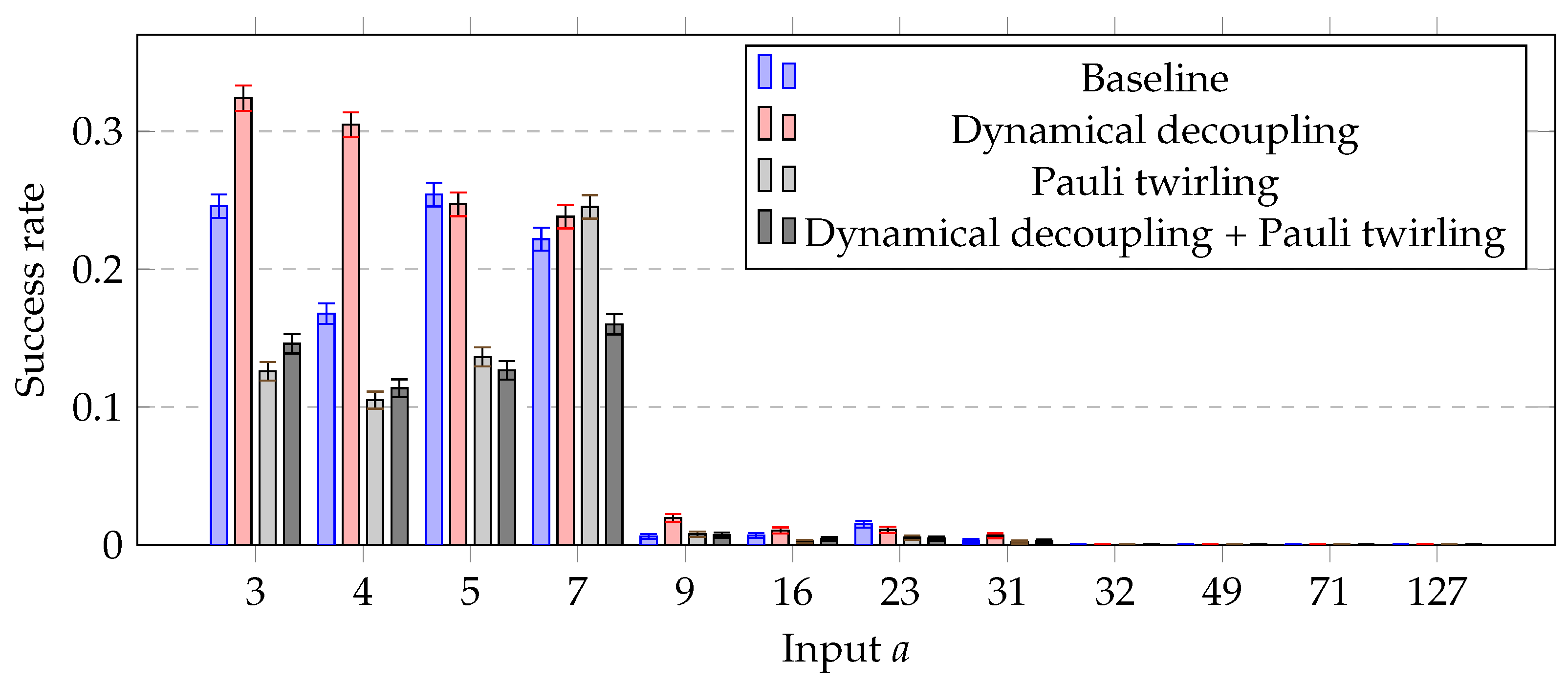
Figure 9 and

Table 5. Success rates for different runtime error suppression techniques. Uncertainties denote 95% Wilson binomial confidence intervals computed from 10,000 measurement shots.

Input a	Baseline	Dynamical Decoupling	Pauli Twirling	DD + PT
3	${0.2457}_{-0.0083}^{+0.0085}$	${0.3240}_{-0.0091}^{+0.0092}$	${0.1259}_{-0.0064}^{+0.0066}$	${0.1459}_{-0.0068}^{+0.0071}$
4	${0.1677}_{-0.0072}^{+0.0075}$	${0.3047}_{-0.0089}^{+0.0091}$	${0.1050}_{-0.0059}^{+0.0062}$	${0.1137}_{-0.0061}^{+0.0064}$
5	${0.2541}_{-0.0084}^{+0.0086}$	${0.2470}_{-0.0084}^{+0.0085}$	${0.1363}_{-0.0066}^{+0.0069}$	${0.1266}_{-0.0064}^{+0.0067}$
7	${0.2217}_{-0.0080}^{+0.0082}$	${0.2380}_{-0.0082}^{+0.0084}$	${0.2451}_{-0.0083}^{+0.0085}$	${0.1600}_{-0.0071}^{+0.0073}$
9	${0.0062}_{-0.0014}^{+0.0017}$	${0.0196}_{-0.0025}^{+0.0029}$	${0.0078}_{-0.0015}^{+0.0019}$	${0.0071}_{-0.0015}^{+0.0018}$
16	${0.0069}_{-0.0014}^{+0.0018}$	${0.0105}_{-0.0018}^{+0.0022}$	${0.0024}_{-0.0008}^{+0.0012}$	${0.0044}_{-0.0011}^{+0.0015}$
23	${0.0150}_{-0.0022}^{+0.0026}$	${0.0110}_{-0.0019}^{+0.0022}$	${0.0053}_{-0.0012}^{+0.0016}$	${0.0046}_{-0.0011}^{+0.0015}$
31	${0.0029}_{-0.0009}^{+0.0013}$	${0.0067}_{-0.0014}^{+0.0018}$	${0.0021}_{-0.0007}^{+0.0011}$	${0.0028}_{-0.0009}^{+0.0012}$
32	${0.0000}_{-0.0000}^{+0.0004}$	${0.0000}_{-0.0000}^{+0.0004}$	${0.0000}_{-0.0000}^{+0.0004}$	${0.0000}_{-0.0000}^{+0.0004}$
49	${0.0001}_{-0.0001}^{+0.0005}$	${0.0001}_{-0.0001}^{+0.0005}$	${0.0000}_{-0.0000}^{+0.0004}$	${0.0000}_{-0.0000}^{+0.0004}$
71	${0.0001}_{-0.0001}^{+0.0005}$	${0.0000}_{-0.0000}^{+0.0004}$	${0.0000}_{-0.0000}^{+0.0004}$	${0.0000}_{-0.0000}^{+0.0004}$
127	${0.0000}_{-0.0000}^{+0.0004}$	${0.0002}_{-0.0001}^{+0.0005}$	${0.0000}_{-0.0000}^{+0.0004}$	${0.0000}_{-0.0000}^{+0.0004}$

show the success rates of the full-register match for the input values tested with different noise mitigation techniques across one calibration window. The success rate drops significantly for larger inputs and approaches 0 for $n=8$. This behavior is expected when deep quantum circuits are executed on NISQ hardware, where the accumulated noise grows with the number of operations and qubits involved. For 4-bit values, dynamical decoupling tends to give a better rate of about $0.28$, against $0.22$, $0.15$, and $0.14$ for baseline, Pauli twirling, and dynamical decoupling + Pauli twirling executions, respectively. However, the effect is not conclusive due to the high variability in results between input values.

The large run-to-run variability is primarily caused by calibration-dependent hardware noise rather than finite-shot uncertainty. The implemented circuit becomes substantially deeper after transpilation and contains hundreds to thousands of two-qubit gates, making the full-register success probability highly sensitive to small changes in qubit mapping, two-qubit gate errors, readout errors, relaxation times, and idle-time structure. Since success requires the exact complete output bitstring, even a small variation in any of these noise sources can produce a noticeable change in the measured success rate.

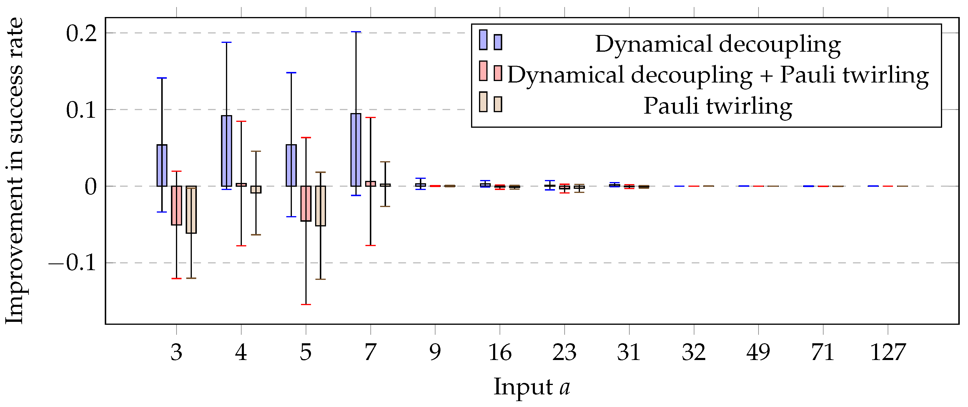
Figure 10 and

Table 6. Paired improvement in success rate relative to baseline execution for different runtime error suppression configurations. Values are reported as mean ± 95% Student-t confidence interval and rounded to three decimal places.

Input a	Dynamical Decoupling	DD + PT	Pauli Twirling
3	$0.054\pm 0.087$	$-0.050\pm 0.070$	$-0.061\pm 0.059$
4	$0.092\pm 0.096$	$0.003\pm 0.081$	$-0.009\pm 0.055$
5	$0.054\pm 0.094$	$-0.045\pm 0.109$	$-0.052\pm 0.070$
7	$0.095\pm 0.107$	$0.006\pm 0.084$	$0.003\pm 0.029$
9	$0.003\pm 0.007$	$0.000\pm 0.001$	$0.000\pm 0.001$
16	$0.003\pm 0.004$	$-0.001\pm 0.003$	$-0.001\pm 0.002$
23	$0.001\pm 0.006$	$-0.003\pm 0.006$	$-0.003\pm 0.005$
31	$0.002\pm 0.003$	$-0.001\pm 0.002$	$-0.001\pm 0.002$
32	$0.000\pm 0.000$	$0.000\pm 0.000$	$0.000\pm 0.000$
49	$0.000\pm 0.000$	$0.000\pm 0.000$	$0.000\pm 0.000$
71	$0.000\pm 0.000$	$0.000\pm 0.000$	$0.000\pm 0.000$
127	$0.000\pm 0.000$	$0.000\pm 0.000$	$0.000\pm 0.000$

illustrate the mean paired improvement in success rate relative to baseline execution for the tested error suppression techniques across five different calibration windows. The results indicate that dynamical decoupling provides the most consistent positive trend among the evaluated techniques. For the smallest input values, the mean improvement obtained with dynamical decoupling is positive, reaching approximately $0.05$–$0.09$ in absolute success probability. However, the confidence intervals for these inputs are relatively large and often cross zero, which means that the observed improvement cannot be regarded as statistically significant at the 95% confidence level. This suggests that dynamical decoupling may be beneficial, but its effect is strongly affected by run-to-run variability.

Pauli twirling alone does not show a consistent improvement over the baseline. For most small input values, the mean paired difference is negative or close to zero, indicating that Pauli twirling either has negligible effect or slightly reduces the probability of obtaining the correct output. The combined use of dynamical decoupling and Pauli twirling also does not consistently outperform dynamical decoupling alone. In most cases, its mean improvement is close to zero or negative, suggesting that the addition of Pauli twirling does not provide a clear advantage for this circuit.

For larger input values, all paired differences converge toward zero. This behavior indicates that, as the circuit size and depth increase, the accumulated effects of gate errors, routing overhead, readout errors, and relaxation dominate the execution. In this regime, the evaluated error suppression techniques are unable to produce a measurable improvement in the success probability. Overall, the paired-difference analysis shows that dynamical decoupling exhibits the most favorable trend, but the large confidence intervals and the near-zero improvements for larger circuits indicate that the mitigation benefit is limited on the tested NISQ hardware.

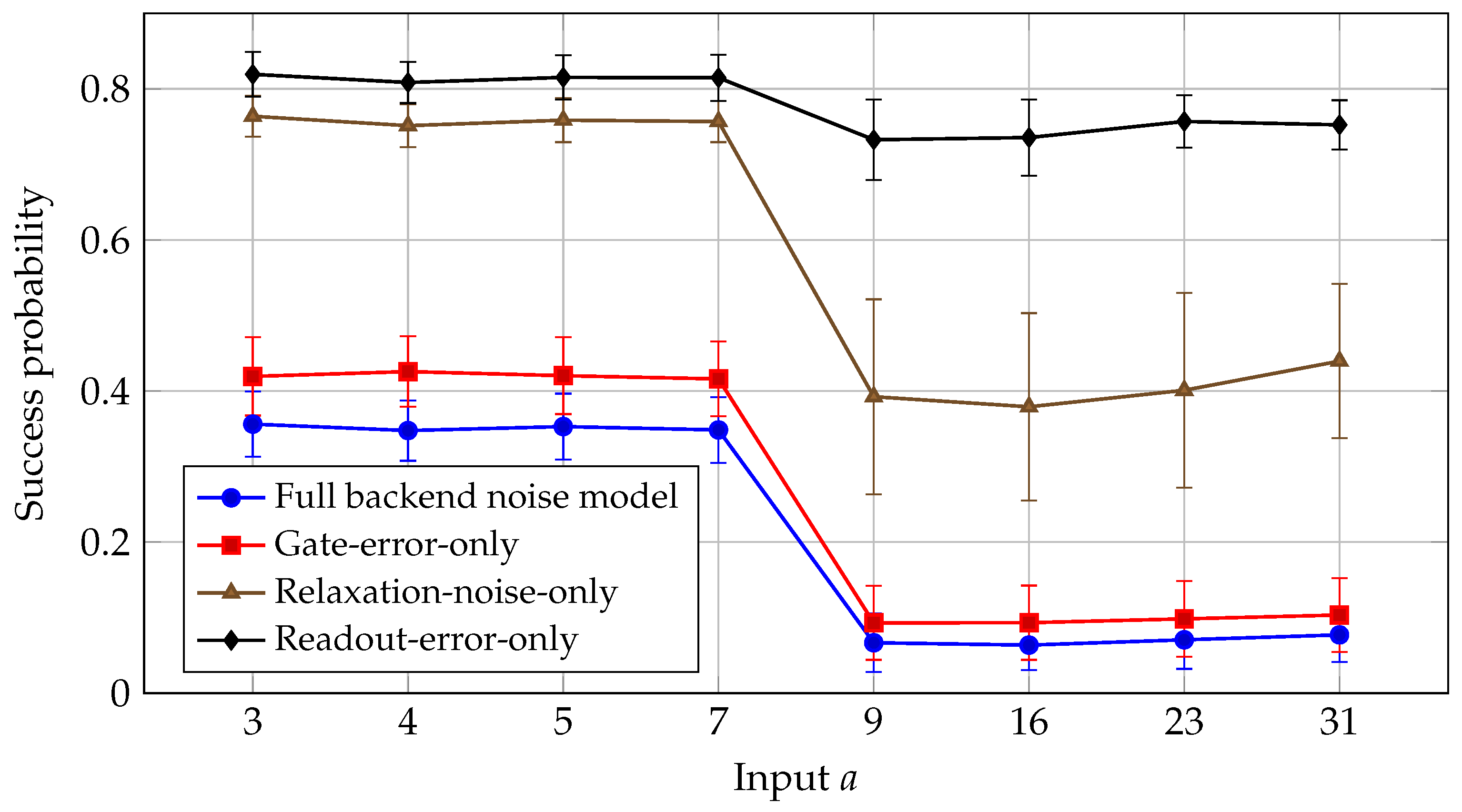
The dominant sources of errors are gate errors, measurement errors, and qubit relaxation during circuit execution. Figure 11 and

Table 7. Comparison of the different noise model simulations. Values are reported as mean ± 95% Student-t confidence interval and rounded to three decimal places.

Input a	Full Noise Model	Gate-Only	Relaxation-Only	Readout-Only
3	$0.356\pm 0.043$	$0.419\pm 0.052$	$0.764\pm 0.027$	$0.819\pm 0.029$
4	$0.348\pm 0.040$	$0.426\pm 0.047$	$0.751\pm 0.028$	$0.808\pm 0.027$
5	$0.353\pm 0.044$	$0.420\pm 0.051$	$0.759\pm 0.029$	$0.815\pm 0.029$
7	$0.348\pm 0.043$	$0.416\pm 0.049$	$0.757\pm 0.027$	$0.815\pm 0.031$
9	$0.067\pm 0.039$	$0.093\pm 0.049$	$0.392\pm 0.129$	$0.733\pm 0.053$
16	$0.064\pm 0.033$	$0.093\pm 0.049$	$0.379\pm 0.124$	$0.736\pm 0.050$
23	$0.071\pm 0.039$	$0.098\pm 0.050$	$0.401\pm 0.129$	$0.757\pm 0.035$
31	$0.077\pm 0.036$	$0.103\pm 0.049$	$0.440\pm 0.102$	$0.752\pm 0.033$

present isolated noise-model simulations for the implemented circuit. The success probability is evaluated as the probability of obtaining the correct full-register output. The four considered cases are the full-backend-noise model, gate-error-only model, relaxation-noise-only model, and readout-error-only model.

In the readout-error-only model, the success probability remains the highest and does not significantly drop for higher input sizes. This is consistent with the fact that readout errors occur only during final measurement and do not accumulate throughout the circuit. If $e_{\mathrm{readout}}$ is the average readout error and $N_m$ is the number of measured qubits, the expected success probability can be approximated as

$$P_{\mathrm{readout}}\approx {(1-e_{\mathrm{readout}})}^{N_m}.$$

Given a median readout error of $0.013$ in the calibration window, we can estimate the readout error as ${(1-0.013)}^9=0.89$ for 4-bit input values and ${(1-0.013)}^{13}$ for 6-bit input values, which is relatively close to the given results.

In the relaxation-noise-only model, the success probability is about $0.75$ for the 4-bit inputs and decreases to approximately $0.40$ for the 6-bit inputs. This indicates that relaxation becomes more significant as circuit duration increases, since qubits remain exposed to $T_1$-related decay for a longer time. However, relaxation noise alone is not sufficient to account for the strongest performance degradation. This may also explain why the improvement obtained from dynamical decoupling is relatively limited: if relaxation is not the dominant error source, suppressing idle-time decoherence would only partially improve the overall success probability, while other errors would continue to contribute substantially to the observed degradation.

In the gate-error-only model, the success probability is approximately $0.42$ for the 4-bit inputs, but drops below $0.10$ for the 6-bit inputs. This sharp decline is caused by the significant increase in the transpiled gate count and circuit depth for $n=6$. Since gate errors accumulate multiplicatively over the sequence of operations, the larger number of gates, especially two-qubit gates, produces a much higher effective failure probability.

In the full-backend-noise model, the success probability is the lowest overall: around $0.35$ for 4-bit inputs and below $0.10$ for 6-bit inputs. Its close agreement with the gate-error-only curve indicates that gate errors are the dominant source of degradation, while relaxation and readout errors provide additional but smaller contributions.

Overall, the simulations show that the circuit is mainly limited by accumulated gate noise after hardware-aware transpilation. Readout errors have a comparatively small effect; relaxation noise becomes more visible for deeper circuits.

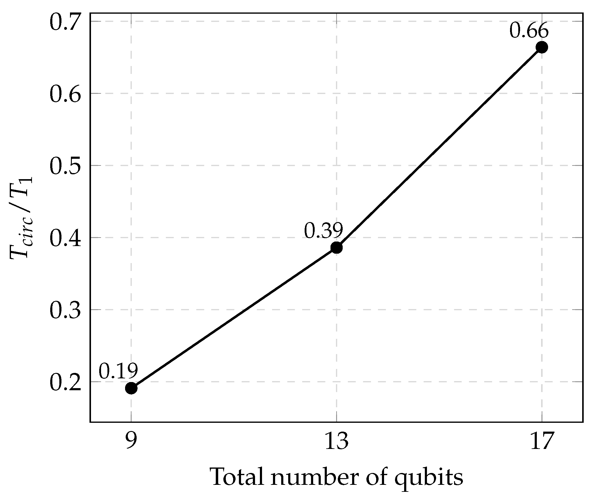
Figure 12 shows the ratio between the total circuit execution time and the qubit relaxation time $T_1$. The ratio starts from approximately $0.19$ for the smallest input values and reaches about $0.66$ for the largest ones. The $T_{\mathrm{circ}}/T_1$ ratio increases with input size because the total depth of the transpiled circuit grows after hardware-aware compilation, extending the circuit execution time and therefore increasing the duration over which qubits are exposed to $T_1$-related relaxation. The increase in the ratio $T_{circ}/T_1$ has important implications for the susceptibility of qubits to decoherence during circuit execution. As the duration of the circuit approaches the characteristic relaxation time $T_1$, the probability that a qubit undergoes energy relaxation before the computation finishes increases significantly. This effect is particularly relevant for qubits that remain idle for substantial portions of the circuit, such as ancillary qubit, which is changed only in specific stages of the algorithm. Although such qubits may participate in relatively few gate operations, they still remain exposed to environmental noise throughout the full execution time of the circuit. This phenomenon highlights an important challenge in NISQ devices: qubits that are logically inactive are still physically evolving and may decohere, which can ultimately affect the reliability of the final measurement outcomes.

Figure 13 shows the dominance ratio $P_{correct}/P_{next}$, where $P_{correct}$ denotes the probability of measuring the expected output state and $P_{next}$ corresponds to the probability of the second-most-probable measured outcome for the baseline execution. The exact numerical values are reported in

Table 8. Dominance ratio between the probability of the correct full-register output state and the probability of the second-most-probable measured state. Values are rounded to three decimal places.

Input Number a	Dominance Ratio
3	3.597
4	5.051
5	7.677
7	3.739
9	1.476
16	2.464
23	3.061
31	2.071
32	0.000
49	0.250
71	0.250
127	0.000

. This metric captures how strongly the output distribution is biased toward the correct solution. For small input values, the ratio is significantly greater than 1, in some cases exceeding 5, indicating that the correct result is clearly distinguishable from competing erroneous states and remains the dominant outcome. As the input size increases, the ratio decreases, reflecting the accumulation of gate errors, readout errors, and relaxation effects in deeper circuits. For intermediate values, the ratio often remains above 1, suggesting that the correct output can still be identified as the most likely measurement outcome despite a reduced absolute success probability. However, for the largest tested inputs, the ratio approaches 0, and the output distribution becomes effectively noise-dominated. In this regime, the probabilities of different outcomes are nearly uniform, indicating that the measured results are close to random and no longer exhibit a meaningful preference for the correct state.

The experimental evaluation demonstrates that the implemented non-restoring quantum square-root circuit is practically executable on current NISQ hardware for small input sizes. The results confirm that the logical design preserves its theoretical efficiency after implementation in the Qrisp framework, while also highlighting a substantial gap between logical and physical circuit representations due to hardware-aware compilation overhead. As observed, the depth of the circuit and the gate count increase significantly after transpilation, leading to a rapid degradation of the success probability with increasing input size. The dominant error sources include two-qubit gate errors, readout inaccuracies, and qubit relaxation effects, which collectively limit the scalability. Among the evaluated error mitigation techniques, dynamical decoupling provides limited improvement, indicating that decoherence during idle periods can be an important factor affecting performance. Overall, the findings validate the feasibility of executing quantum arithmetic circuits on existing devices, while simultaneously emphasizing the need for improved hardware reliability and compilation strategies to enable larger-scale computations.

6. Conclusions

This work translated a previously proposed resource-efficient theoretical design for quantum square-root computation into an executable implementation in the Qrisp framework and examined its behavior under realistic hardware conditions. The study showed that the non-restoring approach can be expressed in a modular way through reversible arithmetic building blocks, allowing the complete circuit to be assembled from reusable components such as adders, subtractors, controlled add/subtract modules, and controlled addition circuits. This confirms that high-level quantum programming environments can be used not only for algorithm prototyping, but also for preserving the structural properties of optimized arithmetic constructions.

From the algorithmic perspective, the implemented circuit retains the main advantages of the design proposed in prior work, namely, the absence of garbage outputs and a low T-count relative to alternative square-root constructions. In particular, the Thapliyal-based non-restoring square-root circuit has a T-count of ${\displaystyle \frac{7}{2}}{n}^2+21n-28$, while the comparable designs considered in the prior evaluation required higher T-counts: $7n^2+14n$ for the design of Sultana et al.; $420n^2+168n-364$ for the design of Bhaskar et al.; ${\displaystyle \frac{21}{4}}{n}^2+{\displaystyle \frac{105}{2}}n-42$ for the first design of AnanthaLakshmi et al.; and ${\displaystyle \frac{21}{4}}{n}^2+{\displaystyle \frac{7}{2}}n-14$ for the second design of AnanthaLakshmi et al. [8,12,13].

The hardware experiments additionally revealed the current execution limits of such arithmetic-heavy circuits on NISQ devices. Although correct results were obtained for small instances, the compiled circuits experienced a substantial increase in depth and gate count after hardware-aware transpilation. This overhead, together with two-qubit gate imperfections, readout errors, and decoherence, rapidly reduced the probability of observing the correct output as the problem size increased. In particular, the results indicate that physical execution costs remain the main obstacle to scaling even theoretically efficient arithmetic circuits on present-day superconducting processors.

Overall, the presented results show that implementing optimized square-root circuits in contemporary quantum software stacks is feasible and that such implementations can be validated on real hardware. The empirical findings are most directly supported for IBM Marrakesh, since all real-hardware executions were performed on this backend. More cautiously, they may be regarded as indicative for closely related IBM Heron r2 devices, such as Fez and Kingston, because these systems share the same processor generation and architectural characteristics. At the same time, quantitative performance should not be assumed to transfer unchanged across devices, since calibration metrics, routing decisions, and backend-specific noise profiles may affect the observed success rates. These results emphasize that progress in compilation methods, qubit connectivity handling, gate fidelity, and error suppression will be essential before larger instances of quantum arithmetic can be executed reliably. The developed implementation can therefore serve as a reference realization of the previously proposed non-restoring square-root circuit, supporting modular circuit construction, Qiskit export, and further experimental studies of arithmetic-heavy quantum algorithms on NISQ hardware.

References

1. Shor, P.W. Polynomial-Time Algorithms for Prime Factorization and Discrete Logarithms on a Quantum Computer. SIAM J. Comput. 1997, 26, 1484–1509. [Google Scholar] [CrossRef]
2. Grover, L.K. Quantum Mechanics Helps in Searching for a Needle in a Haystack. Phys. Rev. Lett. 1997, 79, 325–328. [Google Scholar] [CrossRef]
3. Montanaro, A. Quantum algorithms: An overview. npj Quantum Inf. 2015, 2, 15023. [Google Scholar] [CrossRef]
4. Harrow, A.W.; Hassidim, A.; Lloyd, S. Quantum Algorithm for Linear Systems of Equations. Phys. Rev. Lett. 2009, 103, 150502. [Google Scholar] [CrossRef]
5. Pawlitko, P.; Moćko, N.; Niemiec, M.; Chołda, P. Implementation and Analysis of Regev’s Quantum Factorization Algorithm. arXiv 2025, arXiv:2502.09772. [Google Scholar]
6. Krzyszkowski, J.; Niemiec, M. Analysis of Surface Code Algorithms on Quantum Hardware Using the Qrisp Framework. Electronics 2025, 14, 4707. [Google Scholar] [CrossRef]
7. Muñoz-Coreas, E.; Thapliyal, H. T-count and Qubit Optimized Quantum Circuit Design of the Non-Restoring Square Root Algorithm. J. Emerg. Technol. Comput. Syst. 2018, 14, 36. [Google Scholar] [CrossRef]
8. Bhaskar, M.K.; Hadfield, S.; Papageorgiou, A.; Petras, I. Quantum algorithms and circuits for scientific computing. Quantum Info. Comput. 2016, 16, 197–236. [Google Scholar] [CrossRef]
9. Sun, G.; Su, S.; Xu, M. Quantum Algorithm for Polynomial Root Finding Problem. In Proceedings of the 2014 Tenth International Conference on Computational Intelligence and Security, Kunming, China, 15–16 November 2014; pp. 469–473. [Google Scholar] [CrossRef]
10. van Dam, W.; Hallgren, S. Efficient Quantum Algorithms for Shifted Quadratic Character Problems. arXiv 2000, arXiv:quantph/0011067. [Google Scholar]
11. Wang, S.; Wang, Z.; Li, W.; Fan, L.; Wei, Z.; Gu, Y. Quantum fast Poisson solver: The algorithm and complete and modular circuit design. Quantum Inf. Process. 2020, 19, 170. [Google Scholar] [CrossRef]
12. AnanthaLakshmi, A.; Sudha, G.F. A novel power efficient 0.64-GFlops fused 32-bit reversible floating point arithmetic unit architecture for digital signal processing applications. Microprocess. Microsyst. 2017, 51, 366–385. [Google Scholar] [CrossRef]
13. Sultana, S.; Radecka, K. Reversible implementation of square-root circuit. In Proceedings of the 2011 18th IEEE International Conference on Electronics, Circuits, and Systems, Beirut, Lebanon, 11–14 December 2011; pp. 141–144. [Google Scholar] [CrossRef]
14. Seidel, R.; Bock, S.; Zander, R.; Petrič, M.; Steinmann, N.; Tcholtchev, N.; Hauswirth, M. Qrisp: A Framework for Compilable High-Level Programming of Gate-Based Quantum Computers. arXiv 2024, arXiv:quant-ph/2406.14792. [Google Scholar]
15. Amy, M.; Maslov, D.; Mosca, M.; Roetteler, M. A Meet-in-the-Middle Algorithm for Fast Synthesis of Depth-Optimal Quantum Circuits. IEEE Trans. Comput.-Aided Des. Integr. Circuits Syst. 2013, 32, 818–830. [Google Scholar] [CrossRef]
16. Thapliyal, H.; Ranganathan, N. Design of efficient reversible logic-based binary and BCD adder circuits. ACM J. Emerg. Technol. Comput. Syst. 2013, 9, 17. [Google Scholar] [CrossRef] [PubMed]
17. Thapliyal, H. Mapping of Subtractor and Adder-Subtractor Circuits on Reversible Quantum Gates; Springer: Berlin/Heidelberg, Germany, 2016; Volume 9570, pp. 10–34. [Google Scholar] [CrossRef]
18. Muñoz-Coreas, E.; Thapliyal, H. Quantum Circuit Design of a T-count Optimized Integer Multiplier. IEEE Trans. Comput. 2019, 68, 729–739. [Google Scholar] [CrossRef]
19. Samavi, S.; Sadrabadi, A.; Fanian, A. Modular array structure for non-restoring square root circuit. J. Syst. Archit. 2008, 54, 957–966. [Google Scholar] [CrossRef]
20. IBM. Processor Types. 2026. Available online: https://quantum.cloud.ibm.com/docs/en/guides/processor-types (accessed on 28 March 2026).
Figure 1. NOT (a) and CNOT (b) gates.
Electronics 15 02334 g001
Figure 2. The SWAP gate (a) and it’s decomposition (b).
Electronics 15 02334 g002
Figure 3. The Hadamard gate.
Electronics 15 02334 g003
Figure 4. The Toffoli gate (a) and it’s decomposition (b).
Electronics 15 02334 g004
Figure 5. The Peres gate (a) and it’s decomposition (b).
Electronics 15 02334 g005
Figure 6. Example 4-bit addition circuit.
Electronics 15 02334 g006
Figure 7. Example of 4-bit subtraction circuit.
Electronics 15 02334 g007
Figure 8. Example 4-bit controlled addition circuit.
Electronics 15 02334 g008
Figure 9. Comparison of success rates for different runtime error suppression techniques across one calibration window. Error bars show 95% Wilson binomial confidence intervals computed from 10,000 measurement shots.
Electronics 15 02334 g009
Figure 10. Paired improvement in success rate relative to baseline execution for different runtime error suppression configurations. Error bars show 95% Student-t confidence interval.
Electronics 15 02334 g010
Figure 11. Comparison of the different noise model simulations. Error bars show 95% Student-t confidence interval.
Electronics 15 02334 g011
Figure 12. Ratio of total execution time T c i r c to T 1 .
Electronics 15 02334 g012
Figure 13. Dominance ratio between the probability of the correct full-register output state and the probability of the second-most-probable measured state.
Electronics 15 02334 g013