Article

Predictive Active Cell Balancing for Li-Ion Batteries Using GRU-Based Voltage Estimation

Applied Electronics Department, Faculty of Electronics, Telecommunications and Information Technology, Technical University of Cluj-Napoca, 400114 Cluj-Napoca, Romania
*
Authors to whom correspondence should be addressed.
Electronics 2026, 15(10), 1985; https://doi.org/10.3390/electronics15101985
Submission received: 7 April 2026 / Revised: 23 April 2026 / Accepted: 30 April 2026 / Published: 7 May 2026

Abstract

One of the most important functions of a battery management system (BMS) is cell balancing. The limitations of active balancing systems arise from reactive control strategies that rely exclusively on instantaneous measurements of cell voltage or state of charge (SOC). Such strategies do not account for short-term voltage dynamics, which can lead to unnecessary energy transfers. This paper proposes a predictive cell balancing strategy based on cell voltage estimation, intended for active balancing systems, particularly those employing flyback converters. The proposed predictive model uses historical voltage and current measurements, as well as operating temperature information, to estimate the short-term evolution of the cell voltage. The model is trained using experimental datasets obtained from NCR18650B lithium-ion cells (Panasonic, Osaka, Japan) subjected to multiple current profiles and temperature conditions. The proposed strategy is implemented on the DC2100B-C module (Linear Technology, Milpitas, CA, USA), which employs the LTC3300-1 integrated circuit (Linear Technology, Milpitas, CA, USA), and is experimentally validated on a battery pack consisting of 12 NCR18650B cells connected in series. The experimental results demonstrate that the use of short-term voltage prediction improves the balancing process by reducing the voltage equalization time and the number of balancing command reconfigurations.

1. Introduction

1.1. Background

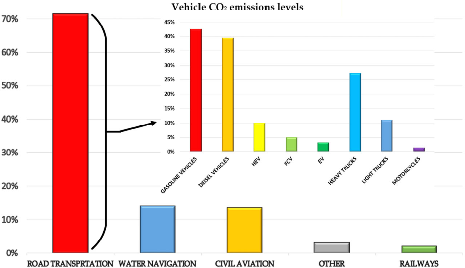
In 2025, the global electric vehicle market recorded a 20% increase, reaching a total of 20.7 million sales [1]. This is largely driven by efforts to combat climate change, as road transport is one of the largest contributors to CO2 emissions. In this context, achieving climate neutrality by 2050 would be impossible for the EU without the electrification of transport. The EU aims to reduce CO2 emissions by 90% by the end of 2035 [2]. The use of renewable energy sources and the electrification of road transportation can reduce greenhouse gas emissions by up to 40%, as illustrated in Figure 1 [3].
The most important component of an electric vehicle is the battery, which also introduces the main limitations: driving range and fast-charging capability. Fast charging involves the use of high currents specific to the charging process, which often leads to significant temperature increases. This factor affects battery lifespan by accelerating the degradation of chemical processes inside the battery, thereby reducing its range, capacity, and durability [4]. A battery pack consists of multiple cells connected in series and in parallel, however, it is impossible for each cell to have identical characteristics. These differences arise from manufacturing tolerances, non-uniform aging, temperature variations, differences in internal resistance, and extreme operating conditions. Each cell has specific characteristics that must be monitored and controlled to increase the lifetime of the cells. In addition, certain limits must be imposed to maximize battery life, such as temperature limits, charging and discharging current limits, discharge current cut-off thresholds, and maximum and minimum cell voltage limits [5].
In a battery pack, the most important component is the Battery Management System (BMS) [6]. The BMS is a system composed of both hardware and software components, and its role is to control the batteries and enhance their performance. Among the functions of the BMS, two of the most important are the estimation of the state of charge (SOC) and the state of health (SOH). Other functions of a BMS include monitoring cell temperatures, performing thermal management, cell balancing, and monitoring the current of the battery pack and its modules [5].
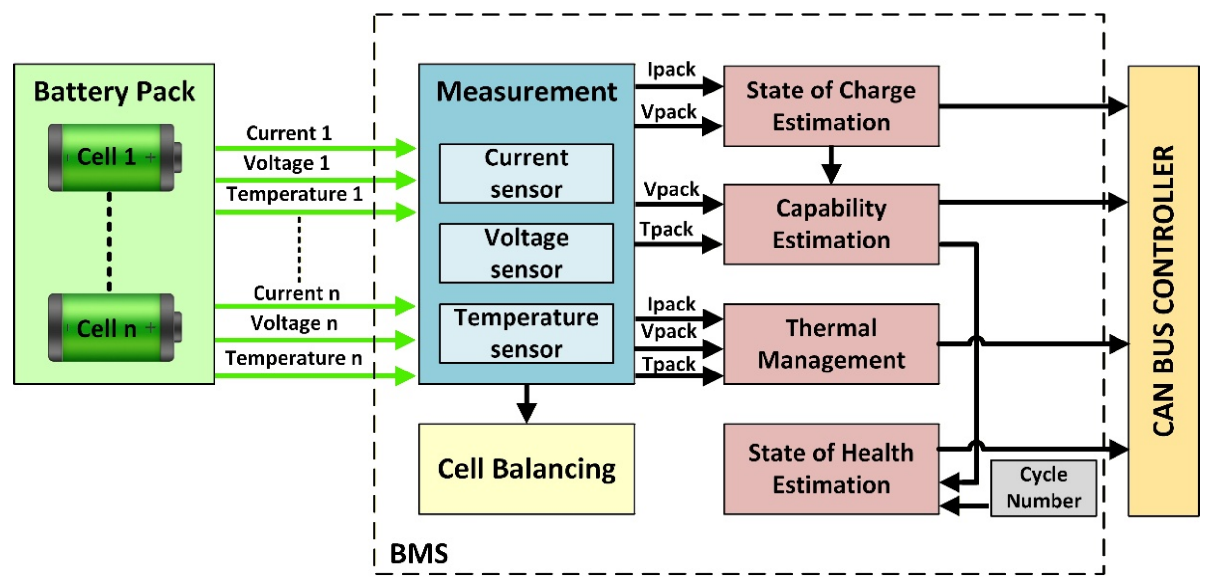
The BMS software (Microsoft Visio Professional 2021) processes data received from sensors in real time and controls the hardware operations to be performed. The block diagram of a BMS is presented in Figure 2 [3].
Cell balancing involves maintaining the voltage of each cell as equal as possible, thereby maximizing the overall performance of the battery pack [3]. When cells are not balanced, some may become overcharged while others remain undercharged. Cells that are charged beyond their allowable limits are the first to experience accelerated aging, capacity degradation, and even the potential onset of thermal runaway. Undercharged cells reduce the total energy capacity of the entire battery pack, leading to decreased overall performance [6].
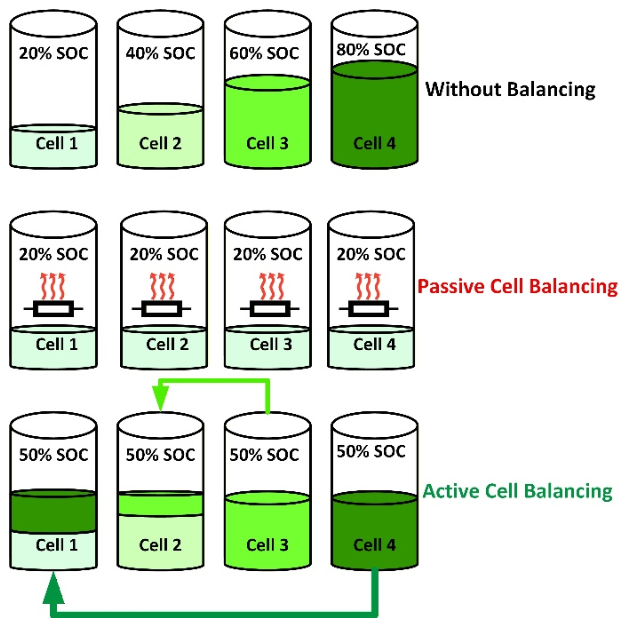
Technical literature identifies two main cell balancing methods: passive balancing and active balancing. The difference between these two methods is illustrated visually in Figure 3.
In the case of passive balancing, the excess energy of a cell with a higher state of charge is dissipated as heat through a resistor. This method is simple and low-cost, but it leads to energy losses and increased temperature, a phenomenon that can negatively affect battery lifespan.
In contrast, active balancing involves transferring energy from cells with a higher state of charge to those with a lower state of charge. This method enables more efficient energy utilization and improves overall battery pack performance; however, it requires more complex circuitry and is therefore associated with higher cost and reduced reliability [7].
Among the numerous active balancing strategies, this paper focuses on active cell balancing using bidirectional flyback converters. In this topology, a transformer is used as an energy storage element and then as an energy transfer medium [8]. To implement this balancing strategy, the DC2100B module was used, which incorporates the LTC3300-1 circuit responsible for controlling the MOSFET switches on both the primary and secondary sides.
Due to the availability of large datasets for various lithium-ion cells, the integration of artificial intelligence into the cell balancing process improves performance and extends the battery remaining useful life (RUL) [9]. This paper aims to present a predictive cell balancing solution for NCR18650B lithium-ion cells, using a model trained on the dataset provided in reference [10], applied to an active balancing strategy based on flyback converters.
Recent advances in battery management systems have explored both enhanced sensing techniques and data-driven control strategies. High-resolution monitoring approaches, such as electrochemical impedance spectroscopy (EIS), enable accurate characterization of lithium-ion battery behavior and internal state estimation [11]. In parallel, machine learning-based active balancing methods, including reinforcement learning and neural network-based controllers, have demonstrated improved efficiency in charge redistribution and state-of-charge equalization [12].
However, these approaches typically focus either on advanced measurement capabilities or on complex control architectures that may be difficult to deploy in real-time embedded systems. In contrast, the present work proposes a lightweight predictive balancing strategy based on a gated recurrent unit (GRU) model, trained directly on experimentally acquired voltage, current, and temperature data and validated within a real-time balancing framework. The proposed method emphasizes practical implementation, reduced computational complexity, and direct integration into a hardware-level battery management system.
This paper is organized as follows: Section 1 introduces the context of battery management systems and the motivation for predictive cell balancing. The section continues with a review of the state of the art in active cell balancing for lithium-ion battery systems, with particular emphasis on inductive balancing topologies, flyback-based architectures, and commonly used control strategies. Section 2 describes the materials and methods, including the hardware platform, the experimental dataset, and the formulation of the predictive voltage estimation problem, as well as the proposed GRU-based model. Section 3 presents the experimental results obtained on a multi-cell battery pack and provides a comparison between the predictive and conventional reactive balancing strategies. Finally, Section 4 discusses the main findings and outlines directions for future work.

1.2. State of the Art

1.2.1. Active Cell Balancing Topologies

The basic principle of active balancing consists of using energy storage components such as capacitors, inductors, or transformers to store energy extracted from cells with a high SOC and transfer it to cells with a lower SOC. Active balancing offers the advantage of utilizing the battery energy more efficiently; however, it requires more complex circuit configurations and advanced control algorithms.
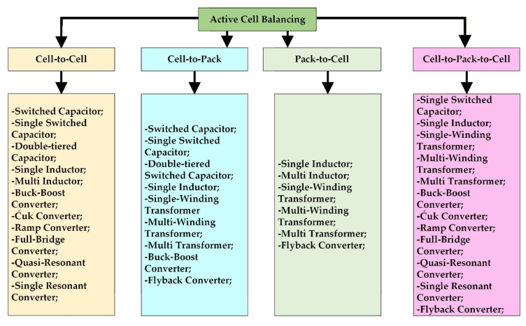
Active balancing relies on the use of specific components such as relays, DC–DC converters, and current sensors. Depending on the energy transfer mechanism, this method can be classified into five main subcategories: Cell Bypass, Cell-to-Cell, Cell-to-Pack, Pack-to-Cell, and Cell-to-Pack-to-Cell [13]. The main types of active balancing are presented in Figure 4.
Active cell balancing using capacitor-based energy transfer circuits is based on a relatively simple principle: excess energy is temporarily stored in capacitors and subsequently transferred to cells with a lower state of charge. When a capacitor that has stored energy in the form of an electric field is connected to a lower potential, it releases the stored energy. The capacitors are activated based on continuous monitoring of the state of charge and voltage of each cell, enabling energy transfer to where it is needed [14].
In capacitor-based balancing circuits, one or more capacitors are connected in parallel with the cells. The voltage difference ΔV between the cell and the capacitor drives the energy transfer. The time constant τ is essential for determining the charging and discharging speed of a capacitor. Based on the formula presented in Equation (1), the optimal capacitor value can be easily determined [14].
τ = R C
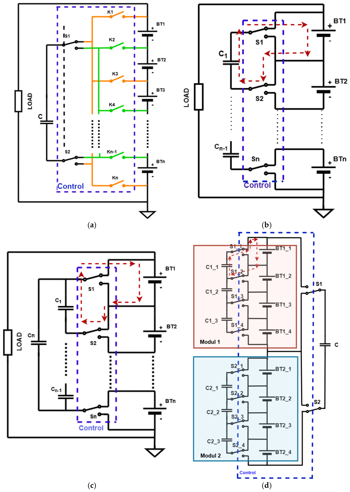
The Single Switched Capacitor topology, illustrated in Figure 5a, is based on a simple control algorithm: the system identifies the cells with the highest and lowest SOC and selectively activates the corresponding switches to enable direct energy transfer between them. This direct energy exchange simplifies the balancing process, making it faster and more efficient compared to other topologies that rely on intermediate transfer stages [15]. The energy transfer within the capacitor can be described as follows: it is assumed that E1 is the cell with higher capacity, while E2 is the cell with lower capacity. Initially, switches K1 and K2 are closed, and switches S1 and S2 are set to the upper position. At this stage, cell E1 transfers charge to the capacitor, which becomes charged with positive charge on the upper plate and negative charge on the lower plate. The charging rate is given by Equation (2) [7]:
Q ˙ = U I = C U d U d t
After this phase, switches K2 and K3 are closed, while S1 and S2 are moved to the lower position, allowing the capacitor to transfer the stored energy to cell E2, thereby completing the balancing process [7].
The Switched Capacitor topology is illustrated in Figure 5b. This approach does not rely on knowledge of the cells’ state of charge (SOC). The topology exhibits high efficiency and supports operation during both charging and discharging conditions. However, it has certain limitations, such as higher cost and longer balancing times. The extended equalization time is mainly due to two factors. First, as the balancing process approaches completion, the voltage difference between two adjacent cells becomes very small. This reduced voltage difference makes it difficult to charge the capacitors and to transfer energy efficiently. Second, energy is transferred only between adjacent cells in each balancing cycle; therefore, multiple cycles are required when energy must be transferred between cells that are farther apart within the battery pack [14].
The Double-Tiered Switched Capacitor topology represents an advanced extension of the conventional Switched Capacitor technique, designed to improve the performance of the cell balancing process. This configuration introduces two capacitor tiers and requires a total of n capacitors and 2n switches to actively balance n cells, as illustrated in Figure 5c. The addition of an extra capacitor tier provides multiple parallel paths for charge transfer, drastically reducing the balancing time by nearly 75% compared to the basic SC method. This improvement in efficiency is particularly important in applications where rapid balancing is essential [14].
Figure 5d presents the Modular Switched Capacitor topology, in which multiple switches are arranged within a battery module. In addition to charge transfer between cells, balancing can also be performed between modules, thereby reducing internal non-uniformities within battery packs [7].
Active balancing can also be implemented using inductor-based circuits. A magnetic field is generated around an inductor when an electric current flows through it. The amount of energy stored in the inductor is directly related to the intensity of the generated magnetic field. When the current changes, the magnetic field intensity changes accordingly. As the current increases, the magnetic field strengthens, and as the current decreases, the magnetic field weakens. Once the current no longer flows through the inductor, the energy stored during conduction is released. The collapsing magnetic field induces a voltage across the inductor, causing current to flow in the opposite direction within the circuit, thereby enabling energy transfer. Inductors are used in active balancing systems to store and transfer energy between battery cells [14].
This method has the advantage that energy from a cell with a higher state of charge can be transferred, using inductors, to a cell with an equal or even lower state of charge, which is not possible with balancing circuits that use capacitors.
The cost of this type of balancing circuit is high, and energy losses occur due to magnetic effects. External capacitors are required as high-frequency filters [7].
The energy stored in an inductor is proportional to the square of the current flowing through it and to the inductance of the inductor, as expressed in Equation (3):
E = 1 2 L I 2
To determine the appropriate size of the inductors, it is essential to consider their charging and discharging principles. The charging and discharging behavior of an inductor is governed by the circuit time constant, τ [15]. The time constant τ for an RL circuit is defined by Equation (4), where L represents the inductance and R represents the internal resistance of the cell.
τ = L R
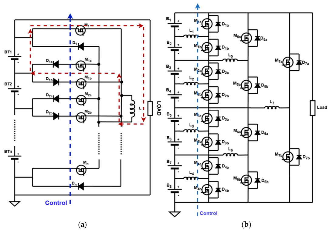
The Single Switched Inductor method presented in Figure 6a enables direct energy transfer between cells by using an inductor to move energy from the cell with the highest state of charge to the cell with the lowest state of charge, thereby achieving direct cell balancing [7].
This technique allows energy to be transferred directly through the inductor from the cell with the highest state of charge in the battery pack to the cell with the lowest state of charge, characterizing this circuit as a cell-to-cell balancing approach. For illustration, let BT1 be the cell with the highest state of charge and BT2 be the cell with the lowest state of charge. Initially, switches M1 and M1a are turned on to charge the inductor. Subsequently, M1 is turned off and M2b is turned on to discharge the inductor and transfer the energy to BT2 [14].
The energy transfer rate is described by Equation (5), where L represents the inductance and U represents the battery terminal voltage [7].
Q ˙ = U I = I L d I d t
The multi-level inductor topology presented in Figure 6b provides a faster balancing time, as it creates additional pathways between intermediate cells. Moreover, this method requires fewer switching devices, leading to higher efficiency and reduced losses. However, a significant drawback is that the number of required inductors increases as more cells are connected in series [15].
Another important category of active balancing methods is based on DC–DC converter topologies, which can be classified into non-isolated and isolated architectures [16].
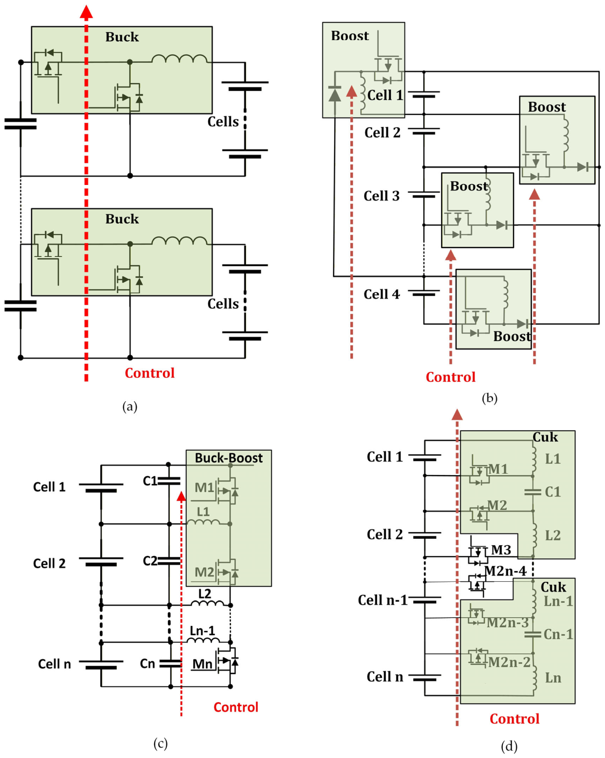
Non-isolated converter-based balancing methods include buck, boost, buck–boost, and Cuk converter topologies, as shown in Figure 7a–d. Unlike non-isolated designs, isolated DC–DC converters use a transformer to provide galvanic separation between input and output, with common examples including flyback, forward, dual active bridge (DAB), dual half-bridge (DHB), resonant, and push–pull topologies [16]. In this work, particular attention is given to the bidirectional flyback converter, which is investigated as a practical solution for energy transfer in active cell balancing applications.
DC-DC balancing provides high balancing accuracy with acceptable balancing efficiency; however, it is associated with increased cost. When a transformer is employed, the primary and secondary windings are galvanically isolated, which enhances balancing performance. Additionally, energy transfer circuits are implemented through secondary windings, enabling energy exchange between battery modules [7].
In balancing circuits using a Buck converter, energy is transferred from a higher-voltage cell to a lower-voltage cell or a common energy storage element by stepping down the voltage. The switch is controlled by a PWM signal, and the inductor temporarily stores energy during the switching process, enabling controlled energy redistribution. Similarly, balancing circuits using a Boost converter, energy is extracted from a lower-voltage cell and boosted to a higher voltage level before being transferred to another cell or to the battery stack. The inductor stores energy when the switch is on and releases it at a higher voltage when the switch is off, allowing energy transfer from weaker cells to stronger ones.
For balancing circuits that use buck–boost converters, a PWM generator with an adjustable duty cycle controls the switching devices, similarly to a conventional buck–boost converter. Inductor L acts as the energy storage element for the balancing process [7,14].
In the case of the Cuk converter, energy is transferred bidirectionally. Each cell is connected to two inductors connected in parallel. Energy is continuously transferred between cells through the capacitors and inductors when the MOSFET transistors are conducting. A major drawback of this method is that energy is transferred only between cells [7,14].

1.2.2. Control Strategies for Active Balancing

This section reviews the main control strategies for active cell balancing, namely voltage-based, SOC-based, and model-based approaches.
In voltage based balancing strategy, the terminal voltage is measured by the BMS and used to determine which cells should be charged and which should be discharged. The decision is typically based either on the average cell voltage or on a predefined threshold value. The sampling frequency can be adjusted, and voltage is easy to measure accurately. However, a drawback of this method is that significant voltage fluctuations may occur due to operating conditions, which can prevent the cells from being properly balanced [7]. The DC2100B-C module from Analog Devices is a representative example of voltage-based cell balancing. In this module, the voltage of all cells is monitored through a graphical interface, and the user determines which cells should be discharged and which should be charged.
The balancing strategy uses the SOC parameter to determine which cells should be charged or discharged. State of charge is widely used as an indicator of the remaining battery capacity, although it cannot be measured directly and must be estimated using methods such as coulomb counting or model-based techniques. Coulomb counting integrates the charge and discharge current over time and is simple to implement, but its accuracy deteriorates due to sensor errors and the lack of inherent self-correction. Model-based approaches, which include physics-based and data-driven methods, estimate SOC using battery models combined with filtering algorithms. Equivalent circuit models are often preferred for real-time applications because they capture cell dynamics with relatively few parameters, whereas electrochemical models offer higher fidelity at the expense of complex parameterization. Among filtering techniques, Kalman-based methods are commonly employed due to their good balance between accuracy and computational cost [7].
Model-based control approaches use mathematical battery models to predict system behavior and optimize energy redistribution among cells. These methods aim to achieve efficient balancing while satisfying operational constraints and improving overall system performance.
Model Predictive Control (MPC) is an advanced control strategy widely applied in engineering, economics, and robotics. It relies on a mathematical model of the system to predict future behavior and determine optimal control actions over a predefined prediction horizon [17].
MPC formulates an optimization problem that minimizes a cost function, such as tracking error or operational cost, while satisfying system constraints. At each sampling instant, the controller solves the optimization using the current system state, applies the first control input, updates the state, and repeats the process, resulting in a receding-horizon feedback control scheme [17].
Fuzzy control strategies, derived from fuzzy logic and artificial intelligence techniques, are considered advanced control methods for systems with uncertain or difficult-to-model dynamics. They enable control decisions through rule-based inference rather than explicit mathematical formulations, although their stability and robustness are typically validated through Hardware-in-the-Loop (HIL) testing rather than strict analytical proofs. In battery balancing applications, multi-input fuzzy controllers can incorporate variables such as voltage deviation, average voltage, temperature, SOC, and SOC-related metrics, allowing coordinated control actions to achieve effective cell equalization [7].
Neural network-based control strategies are generally more complex than conventional methods because they require extensive training data and model development. In these approaches, the balancing system is typically formulated as a nonlinear control problem, and multilayer neural networks are employed to capture the system’s dynamic behavior. Neural network controllers can also be integrated with other control algorithms to further enhance overall balancing performance.

2. Materials and Methods

2.1. Hardware Platform for Active Balancing Control: DC2100B-C

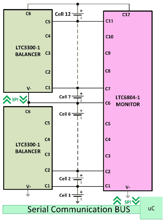
The DC2100B-C evaluation board developed by Linear Technology provides an efficient platform for active balancing of series-connected lithium-ion cells. The system is built around the LTC3300-1 active balancing controller, a PIC18F47J53 microcontroller, and the LTC6804-1 device used for precise cell voltage measurement, forming a complete battery management solution [18].
The LTC3300-1 integrated circuit, produced by Linear Technology, specializes for bidirectional active cell balancing, using flyback converters to transfer energy between cells. The circuit can transfer energy in both directions, selectively charging or discharging a cell. One LTC3300-1 can manage six lithium-ion cells simultaneously. Multiple LTC3300-1 circuits can be connected in a daisy-chain configuration, allowing them to operate in large battery packs without requiring additional isolation components.
In the battery management system shown in Figure 8, the LTC6804-1 integrated circuit accurately measures the individual cell voltages and provides information about the state of the battery stack to the PIC18F47J53 microcontroller [4]. The first step in the BMS operating flow is the measurement of each cell voltage in the stack and the transmission of these values to the microcontroller via the SPI interface. The microcontroller calculates the voltage differences between cells and determines which cells must be discharged and which must be charged, in what sequence, and at what current level.
The DC2100B-C is supplied with a graphical user interface that enables configuration and real-time monitoring of the balancing process. Users can select balancing actions for individual cells or perform timer-based balancing by specifying a predefined duration.

2.1.1. The Configuration of the Analyzed Cell Balancing Circuit

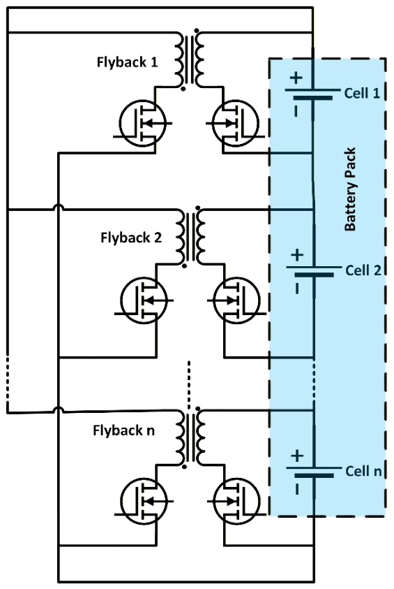
Figure 9 illustrates the architecture of the proposed modular cell-balancing system built around synchronous flyback converter units. The battery pack is composed of multiple series-connected cells that require voltage equalization. Each cell is paired with a symmetrically designed bidirectional flyback converter, where a flyback converter is selected because it offers galvanic isolation, a straightforward topology, and broad applicability, which helps lower both the cost and structural complexity of the balancing solution. All synchronous flyback converter modules are arranged as follows: the secondary windings are connected in parallel across the entire battery pack, while the primary windings interface directly with the individual cells. The switching devices on the secondary side must be rated for full pack voltage, whereas components with lower voltage ratings are sufficient on the primary side. Because every cell is associated with its own bidirectional flyback converter, the system gains increased flexibility for bidirectional energy transfer and coordinated balancing among cells [8].
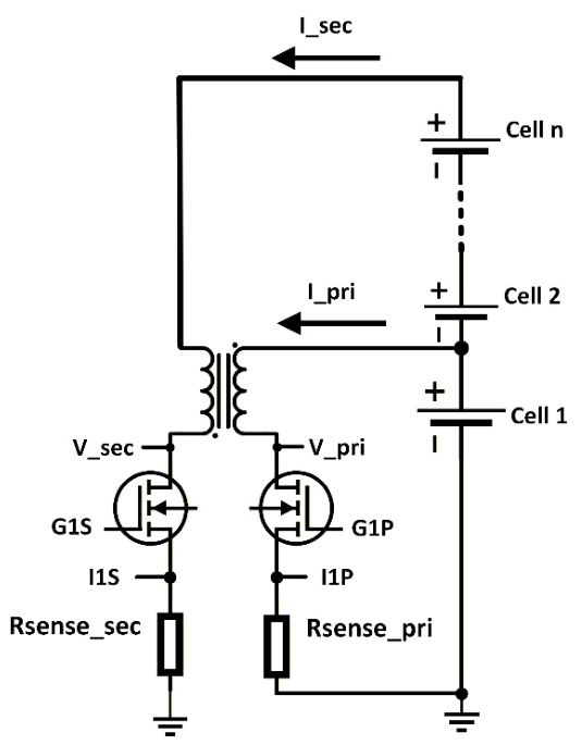
Figure 10 presents the configuration of a single synchronous flyback converter connected in parallel with an individual battery cell. An identical flyback module is associated with each cell in the pack. As shown in Figure 10, the external NMOS transistor placed in series with the transformer primary winding is driven by the G1P gate signal. In a similar manner, the NMOS transistor connected in series with the secondary winding—whose corresponding primary is paralleled with Cell 1—is controlled by the G1S gate signal [19].

2.1.2. Operation Principle of Synchronous Flyback Converter

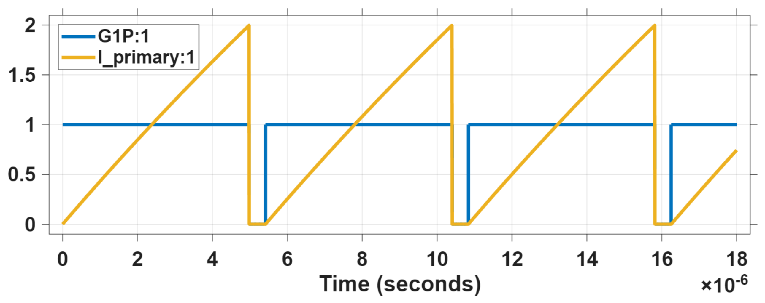
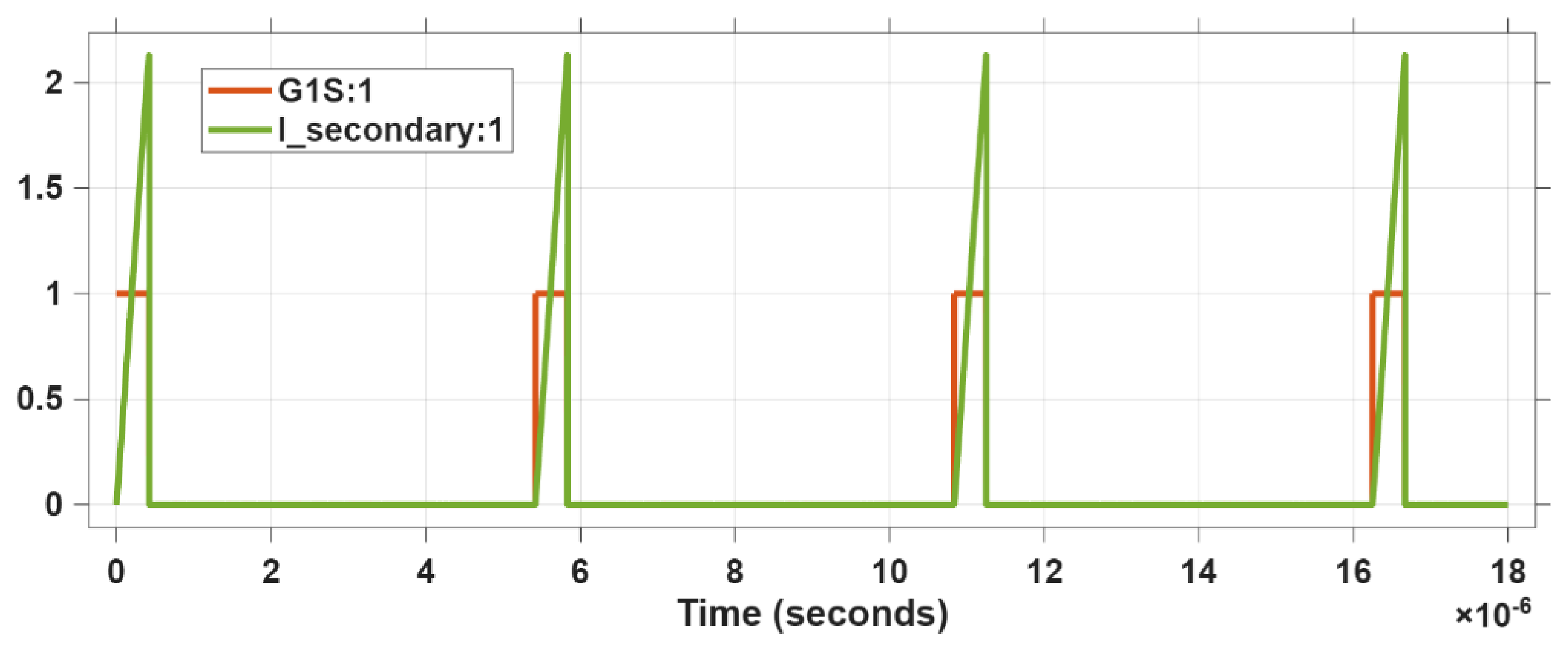
Assume that in the circuit shown in Figure 9, Cell 1 has a higher voltage than the other cells in the battery pack. To discharge this cell and bring its voltage closer to the others, the primary-side switch is turned on, causing the current in the transformer primary winding to ramp up until it reaches the programmed peak current (Ipp) detected at pin I1P [8,20,21].
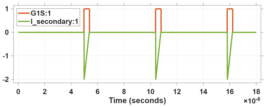
Once the primary current reaches the peak value, the primary-side switch is turned off, and the energy stored in the transformer is transferred to the cells connected in series on the secondary side. During the energy transfer interval, the secondary-side switch is ON to minimize power losses until the secondary current drops to zero, as detected at pin I1S. The switching cycle restarts once the secondary current reaches zero.
The peak current I p p is given by Equation (6), where V s e n s e _ r e f   is the internal reference voltage of the current-sense circuit.
I p p = V sense _ ref R sense _ pri
The cell discharge current on primary side, I dis   and the charging current of the secondary-side cells, I sec , are determined by Equations (7) and (8), where N is the number of cells on the secondary side, 1:T is the transformer turns ratio from primary to secondary, and η d i s is the energy transfer efficiency from the discharged primary-side cell to the secondary-side cell pack.
I dis = I pp 2 ( N N + T )
I sec = I pp 2 ( 1 N + T ) η d i s
Considering a battery pack with N = 12 cells, T = 1, and V sense _ ref = 50 mV, the current in the primary and the current through the secondary have the waveform shown in Figure 11, corresponding to the discharge of cell 1.
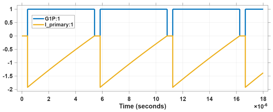
Assume that in the circuit shown in Figure 9, Cell 1 has a lower voltage than the other cells in the battery pack. To charge this cell and bring its voltage closer to the others, the secondary-side switch corresponding to Cell 1 is turned on, causing current to flow from the secondary-side cells through the transformer until it reaches the programmed peak current detected at pin I1S [20,21].
Once the secondary current reaches the peak value, Ips, the secondary-side switch is turned off, and the energy stored in the transformer is transferred to the primary side, thus charging the selected cell. During the energy transfer interval, the primary-side switch is ON to minimize power losses until the primary current drops to zero, as detected at pin I1P. The switching cycle restarts once the primary current reaches zero.
The peak current is given by Equation (9).
I p s = V sense _ ref R sense _ sec
The cell charges current, I chg   and the discharge current of the secondary-side cells, are determined by Equations (10) and (11), where η c h g represents the efficiency of energy transfer from the secondary-side cell stack to the primary-side cell [20].
I c h g = I ps 2 ( N T N + T ) η c h g
I sec = I ps 2 ( T N + T )
Considering a battery pack with N = 12 cells, T = 1, and V sense _ ref = 50 mV, the primary and secondary currents have the waveform shown in Figure 12, corresponding to the charging of cell 1.
In this cell balancing circuit, the balancing current is not directly measurable. Instead, it is often inferred indirectly from the variation of the cell’s state of charge, which can be estimated from voltage measurements and electrochemical models. This approach is justified by the fact that active balancing strategies aim to equalize the SoC among cells, while the transferred energy is implicitly governed by this state variable rather than explicitly controlled current measurements.
The estimation of the balancing current is derived from the fundamental definition of SoC, which is based on Coulomb counting. By rearranging this relationship, the average balancing current over a given time interval can be expressed with Equation (12), where Q   is the nominal capacity of the cell, Δ S o C   represents the change in state of charge, and Δ t is the corresponding time interval.
I b a l Q Δ S o C Δ t
In the absence of direct current measurement, the SoC can be estimated from the cell terminal voltage using the open-circuit voltage (OCV) relationship. In practice, this relationship is implemented as a lookup table or an empirically derived function, given by Equation (13). The inverse mapping is then used to estimate the state of charge from measured voltage values. This method is well established in literature and is commonly used to calibrate and support current-based estimation techniques. However, its accuracy depends strongly on the battery chemistry and the flatness of the OCV curve.
V O C = f ( S o C )

2.2. Dataset and Problem Formulation

2.2.1. Battery Dataset Description

The predictive model proposed in this work was trained using experimental datasets obtained from NCR18650B lithium-ion cells from [10]. The datasets were collected under controlled laboratory conditions and include multiple dynamic current profiles and temperature levels to capture the voltage response of the cells under a wide range of operating conditions relevant to electric vehicle battery packs.
The dataset contains measurements acquired from commercial Panasonic NCR18650B cylindrical cells with a nominal capacity of 3.4 Ah and nominal voltage of 3.6 V. Each dataset includes time-series measurements of cell voltage, applied current, and elapsed time. The sampling interval was constant within each experiment and equal to 1 s. All measurements were recorded using calibrated laboratory equipment and verified to remove corrupted or incomplete samples. The dataset was constructed using several experimental tests, which are described in the following paragraphs [10].
To ensure robustness of the predictive model, several standard drive-cycle-based current profiles were considered. These profiles reproduce realistic operating conditions such as acceleration, regenerative braking, and steady-state driving. The dataset also includes measurements at different ambient temperatures to capture temperature-dependent battery dynamics. Experiments were conducted at −5 °C, 5 °C, 25 °C, and 45 °C using a temperature-controlled chamber [10].
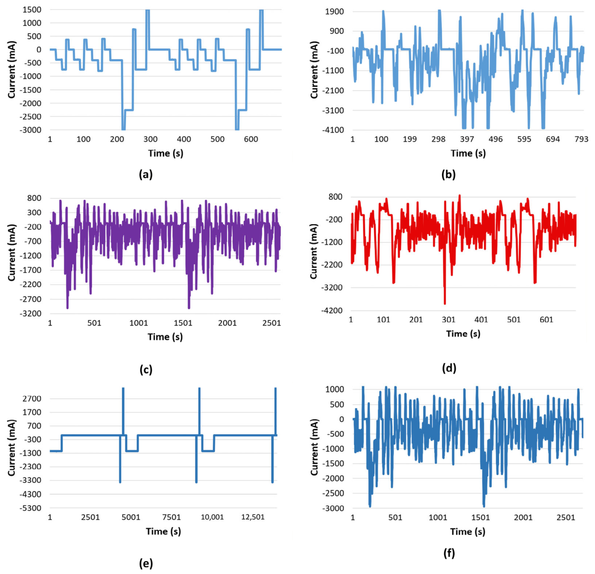
Dynamic Stress Test (DST) introduces rapid and frequent current variations, allowing the model to learn short-term voltage dynamics under highly transient operating conditions. Figure 13a presents the current–time profile of the DST scenario from the Lithium-ion Battery Dynamic Stress Test Dataset, highlighting the rapid and frequent current fluctuations used to excite short-term voltage dynamics and support predictive balancing model training. For all temperature settings in the Lithium-ion Battery Dynamic Stress Test Dataset, the DST scenario preserved the same sequence of current levels, while the number of time samples differed.
Federal Urban Driving Schedule (FUDS) represents stop-and-go urban driving with moderate accelerations, providing data that reflects typical city operation of electric vehicles. Figure 13b shows the current profile of the FUDS scenario, illustrating the characteristic stop-and-go current variations of urban driving. The same current sequence was applied at all tested temperatures, with differences only in the number of recorded time samples.
Urban Dynamometer Driving Schedule (UDDS) simulates standardized urban driving with repeated acceleration and deceleration phases, capturing voltage behavior during low-speed vehicle operation. Figure 13c presents the current–time profile of the UDDS scenario from the Lithium-ion Battery Dynamic Stress Test Dataset, highlighting the repeated acceleration–deceleration current pattern characteristic of standardized low-speed urban driving. For all temperature settings in the Lithium-ion Battery Dynamic Stress Test Dataset, the UDDS scenario preserved the same sequence of current levels, while the number of recorded samples differed due to variations in sampling duration.
US06 Driving Cycle (US06) includes aggressive accelerations and higher power demand, enabling the model to learn voltage response under high-load and dynamic driving conditions. Figure 13d presents the current–time profile of the US06 scenario from the Lithium-ion Battery Dynamic Stress Test Dataset, highlighting the aggressive acceleration patterns and high-power demand characteristic of dynamic, high-load driving conditions and their relevance for predictive balancing model training. For all temperature settings in the Lithium-ion Battery Dynamic Stress Test Dataset, the US06 scenario preserved the same sequence of current levels, while the number of recorded samples differed due to variations in sampling duration [10].
Worldwide Harmonized Light Vehicles Test Procedure (WLTP/WLTS) combines urban and highway driving phases and represents modern real-world vehicle operation, offering realistic load variations across a wide operating range. Figure 13e shows the current–time profile of the WLTP/WLTS scenario from the Lithium-ion Battery Dynamic Stress Test Dataset, illustrating the combined urban–highway load pattern of realistic driving conditions. The same current sequence was applied at all tested temperatures, with differences only in the number of recorded time samples.
Hybrid Pulse Power Characterization (HPPC) tests consist of controlled charge and discharge pulses at different states of charge, providing information about transient voltage response and internal resistance behavior. Figure 13f presents the current–time profile of the HPPC scenario highlighting the controlled charge and discharge pulse sequence applied. For all temperature settings in the Lithium-ion Battery Dynamic Stress Test Dataset, the HPPC scenario preserved the same sequence of current levels, while the number of recorded time samples differed due to variations in sampling duration.
Constant-Current Charge and Discharge Tests (0.5 C, 1 C, 1.5 C) capture quasi-steady-state voltage behavior at different current levels and establish baseline voltage–current relationships. The dataset was partitioned into training, validation, and test sets in an approximate proportion of 70%, 15%, and 15%, respectively.
For each temperature level, multiple current profiles were applied, resulting in a total dataset containing 722,300 samples. Table 1 summarizes the dataset composition.

2.2.2. Predictive Voltage Estimation Problem

Cell terminal voltage is one of the primary measurable variables in lithium-ion battery management systems because it reflects instantaneous operating conditions, proximity to safety limits, and internal electrochemical dynamics such as polarization and ohmic drops. Consequently, short-term voltage prediction has been widely investigated as an enabling tool for advanced BMS functions including early warning, diagnostics, and control decision-making under future operating conditions [21].
In applications where control actions depend on future system behavior, multi-step voltage forecasting becomes more relevant than one-step prediction. Several recent studies demonstrate the use of recurrent neural networks, particularly GRU-based models, to predict battery voltage multiple steps ahead using real driving cycle data, highlighting their ability to capture nonlinear temporal dependencies in battery dynamics [22].
In this work, the predictive estimation problem is formulated as a supervised time-series forecasting task. For each cell i, the goal is to estimate future voltages V (k + h) over a short horizon h ∈ [1,H] using a sliding window of past measurements. Using voltage, current, and temperature as input features is common in battery data-driven modeling because terminal voltage strongly depends on load current and temperature-dependent electrochemical kinetics, and these signals are typically available in practical BMS hardware [23].
To construct the supervised dataset, a sliding-window approach is used to transform sequential measurements into input–output training pairs. A window of length N samples is mapped to a prediction target consisting of future voltage values over the horizon H. This formulation is widely used in battery forecasting studies and in general time-series prediction problems to enable supervised learning from sequential sensor data.
Multistep prediction can be implemented using either direct forecasting, where the model outputs all future steps simultaneously, or recursive forecasting, where predictions are iteratively fed back as inputs. In battery voltage prediction literature, multi-forward-step strategies are frequently adopted to improve stability and to avoid error accumulation in recursive approaches, especially under highly dynamic load profiles [22].
From an implementation perspective, predictive models used in BMS must balance accuracy and computational complexity. GRU architectures are often preferred over LSTM in embedded battery applications because they have fewer parameters and lower computational cost while still capturing temporal dependencies effectively, making them suitable for real-time estimation in resource-constrained systems [24].
Model training is typically performed by minimizing prediction error between measured and predicted voltages across the forecasting horizon. Performance is commonly evaluated using metrics such as Mean Absolute Error (MAE), Root Mean Square Error (RMSE), and Mean Absolute Percentage Error (MAPE), which are widely adopted in battery prediction literature to compare forecasting accuracy across datasets and operating conditions.
Short-horizon prediction (1–10 s) is particularly challenging because battery voltage contains both fast transient components and nonlinear behavior under dynamic loads. Therefore, many studies compare data-driven models with equivalent circuit or autoregressive models to quantify improvements in prediction accuracy under realistic driving cycles, emphasizing the need for experimental validation on real battery packs [25].
Predictive active balancing addresses the limitation of reactive strategies by anticipating short-term cell voltage evolution, enabling earlier and more efficient energy redistribution under dynamic operating conditions, reduced voltage spread, improved converter utilization, and increased usable battery capacity.

2.3. Proposed Predictive Voltage Model

2.3.1. Artificial Neural Networks (ANN)

An artificial neural network (ANN) is a computational framework inspired by the functioning of the human brain. Like biological neural systems, the fundamental element of this structure is the neuron. A biological neuron consists of three primary components: dendrites, which receive signals from other neurons, the cell body that processes these signals, and the axon that transmits information to neighboring neurons through synaptic connections. In artificial intelligence models, dendrites correspond to input signals, the axon represents the output, and synapses are modeled as adjustable connection weights [22].
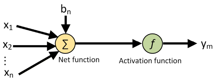
Figure 14 presents the architecture of an artificial neuron. In this representation, X = [ x 1 , x 2 , x 3 , , x n ] , n N denotes the input vector, while W = [ W 1 , W 2 , W 3 , , W n ] , n N represents the vector of connection weights. The net input is computed as the weighted sum of the inputs, to which a bias term b 1 is added. The resulting value is then processed by an activation function f , producing the neuron output y m . Activation functions may be either linear or nonlinear. Linear functions are typically suitable for relatively simple tasks, such as curve fitting, whereas nonlinear activation functions, including the rectified linear unit (ReLU), sigmoid, and hyperbolic tangent, enable neural networks to capture more complex relationships and significantly enhance their modeling capability [22].
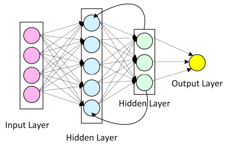
Artificial neural networks (ANNs) are formed by interconnecting multiple artificial neurons into a structured computational system. Typically, an ANN is organized into three types of layers: an input layer, an output layer, and one or more intermediate layers known as hidden layers, which do not interact directly with external data. In conventional feed-forward neural networks, information propagates in a single direction from the input layer to the output layer, without incorporating any form of temporal dependency between successive inputs. However, many real-world problems involve sequential data where current outputs depend on previously observed information. To address this limitation, recurrent neural networks (RNNs) extend the classical ANN architecture by introducing recurrent connections that enable the network to retain information from previous time steps and model temporal dynamics. Figure 15 presents the architecture of a recurrent neural network.

2.3.2. Gated Recurrent Unit (GRU) Networks

The predictive voltage estimator is implemented using a GRU neural network, a type of recurrent neural network designed for sequential data modeling. GRU networks were introduced to address limitations of standard RNNs, particularly the vanishing gradient problem, while maintaining lower computational complexity compared with LSTM architectures. This makes GRU models suitable for embedded battery management systems that require real-time prediction with limited hardware resources.
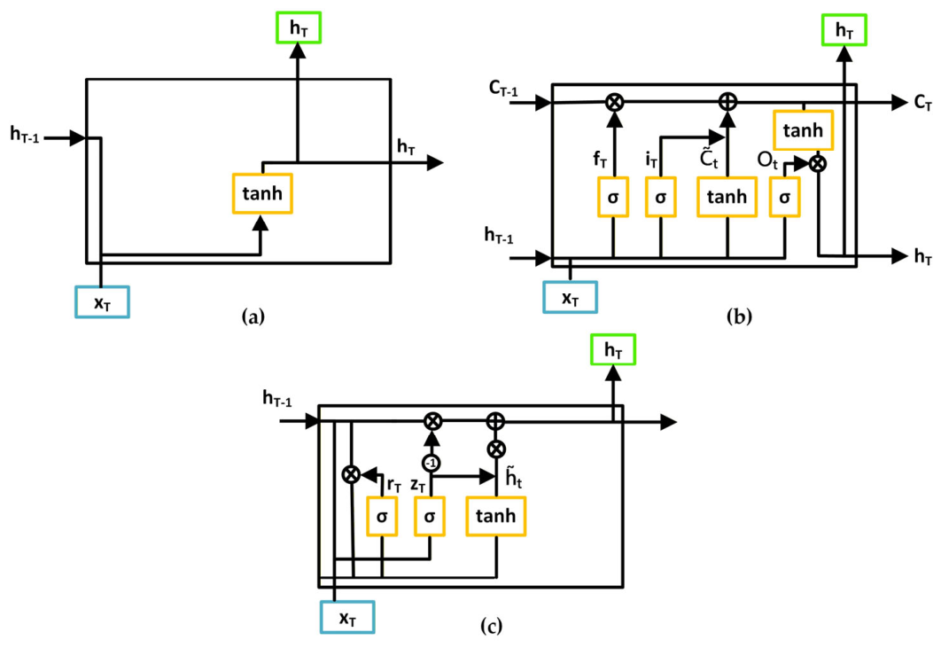
Long Short-Term Memory (LSTM) networks were developed as an extension of the Recurrent Neural Network (RNN) architecture to better capture long-term dependencies in sequential data. Later, Cho et al. introduced the Gated Recurrent Unit (GRU), a simplified recurrent architecture designed to reduce the complexity of LSTM while maintaining the ability to model temporal relationships. The overall structures of RNN, LSTM, and GRU are illustrated in Figure 16. Compared with basic RNN architecture, LSTM includes a more complex internal structure [23].
The fundamental components of an LSTM unit consist of a memory cell state c T and three gating mechanisms: the input gate, forget gate, and output gate. These gates regulate the flow of information within the network and allow the model to preserve or discard information over time. The matrices W and b correspond to the weight parameters and bias terms associated with each gate, while the subscripts f, i, and o denote the forget, input, and output gates, respectively [23].
The cell state ( c T ) can be viewed as a pathway that runs across the LSTM unit and enables information to propagate through successive time steps. This mechanism allows relevant information to be preserved while irrelevant data can be filtered out during the learning process.
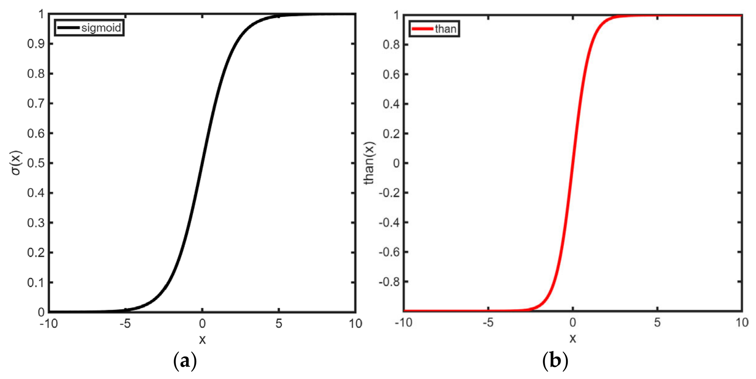
When the hidden state from the previous time step T − 1 ( h T 1 )   together with the current input at time T ( x T ) are fed into the LSTM unit, the forget gate f T   determines which information from the previous cell state should be retained or discarded. The forget gate is computed by Equation (14), where σ is the sigmoid layer, given by Equation (15) and shown in Figure 17a. The sigmoid activation function maps real-valued inputs into the interval (0, 1), providing a smooth and differentiable transformation that is particularly suitable for modeling probabilities and enabling gradient-based optimization during neural network training [23].
f T = σ ( W f [ h T 1 , x T ] + b f )
σ ( x ) = ( 1 + e x ) 1
The LSTM architecture employs an input gate i T together with the input layer C T ~ to regulate the amount of new information stored in the cell state, here t a n h denotes the hyperbolic tangent activation function as shown in Figure 17b. W c represents the weight matrix of the input layer, while b c corresponds to its bias vector [23].
i T = σ ( W i [ h T 1 , x T ] + b i )
C   T ~ =   t a n h ( W c   [ h T 1 , x T   ] + b c )
The previous cell state is then updated to produce the new cell state C T 1 . This update combines the information retained from the past with the cell state C T based on Equation (18). The symbol ∘ denotes the Hadamard product, which performs element-wise multiplication between vectors or matrices of the same dimension [24].
C T = f T C T 1 + i T C T ~
Finally, the output gate o T determines which parts of the cell state will contribute to the hidden state, based on (19) and (20), where h T represents the hidden state at time step T which corresponds to the output O u t T .
o T = σ ( W o [ h T 1 , x T ] + b o )
h T = o T tanh ( C T )
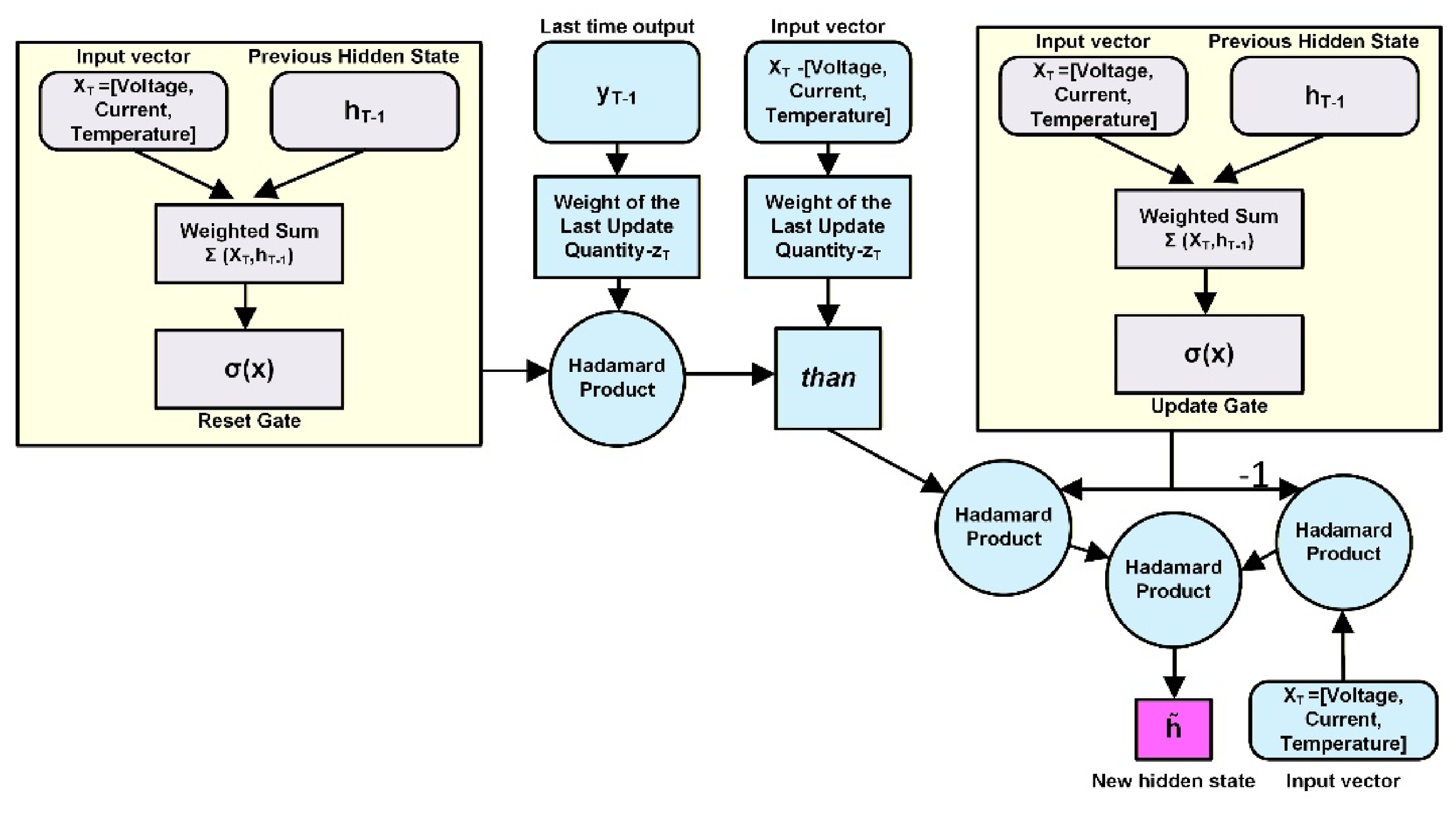
Based on the LSTM architecture, the GRU model simplifies the gating mechanism by combining the forget gate and the input gate into a single update gate z T , while also merging the cell state with the hidden state. This design reduces the model complexity and computational cost. As a result, GRU relies on two gates only: the reset gate r T and the update gate z T defined by Equations (21) and (22), where W T and W z denote the weight matrices of the reset and update gates, respectively, and b r and b z are the corresponding bias vectors [23].
r T = σ ( W r [ h T 1 , x T ] + b r )
z T = σ ( W z [ h T 1 , x T ] + b z )
The new memory state will be obtained by Equation (23), where W h and b h are the weight matrix and bias vector are associated with the new memory cell state [23].
h   T ~ =   t a n h ( W h   [ h T 1 , x T   ] + b h )
The update gate takes values in the interval [ 0 , 1 ] . Values close to 1 allow more information from the new memory cell state to be incorporated, while values close to 0 retain more information from the previous hidden state. Consequently, the final hidden state is computed as:
h T = ( 1 z T ) h T 1 + z T h T ~
Compared to alternative recurrent neural network architectures, the GRU provides an effective compromise between accuracy and computational efficiency. While conventional RNNs struggle to model long-term temporal dependencies, and LSTM networks introduce increased architectural complexity and computational overhead, GRUs achieve comparable performance with a more compact structure. This characteristic makes them well-suited for practical battery management systems, where real-time operation and limited computational resources are critical constraints [25].

2.3.3. Model Architecture

The proposed model was implemented in Python 3.14 using the TensorFlow/Keras framework. The data processing pipeline was developed using NumPy and Pandas, while model evaluation and visualization were performed using scikit-learn and Matplotlib 3.10.8. All simulations and model training procedures were carried out on Windows 11, with an AMD Ryzen 9 4900H processor (3.30 GHz), 24 GB of RAM, and an NVIDIA GPU with 6 GB of memory. The computational setup was sufficient to ensure efficient training and evaluation of the proposed GRU model.
The implemented neural network architecture consists of two stacked GRU layers containing 64 and 32 hidden units. The first recurrent layer processes the input temporal sequence and outputs a sequence of hidden representations, which are further processed by the second GRU layer to extract higher-level temporal features. To improve the generalization capability of the model and reduce overfitting, a dropout regularization layer with a dropout rate of 0.2 is introduced between the two recurrent layers.
At each time step, the input variables are first linearly transformed and then passed through nonlinear activation functions such as the sigmoid and hyperbolic tangent (tanh). These operations allow the network to update its internal hidden states and capture temporal dependencies in the measured signals.
For the implemented model, the input vector at time step t   is defined as
x t = [ V t I t T t ]
where V t , I t , and T t   are the measured battery voltage, current, and temperature, respectively.
The output of the recurrent network is connected to a fully connected dense layer with H neurons, where H denotes the prediction horizon. This layer produces a direct multi-step forecast of the battery voltage over the interval [t + 1, t + H]. The network receives as input a sliding time window containing 60 consecutive measurements of battery voltage, current, and temperature. These sequential measurements allow the model to capture the temporal dependencies present in the battery dynamics. In this study, separate models were trained for different prediction horizons (H = 1, H = 5 and H = 10). For each case, the model outputs a vector of future voltage estimates, while the prediction corresponding to the final time step t + H is used for performance evaluation. The architecture of the proposed GRU-based voltage prediction model is illustrated in Figure 18.
Each model was trained using the mean squared error as the loss function and the Adam optimization algorithm. Training was performed for a maximum of 50 epochs, with early stopping applied based on the validation loss to prevent overfitting. The computation flow within the GRU unit, including gate operations and hidden state update, is shown in Figure 19.

2.3.4. Prediction Performance

The model was evaluated on an independent test set consisting of WLTS driving profiles, which were not used during training or validation.
First, a one-step-ahead prediction framework was performed, where the GRU model predicts the cell voltage at t + 1   using a sequence of past measurements of voltage, current, and temperature.
The GRU-based model was trained for a maximum of 50 epochs using the Adam optimizer, with an initial learning rate of 1 × 10 3 . A learning rate reduction strategy was applied during training, allowing the optimizer to progressively decrease the step size as the validation loss plateaued.
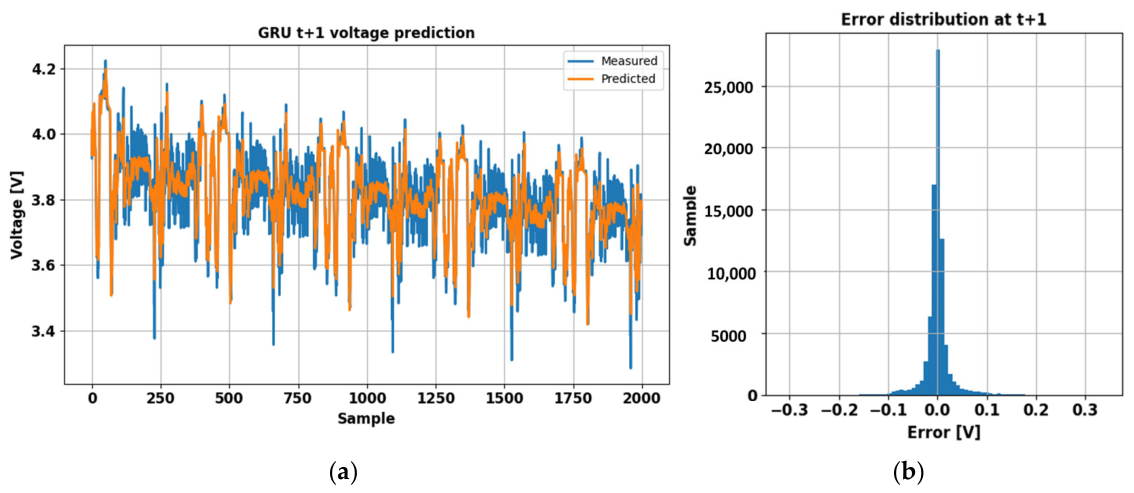
As shown in Figure 20a, the predicted voltage closely follows the measured voltage over the entire test sequence. The model captures both the global trend and the local variations, indicating a strong temporal modeling capability. The prediction error over time is illustrated in Figure 20b. The error remains centered around zero, suggesting the absence of systematic bias.
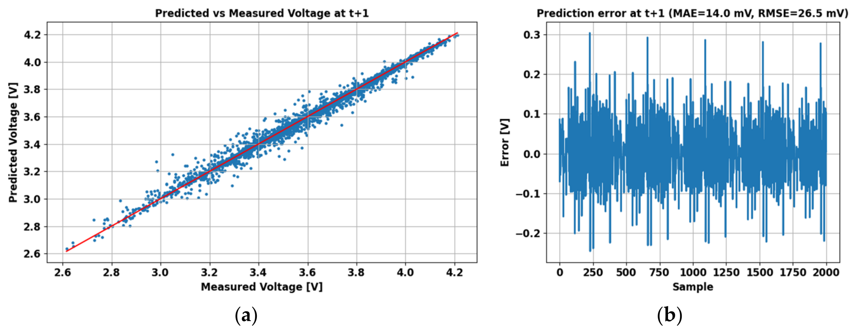
The correlation between measured and predicted voltages is shown in Figure 21a. The data points are tightly clustered around the red line which represent the measured voltage, demonstrating a strong agreement between predicted and actual values and confirming the high predictive accuracy of the model. The prediction error is shown in Figure 21b, with an MAE = 14 mV.
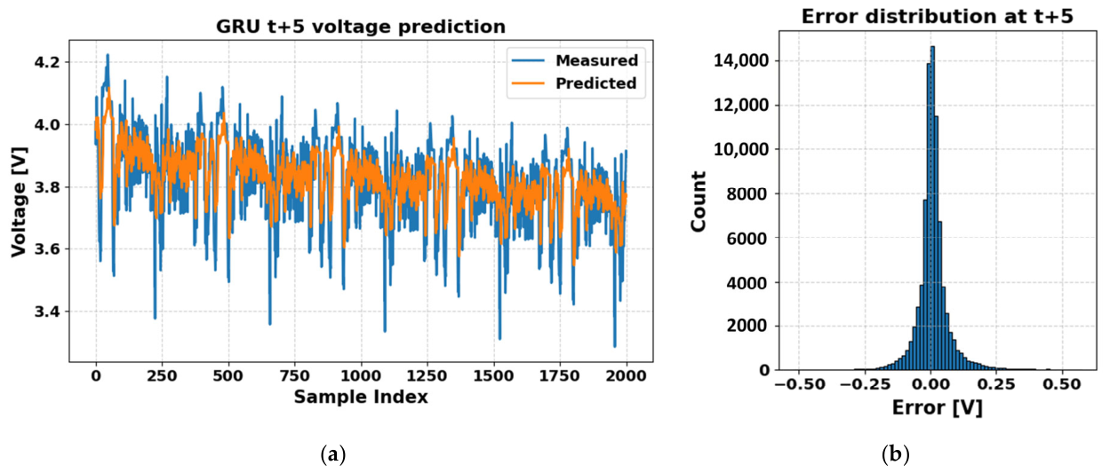
The predictive performance of the model was further evaluated for a longer prediction horizon of five steps ahead (t + 5). As illustrated in Figure 22a, the predicted voltage continues to follow the overall trend of the measured signal at t + 5. However, a slight smoothing effect can be observed, particularly during rapid transients. The corresponding prediction error is shown in Figure 22b. Compared to the t + 1 case, the error magnitude increases, especially during high-dynamic regions, while remaining centered around zero.
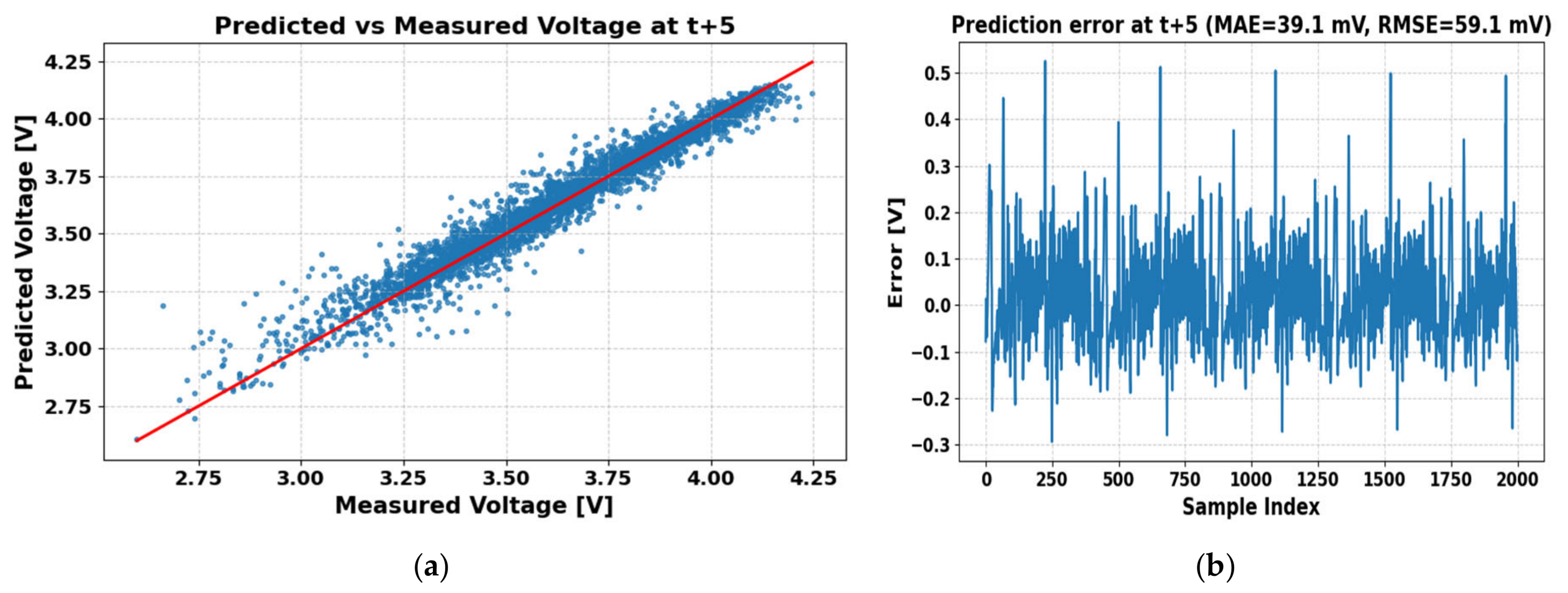
As shown in Figure 23a, the predicted values remain well correlated with the measured voltage (red line), although a slightly larger dispersion around the identity line is noticeable. The prediction error is shown in Figure 23b, with an MAE of 39.1 mV.
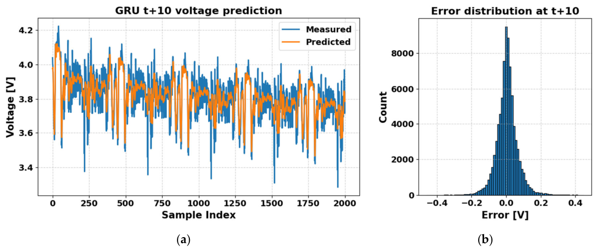
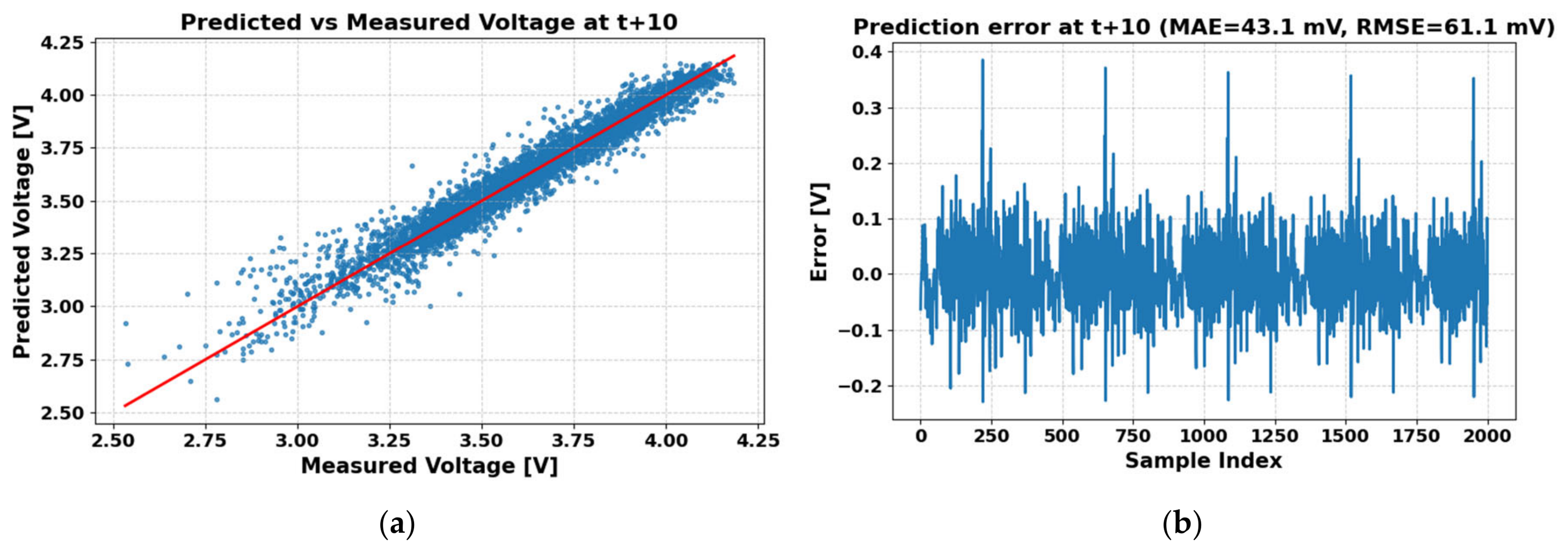
Figure 24 and Figure 25 present the voltage prediction results for the t + 10 case. As expected, the longer prediction horizon leads to a more challenging estimation task. Even so, the predicted signal preserves the general evolution of the measured voltage, while the error remains within an acceptable range for most samples.
In Figure 24a, the predicted voltage reproduces the main behavior of the measured signal over the test interval, although small deviations become more visible during rapid fluctuations. The corresponding error distribution shown in Figure 24b remains centered around zero, indicating the absence of systematic bias. However, in comparison with the t + 1 and t + 5 cases, a clear broadening of the distribution is observed, with heavier tails, reflecting the increased uncertainty associated with the extended prediction horizon.
A quantitative comparison of the prediction accuracy for different horizons is provided in Table 2, where MAE and RMSE are reported for t + 1, t + 5, and t + 10.
The residual prediction errors can be attributed to several factors related to both the physical characteristics of lithium-ion cells and the limitations of data-driven models. Battery voltage exhibits nonlinear and history-dependent behavior influenced by state of charge, temperature, and electrochemical hysteresis, which cannot be fully captured using a finite input window of past measurements.
Moreover, the increase in prediction error with the forecasting horizon is consistent with findings in the literature, where recurrent neural network models show reduced accuracy as the prediction horizon increases due to the accumulation of uncertainty over multiple steps [27].
Additionally, the smoothing effect observed in the predicted signal during rapid transients is a known characteristic of neural networks trained using mean squared error, which tend to favor average trends over sharp variations. This limitation is particularly evident in highly dynamic operating conditions, where data-driven models may fail to fully capture fast system responses [25].
Finally, the use of an estimated current signal introduces an additional source of uncertainty, as the input itself is affected by modeling assumptions. Similar limitations of machine learning-based approaches for battery modeling have been reported in the literature, where the accuracy of predictions strongly depends on input quality and the ability of the model to represent complex electrochemical dynamics [25].

3. Experimental Results

3.1. Experimental Setup

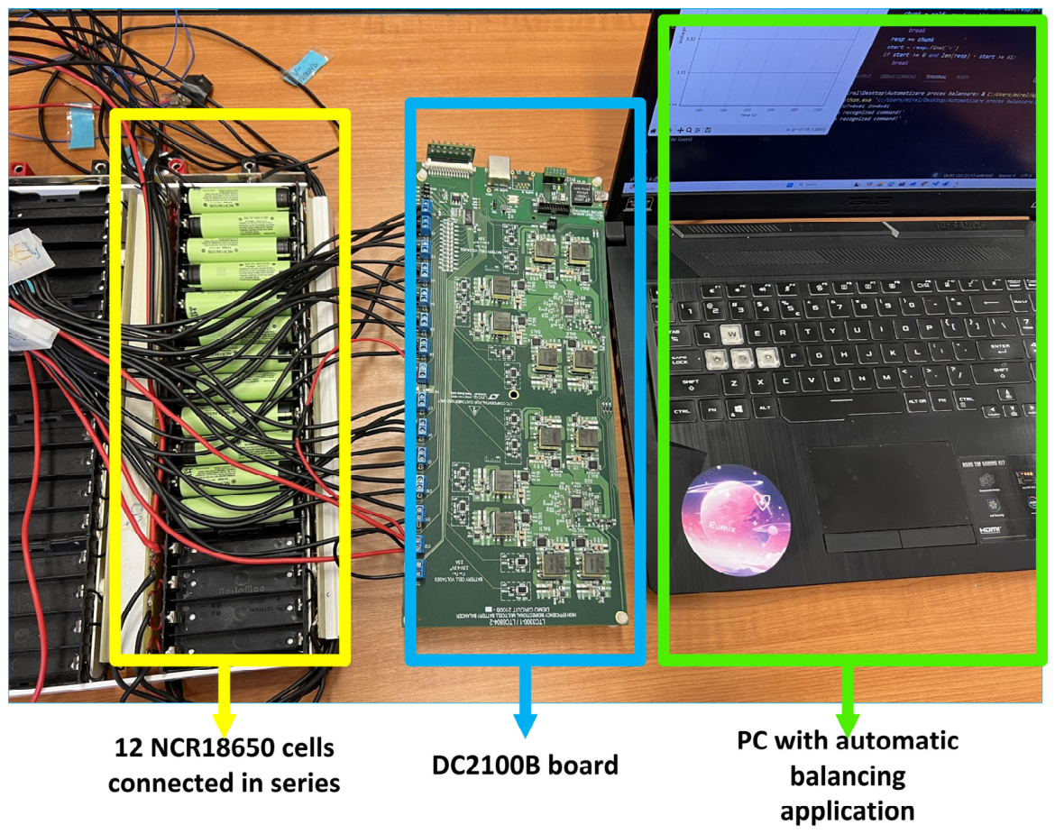
To implement predictive balancing of lithium-ion cells, the DC2100B-C balancing circuit from Analog Devices was used together with a battery pack consisting of 12 NCR18650B cells. The experimental setup is presented in Figure 26.
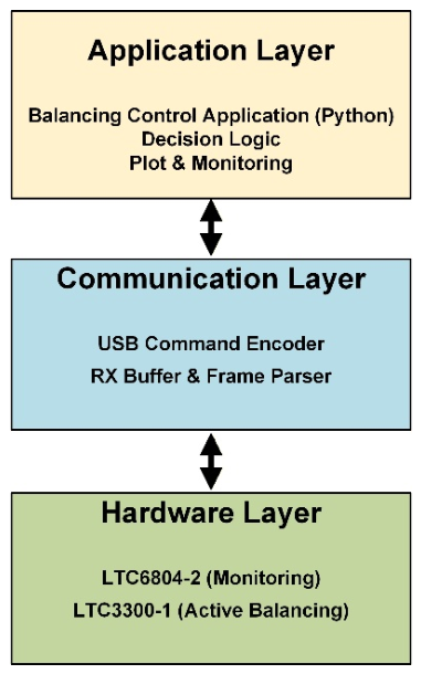
The balancing circuit provides a graphical user interface (GUI) that enables monitoring of individual cell voltages and manual selection of balancing actions (charge, discharge, or none) for each cell. However, this interface does not support automated control or the use of external algorithms. Therefore, a Python application was developed to directly interface with the DC2100B-C firmware through an ASCII-based USB communication protocol, periodically acquire cell voltages, compute balancing decisions, and send the corresponding commands to the hardware. The automatic balancing software is beyond the scope of this paper and is described in detail in a separate work currently under review. The proposed solution follows layered architecture, as shown in Figure 27.

3.2. Hardware Platform and Measurement Procedure

As presented in the previous section, the model requires three inputs: voltage, current, and temperature. The voltage is acquired from the LTC6804-2 circuit, while the current is estimated using the methodology described in Section 2.1.2. During each 3 s balancing interval, cell voltages were sampled every 10 ms while the LTC3300-1 transferred energy between cells. For each cell, a linear regression was fitted to the voltage trace V(t), and the slope dV/dt was converted into an approximate current using an empirically determined gain factor. The gain factor was selected empirically to obtain current estimates that are consistent with the observed voltage response during balancing. This method yielded a physically meaningful current estimate that reflected the actual direction and magnitude of energy movement caused by the balancing hardware. These real current values were incorporated into the temporal window used as input for the GRU model, enabling the neural network to make predictions based on both voltage dynamics and recent balancing activity.
The use of an estimated current signal based on the voltage slope introduces an inherent source of uncertainty, as it relies on the differentiation of measured voltage data. It has been shown in the literature that differentiating voltage–time signals amplifies measurement noise, which directly affects the quality of derived features and subsequent regression performance [28].
Consequently, the discrepancies observed between the estimated current and the nominal balancing current are expected and reflect the fundamental limitations of derivative-based estimation methods. In this context, the current signal used in this study should be interpreted as an approximate indicator of the system dynamics rather than an exact physical measurement.
In the absence of temperature sensors mounted on each cell, the cell temperature was approximated using the ambient temperature. This assumption is justified by the relatively low balancing currents, which are not expected to produce significant self-heating over the considered time intervals. However, this represents a limitation of the current implementation, as potential temperature gradients between cells are not explicitly captured.
To ensure a rigorous and unbiased comparison between the classical active balancing strategy and the proposed GRU-based predictive balancing, a careful cell selection and grouping procedure was performed prior to experimentation.
A large batch of new, unused Li-ion cells, all belonging to the same production lot, was initially characterized in an open-circuit condition. The purpose of this preliminary screening was to eliminate any variability originating from cell age, usage history, or manufacturing tolerances.
Based on this characterization, 24 cells were selected. These cells were then arranged into two independent 12-cell modules, designated for:
  • Module A—classical active balancing;
  • Module B—predictive GRU-based balancing.
The grouping was performed such that the voltage distributions of the two modules were statistically identical at the start of the experiment.
The 12 cells allocated to each module were chosen to ensure matching individual voltages and identical initial inter cell imbalance patterns.
This controlled pairing guarantees that both balancing strategies begin from the same initial electrochemical state, allowing for a direct, one-to-one comparison of convergence behavior and balancing efficiency after controlled balancing intervals.
By constructing two cell groups with replicated and statistically equivalent initial voltage profiles, the study isolates the influence of the balancing strategy itself, ensuring that any performance differences arise solely from the controller design rather than uncontrolled variability in the electrochemical state of the cells.
To ensure comparability, both the classical and predictive balancing procedures were executed under identical electrical, environmental, and timing conditions. Critical parameters such as quiet time before ADC acquisition, balancing ON duration, relaxation interval, and stabilization criteria were enforced uniformly across both experiments.
Voltage measurements were obtained exclusively during periods when all balancing switches were disabled to avoid transient artifacts originating from inductive energy transfer. A stabilization check based on the maximum inter-sample deviation (|dV/dt| < 1.5 mV over a 200 ms window) was required prior to accepting any final cell-voltage frame.

3.3. Balancing Algorithms and Control Logic

Both experiments followed an identical timing structure based on iterative balancing cycles. Each cycle began with the collection of sixty voltage samples per cell at a sampling frequency of 100 Hz, forming a temporal window representing the recent electrical behavior of the battery. This sampling stage was performed with all balancing switches disabled, ensuring that the data reflected the intrinsic cell behavior rather than the influence of active balancing.
Although the training dataset is sampled at 1 Hz, the experimental implementation operates at a higher acquisition rate. During each control cycle, 60 voltage samples are collected at 100 Hz with the balancing process disabled, corresponding to a short quasi-steady measurement interval.
Since the measurements are acquired under near-zero current conditions and after a relaxation phase, the resulting voltage sequence exhibits smooth temporal behavior, making it statistically consistent with the lower-frequency training data. To further reduce noise and ensure robustness, voltage measurements are filtered before being used as input to the GRU model. During active balancing intervals, voltage is sampled at 10 ms resolution for current estimation purposes. However, these high-frequency measurements are not directly used as inputs to the predictive model.
In the classical reactive balancing experiment, balancing decisions were computed using a dead-band rule: each cell voltage was compared against the pack average using a ±10 mV threshold. This value was selected based on the analysis presented for lithium-ion cells in [29], ensuring consistency with the reported electrochemical behavior. Cells lying above this threshold were discharged, cells below were charged, and all others remained off. This corresponds to a conventional rule-based balancing strategy widely used in BMS implementations.
In contrast, the predictive balancing experiment used a trained GRU model to forecast each cell voltage 5 s into the future. Instead of responding to present-state imbalance, the controller anticipated how the imbalance would evolve and applied charge/discharge decisions proactively. The same ±10 mV dead-band was applied to the predicted voltage distribution rather than the measured one. This created a direct, one-to-one comparison between classical reactive balancing and a forward-looking predictive controller.
After each balancing interval, the system entered a mandatory relaxation phase during which all balancing activity was suspended. This pause allowed the electrochemical RC dynamics of the cells to settle. The system then performed repeated filtered voltage measurements until the stabilization criterion was met. Only after stabilization was detected were the voltages logged and used for the next prediction or for classical decision-making.
Both classical and predictive controllers executed the same iterative balancing-cycle structure, with identical timing, stabilization criteria, and measurement filtering. The only difference between experiments was the decision logic: reactive (classical) versus predictive (GRU-based). This strict symmetry ensures that all observed differences in performance arise exclusively from the balancing algorithm itself, not from experimental bias or timing artifacts.

3.4. Comparison Between Conventional Balancing and Predictive Balancing

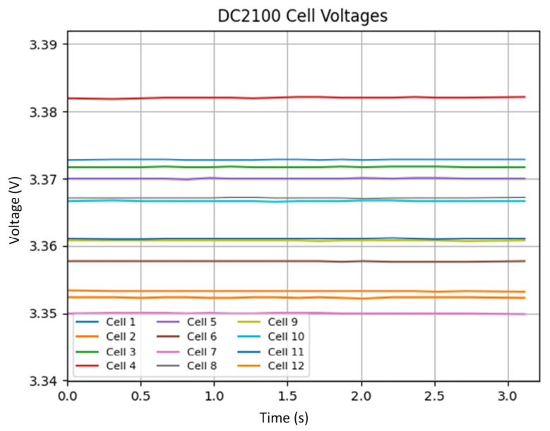
Figure 28 presents the initial voltage distribution of the two 12-cell modules, each composed of identical lithium-ion cells with nearly the same open-circuit voltage at the beginning of the experiment.
The simulations for both reactive and predictive cell balancing were carried out over a duration of 100 s to ensure that cell temperature remained approximately constant throughout the experiment. This choice is directly related to the simplification adopted in this work, namely approximating each cell’s temperature by the ambient temperature. The objective was not to fully equalize the cells, but rather to compare the behavior of reactive balancing with that of predictive balancing.
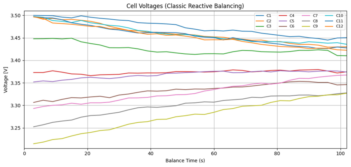
Figure 29 shows the voltage evolution of the 12 cells during classic reactive balancing. Although the convergence is slower and less uniform compared to the predictive method, the voltage difference decreases from approximately 290 mV to about 120 mV over 100 s, indicating a gradual but incomplete equalization process.
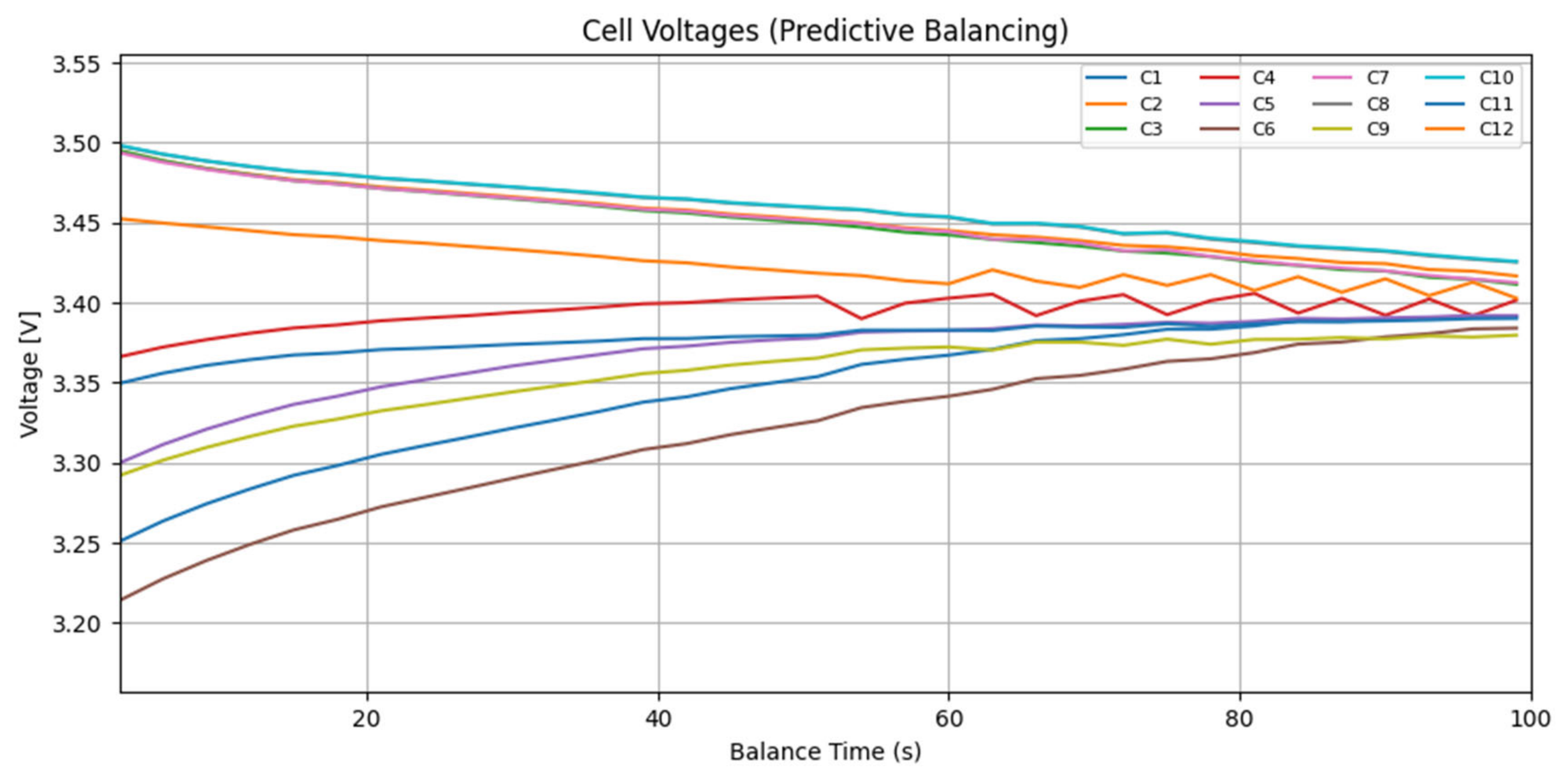
Figure 30 shows the voltage evolution of the 12 cells under predictive balancing, where the controller drives the voltages toward the average value more quickly compared to the reactive method, reducing the voltage difference from approximately 290 mV to about 50 mV within 100 s.
Over a 100 s interval, the predictive strategy required 16 command reconfigurations, compared to 25 for the classical reactive approach, indicating a reduction in switching activity and a more stable control behavior.
Table 3 presents a comparison between reactive and predictive balancing methods.
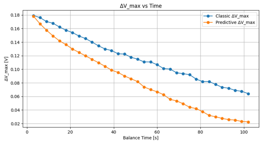
Figure 31 illustrates the evolution of the maximum cell-to-cell voltage difference (ΔV_max = max ( V i ) − min (Vi) where V i   represents the stabilized voltage of each cell measured after the relaxation phase) during 100 s of active balancing. Both balancing strategies reduce the initial imbalance of approximately 290 mV, but the predictive method achieves a substantially faster convergence. The predictive controller drives ΔV_max below 30 mV within the first 80 s and reaches a final imbalance of approximately 25 mV. In contrast, the classical reactive balancer reduces the imbalance at a noticeably slower rate and stabilizes around 65 mV after the same balancing interval. These results demonstrate that the predictive strategy is significantly more effective in equalizing cell voltages, both in terms of convergence speed and final balancing accuracy.
Figure 32 presents the final cell-voltage distribution obtained after applying both balancing strategies, highlighting the clear difference in their equalization performance. The histogram shows that the classic reactive method leaves the cells spread over a wider voltage range, indicating a less uniform final state. In contrast, the predictive balancing method produces a much tighter cluster of cell voltages around the average value, demonstrating a significantly higher degree of convergence and uniformity. This visual comparison confirms that the predictive strategy is more effective at reducing residual imbalance and achieving a compact and consistent final voltage distribution across all cells.
Figure 33 compares the final cell voltages obtained with classic and predictive balancing, showing that the predictive strategy produces a tighter and more uniform clustering of cell voltages across all 12 cells, while the classic method leaves noticeably larger differences between cells.
Table 4 summarizes the comparative performance of the reactive and predictive balancing methods in terms of voltage spread reduction and final cell voltage distribution.

4. Discussion

The results demonstrate that the predictive balancing strategy achieves faster and more uniform voltage equalization compared to the classical reactive method. While the reactive controller reduces voltage differences based solely on instantaneous measurements, the predictive approach anticipates the short-term evolution of each cell, enabling smoother and more coordinated convergence toward the average value. This behavior is consistent with the experimental results, which show a significantly lower final voltage spread and a faster reduction of ΔV_max.
These findings agree with previous studies, which indicate that data-driven and model-based control strategies generally outperform conventional reactive balancing approaches in terms of convergence speed and final accuracy.
Although the primary objective of this study was to compare reactive and predictive balancing, the trained GRU model has broader applicability within battery management systems. By capturing the temporal dynamics of cell voltages under varying operating conditions, the model can be extended to other tasks such as state-of-health estimation, early anomaly detection, voltage sag prediction under load, thermal behavior forecasting, and adaptive balancing scheduling. These directions represent promising opportunities for future research and for integration into advanced BMS architecture.

Author Contributions

Conceptualization, M.O. and D.P.; software, M.O.; validation, M.O. and D.P.; investigation, M.O.; resources, M.O. and D.P.; writing—original draft preparation, M.O.; writing—review and editing, M.O.; supervision, D.P. All authors have read and agreed to the published version of the manuscript.

Funding

This research is funded by the European Regional Development Fund (ERDF) through the Smart Growth, Digitalization and Financial Instruments Program, Contract No. 390085/11.11.2025, Project title: Ro-Green – Sustainable Electric Mobility Solutions, SMIS 336225.

Data Availability Statement

The original contributions presented in this study are included in the article. Further inquiries can be directed at the corresponding author.

Conflicts of Interest

The authors declare no conflicts of interest.

References

  1. Lester, C. Global EV Sales Reach 20.7 Million Units in 2025, Growing by 20%|Benchmark Source. Available online: https://source.benchmarkminerals.com/article/global-ev-sales-reach-20-7-million-units-in-2025-growing-by-20 (accessed on 22 January 2026).
  2. Blenkinsop, P. EU Drops 2035 Combustion Engine Ban as Global EV Shift Faces Reset|Reuters. Available online: https://www.reuters.com/business/autos-transportation/eu-relent-combustion-engines-ban-after-auto-industry-pressure-2025-12-16/?utm_source=chatgpt.com (accessed on 22 January 2026).
  3. Ranjith Kumar, R.; Bharatiraja, C.; Udhayakumar, K.; Devakirubakaran, S.; Sekar, K.S.; Mihet-Popa, L. Advances in Batteries, Battery Modeling, Battery Management System, Battery Thermal Management, SOC, SOH, and Charge/Discharge Characteristics in EV Applications. IEEE Access 2023, 11, 105761–105809. [Google Scholar] [CrossRef]
  4. Samsurizal; Afandi, A.; Faiz, M.R. Optimizing Battery Lifetime in Electric Vehicle Fast Charging Using Thunderstorm Algorithm. In Proceedings of the 2025 9th International Conference On Electrical, Electronics And Information Engineering (ICEEIE), Mataram, Indonesia, 2–3 September 2025; IEEE: Piscataway, NJ, USA, 2025; pp. 1–6. [Google Scholar] [CrossRef]
  5. Uzair, M.; Abbas, G.; Hosain, S. Characteristics of Battery Management Systems of Electric Vehicles with Consideration of the Active and Passive Cell Balancing Process. World Electr. Veh. J. 2021, 12, 120. [Google Scholar] [CrossRef]
  6. Ashraf, A.; Ali, B.; Alsunjury, M.S.A.; Goren, H.; Kilicoglu, H.; Hardan, F.; Tricoli, P. Review of Cell-Balancing Schemes for Electric Vehicle Battery Management Systems. Energies 2024, 17, 1271. [Google Scholar] [CrossRef]
  7. Shichun, Y.; Xinhua, L.; Shen, L.; Cheng, Z. Advanced Battery Management System for Electric Vehicles; Springer Nature: Singapore, 2022. [Google Scholar]
  8. Wang, Y.; Kwon, J.H.; Choi, S.C.; Zhou, G.; Park, S.J. A Modular Cell Balancing Circuit and Strategy Based on Bidirectional Flyback Converter. Batteries 2025, 11, 168. [Google Scholar] [CrossRef]
  9. Oshnoei, A.; Dk, A.A.; Safari, A.; Sorouri, H.; Blaabjerg, F. A State-of-the-Art Review on Battery Cell Balancing Strategies. Discov. Energy 2025, 5, 31. [Google Scholar] [CrossRef]
  10. Shrivastava, P.; Tey, K.S. Battery Test Data (LiFePO4 18650 Rechargeable Cell 3.3V 1100 mAh, Panasonic NCR18650B 3400 mAh, Murata VTC6 18650 3000 mAh 15A). Mendeley Data, V1. 2022. Available online: https://data.mendeley.com/datasets/29kw38kzwj/1 (accessed on 22 January 2026). [CrossRef]
  11. Ria, A.; Manfredini, G.; Gagliardi, F.; Vitelli, M.; Bruschi, P.; Piotto, M. Online High-Resolution EIS of Lithium-Ion Batteries by Means of Compact and Low Power ASIC. Batteries 2023, 9, 239. [Google Scholar] [CrossRef]
  12. Rao, V.S.; Sajja, G.S.; Manur, V.B.; Arandhakar, S.; Krishna, V.B.M. An Exploratory Study on Intelligent Active Cell Balancing of Electric Vehicle Battery Management and Performance Using Machine Learning Algorithms. Results Eng. 2025, 25, 104524. [Google Scholar] [CrossRef]
  13. Omariba, Z.B.; Zhang, L.; Sun, D. Review of Battery Cell Balancing Methodologies for Optimizing Battery Pack Performance in Electric Vehicles. IEEE Access 2019, 7, 129335–129352. [Google Scholar] [CrossRef]
  14. Mirela, O.; Pereus, D.; Simionas, A. Comparative Analysis of Active Balancing Types for Lithium-Ion Cells. In Proceedings of the 2024 IEEE 30th International Symposium for Design and Technology in Electronic Packaging (SIITME), Sibiu, Romania, 16–18 October 2024; IEEE: Piscataway, NJ, USA, 2024; pp. 352–357. [Google Scholar] [CrossRef]
  15. Babu, P.S.; Ilango, K. Comparative Analysis of Passive and Active Cell Balancing of Li Ion Batteries. In Proceedings of the 2022 3rd International Conference on Intelligent Computing, Instrumentation and Control Technologies: Computational Intelligence for Smart Systems, ICICICT, Kannur, India, 11–12 August 2022; IEEE: Piscataway, NJ, USA, 2022; pp. 711–716. [Google Scholar] [CrossRef]
  16. Abdelkareem, M.A.; Olabi, A.G.; AlMallahi, M.N.; Mahmoud, M.; Elgendi, M. A Review of Active Cell Balancing Methods in Electric Vehicles. Energy Convers. Manag. X 2025, 28, 101244. [Google Scholar] [CrossRef]
  17. Jaguemont, J.; Darwiche, A.; Bardé, F. Model Predictive Control Using an Artificial Neural Network for Fast-Charging Lithium-Ion Batteries. World Electr. Veh. J. 2025, 16, 231. [Google Scholar] [CrossRef]
  18. DC2100B-D Evaluation Board | Analog Devices. Available online: https://www.analog.com/en/resources/evaluation-hardware-and-software/evaluation-boards-kits/dc2100b-d.html (accessed on 10 December 2025).
  19. Olteanu, M.; Petreus, D.; Petri, A.M. Active Balancing Using the DC2100B-C and DC2100B-D Module. In Proceedings of the 2024 47th International Spring Seminar on Electronics Technology (ISSE), Prague, Czech Republic, 15–19 May 2024; IEEE: Piscataway, NJ, USA, 2024. [Google Scholar] [CrossRef]
  20. Camboim, M.M.; Moura, J.J.P.; Nunes, T.M.S.; De Fatima, N.C.; Rosolem, M.; Basquera, N.E.L.; Beck, R.F. A Control Strategy and Cell Balancing Speed Analysis Considering the Integrated Circuit LTC3300-1. In Proceedings of the 2022 14th Seminar on Power Electronics and Control (SEPOC), Santa Maria, Brazil, 12–15 November 2022; IEEE: Piscataway, NJ, USA, 2022. [Google Scholar] [CrossRef]
  21. LTC3300-1 Datasheet and Product Info | Analog Devices. Available online: https://www.analog.com/en/products/ltc3300-1.html (accessed on 8 January 2026).
  22. Sarbu, N.A.; Petreus, D. State of Charge Estimation of Li-Ion Batteries Using Artificial Neural Networks. In Proceedings of the International Spring Seminar on Electronics Technology, Vienna, Austria, 11–15 May 2022; IEEE: Piscataway, NJ, USA, 2022. [Google Scholar] [CrossRef]
  23. Li, X.; Ma, X.; Xiao, F.; Wang, F.; Zhang, S. Application of Gated Recurrent Unit (GRU) Neural Network for Smart Batch Production Prediction. Energies 2020, 13, 6121. [Google Scholar] [CrossRef]
  24. Lee, K.; Ko, H.; Oh, D.; Kim, J.; Oh, H. Hadamard Product Arguments and Their Applications. IEEE Access 2025, 13, 79736–79756. [Google Scholar] [CrossRef]
  25. Teixeira, R.S.D.; Calili, R.F.; Almeida, M.F.; Louzada, D.R. Recurrent Neural Networks for Estimating the State of Health of Lithium-Ion Batteries. Batteries 2024, 10, 111. [Google Scholar] [CrossRef]
  26. Huang, B.; Li, H.; Sun, J.; Sun, J.; Tian, X.; Song, K.; Zhang, S.; Wang, Z. Robust SOC Estimation for Lithium-Ion Batteries: Combination of GRU and FOMIAUKF Approach with an Improved State Transition Matrix. Energy 2025, 328, 136429. [Google Scholar] [CrossRef]
  27. Tao, S.; Jiang, B.; Wei, X.; Dai, H. A Systematic and Comparative Study of Distinct Recurrent Neural Networks for Lithium-Ion Battery State-of-Charge Estimation in Electric Vehicles. Energies 2023, 16, 2008. [Google Scholar] [CrossRef]
  28. Richardson, R.R.; Birkl, C.R.; Osborne, M.A.; Howey, D.A. Gaussian Process Regression for In-Situ Capacity Estimation of Lithium-Ion Batteries. IEEE Trans. Ind. Inform. 2017, 15, 127–138. [Google Scholar] [CrossRef]
  29. Jahn, L.; Mößle, P.; Röder, F.; Danzer, M.A. A Physically Motivated Voltage Hysteresis Model for Lithium-Ion Batteries Using a Probability Distributed Equivalent Circuit. Commun. Eng. 2024, 3, 74. [Google Scholar] [CrossRef]
Figure 1. Vehicle C O 2   emissions levels.
Electronics 15 01985 g001
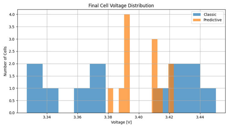
Figure 2. Battery Management System—block diagram.
Electronics 15 01985 g002
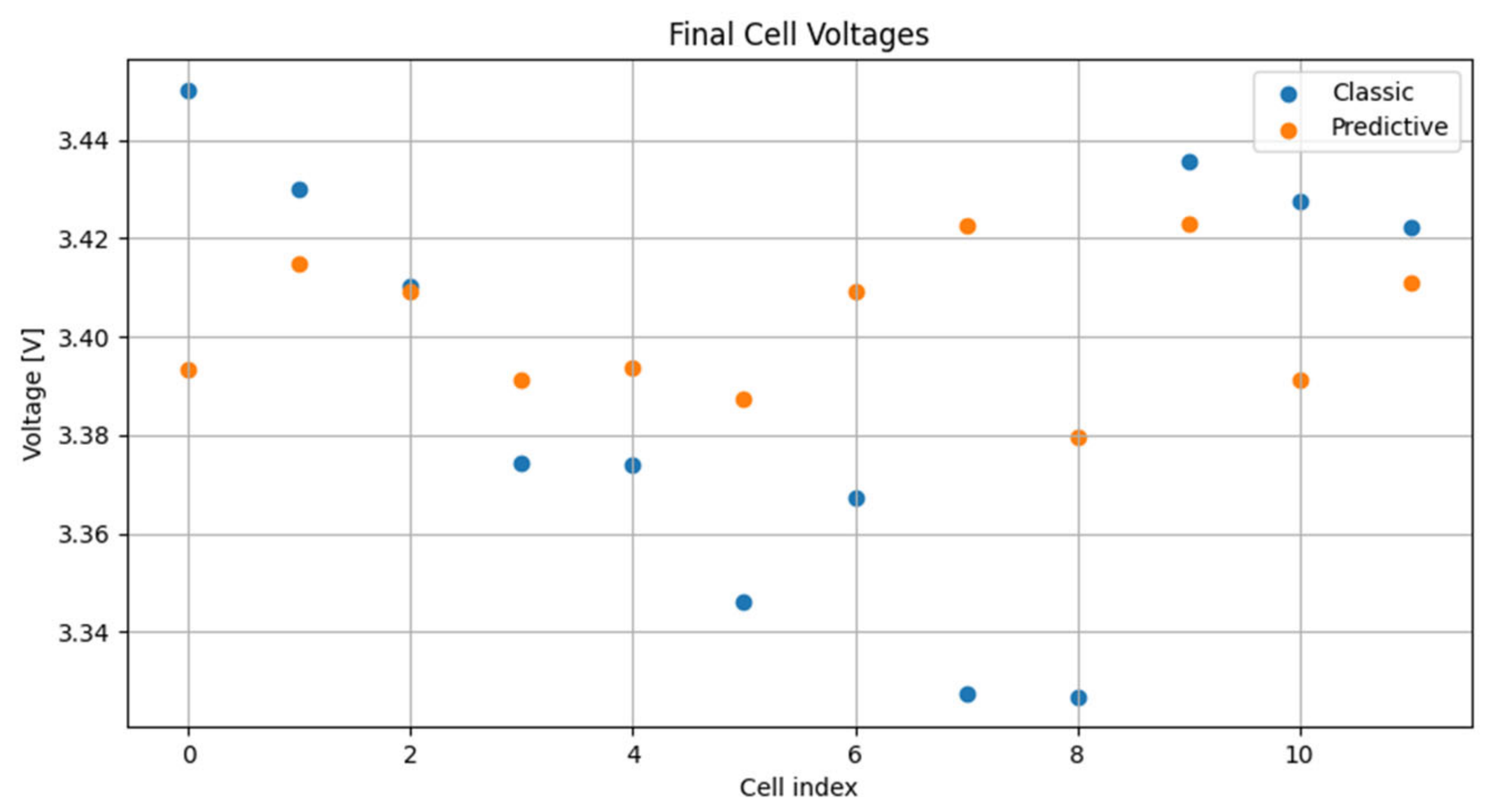
Figure 3. Passive balancing vs. Active Balancing.
Electronics 15 01985 g003
Figure 4. A chart of the basic cell-balancing topologies.
Electronics 15 01985 g004
Figure 5. Active cell balancing using capacitors (a) Single Switched Capacitor topology; (b) Switched Capacitor topology; (c) Double-Tiered Switched Capacitor topology; (d) Modular Switched Capacitor topology [14].
Electronics 15 01985 g005
Figure 6. Active cell balancing using inductors (a) Single Inductor Topology; (b) Multi-Tiered Inductor Topology [7].
Electronics 15 01985 g006
Figure 7. Converter-based active balancing topologies: (a) Buck converter balancing; (b) Boost converter balancing; (c) Buck-boost converter balancing; (d) Cuk converter balancing [7].
Electronics 15 01985 g007
Figure 8. Battery Management System with LTC3300-1/LTC6804-1.
Electronics 15 01985 g008
Figure 9. The configuration of the analyzed modular cell balancing circuit with bidirectional flyback converter.
Electronics 15 01985 g009
Figure 10. The topology of the synchronous flyback converter in the cell balancing circuit.
Electronics 15 01985 g010
Figure 11. Primary and Secondary Currents During Discharge of Cell 1.
Electronics 15 01985 g011aElectronics 15 01985 g011b
Figure 12. Primary and Secondary Currents During Charge of Cell 1.
Electronics 15 01985 g012aElectronics 15 01985 g012b
Figure 13. Current profiles: (a) DST; (b) FUDS; (c) UDDS; (d) US06; (e) WLTS; (f) HPPC.
Electronics 15 01985 g013
Figure 14. Architecture of artificial neurons.
Electronics 15 01985 g014
Figure 15. Architecture of a recurrent Neural Network.
Electronics 15 01985 g015
Figure 16. Comparison of: (a) RNN; (b) LSTM; (c) GRU.
Electronics 15 01985 g016
Figure 17. Activation function: (a) sigmoid; (b) tanh.
Electronics 15 01985 g017
Figure 18. Architecture of the proposed GRU-based voltage prediction model.
Electronics 15 01985 g018
Figure 19. Computation flow within the GRU unit [26].
Electronics 15 01985 g019
Figure 20. Performance of the GRU-based voltage prediction model: (a) comparison between measured and predicted voltage at t + 1; (b) distribution of prediction error.
Electronics 15 01985 g020
Figure 21. Prediction performance: (a) predicted vs. measured voltage; (b) prediction error at t + 1.
Electronics 15 01985 g021
Figure 22. Performance of the GRU-based voltage prediction model: (a) comparison between measured and predicted voltage at t + 5; (b) distribution of prediction error.
Electronics 15 01985 g022
Figure 23. Prediction performance: (a) predicted vs. measured voltage; (b) prediction error at t + 5.
Electronics 15 01985 g023
Figure 24. Performance of the GRU-based voltage prediction model: (a) comparison between measured and predicted voltage at t + 10; (b) distribution of prediction error.
Electronics 15 01985 g024
Figure 25. Prediction performance: (a) predicted vs. measured voltage; (b) prediction error at t + 5.
Electronics 15 01985 g025
Figure 26. Experimental setup for the active cell balancing system, including the battery pack, DC2100B board, and control PC.
Electronics 15 01985 g026
Figure 27. Software Architecture Overview.
Electronics 15 01985 g027
Figure 28. Initial voltage distribution.
Electronics 15 01985 g028
Figure 29. Reactive balancing process.
Electronics 15 01985 g029
Figure 30. Predictive balancing process.
Electronics 15 01985 g030
Figure 31. Maximum cell-to-cell voltage deviation.
Electronics 15 01985 g031
Figure 32. Final cell-voltage distribution for each cell.
Electronics 15 01985 g032
Figure 33. Final cell-voltage distribution.
Electronics 15 01985 g033
Table 1. Summary of the experimental dataset.
Temperature (°C)Profiles UseTotal Samples
−5 °C
5 °C
25 °C
45 °C
1.5 C2058
1 C3310
0.5 C7074
DST24,487
FUDS19,323
UDDS24,262
HPPC60,000
WLTS24,280
US0615,781
Total Dataset Samples 722,300
Table 2. Prediction error metrics for different horizons.
HorizonMAE [mV]RMSE [mV]
t + 11426.5
t + 537.158.9
t + 1043.161.1
Table 3. Comparison between reactive and predictive balancing methods.
MetricReactive BalancingPredictive Balancing
Initial voltage difference290 mV290 mV
Final voltage difference 120 mV50 mV
Convergence time100 s100 s
Convergence behaviorSlowFast
Command reconfigurations2516
Control strategyReactivePredictive (GRU-based)
Table 4. Comparative performance based on ΔV evolution and final voltage distribution.
MetricReactive BalancingPredictive Balancing
ΔV_max reduction64%88%
Final voltage dispersionWide spreadNarrow spread
Disclaimer/Publisher’s Note: The statements, opinions and data contained in all publications are solely those of the individual author(s) and contributor(s) and not of MDPI and/or the editor(s). MDPI and/or the editor(s) disclaim responsibility for any injury to people or property resulting from any ideas, methods, instructions or products referred to in the content.